A Dynamic and Incentive Policy for Selecting Device-to-Device (D2D) Mobile Relays
Abstract
User-to-network relaying enabled via Device-to-Device (D2D) communications is a promising technique for improving the performance of cellular networks. Since in practice relays are in mobility, a dynamic relay selection scheme is unavoidable. In this paper, we propose a dynamic relay selection policy that maximizes the performance of cellular networks (e.g. throughput, reliability, coverage) under cost constraints (e.g. transmission power, power budget). We represent the relays’ dynamics as a Markov Decision Process (MDP) and assume that only the locations of the selected relays are observable. Therefore, the dynamic relay selection process is modeled as a Constrained Partially Observable Markov Decision Process (CPOMDP). Since the exact solution of such framework is intractable to find, we develop a point-based value iteration solution and evaluate its performance. In addition, we prove the submodularity property of both the reward and cost value functions and deduce a greedy solution which is scalable with the number of discovered relays. For the muti-user scenario, a distributed approach is introduced in order to reduce the complexity and the overhead of the proposed solution. We illustrate the numerical results of the scenario where throughput is maximized under energy constraint and evaluate the gain that the proposed relay selection policy achieves compared to a traditional cellular network.
Index Terms:
Device-to-Device (D2D) communications, relay selection, mobility, Constrained Partially Observable Markov Decision Process (CPOMDP)I Introduction
In D2D enabled cellular networks, user to network relaying can be handled for improving the performance of cellular networks. Under realistic assumption that relays are in mobility, it is crucial to define a strategy for designating the relays that will respectively serve each Master User Equipment (MU) in the network. In this paper, we propose a relay selection policy that maximizes the performance of cellular networks (e.g. throughput, reliability, coverage) under cost constraints (e.g. transmission power, power budget). We assume that the relays’ dynamics are represented by a Markov Decision Process (MDP) where the Master User Equipment (MU) cannot directly observe the locations of all the potential relays that have been discovered. Therefore, the sequential relay decision process is modeled by a Constrained Partially Observable Markov Decision Process (CPOMDP). Since the exact solutions of such framework are computationally intractable to find, we have developed an approximated solution as well as discussed the existing trade-off between its complexity and its preciseness. Moreover, proving the submodularity property of the reward and cost functions leads us to propose a greedy form of the approximated solution. Numerical results are presented to endorse our relay selection policies and to show how introducing D2D relaying can highly improve the performance of cellular networks. Furthermore, a system-level simulator is developed in order to implement our strategy of relay selection and to test its performance in a nearly realistic cellular network.
II Concept and related work
In traditional cellular networks, single hop communications are deployed between the users and the Base Station (BS). However, introducing relays to cellular networks has become one of the major concern of cellular network planners that aim to improve the capacity and the coverage of their networks. The emergence of D2D communications encourages the deployment of User Equipment (UE)-to-Network relaying functionality. D2D communications will take place between the MU and the relays however cellular communications are maintained between the relays and the BS. The main advantages of such relaying feature is: (i) improving the performance of the network (e.g. capacity enhancement, coverage extension, transmission power reduction, load balancing, network offloading etc.) and enabling new services (e.g. data on demand).
D2D relaying technique has been the subject of interest of significant research in both academia and industry. Several tools have been used for evaluating the performance of this technique. Stochastic geometry is used for analytically modeling and analyzing the performance of cellular network with fix D2D relays in [1] and mobile D2D relays in [2]. Monte-Carlo simulations in [3] and [4] show how enabling D2D communications to carry relayed traffic can enhance the capacity and coverage of cellular networks. A system-level simulator in [5] was developed to evaluate the extension of the cellular coverage due to D2D relaying.
Despite the performance gain that UE-to-Network relaying has promised, several challenging issues require further investigation. One can ask how the relays should be strategically positioned in order to optimize the performance of the network.Sharing the spectrum between D2D and cellular communciations is one of the existing challenges. Using stochastic geometry modeling, authors in [6] studied underlay D2D enabled cellular networks. They analytically derived the tradeoff generated by the spectrum partition between D2D and cellular communications and they deduce the optimal spectrum partition that guarantees the fairness in the network. Several solutions of power and/or resource allocation in D2D relayed cellular networks have been studied in the recent literature. The work [7], that proposes a distributed resource allocation for D2D relay-aided cellular networks using game theory tool, exposes a summary of the different existing centralized and distributed resource allocation schemes. In addition to resource and power allocation, a mode and path selection algorithm was developed and simulated in [8]. Furthermore, Constrained Markov Decision Process (CMDP) problems were formulated in [9] and [10] to obtain the optimal decision of packet scheduling that mobile relays should take.
One of the main challenges of D2D relay-aided cellular networks is to decide how relays should be selected in order to achieve the performance of cooperative relaying. Due to relay mobility, a dynamic relay selection policy is unavoidable. Indeed, a relay selected at one position can be no longer helpful at another position. In this work, we address this question by proposing a dynamic relay selection strategy that MU may take for optimizing a certain performance metric (e.g. throughput, coverage, reliability etc.). Since the relaying functionality is costly for the relays (e.g. in terms of energy, data consumption etc), we propose to charge MU s for using their selected relays. This cost aims to encourage the users to behave as potential relays. Based on the fact that the reward as well as the cost of each relay depends on its location, we propose a dynamic relay selection policy that maximizes some Quality of Service (QoS) metric of cellular networks while satisfying some cost constraints.
II-A Related Work
Relay selection is crucial for improving the performance of D2D relay-aided cellular networks. The rich literature on relay selection problems can be divided into two categories: mobile relay selection and fix relay selection schemes. Most of the previous works considers fix relay selection scenarios. Some of these schemes are briefly presented in the following. Based on a stochastic formulation, authors in [11] propose a fully distributed single relay association scheme that aims to increase the spectral efficiency of the network. An energy efficient relay selection was proposed in [12] based on a Discrete Time Markov Chain (DTMC) modeling of the relay node with Discontinuous Reception (DRX) mechanism. Based on an iterative technique, [13] proposes a joint relay selection and power allocation problem scheme for relay-aided D2D underlying cellular networks. The work in [14] uses a queuing theory model to propose a single relay selection scheme that optimizes the network in terms of relay remaining battery life, end-to-end data rate and end-to-end delay criteria. For underlay D2D enabled cellular networks, interference is mitigated between cellular and D2D communications by considering a distributed relay selection algorithm in [15].
However, the aforementioned works do not take user mobility into account but consider fix relays which limits their applicability in cellular mobile networks. Considering the mobility of the relays seems to be a challenging scenario. Mobile relays have been the subject of the work in [16]. Based on the knowledge of the relay mobility pattern, a dynamic relay selection scheme aiming to minimize the cost of relaying under QoS requirements was proposed. The studied optimization model is based on CMDP. Since relay selection appears as decision making process, several Markov Decision Process (MDP) based formulation has been studied in order to propose optimal relay selection scheme. For example, while predicting the channel states of the available relays, authors in [17] address a relay selection policy that maximizes the long term transmission rate. This decision strategy is obtained by solving a Partially Observable Markov Decision Process (POMDP) with dynamic programming-based algorithm.
II-B Contribution and Organization
The use cases of D2D communications that will be studied in this paper is user to network relaying in cellular networks. The mobility of the relays is the main challenge for relay selection decision. We propose a dynamic relay selection policy that maximizes a certain performance metric of the network (e.g. throughput, reliability, coverage etc.) under cost constraints (e.g. energy consumption, data consumption etc.). The main contribution in this work can be summarized as follows:
- •
Constrained Partially Observable Markov Decision Process (CPOMDP) formulation of the sequential relay selection process that a MU will decide and discussion concerning the complexity of this problem.
- •
Proposition of a dynamic policy of relay selection that approximately optimizes the formulated problem based on a greedy point based value iteration.
- •
Extending the results to multiple users scenario.
- •
Numerical results as well as system-level simulations show the performance that cellular networks may gain by implementing the proposed relay selection policy.
The main particularity of this work compared to other relay selection schemes previously proposed in the literature is the following:
- •
The consideration of a realistic scenario where relays are in mobility, thus dynamic relay selection scheme is necessary.
- •
The cellular network performance is optimized under cost constraints.
- •
The sequential relay decision process is modeled by a Constrained Partially Observable Markov Decision Process (CPOMDP) (and not a CMDP) since the states of the potential relays cannot be observed until these relays are selected by the MU.
- •
An approximated solution is proposed for avoiding the intractability of exact solutions. A trade-off between the preciseness of the approximated solution and its complexity is derived.
- •
The relay selection is not limited to one relay, thus the performance gain is improved due to the increasing in the cooperative diversity order. Actually, the proposed relay selection policy aims to maximize the performance of the network under cost constraints without any constraints on the number of chosen relays.
- •
The relays’ mobility pattern is assumed communicated to the agent decision maker ( MU or the BS).
The rest of this paper is organized as follows. Section III describes the system model for a single MU scenario. Section IV formulates the optimization problem as a CPOMDP. Since the exact solutions of such problem are intractable to find, a low-complexity dynamic relay selection, called Constrained Point-Based Value Iteration (CPBVI), is proposed in section V. The submodularity property is verified for this problem, thus a greedy form of this approximation, called Greedy Constrained Point-Based Value Iteration (GCPBVI), is deduced. These results are extended to a multi-MU scenario in section VI. For this scenario, a distributed approach is exposed for reducing the complexity of centralized solutions. Numerical results in section VII corroborate our claims. The performance enhancement of the cellular networks is shown in section VIII by implementing the proposed relay selection scheme in a system-level simulator. Section IX concludes the paper whereas the proofs are provided in the appendices.
III System Model
For the sake of clarity, we describe the system model for a single MU scenario. We show that extending the result to multi-MU scenario is a straight forward process.
III-A Network model
We consider a single cell scenario with one MU and a set of potential mobile relay. MU is allowed to use D2D communications to access the network via mobile relays and by that improving the performance of its cellular communications. As figure 1 shows, the MU is allowed to use D2D communications to access the network via mobile relays. MU discovers nearby potential relays by launching a discovery process of period . The time between two discovery processes is partitioned into decision epochs (e.g. Time Transmission Interval (TTI) in Long Term Evolution (LTE) networks) of constant duration (with ). The goal of this work is to determine the relay selection policy that should be applied by the MU at each epoch in order to maximize its cumulative reward under cost constraints.
denotes the set of existing potential relays (from index to ) as well as the direct cellular link (index ). The relay selection policy consists in deciding whether the MU will have direct communication with the network or will pass by some mobile relays. In the latter case, this policy chooses the subset of relays that will be used for attaining the network. Please note that D2D relaying can be applied to both Downlink (DL) and Uplink (UL) communications. Due to the practical consideration that mobile terminals do not support simultaneous signal transmission and reception, a two-phases transmission scheme is assumed. Therefore, for UL (resp. DL) relayed communication, the transmission protocol is divided into two phases: (i) in the first phase the relay receives the data from the MU (resp. BS) and (ii) in the second phase the relay transmits the received data to the BS (resp. MU).

III-B Mobility Model
Relays’ locations in a service coverage area are quantized and represented by a set of regions . We assume that the relays remain in the same region during a decision epoch. We denote by the location of relay at epoch . In the next epoch, the location of each relay is changed (i.e. by either staying in the same region or moving to another neighboring region). Thus, the mobility of relay is modeled by a transition matrix where each element of this matrix denotes the probability that relay moves from region to region in the next decision epoch. In this work, we assume that the MU is aware of the mobility pattern of each discovered relay (i.e. equivalent to the relay’s transition matrix). The vector denotes the location of the potential relays at epoch .
We underline that the location of each relay is changing over time epochs based on its transition probability matrix and independently from the fact that this relay has been or not selected. We assume that the MU will be able to know the current localization region of only the chosen relays. On the other hand, the MU will just have a certain belief of the locations of the non selected relays. It is a practical assumption because when a relay is selected by the MU some signaling is exchanged between these two equipments in order to allow D2D communications. This exchange may include some information that indicates the region of the selected relay. However, when the relay is not selected then no need for any signaling between the MU and the relay since no communication will take place between these two equipments. In this case, recognizing the region of the relays requires an overhead of signaling which can be avoided.
III-C Cost and Reward Model
We propose a relay selection policy that aims to optimize a cellular reward under cost constraints. Here, cost and reward models are described. The reward function, which depends on the relay’s location, represents the benefit of choosing a relay in terms of throughput and/or reliability and/or coverage etc. The cost function, which depends on the relay’s location, defines the charge that the MU owes to each selected relay (i.e. in terms of energy and/or incentive budget etc.). We respectively denote by and the reward and the cost of the relay in location . We assume that when the MU chooses a set of relays then the total reward (resp. cost) is the sum of the reward (resp. cost) of each relay in the chosen set. We denote by the vector such that if relay is selected and otherwise. Thus, the total reward and cost at a given state are given by:
| (1) |
| (2) |
IV Problem formulation
Enabling user to network relaying functionality based on D2D communications leads to the following question: which mobile relays should be chosen by the MU for ensuring an enhancement in cellular communications. This decision depends essentially on the reward and cost parameters of the discovered relays. The main challenge of such relay selection policy remains in the mobility of these potential relays. The goal is to make the relay selection decision () that optimize the following:
| (3) |
where is a discount factor that represents the difference in importance between future rewards (resp. costs) and present rewards (resp. costs).
The considered reward model includes a large scope of reward metrics. In the following we give few examples that indicate how the reward mode 1 can be applied:
- •
Throughput criteria: different packets are transmitted to the selected relays, thus the total throughput is the sum of the throughput of each selected link. Considering the example of Shannon capacity over a bandwidth W, the total reward is given by
- •
Reliability criteria: same packets are transmitted to the selected relays, thus the error probability is equal to the product of the error probability of each selected link . For example, in the case of considering the bit error ratio in the case of Quadrature Phase-Shift Keying (QPSK) modulation and Additive White Gaussian Noise (AWGN) channel, the error probability of relay at state can be written as follows:
When action is taken, then . Thus, minimizing this error probability corresponds to maximizing the of the probability error of each selected link
Therefore, we can express the reliability reward as of the error probability in order to have the overall reward as the sum of the reward of each selected relay
The process above can be applied to any other error probability function (e.g. [18]).
- •
Coverage probability criteria: same packets are transmitted to the selected relays, thus the overall outage probability is equal to the product of the outage probability of each selected link. Similarly to reliability criteria, we can express the coverage reward as of the outage probability in order to have the overall reward as the sum of the reward of each selected relay.
The considered cost model can be applied to a wide range of cost metrics. In the following, we give some examples to illustrate how the cost model given by 2 can be applied:
- •
Energy criteria: the total consumed energy is the sum of the energy consumed by each selected relay. For example, if we denote by the transmission power of relay when it is in state , thus:
- •
Incentive criteria: the total charged cost is equal to the sum of the incentive budget required by each selected relay. For example, one can denote by the tokens used by relay in state , thus:
IV-A Restless Markov Multi-armed Bandit (RMAB) representation
The MU relay selection procedure consists of choosing a limited set of mobile relays that optimizes its subjective function under cost constraints. However, the positions of the potential relays are partially known at the epoch of decision and turn to be more observable as time passes. This problem can be modeled by a RMAB due to the three following reasons:
- •
It is a multi-armed bandit problem because the set of potential relays represents the arms among which the MU will make its selection.
- •
It is a Markov multi-armed bandit problem because the location of the arm is modeled by a discrete, irreducible and aperiodic Markov chain with finite space and transition probability matrix (i.e. relays’ locations are the states of this RMAB)
- •
It is restless because the potential relays change their location/state from a decision epoch to another independently from the current decision (whether they’ve been selected or not).
The objective of the relay selection strategy is to optimize problem 3 through a sequence of selection . For each selection decision, there exists a trade-off between exploitation phase that tends to achieve the highest expected reward and exploration phase that tends to get more information concerning the positions of other relays. In the sequel, we describe the CPOMDP formulation equivalent to the proposed RMAB problem.
IV-B CPOMDP formulation
In order to study the RMAB defined above, we formulate its equivalent finite-horizon CPOMDP which is characterized by the tuple defined below:
- •
State denotes the state vector or the location vector of the potential relays (where for all ). represents the set of all possible state vectors with .
- •
Action denotes the vector of the binary actions such that specifies whether relay is selected () or not () for all . represents the set of the indexes of the selected relays. denotes the set of all action vectors, it contains elements.
- •
Transition function represents the probability of transiting between states. characterizes the probability of passing to state in the next decision epoch knowing that the current state is . Assuming that the relays’ mobility are independent and described by their transition probability matrix, then . This probability is independent from the action since the selection decision has a purely observational role (i.e. the relays change their locations independently from the fact that they have been selected or not). represents the transition matrix of elements.
- •
Observation denotes the observation vector of the potential relays. Selecting a relays leads to the observation of its state, hence when relay is not selected then otherwise . The set of all observations is denoted by .
- •
Conditional observation probability represents the probability of receiving an observation knowing that the decision policy takes action and by that transits to state , we define:
- •
Reward is the reward achieved by taking action when the potential relays are in state . We suppose for all and .
- •
Cost is the cost charged by taking action when the potential relays are in state . We suppose for all and .
- •
Initial belief is a vector of elements that denotes the initial distribution probability of being at each state .
- •
Horizon of the CPOMDP represents the number of epochs of the relay selection policy between two successive discovery processes (i.e. is the discovery periodicity).
- •
the cost threshold.
- •
as a discount factor.
The MU chooses its action as function of the history of observations and actions that have been executed in the past. The result of [19] demonstrates that using the belief states for defining the optimal policy provides as much information as using the entire history of actions taken and observations received. Indeed, there is no need to explicitly save this history but having the current belief state is sufficient for deciding the upcoming actions.
Therefore, a POMDP can be represented as a belief MDP where every belief is a state. Since there is infinite belief states, this MDP is defined over a continuous set of belief states. At a given epoch , the MU gathers all the information concerning the past decisions in the belief state defined as follows:
| (4) |
The belief vector of elements is denoted by . By analogy, we define as the belief state of the mobile relay and its corresponding belief vector:
Given the fact that the mobile relays move independently, the belief state , at a given state and epoch , can be deduced from the belief state of each relay as follows:
The belief state of relay at epoch is recursively computed based on the previous belief state , previous action and current observation
| (5) |
where . Therefore, when the action (with equivalent set ) is taken and the observation is detected then the belief of being in state is updated as follows:
| (6) |
The belief states pursue a Markov Process where the belief state at a given epoch depends on the belief, action and observation of the previous epoch with the following transition function:
| (7) |
| (8) |
A policy is a function that determines the action to take at each belief state . For a given initial policy , a policy is characterized by a value function for the reward evaluation and for the cost evaluation:
| (9) |
| (10) |
where the belief-based reward and the belief-based cost are:
| (11) |
| (12) |
The value functions and at epoch and under policy are given by the Bellman equation:
| (13) |
| (14) |
where is given by equation (8).
The action-value function is the reward of taking action at epoch and following policy thereafter:
| (15) |
The action-value function is the cost of taking action at epoch and following policy thereafter:
| (16) |
The objective of the optimal relay selection policy is to achieve the highest reward under cost constraints. The optimal policy maximizes the value function under constraints on . There exists an optimal Markov policy which defines the action to be executed for each belief state supposing that the upcoming actions will be chosen in an optimal manner. The value of the optimal policy function satisfies the Bellman optimal equation:
| (17) |
s.t.
We define the Bellman dynamic operator:
V Relay Selection Policies
V-A Exact Solution of CPOMDP
[19] shows that the value function of POMDP is a Piecewise-Linear Convex (PWLC) function over the infinite belief simplex (denoted by ). Thus, the value function can be characterized by a finite set of value function vectors (hyperplans) [20]. Each vector represents the optimal value of the value function in a given region of the belief space. The exact solution of the CPOMDP, proposed in [21], is inspired from the value iteration of POMDP. This technique presents the value functions and as PWLC functions over the infinite belief simplex . Therefore, the reward and cost value functions and are represented as a finite set of -vectors pairs .
Considering the set of -vectors pairs at epoch , then the set at the following epoch is constructed by applying the following dynamic programming operator over all the action-observation pairs: 11 1 The cross sum operator of two sets and is given by the set : .
|
|
Thus,
This dynamic programming update produces :
At the worst case, each dynamic programming update will generate an exponentially increasing pairs of -vectors. However, some pairs of -vectors are never the optimal one in any region of the belief simplex (i.e. called useless vectors). Therefore, for mitigating this exponential explosion, different pruning algorithms were developed in order to exclude these useless vectors. For POMDP problem, [20] have proposed an algorithm that identifies these useless vectors in order to ignore them. For CPOMDP a pruning operation for the value functions were proposed in [21] in order to generate the minimal set of pairs of -vectors at each iteration. The pruning function that we adopt for implementing this solution consists of keeping each pair that satisfies the cumulative cost constraint and that have the higher cumulative reward in some region of the belief simplex . This can be decided by solving a Mixed-Integer Linear Program (MILP) for each pair of -vector (one can refer to equation (3) in [22]). This pruning method eliminates each pair of vectors that violates the cumulative cost constraint at a given iteration . Note that this operation may lead to a suboptimal policy. Therefore, randomized policies are the subject of further study to achieve the optimal solution of CPOMDP.
As presented in algorithm 1, the iteration of the exact solution of CPOMDP follows this procedure: (i) exact dynamic programming to generate the pairs -vectors, (ii) pruning operation, based on a mixed integer linear program, that produces the minimal set of -vectors, (iii) deducing the optimal value function.
Due to PWLC propriety of the value function, the value iteration algorithm of CPOMDP is limited to find the set of -vector pairs that represents the value functions and given the previous set . Constructing the set of hyperplans by considering all the possible pairs of observations and actions over the previous set has an exponential complexity of (i.e. considering the states it gives ). Since many pairs of vectors in are dominated by others, pruning algorithms are developed in order to eliminate useless vectors and find the smallest subset sufficient for representing the value functions. Given the exponential complexity increase at each iteration, the necessity of pruning operations is obvious. However, pruning techniques consists on resolving a Mixed-Integer Linear Program MILP for each pair of -vector. Therefore, value iteration algorithm for CPOMDP remains computationally demanding to solve as the size of the problem increases. This requires the exploration of approximated solutions for finding the optimal solution of CPOMDP.
V-B CPBVI
Since the value iteration algorithms for POMDP do not scale to highly sized real problems, an approximate POMDP planning solution called Point-Based Value Iteration (PBVI) was introduced in [23]. Most POMDP problems unlikely reach most of the points in the belief simplex . Thus, it is preferable to focus the planning on the most probable belief points without considering all the possible belief points as exact algorithms do. Instead of considering the entire belief simplex, PBVI limits the value update to a representative small set of belief points . An -vector is initialized for each belief point and then the value of this vector is iteratively updated. The PBVI algorithm can be simply adapted to solve CPOMDP problem (e.g. [22]).
V-B1 CPBVI algorithm
We call CPBVI the proposed suboptimal algorithm of relay selection inspired from PBVI. Algorithm 1 is modified in such a way that the value function update is restrictively done over a finite belief set and then the pruning algorithm chooses the dominated pair of vectors for each belief state . This allows the CPBVI algorithm to achieve much better scalability. At each iteration, CPBVI follows the following steps for computing the set of vectors at epoch given the previous one :
- 1.
The first step is to generate the sets and for all , all and all pairs of -vectors :
- 2.
The next step is to generate the sets and for all :
Contrarily to PBVI algorithm used for approximately solving POMDP, we need the cross-summation overall the possible observations to find the sets and . This cross-summation is mandatory in order to not impose the cost constraint on each action and observation pair while computing the best pair of -vector for each belief state . A local combinatorial explosion of is required.
- 3.
The final step is the pruning operation. In our algorithm we propose to find one optimal pair of -vectors for each belief point as follows:
Note that the proposed deterministic policy ensures the satisfaction of the cumulative cost constraint 3 at each epoch. Thus, such deterministic policies can be sub-optimal for CPOMDP (by analogy to CMDP). Ideally, randomized policies that consider convex combination of -vectors during the pruning operation can be applied to guarantee optimality.
- 4.
Finally .
In order to study the complexity of each iteration of the CPBVI algorithm, we detail the complexity of each step. Step 1 creates pair of vectors because the previous set of -vector is limited to components. The cross sum in the second step generates operations. Since the size of the -vector set remains constant (equals to ), each CPBVI update takes only polynomial time to be executed. This complexity is linear with the number of possible actions . However, in our settings, leads to a poor scalability of our algorithm in the number of potential relays . Therefore, we propose, in subsection V-C, a greedy version of the CPBVI algorithm.
V-B2 Performance Evaluation
A belief set is characterized by a density which is the maximum distance from any point in the belief simplex to the set .
Definition V.1.
The density of a belief set is defined as:
| (18) |
We denote by and the reward and cost value functions produced by the proposed CPBVI algorithm. From theorem 1 of [23], we know that for a belief set of density , the errors and of the CPBVI algorithm at horizon are bounded as follows:
| (19) |
One can remark that this result does not take into account the case where the discount factor is equal to . Hence, we extend the result to the case where .
Theorem V.2.
At horizon and discount factor , the errors and of applying the CPBVI algorithm over a belief set of density are bounded as follows:
| (20) |
V-B3 Belief set Selection
The bound calculation of the error that occurs with the application of the CPBVI algorithm shows the importance of the selected belief set . Indeed, these bounds are proportional to the density of the chosen belief set . For this reason we show how to find the belief set, denoted by , that limits the upper bounds and to a small . It is obvious that a trade-off exists between the size of the belief set and the precision of the value functions .
We denote by the set of reachable belief states in our settings with an horizon . Therefore, for a relay , the corresponding set of reachable beliefs is given by:
| (21) |
where correspond to the transition matrix to the power of (i.e. the transition matrix from a state to another after epochs). Therefore, the set contains vectors of elements. Thus, considering all the candidate relays , the size of the overall reachable belief points for an horizon is given by .
It is clear that, for an horizon , considering the set of reachable belief points as the belief set of the CPBVI algorithm minimizes the errors and (i.e. because all the reachable belief points were taken into account in ). However, due to the exponentially large size of the set , we propose to construct a smaller set of belief points that is sufficient for upper bounding the performance errors and by a small . We denote by the set of reachable states after passing epochs and knowing that the initial state is (i.e. represents the neighbor states of ). For constructing the belief set , we give the following definition.
Definition V.3.
We define the -belief set for an initial state and an horizon as follows:
| (22) |
with the transition matrix power to .
We emphasize that the size of a set is bounded by .
Theorem V.4.
The density of an -belief set is bounded by:
| (23) |
where is the highest eigenvalue of the transition matrix of relay and with the stationary distribution corresponding to .
Proof.
Please refer to the proofs section A. ∎
Theorem V.5.
For an initial state and a problem of horizon and discount factor , the belief set that should be selected in order to achieve an performance (i.e. and ) is given by:
| (24) |
with
Proof.
Please refer to the section B for the proof of the theorem as well as its extension to . ∎
V-C Greedy CPBVI
The computational complexity of each iteration of the CPBVI algorithm is proportional to the size of the set of actions which increases exponentially with the number of potential relays . Therefore, we propose a GCPBVI algorithm that exploits greedy maximization which consists of iteratively choosing the relays that should be selected in the aim of optimizing the value functions of the problem. This can be done by replacing in line 14 of algorithm 2 by . Greedy maximization is the main motivation for considering CPBVI algorithms to solve CPOMDP. In fact, CPBVI algorithms perform operations over a finite set of belief points which is essential for the application of the greedy approach (i.e. contrarily to exact methods that compute the value function over all the continuous belief simplex). The GCPBVI algorithm is basically deduced from the submodularity property of the -function.
V-C1 Submodularity of -function
Since the upcoming result can be applied on both reward and cost -functions (given respectively by equations (15) and (16)), we omit the index (for reward) and (for cost) and use notation to generalize the results on both and . Recall that:
| (25) |
where is the expected immediate value (reward or cost) under policy at epoch conditioned on the belief and the action at epoch , thus:
| (26) |
where is a vector of observations received in the interval to epochs.
Theorem V.6.
For all policies , and are non-negatives, monotones and submodulars in .
Proof.
Please refer to section C. ∎
V-C2 GCPBVI algorithm
Since the -functions in terms of reward and cost are submodulars, then a greedy version of the CPBVI algorithm is deduced (see algorithm 3). The objective of this greedy algorithm is to avoid the iteration over all the possible actions of size . The iteration of the GCPBVI algorithm shows that we limit the computation on considering each relay aside in such a way that the set of all possible action is not introduced at any level of the algorithm (i.e. avoiding by that the exponential complexity in ). Indeed, at each iteration, the GCPBVI follows the steps below for computing the set of vectors at epoch given the previous set :
- 1.
The first step is to generate the sets and for all the relays , all possible observations of each relay and all pairs of -vectors :
- 2.
The next step is to generate the sets and for each relay :
The computation of the sets and of each relay has a complexity of .
- 3.
The final step aims to find the optimal action to take for each belief state . The optimization is applied:
The greedy optimization complexity is limited to .
- 4.
Finally .
Thus, the complexity of one GCPBVI iteration enables much better scalability in the number of potential relays . In the sequel, we denote by the reward value function generated by the GCPBVI algorithm.
V-C3 Performance Evaluation
Theorem V.7.
At a given epoch , the error in the reward value function due to greedy optimization is bounded by:
| (27) |
Proof.
Please refer to proofs section D. ∎
VI Extension to Multi player scenario
The system model presented in section III is extended to the multi player scenario where MU aim to use D2D aided relaying in order to improve the performance of their cellular communications. For the multi-player scenario, we generalized the single player notation as follows:
- •
of size elements denotes the set of candidate relays discovered by each MU with . Thus, the set of potential relays is given by with .
- •
denotes the matrix of all the actions taken by each MU with . Thus, the size of the set of possible actions . The size of matrix is with if relay is selected by MU and otherwise.
- •
denotes the matrix of all the states of each relay with . Thus, the size of the set of possible states . We denote by the state vector of the candidate relays of MU .
- •
For this multi player scenario, the relay selection scheme aims to find the decision policy that optimizes the following problem:
| (30) |
VI-A Centralized Relay Selection Policy
The first strategy of relay selection is to make the decision by the BS in a centralized manner. Thus, the problem 30 can be modeled, based on the single player scenario given in subsection IV-B, as a CPOMDP with the following characteristics: represents the state of all the potential relays; represents the matrix of the taken action (with if relay is selected by MU ); represents the transition matrix with the probability of passing from a state to another ; reward and cost models are respectively given by equations (28) and (29); represents the initial belief of being in each state ; is the horizon of the problem and the cost threshold that should not be exceed by any MU. Considering a centralized approach leads to the assumption that the state of each relay is reported to the BS each time this relay is selected by one of the MU s. Therefore, the observation corresponds to if relay is selected by any MU ( for any ) and otherwise ( for all ). represents the probability of receiving an observation knowing that action is taken and that the relays transit to state .
The motivation of such centralized approach lies on the observation process described above. Since the BS is informed by the state of each selected relay, BS will have a global knowledge of all the selected relays’ state contrarily to the local observation of each MU which is limited by its own decision. Therefore, in this centralized approach, the BS profits from having a global state information for inducing a more efficient relay selection decision.
This CPOMDP is a straight-forward generalization of the single player CPOMDP formulation. Thus, the results provided in the previous sections remain intact. This includes the GCPBVI algorithm that is still applicable for the case of multi-player scenario since the submodularity property of the -functions remains valid. However, this centralized approach suffers from two challenges:
- 1.
Overhead: This centralized approach requires that each MU reports the states of its selected relays. This procedure generates an overhead of signaling.
- 2.
Complexity: The state space for multi-MU s scenario will blowup because it exponentially increase with the total number of MU s as well as the total number of candidates relays . Indeed, the total number of states is .
VI-B Distributed Relay Selection Policy
To address the exponentially increasing in the size of the state space for multi-player scenario and to avoid the overhead of signaling, we propose a distributed variant for resolving the generalized CPOMDP. We divide the multi-player problem into single-player problems (given by 3), one for each MU, and solve them independently. For such distributed approach, each MU will not take advantage of the observation of other MU s because the states selected by each MU are not shared between each others. However, distributed designs remain interesting for escaping the large amount of signaling that is required to be exchanged as well as reducing the computational complexity at the BS level.
The distributed approach is equivalent to considering parallel and independent single MU problems. Each MU (with ) formulates its own relay selection problem as a CPOMDP as shown in section VIII. Then, each MU launches its relay selection strategy based on the GCPBVI algorithm proposed in V-C. Numerical results VII show that this distributed approach reduces the complexity of the problem while achieving performance close to that of the centralized approach.
VII Numerical Results
VII-A Numerical Settings
We evaluate our claims by considering the case where the reward that we aim to maximize is the throughput of the MU to BS communications under energy consumption constraints. We consider that the relays are moving within different rectangular regions (i.e. we used to refer to these regions as states in the POMDP formulation). An example of partitioning the horizontal plane as well as the vertical plane into parts is illustrated in figure 2 with MU s and relays. This example of partitioning generates different locations for mobile relays. It is obvious that the preciseness and the performance of the results are improved by considering smaller partitioning granularity. However, this may lead to increase the complexity of the solution.

We call (resp. ) the number of divisions that is applied at the horizontal (resp. vertical) axis. Each state is defined by a and coordinates. We denote by as the probability that the relay stays in the same region. This parameter is essential for defining the mobility pattern that is assumed in this numerical section. The transition matrix in the horizontal plane is constructed in such a way that each relay move left or right with an equal probability of . The transition matrix in the vertical plane is constructed in such a way that each relay move up or down with an equal probability of . Considering that the horizontal and vertical travels are independent, the transition matrix of each relay is deduced as follows: . One can remark that this structure of mobility matrix leads to a probability of staying in the same location. The value of is given in table I.
The cost and reward of a relay depends on its position in the network. Closer the source and the destination nodes are higher is the reward and smaller is the cost of the corresponding source to destination link. In this section, we assume that the throughput is the reward criteria and the energy consumption is the cost metric. The maximal achieved throughput is kbps/RB and the maximum transmitted power is mW. The reward (resp. cost) value of a given link between two nodes is inversely proportional (resp. proportional) to the values of the horizontal and vertical divisions and . For the numerical results, we consider the following reward and cost models:
| (31) |
| (32) |
The cost threshold that the average cumulative average cost should not exceed is given by table I. Since throughput is the performance criteria, the reward of the MU-BS link passing through relay is equal to the half of the of the throughput of both links MU-relay and relay -BS. However, the cost of such link is equal to the transmission power of relay . Beside computing the cumulative average reward and cost, we evaluate the average cumulative Energy Efficiency (EE) of the proposed algorithms. The average cumulative Energy Efficiency (EE) metric of MU is given by:
| (33) |
The numerical settings that will commonly be used in the sequel are summarized in the table I.
VII-B Single MU scenario
VII-B1 GCPBVI performance
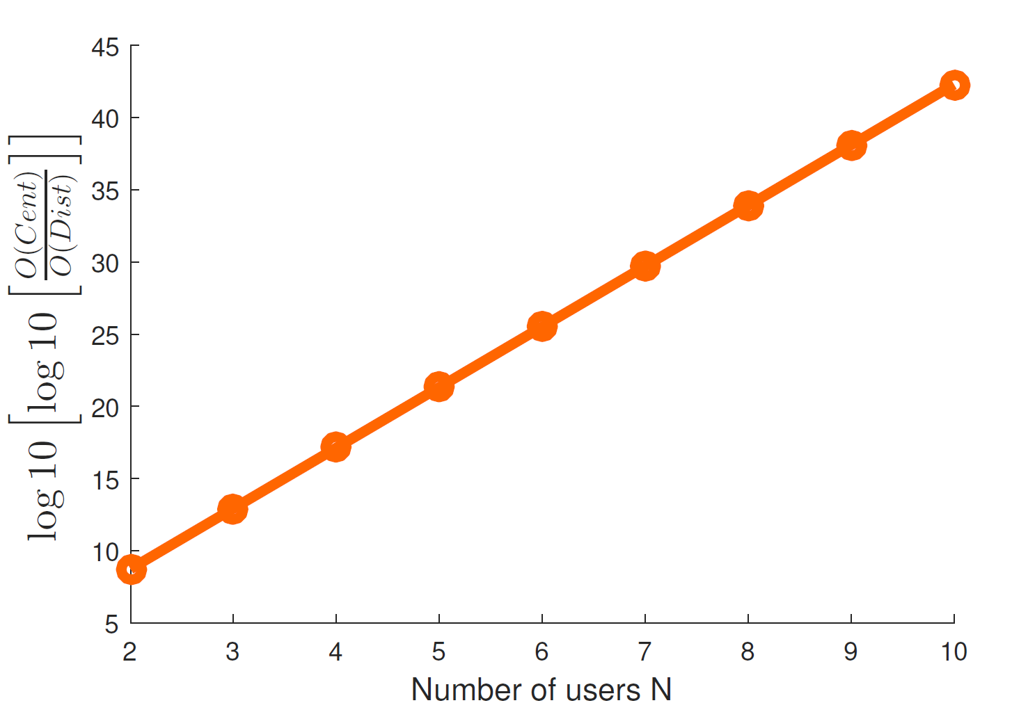
Before evaluating the performance of our relay selection policies, we show the motivation behind these approximations. In fact, we illustrate in figure 5 and 5 how the suggested algorithms highly reduce the computation complexity of the exact solution of the CPOMDP problem. For a single MU scenario and relays, we plot in figure 5 the of the complexity ratio between the exact solution and the proposed CPBVI solution (i.e. given in V-B) as function of the number of possible regions (i.e. called states). This shows that exact solution for of realistic sizes CPOMDP is unfeasible .
In addition, the exponential number of actions motivated us to propose a greedy design of the CPBVI algorithm that avoids the study of all the possible actions. We consider possible states and we plot in figure 5 the complexity ratio between the CPBVI solution and its greedy alternative (i.e. given in V-C) as function of the number of the potential relays . This figure shows that, even for a small number of potential relays , we can reduce the complexity of a factor of .


Moreover, we evaluate the performance of the greedy GCPBVI algorithm (given in V-C) compared to the CPBVI scheme (given by V-B). Indeed, the comparison is done in terms of the average cumulative reward, cost and EE of both CPBVI and GCPBVI relay selection solutions. For this comparison, we consider the following simple scenario: single MU with potential relays and times rectangular regions (i.e. states). Figure 9 verifies that the GCPBVI almost return the same average cumulative reward as the CPBVI algorithm. Both solutions have an average cumulative cost that is lower than the cost threshold given in I. Therefore, similar average cumulative energy efficiency is deduced for both algorithms.


VII-B2 D2D relaying performance
Recall that the aim of this work is to enhance the performance of cellular networks. Thus, we consider the throughput as the performance metric to study and show how implementing the proposed relay selection policy can improve the throughput of cellular networks. We consider the single MU scenario with relays and regions and we show the results of both scenarios: with and without D2D relaying. For different speeds of state changing , we plot in figure 10 the histogram of the average cumulative reward of both scenarios with and without D2D relaying. In the scenario where D2D is enabled we apply the proposed GCPBVI based relay selection algorithm. The speed in this figure illustrates the velocity of the relay in moving between the regions. Hence, a speed is modeled by considering a transition matrix of . Figure 10 shows that we can gain up to percent in terms of throughput by deploying our policy of relay selection in a cellular network. We note a slow decreasing in the throughput when the speed of the relays increases.

VII-C Multi-MU scenario
We consider the case of multiple MU s in the network. Both centralized and distributed relay selection policies were proposed. For evaluating these algorithms we consider locations in the network and we study the complexity as well as the performance of both distributed and centralized relay selection solutions.
VII-C1 The Performance of the Distributed Approach
In figure 13, the complexity of the centralized solution for multi-MU scenario (given in VI-A) is compared to that of the distributed relay selection solution (given in VI-B). The choice of developing a low complexity distributed approach for the multi-MU scenario is validated in figure 13. Indeed, the complexity reduction that the distributed approach offers is proportional to both the number of MU and the number of relays . As an example, the distributed approach reduces the complexity up to times compared to the centralized one in a realistic scenarios of relays and users.
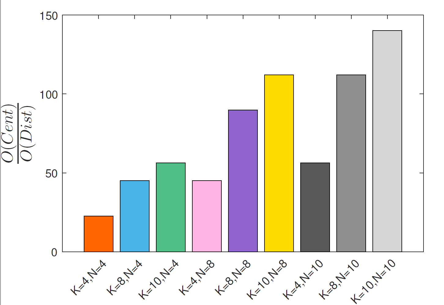
The distributed approach reduces the computational complexity while satisfying a performance close to the centralized one. From figure 17 to figure 17, the performance of the distributed approach is compared to the centralized one. Similarly to the single MU case, the comparison is done in terms of the average cumulative reward, cost and EE of both distributed and centralized solutions. For this comparison, a simple scenario of and is considered. Figure 17 verifies that the low complexity distributed approach almost return the same average cumulative reward as the centralized one. Moreover, both centralized and distributed solutions verify the required cost constraints for each MU (i.e. average cumulative cost lower than the cost threshold given in I). In result, similar average cumulative energy efficiency is deduced for both algorithms. We deduce, that applying distributed relay selection induces interesting performance enhancement of the network with a low computational complexity compared to the centralized approach.


VII-C2 D2D Relaying Performance
We show how implementing the proposed relay selection policy can improve the throughput of cellular networks. We consider the multiple MU s scenario with , discovered relays and regions. For different speeds of state changing , we plot in figure 17 the histogram of the average cumulative reward per MU for both scenarios with and without D2D relaying. In the scenario where D2D is enabled we apply the proposed GCPBVI based relay selection algorithm. The speed in this figure illustrates the velocity of the relays in moving between the regions. Hence, a speed is modeled by considering a transition matrix of . Each MU applies, in a distributed manner, the relay selection policy proposed in V-C. Figure 17 shows that, in average, a MU can gain up to percent of throughput by deploying our policy of relay selection in a cellular network. We note a slow decreasing in the throughput when the speed of the relays increases.
VIII Simulation Results
We have developed a 3rd Generation Partnership Project (3GPP) compliant system level simulator that supports DL, UL and D2D communications. We describe the details of the simulations’ settings in appendix E. In this section we describe the D2D relaying scenario that has been implemented in the simulator and we evaluate the gain that our proposed relay selection policy achieves in a simulated cellular network.
VIII-A Scenario
To complete the results of this paper, we simulate the scenario presented in the flow chart 18. The performance of D2D relaying is evaluated separately for UL and DL scenarios. In this report, we will only present the results corresponding to the DL case for lack of space; however, we would like to note that similar results were evaluated for the UL scenario. The initialization phase of the simulations consists of filling the simulation’s parameters described in E and then generating the cellular network (BS, UE s, received power map, traffic generation etc.). We denote by the number of users and the number of relays generated in each macro cell of the network. The mobility model of the relays is the one considered in the numerical section VII. We use to denote the speed of the relays. (i.e. transition matrix ).
The three main blocks of the simulated scenario are the following: (i) relays discovery where each user discovers nearby relays, (ii) relays selection where each user selects the relays that will ensure the transmission of its traffic (none of the relays is selected if the user found it more beneficial to have traditional cellular communications) and (iii) transmission where a user is scheduled in order to transmit its data (i.e. either in a direct way or through relays). With a periodicity of s, each user runs its discovery process from which it deduces nearby devices. The relays move from a region to another (among the possible regions of each cell) with a time-scale of s. The relay selection decision is taken with the same periodicity . Each TTI, the fast fading is updated for all cellular and D2D communications. The allocation of cellular and D2D resources is done at the TTI scale. After data transmission, if the whole user’s file is transmitted then a new file is generated according to the FTP2 model described in E.
We denote by the simulation duration of TTI s and MHz the bandwidth of the cellular network. The three metrics that are considered for studying the performance of the proposed relay selection policy are the following:
- •
Cumulative Distribution Function (CDF) of the Signal-to-Interference-plus-Noise Ratio (SINR) which reflexes the coverage area enhancement due to D2D relaying in cellular network.
- •
If [bits] is the amount of data transmitted by all the users then the first throughput criteria (i.e. from the network point of view) is computed as follows:
(34) where is the average number of users that are waiting to be served at a given TTI.
- •
If is the number of files that have been transmitted with the throughput at which the was transmitted, then the second throughput criteria (i.e. from the user’s point of view) is computed as follows:
(35)

In the following results, the considered reward criteria is the bit-rate which is deduced from the SINR based on the SINR-throughput mapping described in E. In addition, the cost criteria is given by the relays’ transmission power. Since a power control mechanism is applied to UL and D2D communications, the relays’ transmission power will depend on their channel conditions (i.e. SINR). The cost threshold that each user should not exceed is equal to W.
VIII-B Results
We consider the case of DL communications aided by D2D relaying. The relay selection algorithm implemented is the one described in V-C. The performance of this scenario is given as function of the number of relays and the number of users existing in each macro cell. We show in figure 20 that enabling D2D relaying improves the SINR of DL communications. Moreover, we study the effect of the number of relays on the performance of DL communications. For this aim, we consider users per cell and we plot both throughput metrics (i.e. and from equations 34 and 35) as function of the number of relays (see figure 20). This result illustrates that more the number of relays increases more the gain achieved by D2D relaying is higher. However, one can see that without considering large number of relays, the D2D relaying can attain important gain in terms of spectral efficiency of DL communications.


In addition, we compare between both scenarios with and without D2D relaying as function of the number of users dropped in each cell. We consider a scenario with relays per cell. We show in 21 that for different values of , the spectral efficiency of DL communications increases due to the deployment of our proposed algorithm of relay selection policy. However, in this figure it is not visible for the reader how much the spectral efficiency is increased. Therefore, for different values of , we present in 22 the relative gain achieved by both and (i.e. given in equations 34 and 35) due to the implementation of our proposed algorithm of relay selection. A spectral efficiency enhancement of more than is recorded.


IX Conclusion
Finding the optimal relay selection policy is a challenging problem especially when the mobility of the relays is considered. In this chapter, we have developed a dynamic relays selection strategy that maximizes a certain performance metric of the cellular networks while guaranteeing some cost constraints. A CPOMDP problem has been formulated and its complexity is discussed. Thus, a greedy GCPBVI algorithm is addressed for achieving a low-complexity and close to optimal solution for the problem. Numerical results show the advantage of such approximation in reducing the problem complexity and prove the performance gain that such solution provides to mobile networks. Our claims are verified by implementing the suggested relay selection scheme in a system-level simulator of cellular networks.
Appendix A Proof of theorem V.4
The following definition and lemma are used for proving theorem V.4.
Definition A.1.
The distance function of relay with transition probability and stationary distribution is defined as follows:
| (36) |
Lemma A.2.
From [24], the distance function of relay verifies the following properties:
- •
with the highest eigenvalue of the matrix and the lowest component of the stationary distribution corresponding to .
- •
The density of a belief set is given by:
For any reachable belief point of relay , there exists an integer and a state such that . The construction of the belief set induces that in the equation above can be written as with the integer and the initial state of relay .
Appendix B Proof of theorem V.5
The studied CPOMDP of horizon and an initial state achieves an error bound of when and (see equation (19)) are lower than . Limiting the belief set to generates the following errors on the value functions:
| (39) |
and
| (40) |
with ; .
Appendix C Proof of theorem V.6
Please note that we consider the reward -function as an example. By analogy, we can deduce the same property for the cost -function. In the following, we define the discrete derivativeof a relay knowing that an action set (corresponding to action ) is taken:
| (41) |
is non-negative, monotone and submodular in if the discrete derivative of the -function verifies the following:
| (42) |
and
| (43) |
Considering the reward model (1), the discrete derivative is computed as follows:
Since the total reward model, given by equation (1), is equal to the sum of the reward of each selected relay, then the difference will be limited to the reward of relay as follows:
where is the observation of the state of relay between and epochs, the belief vector of relay at epoch , the belief vector of relay after an observation between and epochs. In order to prove the properties (42) and (43) and deduce by that the submodularity of the -function, we compute for the following two cases:
- •
- •
Relay has been chosen by the policy at epoch : in this case, the decision maker observes the state of relay : . Thus,
The second term since relay has not been chosen between and epochs. In addition, the fourth term since relay has been chosen at epoch . Therefore, the policy will have the same value for both and . Thus,
Thus,
Lemma C.1.
For a relay , the two following statements are verified by induction:
- –
if then
- –
if then
- –
Since the discrete derivative verifies the properties (42) and (43) for the two possible cases studied above; theorem V.6 is deduced.
Appendix D Proof of theorem V.7
The proof is done by induction. We start by verifying equation (27) for . We recall that:
and
Based on the results given in [25], the greedy maximization algorithm achieves a approximation of the exact solution. Thus, . Now, we assume that equation (27) is verified for and prove that it remains verified for .
Based on the definition of function (i.e. equation (15)), we deduce:
| (44) |
We use the following notations where all the maximization are done under cost constraint:
- •
- •
- •
- •
Thus,
Given that -function is submodular and constrained to a modular , then results shown in [25] gives:
From the definition of we know that for all including . Therefore,
For equation (44), . Thus:
Given that function is submodular and constrained to a modular , then as shown in [25]:
We deduce that:
Therefore, theorem V.7 is deduced by induction.
Appendix E Simulation Settings
We have developed a LTE system level simulator that considers DL, UL and D2D features. This simulator is mainly used for evaluating the performance of D2D communications. In particular, we expose the results of implementing the proposed relay selection scheme into the developed system level simulator. In this section, we describe the different characteristics of this system level simulator.
Layout
In the LTE system level simulator, we assume a carrier frequency of GHz and a bandwidth of MHz. We consider an hexagonal grid with tri-sector macro sites. hexagonal cells are formed as illustrated in figure 23. Wrap-around is deployed to avoid border effects and all the cells are supposed synchronized.
Two urban macro scenarios are considered with an Inter-Site Distance (ISD) of m: (i) option : all the users are outdoor and (ii) option : with one RRH/Indoor Hotspot per cell (see section A.2.1.1.5 in [26] for more details about RRH/Indoor Hotzone ). Unless specified otherwise, we implement the layout parameters specified for 3GPP case in table A.2.1.1-1 of [26].

Users drop
The details concerning the users’ drop considered in the simulator are given in table A.2.1.1-1 of [27]. We give a brief description in the sequel. For layout option , all the users are outdoor and they are randomly and uniformly dropped throughout the macro geographical area. For layout option , of the users are randomly and uniformly dropped within the indoor building of each cell and the remaining fraction of users are randomly and uniformly dropped throughout the macro geographical area. We consider of the users outdoor and indoor. This can be guaranteed by considering some of the users that are dropped outdoor as virtual indoor users. We assume the following constraints on the building and users drops: m as the minimum distance between two users, m as the minimum distance between a user and the BS, m as the minimum distance between the building center and the BS. In order to illustrate these two layouts, an example for UE s is given in figure 26.


Channel Model
For cellular communications, we consider the antenna pattern (horizontal and vertical) specified for 3GPP case 1 and detailed in table A.2.1.1-2 of [26]. An BS antenna gain of dBi and an antenna tilt of characterize the BS. The user is assumed to be equipped with omni-directional antennas. The BS transmission power is dBm (almost W) and the users’ maximum transmission power, i.e. on both UL and D2D, is dBm (almost W).
The distance dependent pathloss for cellular communications (UL and DL) corresponds to the macro-to-UE model for 3GPP case 1 given in table A.1.1.2-3 of [26]. Hence, for a distance Km between the BS and the UE, the cellular pathloss is given in dB as follows:
In addition, the LOS probability of both UL and DL communications is the one specified in table A.1.1.2-3 of [26] for the 3GPP case 1. Thus, for a distance Km between the BS and the UE, the LOS probability is given by:
When the user is indoor, then its UL and DL communications suffer from a penetration loss of mean dB.
For cellular links, both UL and DL, we consider large scale shadowing caused by the geographical irregularities of the environment due to the presence of obstacles between the BS and the UE (e.g. buildings). In this simulator, shadowing is modeled as a zero-mean Gaussian random variable, with standard deviation dB. A shadowing map is constructed for each site in the network with a precision of Pixels. Both spatial and time correlation exist between the shadowing maps of different sites with a correlation distance of m and a time correlation of s. The shadowing maps are updated frequently with a periodicity of s. The details of the shadowing model is described in the appendix A of [28].
For the case of D2D links, the distance dependent pathloss, the LOS probability, the penetration loss and the shadowing settings are given in table A.2.1.2 of [27] (i.e. for different scenarios outdoor-to-outdoor, outdoor-to-indoor and indoor-to-indoore). The antenna gain for D2D communications is considered dBi (i.e. given in table A.2.1.1-1 of [27]).
For cellular communications, the fast fading has a Rayleigh distribution, i.e. square root of the sum of the squares of two normal distribution random variables and . The fast fading is assumed to vary according to a Gauss-Markov model. If is the speed traveled by a user then the correlation coefficient is given by:
| (45) |
where the carrier frequency and the speed of light. We apply the correlation on the two component of the fast fading as follows:
where and are two random variables with normal distribution and the as a correction that is added to guarantee a fast fading of average one.
In addition, and are generated based on the existing spatial correlation between the fast fading coefficients. We consier the correlation matrix defined in table B.2.2.1 of [29] with (i.e. low spatial correlation). In order to introduce spatial correlation into the channels coefficients according to a specific correlation matrix , we consider a vector of Multiple Input Multiple Output (MIMO) uncorrelated channel matrix (i.e. random variables with normal distribution) and multiply it by the lower triangular matrix corresponding to the Cholesky factorization of the correlation matrix .
The same model of fast fading is applied to D2D communications. The only difference is that the velocity in equation 45 is modified as specified in section A.2.1.2.1 of [27].
The noise parameters are the following: thermal noise dbm/Hz, the BS noise figure dB, UE noise figure dB and D2D noise figure dB.
On the UL, a power control is installed in order to reduce the power emitted by the users and limit by that the interference between neighbor cells. For a pathloss between the UE and the BS (i.e. taking into account the distance dependent pathloss, penetration loss, antenna pattern and shadowing loss), the user transmits at the following power:
where is the maximum user’s transmission power, dBm is the target received power at the BS and is the compensation factor. The same mechanism of Power control is applied for D2D communications.
We consider LTE codebook-based precoding for enabling transmit diversity mode. We assume that a single layer data stream is transmitted via two antennas. The following transmission schemes are simulated: MIMO for DL and MIMO for both UL and D2D communications. The precoding at the transmitter is done by choosing the precoding vector among II that maximizes the received power.
| Codebook index | Rank | Rank |
|---|---|---|
| 0 | ||
| 1 | ||
| 2 | ||
| 3 |
Link curves
The SINR maps of the DL and UL channel models considered in the simulator are respectively given in figures 28 and 30. Based on a link-level simulator, we deduce the mapping between the SINR and the rate (Kbits/s/Hz) for both DL (see figure 28) and UL (see figure 30) communications. We deduce the amount of data transmitted at each allocated Resource Block (RB). The UL link adaptation is applied to D2D communications; thus the UL SINR-rate mapping is considered for D2D links.


Traffic Model
Considering a fix number of users, FTP2 model of traffic given in section A.2.1.3 of [26] is assumed (see figure 31). A DL file size of MBytes and an UL file size of Mbytes are considered. An exponential reading time of parameter separates the end of a file download and the arrival of the next file (i.e. the mean of is s).

Scheduling
We consider a round-robin scheduler that serves the users in a cycle way and independently of their radio conditions. At a given time-slot, only one UE is scheduled (i.e. all the available RB s are allocated to the selected UE). Since overlay D2D is assumed and the UL resources are often less utilized than the DL resources, we dedicate of the UL resources for D2D communications.
D2D discovery
The discovery process allow a device to discover nearby users with whom D2D communication can be established. We implement the discovery process described in [27] and validate it by comparing our results to the one given in [27]. The following scenario is considered for evaluating the implementation of the discovery procedure. In each cell, among the created macro cells, UE s are dropped using one of the two dropping procedures (i.e. options 1 and 2) described in E. The SINR of D2D links is illustrated in figure 32 and is compared to UL and DL SINR.

For each discovery period of s, a limited number of subframes (i.e. TTI s) are dedicated for the discovery process. Indeed, one RB pair is randomly allocated to each device among all the resources available in the discovery subframes. Therefore, each user will transmit its discovery signal on its allocated physical RB s. When this discovery signal is decoded by a nearby user then the latter considers the device generating the discovery signal as a discovered user (i.e. minimum association received power is dBm). Considering half duplex devices, then users transiting at the same TTI cannot discover each other. An in-band emissions described in table A.2.1.5-1 of [27] is evaluated in each non-allocated RB with as W,X,Y,Z parameters .
For evaluating the discovery scheme described above, the two following metrics are considered and compared to those given in [27].
- •
- •


References
- [1] Y. Chen, P. Martins, L. Decreusefond, F. Yan, and X. Lagrange, “Stochastic analysis of a cellular network with mobile relays,” in 2014 IEEE Global Communications Conference, Dec 2014, pp. 4758–4763.
- [2] J. Liu and N. Kato, “Device-to-device communication overlaying two-hop multi-channel uplink cellular networks,” in Proceedings of the 16th ACM International Symposium on Mobile Ad Hoc Networking and Computing, ser. MobiHoc ’15. New York, NY, USA: ACM, 2015, pp. 307–316. [Online]. Available: http://doi.acm.org/10.1145/2746285.2746311
- [3] K. Vanganuru, S. Ferrante, and G. Sternberg, “System capacity and coverage of a cellular network with d2d mobile relays,” in MILCOM 2012 - 2012 IEEE Military Communications Conference, Oct 2012, pp. 1–6.
- [4] H. Lin, D. Gu, W. Wang, and H. Yang, “Capacity analysis of dedicated fixed and mobile relay in lte-advanced cellular networks,” in 2009 IEEE International Conference on Communications Technology and Applications, Oct 2009, pp. 354–359.
- [5] L. Babun, A. . Yürekli, and . Güvenç, “Multi-hop and d2d communications for extending coverage in public safety scenarios,” in 2015 IEEE 40th Local Computer Networks Conference Workshops (LCN Workshops), Oct 2015, pp. 912–919.
- [6] R. Atat, L. Liu, N. Mastronarde, and Y. Yi, “Energy harvesting-based d2d-assisted machine-type communications,” IEEE Transactions on Communications, vol. 65, no. 3, pp. 1289–1302, March 2017.
- [7] M. Hasan and E. Hossain, “Distributed resource allocation for relay-aided device-to-device communication under channel uncertainties: A stable matching approach,” IEEE Transactions on Communications, vol. 63, no. 10, pp. 3882–3897, Oct 2015.
- [8] J. M. B. da Silva, G. Fodor, and T. F. Maciel, “Performance analysis of network-assisted two-hop d2d communications,” in 2014 IEEE Globecom Workshops (GC Wkshps), Dec 2014, pp. 1050–1056.
- [9] D. Niyato and P. Wang, “Optimization of the mobile router and traffic sources in vehicular delay-tolerant network,” IEEE Transactions on Vehicular Technology, vol. 58, no. 9, pp. 5095–5104, Nov 2009.
- [10] Z. Zhang, X. Chen, Y. Zhang, C. Zhong, and W. Wang, “Energy-efficient opportunistic packet scheduling in mobile relay systems,” IEEE Transactions on Vehicular Technology, vol. 65, no. 7, pp. 5327–5336, July 2016.
- [11] Y. Wei, F. R. Yu, and M. Song, “Distributed optimal relay selection in wireless cooperative networks with finite-state markov channels,” IEEE Transactions on Vehicular Technology, vol. 59, no. 5, pp. 2149–2158, Jun 2010.
- [12] S. Yun, K. Lee, S. Park, and J. K. Choi, “Energy efficient relay selection scheme with drx mechanism in 3gpp lte network,” in 2013 International Conference on ICT Convergence (ICTC), Oct 2013, pp. 6–11.
- [13] T. Kim and M. Dong, “An iterative hungarian method to joint relay selection and resource allocation for d2d communications,” IEEE Wireless Communications Letters, vol. 3, no. 6, pp. 625–628, Dec 2014.
- [14] R. Ma, Y. Chang, H. Chen, and C. Chiu, “On relay selection schemes for relay-assisted d2d communications in lte-a systems,” IEEE Transactions on Vehicular Technology, vol. 66, no. 9, pp. 8303–8314, Sept 2017.
- [15] X. Ma, R. Yin, G. Yu, and Z. Zhang, “A distributed relay selection method for relay assisted device-to-device communication system,” in 2012 IEEE 23rd International Symposium on Personal, Indoor and Mobile Radio Communications - (PIMRC), Sept 2012, pp. 1020–1024.
- [16] Y. Li, P. Wang, D. Niyato, and W. Zhuang, “A dynamic relay selection scheme for mobile users in wireless relay networks,” in 2011 Proceedings IEEE INFOCOM, April 2011, pp. 256–260.
- [17] Y. Li, Y. Hou, Z. Huang, and Y. Wei, “Cooperative relay selection policy using partially observable markov decision process,” in 2011 Seventh International Conference on Natural Computation, vol. 1, July 2011, pp. 508–512.
- [18] Y. Polyanskiy, H. V. Poor, and S. Verdu, “Channel coding rate in the finite blocklength regime,” IEEE Transactions on Information Theory, vol. 56, no. 5, pp. 2307–2359, May 2010.
- [19] R. D. Smallwood and E. Sondik, “The optimal control of partially observable markov processes over a finite horizon,” Operations research, vol. 21, no. 5, pp. 1071–1088, 1973.
- [20] A. R. Cassandra, “Exact and approximate algorithms for partially observable markov decision processes,” 1998.
- [21] J. D. Isom, S. P. Meyn, and R. D. Braatz, “Piecewise linear dynamic programming for constrained pomdps,” in AAAI, vol. 1, 2008, pp. 291–296.
- [22] D. Kim, J. Lee, K. E. Kim, and P. Poupart, “Point-based value iteration for constrained pomdps,” in IJCAI, 2011, pp. 1968–1974.
- [23] J. Pineau, G. Gordon, and S. Thrun, “Point-based value iteration: An anytime algorithm for pomdps,” in Proceedings of the 18th International Joint Conference on Artificial Intelligence, ser. IJCAI’03. San Francisco, CA, USA: Morgan Kaufmann Publishers Inc., 2003, pp. 1025–1030. [Online]. Available: http://dl.acm.org/citation.cfm?id=1630659.1630806
- [24] D. A. Levin and Y. Peres, Markov chains and mixing times. American Mathematical Soc., 2017, vol. 107.
- [25] M. Sviridenko, “A note on maximizing a submodular set function subject to a knapsack constraint,” Oper. Res. Lett., vol. 32, pp. 41–43, 2004.
- [26] TR36814, “Evolved universal terrestrial radio access (e-utra); further advancements for e-utra physical layer aspects release 9 v9.2.0 2017,” 2017.
- [27] TR36834, “Technical report 3GPP TR 36.843: Study on LTE Device-to-Device proximity services v12.0.1 2014,” 2014.
- [28] N. Abbas, “Design and performance of coordination schemes in cellular networks,” Theses, Télécom ParisTech, Nov. 2016. [Online]. Available: https://pastel.archives-ouvertes.fr/tel-01618909
- [29] TR36803, “Evolved universal terrestrial radio access (e-utra); user equipment (ue) radio transmission and reception v 1.1.0 2008,” 2008.
The authors would like to thank…
| Rita Ibrahim received the B.E. degree from Telecom-Paristech, France, and Lebanese University, Lebanon, in 2015, and the M.Sc. degree in advanced communication networks jointly from Ecole Polytechnique and Telecom-Paristech, France, in 2015. She obtained a PhD degree from CentraleSupélec, France, in 2019. She is currently a research engineer in Orange Labs, France. Her current research interests include analytic modeling and performance evaluation of cellular networks, stochastic network optimization, and radio access technologies for 5G networks. |
| Mohamad Assaad received the MSc and PhD degrees (with high honors), both in telecommunications, from Telecom ParisTech, Paris, France, in 2002 and 2006, respectively. Since 2006, he has been with the Telecommunications Department at CentraleSupélec, where he is currently a professor and holds the TCL Chair on 5G. He is also a researcher at the Laboratoire des Signaux et Systèmes (L2S, CNRS). He has co-authored 1 book and more than 100 publications in journals and conference proceedings and serves regularly as TPC member or TPC co-chair for top international conferences. He is an Editor for the IEEE Wireless Communications Letters and the Journal of Communications and Information Networks. He has given in the past successful tutorials on 5G systems at various conferences including IEEE ISWCS’15 and IEEE WCNC’16 conferences. His research interests include 5G networks, MIMO systems, mathematical modelling of communication networks, stochastic network optimization and Machine Learning in wireless networks. |
| Berna Sayrac is a senior research expert in Orange Labs. She received the B.S., M.S. and Ph.D. degrees from the Department of Electrical and Electronics Engineering of Middle East Technical University (METU), Turkey, in 1990, 1992 and 1997, respectively. She worked as an Assistant Professor at METU between 2000 and 2001, and as a research scientist at Philips Research France between 2001 and 2002. Since 2002, she is working at Orange Labs. Her current research activities and interests include 5G radio access and spectrum. She has taken responsibilities and been active in several FP7 European projects, such as FARAMIR, UNIVERSELF, and SEMAFOUR. She was the technical coordinator of the Celtic+ European project SHARING on self-organized heterogeneous networks, and also the technical manager of the H2020 FANTASTIC-5G project. Currently, she is the coordinator of the research program on RAN design and critical communications in Orange. She holds several patents and has authored more than fifty peer-reviewed papers in prestigious journals and conferences. She also acts as expert evaluator for research projects, as well as reviewer, TPC member and guest editor for various conferences and journals. |