跳到论文正文
W Papers独立论文阅读器 arXiv:1905.02372 论文正文 计算阅读时间 · 0%
引用这篇论文根据当前论文元数据生成,正式投稿前建议核对。


License: CC BY 4.0
arXiv:1905.02372v3 [physics.gen-ph] 13 Dec 2023

[This is the Accepted Manuscript version of an article accepted for publication in Journal of Physics Communications. IOP Publishing Ltd is not responsible for any errors or omissions in this version of the manuscript or any version derived from it. This Accepted Manuscript is published under a CC BY license. The Version of Record is available online at https://doi.org/10.1088/2399-6528/ad0649.]

  A new method that automatically regularizes

scattering amplitudes

Nagabhushana Prabhu11 1 prabhu@purdue.edu

Purdue University, West Lafayette, IN 47907

Abstract

We present a new regularization procedure called autoregularization. The new procedure regularizes the divergences, encountered previously in a scattering process, using the intrinsic scale of the process. We use autoregularization to calculate the amplitudes of several scattering processes in QED and compare the calculations with experimental measurements over a broad range of center-of-momentum energies (≲\lesssim MeV to ≳\gtrsim 200 GeV). The calculated amplitudes are found to be in good agreement with experimental data22 2 Specifically, the O⁡(α)O(\alpha) correction to electron’s gyromagnetic ratio predicted by autoregularization agrees with experimental measurement to within 0.06% (Section 3.1), which is to be compared to Schwinger’s O⁡(α)O(\alpha) correction which agrees with experimental measurement to within 0.15%0.15\%; the O⁡(α)O(\alpha) estimate of the Lamb shift predicted by autoregularization agrees with the experimental measurements to within 0.33%0.33\% (see Section 3.2); the running fine structure constant predicted by autoregularization at O⁡(α)O(\alpha) agrees with the prediction of cutoff regularization to within 0.8% over one to four orders of magnitude above the electron’s mass scale (Section 3.3); the tree-level prediction of autoregularization for Compton scattering is in better agreement with experimental data than the prediction of the well-known Klein-Nishina formula by about 4.02% ( Section 3.5.1); the tree-level predicition of autoregularization for pair annihilation at center-of-momentum energy of 206.671 GeV agrees with the experimental data about 0.67 % better than the prediction of the standard QED ( Section 3.5.2).. To test autoregularization in a non-Abelian gauge theory, we calculate the QCD coupling constant at 1-loop and show that, like the known regularization schemes, autoregularization also predicts asymptotic freedom in QCD. Finally, we show that the vacuum energy density of the free fields in the Standard Model, calculated using autoregularization, is smaller than the current estimate of the cosmic critical density.

1 Introduction

Several regularization schemes have been used for renormalizing scattering amplitudes in quantum field theory. A regularization scheme introduces an arbitrary energy scale into the renormalization process—such as the cutoff scale in Wilson’s renormalization, the masses of fictitious particles in Pauli-Villars regularization or the energy scale that is introduced in dimensional regularization to consistently extend the action to arbitrary spacetime dimension [1, 2, 3, 4, 5, 6, 7, 8, 9]. In all cases the regularization schemes, as well as the energy scales they introduce, are independent of the kinematics of the scattering process of interest.

On the other hand every scattering process or phenomenon has an intrinsic ‘energy’ scale that provides a natural candidate for the energy scale needed in regularization. For example, the Mandelstam variables provide Lorentz-invariant kinematic ‘energy’ scales that are intrinsic to the scattering process under consideration. One can construct a customized regularization scheme for each scattering process or phenomenon using the intrinsic ‘energy’ scale of the scattering process or the phenomenon itself, rather than an energy scale introduced by fiat. Regularization that uses the intrinsic ‘energy’ scale of the very process or phenomenon being regularized will be called autoregularization. We present such an autoregularization scheme in the following discussion.

A key new feature of autoregularization is that in it the representations of free fields depend on the scattering process or phenomenon of interest. Specifically, the creation and annihilation operators of free fields are scaled by the so-called Gibbs factors33 3 The term is borrowed from the formalism of the Grand Canonical Ensemble, in which the Gibbs factor suppresses the fluctuation of any system that is in thermal and diffusive equilibrium with a reservoir. See Appendix A., which depend on the Lorentz-invariant intrinsic scale of the scattering process or phenomenon under consideration. As a result of the above scaling the scattering amplitudes are rendered naturally divergence-free at all orders of perturbation theory. Autoregularization is described in the next section.

As preliminary test of autoregularization we compare its predictions at 1-loop with the experimental measurements of the anomalous magnetic moment of the electron44 4 The O⁡(α)O(\alpha) correction to electron’s anomalous magnetic moment, aea_{{}_{e}}, calculated using autoregularization, is closer to experimental data than Schwinger’s O⁡(α)O(\alpha) prediction [12]. aea_{{}_{e}} has been calculated previously up to the tenth order [13], and the theoretical calculations are found to agree with experimental measurements [14, 15] up to the tenth decimal place. Calculation of higher order corrections of aea_{{}_{e}}, using autoregularization, will be the focus of follow-up work. and Lamb shift. We also compare the the running fine structure constant predicted by autoregularization at 1-loop with the corresponding prediction of the cutoff regularization at momentum transfer scales up to 10410^{4} times the electron mass scale. At the tree-level, we compare the predictions of autoregularization with the experimental measurements of Compton scattering (at ∼\sim MeV; Friedrich and Goldhaber [10]) and e+−e−e^{+}-e^{-} pair annihilation (at ∼\sim 206 GeV; ALEPH collaboration [11]). The predictions of autoregularization are found to be in good agreement with the experimental data and with the prediction of the cutoff regularization.

The above tests pertain to scattering processes in QED, an Abelian gauge theory. To test autoregularization in a non-Abelian gauge theory we consider the running of the QCD coupling constant. Known regularization schemes predict the remarkable phenomenon of asymptotic freedom in QCD. We calculate the QCD coupling constant at 1-loop and confirm that autoregularization also predicts asymptotic freedom in QCD.

Following the the above tests, we use autoregularization to compute the vacuum energy density of the free fields in the Standard Model, and obtain a value smaller than the current estimate of the critical density.

The paper is organized as follows. Following a description of autoregularization in the next section, we use it to calculate the amplitudes of selected scattering processes in Section 3. We compute the 1-loop correction to electron’s anomalous magnetic moment in Section 3.1 and the Lamb shift in Section 3.2. In Section 3.3 we use autoregularization  to compute the running of the fine structure constant at 1-loop—for momentum transfer scales that are up to four orders of magnitude above the electron’s rest mass scale. Section 3.1 – Section 3.3 contain the summaries of the above calculations, with the underlying details deferred to Appendices B–D. In Section 3.4 we calculate the running of the QCD coupling constant and show that autoregularization also predicts that QCD is an asymptotically free theory. In Section 3.5 we calculate tree-level amplitudes of two scattering processes. In Section 3.5.1 we compare the tree-level prediction of autoregularization for Compton scattering with the experimental data and with the prediction of the Klein-Nishina formula. In Section 3.5.2 we compare the tree-level predictions of both autoregularization and the standard QED with the experimental data for pair annihilation. In Section 4, we use autoregularization  to calculate the vacuum energy density of the free fields in the Standard Model. Section 5 contains the concluding remarks. Unless specified otherwise we work in natural units.

2 Description of and formalism for autoregularization

In a scattering process, particles of a quantum field can be created or annihilated and momentum can be transferred to or from the particles of the field. That is, particles and energy can flow into or out of a quantum field during scattering. Hence, one can view a quantum field as a system that is in thermal and diffusive equilibrium with a reservoir made of the other quantum fields that participate in the scattering process of interest.

The statistical behavior of a system that is in thermal and diffusive equilibrium with a reservoir is well-described, in statistical mechanics, by the Grand Canonical Distribution (GCD), first derived by J.W. Gibbs [16, 17]. GCD states that the probability of a fluctuation that puts the system in a state with a certain particle number and energy EE is proportional to the Gibbs factor, which decreases exponentially with EE. The stochastic description of fluctuations of a system, given by GCD, provides a natural paradigm for describing stochastic fluctuations of a quantum field, and by extension stochastic scattering processes.

Modeled after the GCD, autoregularization constrains the probabilities of fluctuations of quantum fields by including Lorentz-invariant Gibbs factors55 5 The Lorentz-invariant (frame-independent) Gibbs factors, described in Section 2.2, differ slightly from the (frame-dependent) Gibbs factors in GCD. With some abuse of notation we use the term “Gibbs factors” for the Lorentz-invariant factors, described in Section 2.2, as well. in the description of quantum fields. Constraining the probabilities of fluctuations of quantum fields with Gibbs factors has the immediate consequence of eliminating divergences from scattering amplitudes, at all orders of perturbation theory. The Lorentz-invariant Gibbs factors are described in Section 2.2 and Appendix A. We begin the discussion by describing how Gibbs factors are included in autoregularization.

Consider a scattering process 𝒫{\cal P} seen by an observer who is at rest in frame ℱ{\cal F}. We seek to calculate the SS-matrix element of the process66 6 Thus we assume that the incoming and outgoing particles in the scattering process, the asymptotic momenta of the incoming and outgoing particles (in some Lorentz frame ℱ{\cal F}), and the Lagrangian governing the particles’ interactions are specified at the outset. Further, we assume that the tree-level Feynman diagrams are connected; that is, we assume that 𝒫{\cal P} does not describe two or more non-interacting scattering processes.. Let ℒ{\cal L} be the Lagrangian that underlies 𝒫{\cal P} and let φ\varphi denote a generic quantum field in ℒ{\cal L}. For simplicity, we assume φ\varphi is a scalar field of mass mm. In autoregularization we scale the creation and annihilation operators in the free-field expansion of φ\varphi (in the interaction picture) with a Lorentz-invariant Gibbs77 7 The discussion in Appendix A clarifies the reason for calling it the Gibbs factor. factor gφg_{{}_{\varphi}} as follows.

φint(x;ℱ,𝒫)\displaystyle\varphi_{{}_{\mbox{\scriptsize int}}}(x;{\cal F},{\cal P}) =\displaystyle= ∫d3​k(2​π)3gφ(k→;ℱ,𝒫){𝐚^(k)e−i​k→​x+𝐚^†(k→)ei​k→​x}\displaystyle\int\displaystyle\frac{d^{3}k}{(2\pi)^{3}}\ g_{{}_{\varphi}}(\uline{\vec{k}};{\cal F},{\cal P})\left\{{\bf\hat{a}}(k)e^{\displaystyle-i\uline{\vec{k}}x}\ +{\bf\hat{a}}^{\dagger}(\vec{k})e^{\displaystyle i\uline{\vec{k}}x}\ \right\} (1)

where 𝐚^{\bf\hat{a}} and 𝐚^†{\bf\hat{a}}^{\dagger} denote the annihilation and creation operators. We follow the convention of underlining a 4-vector to indicate that it is on mass shell. Specifically, k→:=(|k→|2+m2,k→)\uline{\vec{k}}:=(\sqrt{|\vec{k}|^{2}+m^{2}},\vec{k}). φint\varphi_{{}_{\mbox{\scriptsize int}}} remains a solution of the Klein-Gordon equation88 8 We drop the subscript in φint\varphi_{{}_{\mbox{\scriptsize int}}} hereafter.. The creation and annihilation operators of a generic free quantum field–for example, Dirac field or Maxwell field– are similarly scaled by a Gibbs factor and a generic free field satisfies the corresponding Euler-Lagrange equation.

The Gibbs factor, and hence φ\varphi, depends on the scattering process 𝒫{\cal P}. The Gibbs factor is constructed using the Lorentz invariant described below.

2.1 Lorentz-invariant extension of center-of-momentum energy for construction of Gibbs factor

Let ℱ𝒫{\cal F}_{{}_{\cal P}} be a center-of-momentum frame of the scattering process 𝒫{\cal P}. ℱ𝒫{\cal F}_{{}_{\cal P}} is determined up to spatial rotations. Let 𝒰(ℱ𝒫;ℱ){\cal U}({\cal F}_{{}_{\cal P}};{\cal F}) denote the 4-velocity of an observer who is at rest in frame ℱ𝒫{\cal F}_{{}_{\cal P}}, as seen by an observer who is at rest in frame ℱ{\cal F}. Let πφ\pi_{{}_{\varphi}} denote the projection of a momentum 4-vector onto the mass shell of φ\varphi. Specifically, for 4-momentum k:=(k0,k→)k:=(k^{0},\vec{k}),

πφ(k)\displaystyle\pi_{{}_{\varphi}}(k) :⁣=\displaystyle:= (ω⁡(k),k→),ω⁡(k):=[|k→|2+m2]1/2\displaystyle(\omega(k),\vec{k}),\qquad\omega(k):=\left[\,|\vec{k}\,|^{2}+m^{2}\,\right]^{1/2} (2)

where mm is the mass corresponding to the free field φ\varphi. Let Λ(ℱ𝒫,ℱ)\Lambda({\cal F}_{{}_{\cal P}},{\cal F}) denote the Lorentz transformation that maps a 4-momentum in ℱ{\cal F} to a corresponding 4-momentum in ℱ𝒫{\cal F}_{{}_{\cal P}}. Given a 4-momentum kk in ℱ{\cal F}, ξ\xi, defined as

ξφ(k;ℱ,𝒫)\displaystyle\xi_{{}_{\varphi}}(k;{\cal F},{\cal P}) :⁣=\displaystyle:= Λ−1(ℱ𝒫,ℱ)(πφ[Λ(ℱ𝒫,ℱ)k])\displaystyle\Lambda^{-1}({\cal F}_{{}_{\cal P}},{\cal F})\left(\pi_{{}_{\varphi}}\left[\,\rule{0.0pt}{14.0pt}\Lambda({\cal F}_{{}_{\cal P}},{\cal F})k\,\right]\right) (3)

maps kk to an on-mass-shell 4-momentum. Although, ℱ𝒫{\cal F}_{{}_{\cal P}} appears on the right hand side above, it is easy to see that the left hand side is independent of the particular center-of-momentum frame ℱ𝒫{\cal F}_{{}_{\cal P}} that one chooses, and depends only on the process 𝒫{\cal P}. We observe that

Eφ(k;ℱ,𝒫)\displaystyle E_{{}_{\varphi}}(k;{\cal F},{\cal P}) :⁣=\displaystyle:= ξφα(k;ℱ,𝒫)𝒰α(ℱ𝒫;ℱ)\displaystyle\xi^{\alpha}_{{}_{\varphi}}(k;{\cal F},{\cal P})\,{\cal U}_{\alpha}({\cal F}_{{}_{\cal P}};{\cal F}) (4)

is a Lorentz invariant. Setting ℱ=ℱ𝒫{\cal F}\ =\ {\cal F}_{{}_{\cal P}} in (3) we see that in a center-of-momentum frame ℱ𝒫{\cal F}_{{}_{\cal P}}, EφE_{{}_{\varphi}} reduces to

Eφ(k;ℱ𝒫,𝒫)\displaystyle E_{{}_{\varphi}}(k;{\cal F}_{{}_{\cal P}},{\cal P}) =\displaystyle= ω⁡(k)\displaystyle\omega(k) (5)

2.2 Gibbs factor formulas for Fermions and Bosons

Deferring a derivation of the Gibbs factor as well as a discussion of the form of the Gibbs factor to Appendix A, we state the explicit form of the Gibbs factor below. Using the abbreviation Eφ(k):=Eφ(k;ℱ,𝒫)E_{{}_{\varphi}}(k):=E_{{}_{\varphi}}(k;{\cal F},{\cal P}), the Gibbs factor for a field φ\varphi in frame ℱ{\cal F}, for process 𝒫{\cal P}, is defined as

gφ(k;ℱ,𝒫)\displaystyle g_{{}_{\varphi}}(k;{\cal F},{\cal P}) =\displaystyle= {[dφe(Eφ(k)−μφ)/τ−1]1/4,φ: massive boson[dφe(Eφ(k)−μφ)/τ+1]1/4,φ: massive fermion[dφeEφ(k)/τ+τ/Eφ(k)−1]1/4,φ: massless boson\displaystyle\left\{\begin{array}[]{ll}\left[\,\frac{\displaystyle{d_{{}_{\varphi}}}_{{}_{\ }}}{\displaystyle e^{(E_{{}_{\varphi}}(k)-\mu_{{}_{\varphi}})/\tau}-1}\,\right]^{1/4},&\varphi:\mbox{ massive boson}\\ \\ \left[\,\frac{\displaystyle{d_{{}_{\varphi}}}_{{}_{\ }}}{\displaystyle e^{(E_{{}_{\varphi}}(k)-\mu_{{}_{\varphi}})/\tau}+1}\,\right]^{1/4},&\varphi:\mbox{ massive fermion}\\ \\ \left[\,\frac{\displaystyle{d_{{}_{\varphi}}}_{{}_{\ }}}{\displaystyle e^{E_{{}_{\varphi}}(k)/\tau+\tau/E_{{}_{\varphi}}(k)}-1}\,\right]^{1/4},&\varphi:\mbox{ massless boson}\end{array}\right.

dφd_{{}_{\varphi}}, the degeneracy factor, is the number of distinct creation operators in the free field expansion of φ\varphi and its conjugate. For example, the degeneracy factor for an electron is de=4d_{{}_{e}}=4 and for a photon it is dp=2d_{{}_{p}}=2. μφ\mu_{{}_{\varphi}}, the chemical potential of field φ\varphi corresponding to a particle of mass mm and an electric charge99 9 Given that we do not know if neutrinos are Majorana fermions, electric charge is the only conserved charge of interest for the particles involved in the scattering processes that we consider in this paper. However, in scattering processes involving particles that carry other conserved charges, such as the color charge, the definition of chemical potential will likely need to be extended to encompass other conserved charges. of magnitude q​|e|q\,|e| is defined as

μφ\displaystyle\mu_{{}_{\varphi}} =\displaystyle= 9​α​m2​q216​π\displaystyle\sqrt{\displaystyle\frac{9\alpha m^{2}q^{2}}{16\pi}} (12)

in units in which ℏ=c=me=ϵ0=1\hbar=c=m_{{}_{e}}=\epsilon_{{}_{0}}=1. α\alpha denotes the fine structure constant, mem_{{}_{e}}, the rest mass of the electron and the other symbols have the standard meanings. A massless boson is assumed to have vanishing electric charge and thus a vanishing chemical potential. As described after Equation (93), a particle and its antiparticle are stipulated to have equal chemical potentials.

τ𝒫\tau_{{}_{{\cal P}}}, the intrinsic ‘energy’ scale of a scattering process 𝒫{\cal P} with mm incoming particles of momenta p1,…,pmp_{{}_{1}},\ldots,p_{{}_{m}} and nn outgoing particles of momenta q1,…,qnq_{{}_{1}},\ldots,q_{{}_{n}}, is defined as

τ𝒫\displaystyle\tau_{{}_{{\cal P}}} =\displaystyle= maxℐ,𝒥{|kμ​kμ||k=∑i∈ℐpi−∑j∈𝒥qj,}\displaystyle\max_{{\cal I},{\cal J}}\left\{\sqrt{|k_{\mu}k^{\mu}|}\ \left|\ k\ =\ \sum_{i\in{\cal I}}p_{{}_{i}}-\sum_{j\in{\cal J}}q_{{}_{j}},\right.\right\} (13)

where ℐ⊆{1,…,m},𝒥⊆{1,…,n},0<|ℐ|+|𝒥|<m+n{\cal I}\subseteq\left\{1,\ldots,m\right\},{\cal J}\subseteq\left\{1,\ldots,n\right\},0<|{\cal I}|+|{\cal J}|<m+n. τ𝒫\tau_{{}_{{\cal P}}} is abbreviated to τ\tau in (2.2) and in the rest of this section.

It should not be surprising that the Gibbs factor for massless boson is not the limit of the Gibbs factor of a massive boson where the mass → 0\rightarrow\,0. Even in canonical quantization the quantization of the massless Maxwell field cannot be implemented as the massless limit of the quantization of a massive boson field; the quantization of the massless field is a more delicate procedure than the quantization of a massive field. Further a continuous limit is precluded by the fact that massive and massless bosons have different numbers of physical degrees of freedom.

In the other regularization schemes the regularization parameter is driven to a limit (for eg., ϵ=4−d→ 0\epsilon=4-d\rightarrow\,0 in dimensional regularization) and eliminated after regularization is completed. On the other hand, the regularization parameter τ\tau in autoregularization, derived from the kinematics of 𝒫{\cal P}, is not driven to a limit and persists in the calculation.

From the structure of the Gibbs factors we see that, in autoregularization, more energetic processes—that is processes with higher τ\tau—probe deeper into the UV regime (in the sense that they receive greater contributions from high ‘energy’ modes) than less energetic processes. Thus the cutoff is neither sharp nor pre-specified.

The Lorentz invariance of the Gibbs factor follows from the Lorentz invariance of τ,μφ\tau,\mu_{{}_{\varphi}} and Eφ(k)E_{{}_{\varphi}}(k). We note that gφ4g_{{}_{\varphi}}^{4} resembles the Bose-Einstein and Fermi-Dirac distributions for massive boson and fermion fields. Gibbs factor for massless bosons, such as photons, includes a term in the exponent that suppresses infrared divergence.

2.3 Derivation of Feynman propagators for electrons and photons

If the Gibbs factor is set to gφ=1g_{{}_{\varphi}}=1 in (1) one recovers the process-independent representation of the free field, denoted Φ⁡(x)\Phi(x). It is well known that imposing equal-time commutation relations on Φ⁡(x)\Phi(x) and its conjugate momentum is equivalent to imposing commutation relations on the creation and annihilation operators 𝐚^†{\bf\hat{a}}^{\dagger} and 𝐚^{\bf\hat{a}}. The insertion of the Gibbs factor into the free field expansion, as shown in (1), breaks the above equivalence. Thus we can postulate either the equal-time commutation relations on the field φ\varphi and its conjugate momentum or we can impose commutation relations on 𝐚^{\bf\hat{a}} and 𝐚^†{\bf\hat{a}}^{\dagger}, but not both. We impose the standard commutation1010 10 Commutation relations for the creation and annihilation operators of boson fields and anticommutation relations for the creation and annihilation operators of fermion fields. relations on the creation and annihilation operators, and omit the equal-time commutation relations on the field and its conjugate momentum.

Using the standard commutation/anticommutation relations of the creation and annihilation operators, a straightforward calculation yields the following Feynman propagators for electrons and photons.

Dℱ,𝒫(x,y)\displaystyle D_{{}_{{\cal F},{\cal P}}}(x,y) =\displaystyle= i∫d4​k(2​π)4[e−i​k​(x−y)k/−me+iϵ]ge2(k;ℱ,𝒫)\displaystyle i\int\displaystyle\frac{d^{4}k}{(2\pi)^{4}}\ \left[\,\frac{e^{-ik(x-y)}}{k\!\!\!/-m_{{}_{e}}+i\epsilon}\,\right]g_{{}_{e}}^{2}(k;{\cal F},{\cal P}) (14)

The only change in the propagator in (14) is the extra factor comprising the square of the electron’s Gibbs factor geg_{{}_{e}}. Similarly, in Lorenz gauge the photon propagator is

Mℱ,𝒫μ​ν(x,y)\displaystyle M_{{}_{{\cal F},{\cal P}}}^{\mu\nu}(x,y) =\displaystyle= i∫d4​k(2​π)4[(−ημ​ν)​e−i​k​(x−y)k2+i​ϵ]gp2(k;ℱ,𝒫)\displaystyle i\int\displaystyle\frac{d^{4}k}{(2\pi)^{4}}\ \left[\,\frac{(-\eta^{\mu\nu})\,e^{-ik(x-y)}}{k^{2}+i\epsilon}\,\right]g_{{}_{p}}^{2}(k;{\cal F},{\cal P}) (15)

where gpg_{{}_{p}} denotes the photon’s Gibbs factor. When the frame ℱ{\cal F} and the process 𝒫{\cal P} are evident from the context, we omit the subscripts of DD and Mμ​νM^{\mu\nu}. We also write the Gibbs factors as ge(k)g_{{}_{e}}(k) and gp(k)g_{{}_{p}}(k) in the above propagators.

2.4 Derivation of the LSZ (Lehmann-Symanzik-Zimmermann) scattering amplitude in terms of the Gibbs factors

As is well known, the LSZ reduction formula expresses the amplitude of a scattering process (SS-matrix element) in terms of time-ordered correlation functions of the participating quantum fields. The formula is described in most textbooks on quantum field theory including [1, 2, 5, 7, 8] to which the reader is referred for details.

Previous derivations of the LSZ reduction formula (for eg., see [7]), use creation and annihilation operators that occur in process-independent representations of quantum fields. Autoregularization, on the other hand, uses process-dependent representations of quantum fields. A straightforward calculation shows that for a scattering process 𝒫{\cal P} involving mm incoming particles of momenta p1,…,pmp_{{}_{1}},\ldots,p_{{}_{m}} and nn outgoing particles of momenta q1,…,qnq_{{}_{1}},\ldots,q_{{}_{n}}

𝒜A​R(𝒫)\displaystyle{\cal A}_{{}_{AR}}({\cal P}) =\displaystyle= [∏i=1m1gφi(pi)​∏j=1n1gφj(qj)]​𝒜​(𝒫)\displaystyle\left[\,\prod_{i=1}^{m}\displaystyle\frac{1}{g_{{}_{\varphi_{{}_{i}}}}(p_{{}_{i}})}\prod_{j=1}^{n}\displaystyle\frac{1}{g_{{}_{\varphi_{{}_{j}}}}(q_{{}_{j}})}\,\right]{\cal A}({\cal P}) (16)

where 𝒜A​R(𝒫){\cal A}_{{}_{AR}}({\cal P}) represents the LSZ scattering amplitude in autoregularization and 𝒜⁡(𝒫){\cal A}({\cal P}) denotes the LSZ scattering amplitude in the standard theory. As (16) shows, the Gibbs factors impact the scattering amplitude 𝒜A​R(𝒫){\cal A}_{{}_{AR}}({\cal P}) even at the tree level. Therefore, we check the prediction of (16) against experimental data by computing the tree-level differential cross-section for Compton scattering in Section 3.5.1 and pair annihilation in Section 3.5.2. As shown in the appendices, the tree-level predictions of autoregularization are in good agreement with experimental data as well.

The main advantage of autoregularization vis-à-vis standard theory becomes evident by observing that 𝒜⁡(𝒫){\cal A}({\cal P}) in (16) can be expanded perturbatively in terms of Feynman propagators; see [2, 7]. As shown in (14) and (15), the Feynman propagators in autoregularization contain (squares of) Gibbs factors, which exponentially suppress contributions from high-energy modes1111 11 As seen in the center-of-momentum frame.. As a result all scattering amplitudes, including those that diverge in standard theory, become finite in autoregularization.

3 Validity of the Autoregularization method

In this section we demonstrate how autoregularization avoids divergences in scattering amplitudes by incorporating the Gibbs factors, described in Section 2.2. We also test the validity of the autoregularization method by applying it to the following calculations: 1-loop correction to the anomalous magnetic moment of the electron (Section 3.1); Lamb shift at 1-loop (Section 3.2); the running fine structure constant at 1-loop (Section 3.3); demonstration of asymptotic freedom in QCD at 1-loop (Section 3.4); tree-level Compton scattering (Section 3.5.1); tree-level pair annihilation (Section 3.5.2). In Sections 3.1–3.5, the relevant formulas are derived, in terms of the Gibbs factors, and then validated using experimental data and previous theoretical predictions.

3.1 Anomalous magnetic moment of the electron

Two landmark calculations played a significant role in the early development of quantum field theory—the calculation of the O⁡(α)O(\alpha) correction to electron’s gyromagnetic ratio by Schwinger [12], and the calculation of the Lamb shift by Bethe [18]. The remarkable agreement between the theoretical prediction and the experimentally measured value of electron’s gyromagnetic ratio is regarded as one of the major triumphs of quantum electrodynamics. We use autoregularization to calculate the O⁡(α)O(\alpha) correction to electron’s gyromagnetic ratio in this section, and the O⁡(α)O(\alpha) correction to the Lamb shift in the next section. The summaries of the calculations are presented in this section and the next, and the underlying detailed calculations are presented in Appendices B and C.

Following Schwinger [12] we consider the process 𝒫{\cal P} in which an electron that is initially at rest in frame ℱ{\cal F} scatters off a weak background classical electromagnetic field δAc\delta A_{{}_{c}}.

𝒫:e−∗s⋯δAc⟶e−∗s′\displaystyle{\cal P}:\qquad{e^{-}}^{*}_{s}\cdots\delta A_{\,c}{\longrightarrow}\ {e^{-}}^{*}_{s^{\prime}} (17)

The dimensionless parameter δ≪1\delta\ll 1 determines the strength of the background field. pp and qq are the 4-momenta of the incoming and outgoing electrons. In frame ℱ{\cal F}, p→=0\vec{p}=0 and we work in the limit |q→|/me≪1|\vec{q}\,|/m_{{}_{e}}\ll 1. s,s′s,s^{\prime} represent the zz-components of the spins of the incoming and outgoing electrons. Since both the incoming and outgoing electrons are on mass shell, from (13), we see that in the weak field limit the intrinsic energy scale of the process is τ=me\tau=m_{{}_{e}}.

The tree-level and 1-loop 1-particle irreducible Feynman diagrams describing the above scattering process are shown in Figure 1.

Refer to caption

         Refer to caption

Figure 1: Tree-level and 1-loop 1-particle irreducible vertex diagrams for an electron scattering off a classical background electromagnetic field. The solid circles represent the classical source.

At O⁡(δ)O(\delta) we can expand the total scattering amplitude 𝒜⁡(p,s,q,s′){\cal A}(p,s;q,s^{\prime}) in powers of ee. For brevity, we omit the arguments of 𝒜{\cal A} and write

𝒜\displaystyle{\cal A} =\displaystyle= ∑j=1∞𝒜jej\displaystyle\sum_{j=1}^{\infty}{\cal A}_{{}_{j}}\,e^{j} (18)

where 𝒜j{\cal A}_{{}_{j}} is the sum of the Feynman amplitudes with jj interaction vertices.

The general form of 𝒜j{\cal A}_{{}_{j}} is

𝒜j\displaystyle{\cal A}_{{}_{j}} =\displaystyle= (𝔤t​r​e​e){χj(me)}[u¯​(q,s′)​{σμ​ν​(p−q)μ​(Ac)ν​(p−q)}​u​(p,s)]⏟ℳ+ℬj\displaystyle\left(\mathfrak{g}_{{}_{tree}}\right)\left\{\chi_{{}_{j}}(m_{{}_{e}})\right\}\underbrace{\left[\,\bar{u}{(q,s^{\prime})}\left\{\sigma^{\mu\nu}(p-q)_{\mu}(A_{c})_{\nu}(p-q)\right\}u(p,s)\,\right]}_{{\cal M}}+{\cal B}_{{}_{j}} (19)

where ℬj{\cal B}_{{}_{j}} is the sum of terms that do not contain the factor ℳ{\cal M} shown in (19), and hence are not relevant to the calculation of the magnetic moment. 𝔤t​r​e​e=2\mathfrak{g}_{{}_{tree}}=2 is the tree-level gyromagnetic ratio of the electron.

Noting that A2=0A_{{}_{2}}=0, we have

𝒜\displaystyle{\cal A} =\displaystyle= [𝔤t​r​e​e{1+e2(χ3χ1)+…}][eχ1ℳ]+ℬ1+ℬ3+…\displaystyle\left[\,\mathfrak{g}_{{}_{tree}}\left\{1+e^{2}\left(\frac{\chi_{{}_{3}}}{\chi_{{}_{1}}}\right)+\ldots\right\}\,\right]\left[\,e\,\chi_{{}_{1}}\,{\cal M}\,\right]+{\cal B}_{{}_{1}}+{\cal B}_{{}_{3}}+\ldots

Thus the 1-loop correction to the gyromagnetic ratio is

κ1​-​l​o​o​p\displaystyle\kappa_{{}_{1{\text{-}}loop}} =\displaystyle= 4​π​α​(χ3χ1)\displaystyle 4\pi\alpha\left(\frac{\chi_{{}_{3}}}{\chi_{{}_{1}}}\right) (20)

where α\alpha is the fine structure constant.

As shown in Appendix B,

χ1\displaystyle\chi_{{}_{1}} =\displaystyle= ge(p)ge(q)(2me)Z𝒩\displaystyle\displaystyle\frac{g_{{}_{e}}(p)g_{{}_{e}}(q)}{(2m_{{}_{e}})Z{\cal N}} (21)

where Z\sqrt{Z} is the wavefunction normalization constant for the electron field and 𝒩{\cal N} is a normalizing factor. The Gibbs factors ge(p;ℱ,𝒫)g_{{}_{e}}(p;{\cal F},{\cal P}) and ge(q;ℱ,𝒫)g_{{}_{e}}(q;{\cal F},{\cal P}) have been abbreviated to ge(p)g_{{}_{e}}(p) and ge(q)g_{{}_{e}}(q) for brevity.

In Appendix B, it is also shown that

χ3\displaystyle\chi_{{}_{3}} =\displaystyle= −(2i)⋅χ1∫d4​k(2​π)4[[ge(p+k)ge(q+k)gp(k)]2{(p+k)α(q+k)α−me2}((p+k)2−me2+iϵ)((q+k)2−me2+iϵ)(k2+iϵ)]\displaystyle-(2i)\cdot\chi_{{}_{1}}\int\displaystyle\frac{d^{4}k}{(2\pi)^{4}}\left[\,\frac{\left[\,g_{{}_{e}}(p+k)\,g_{{}_{e}}(q+k)g_{{}_{p}}(k)\,\right]^{2}\left\{(p+k)^{\alpha}(q+k)_{\alpha}-m_{{}_{e}}^{2}\right\}}{\left((p+k)^{2}-m_{{}_{e}}^{2}+i\epsilon\right)\left((q+k)^{2}-m_{{}_{e}}^{2}+i\epsilon\right)\left(k^{2}+i\epsilon\right)}\,\right] (22)

From (20), (21) and (22) we have

κ1​-​l​o​o​p\displaystyle\kappa_{{}_{1{\text{-}}loop}} =\displaystyle= −(8παi)∫d4​k(2​π)4[[ge(p+k)ge(q+k)gp(k)]2{(p+k)α(q+k)α−me2}((p+k)2−me2+iϵ)((q+k)2−me2+iϵ)(k2+iϵ)]\displaystyle-(8\pi\alpha i)\int\displaystyle\frac{d^{4}k}{(2\pi)^{4}}\left[\,\frac{\left[\,g_{{}_{e}}(p+k)\,g_{{}_{e}}(q+k)g_{{}_{p}}(k)\,\right]^{2}\left\{(p+k)^{\alpha}(q+k)_{\alpha}-m_{{}_{e}}^{2}\right\}}{\left((p+k)^{2}-m_{{}_{e}}^{2}+i\epsilon\right)\left((q+k)^{2}-m_{{}_{e}}^{2}+i\epsilon\right)\left(k^{2}+i\epsilon\right)}\,\right]

We note that if set the Gibbs factors geg_{e} and gpg_{p} to 1, the integral diverges. The inclusion of the Gibbs factors renders the integral finite. The above integral is evaluated numerically. First the k0k^{0} integral is calculated using contour integration. The subsequent integration is done in spherical coordinates. Numeric evaluation of the integral yields

κ1​-​l​o​o​p\displaystyle\kappa_{{}_{1{\text{-}}loop}} =\displaystyle= 0.001158990105\displaystyle 0.001158990105

which differs from the experimentally measured value of 0.001159652180 [14, 15] by less than 0.06%. The above prediction is to be compared with Schwinger’s O⁡(α)O(\alpha) prediction [12], which differs from the experimentally measured value by about 0.150.15%.

3.2 Lamb shift

Lamb and Retherford’s measurements [19] showed that the energy of the S122{}^{2}S_{\frac{1}{2}} level in Hydrogen atom was higher than the energy of the P122{}^{2}P_{\frac{1}{2}} level by about 1 GHz or 4.14 μ\mueV [18, 20]; also see [21, 22, 23, 24, 25]. The measured difference, called the Lamb shift, conflicted with Dirac’s theory, which predicted equal energies for the two levels [20, 26]. The subsequent theoretical explanation of the Lamb shift by Bethe, using a renormalization argument, has been hailed as one of the pivotal advances in the early development of quantum field theory. We present a calculation of the Lamb shift based on autoregularization. The summary of the calculation is presented in this section, and the detailed calculation in Appendix C.

Following Bethe, we regard the motion of the electron in Hydrogen atom to be non-relativistic because the relativistic correction to the energy levels in Hydrogen is known to be small and much of the shift can be explained using a non-relativistic correction. In fact, Baranger, Bethe and Feynman [27] showed that the relativistic correction, which is of O⁡(α6)O(\alpha^{6}), contributes about 7.13 MHz, while the experimentally measured value of Lamb shift is about 1057 MHz1212 12 The experimental measurements of the Lamb shift are 1057.77(6) M​H​zMHz [28, 29], 1057.90(6) M​H​zMHz [28, 30], , 1057.8576 (2.1) M​H​zMHz [31, 32] 1057.862(20) M​H​zMHz, [33], 1057.845(9) M​H​zMHz [34], 1057.852(15) M​H​zMHz [35] and 1057.842(12) M​H​zMHz [36].. The photon field with which the electron interacts is regarded as a quantum field, which is regularized using autoregularization.

At O⁡(α)O(\alpha), the energy of both a free electron as well as a bound electron are shifted on account of radiative correction—the emission and subsequent re-absorption of a photon by the electron. Thus the scattering process can be described as

𝒫:e−∗→e−+γ→e−∗\displaystyle{\cal P}:{e^{-}}^{*}\rightarrow\,e^{-}+\gamma\rightarrow\,{e^{-}}^{*} (23)

where both the incoming and outgoing electrons are on mass shell. From (13), the intrinsic ‘energy’ scale of the process is τ=me\tau=m_{{}_{e}}. We work in the reference frame that is momentarily comoving with the electron. The calculation presented in Appendix C shows that the shift in the energy of an electron in a Hydrogen orbital labeled by quantum number triple1313 13 ns,lsn_{{}_{s}},l_{{}_{s}} and msm_{{}_{s}} denote the principal, orbital and magnetic quantum numbers. s=(ns,ls,ms)s=(n_{{}_{s}},l_{{}_{s}},m_{{}_{s}}) is

ΔEs\displaystyle\Delta E_{{}_{s}} =\displaystyle= −e23πme2∫0∞dκκg~p2(κ)∑r|⟨s​|𝐏→|​r⟩|2Er−Es+κ; where g~p(κ):=[2eκ/τ+τ/κ−1]1/4\displaystyle-\displaystyle\frac{e^{2}}{3\pi\,m_{{}_{e}}^{2}}\int_{0}^{\infty}d\kappa\,\kappa\,\tilde{g}_{{}_{p}}^{2}(\kappa)\,\sum_{r}\displaystyle\frac{\left|\left\langle s\,\left|\,\vec{\bf P}\ \right|r\,\right\rangle\right|^{2}}{E_{r}-E_{{}_{s}}+\kappa};\ \mbox{ where }\tilde{g}_{{}_{p}}(\kappa):=\left[\,\frac{2}{e^{\kappa/\tau+\tau/\kappa}-1}\,\right]^{1/4}

The sum above is over all the orbitals of the Hydrogen atom. The orbitals are labeled with triplets of quantum numbers as r=(nr,lr,mr)r=(n_{{}_{r}},l_{{}_{r}},m_{{}_{r}}). 𝐏→\vec{\bf P} is the 3-momentum operator. ErE_{{}_{r}} and EsE_{{}_{s}} denote the energies of the orbitals labeled by quantum number triples rr and ss. We note that the energy shift ΔEs\Delta E_{{}_{s}} diverges if we set g~p(κ)=1\tilde{g}_{{}_{p}}(\kappa)=1, but is rendered finite by the Gibbs factor.

The self-energy of a free electron also receives a radiative correction Δ​E(f​r​e​e)\Delta E^{(free)} at O⁡(α)O(\alpha). Following Bethe, the observable shift in the energy of the orbital with quantum number ss is therefore

ΔE(o​b​s​e​r​v​e​d)s\displaystyle\Delta E^{(observed)}_{{}_{s}} =\displaystyle= ΔEs−ΔE(f​r​e​e)\displaystyle\Delta E_{{}_{s}}-\Delta E^{(free)}

In Appendix C we show that

ΔE(o​b​s​e​r​v​e​d)s\displaystyle\Delta E^{(observed)}_{{}_{s}} =\displaystyle= e23πϵ0me2c3ℏ∑r|⟨s|𝐏→|r⟩|2⋅(Er−Es)[∫0∞dz⋅g~2​(z)Er−Es+z]\displaystyle\displaystyle\frac{e^{2}}{3\pi\,\epsilon_{{}_{0}}\,m_{{}_{e}}^{2}\,c^{3}\,\hbar}\sum_{r}\left|\left\langle s\,\left|\,\vec{\bf P}\ \right|r\,\right\rangle\right|^{2}\cdot(E_{r}-E_{{}_{s}})\left[\,\int_{0}^{\infty}dz\cdot\displaystyle\frac{\tilde{g}^{2}(z)}{E_{r}-E_{{}_{s}}+z}\,\right]\hskip 18.49988pt (24)

where we have explicitly shown the fundamental constants ϵ0,me,c\epsilon_{{}_{0}},m_{{}_{e}},c and ℏ\hbar.

A straightforward calculation shows that (see Appendix C)

∑r|⟨s|𝐏→|r⟩|2⋅(Er−Es)\displaystyle\sum_{r}\left|\left\langle s\,\left|\,\vec{\bf P}\ \right|r\,\right\rangle\right|^{2}\cdot(E_{r}-E_{{}_{s}}) =\displaystyle= e2​ℏ22ϵ0|ψs(0)|2\displaystyle\displaystyle\frac{e^{2}\hbar^{2}}{2\epsilon_{{}_{0}}}|\psi_{{}_{s}}(0)|^{2} (25)

where ψs(x)\psi_{{}_{s}}(x) is the wavefunction of an electron in the orbital that is labeled by quantum number ss.

Since the wavefunction of an electron in the P1/22{}^{2}P_{1/2} state vanishes at the origin, from (24) and (25) we note that an electron in the P1/22{}^{2}P_{1/2} orbital experiences no energy shift due to radiative correction at O⁡(α)O(\alpha). The Lamb shift is therefore entirely due to the energy shift of the S1/22{}^{2}S_{1/2} level.

Using the known energies of the Hydrogen orbitals a straightforward calculation shows that (see Appendix C)

1.244289<∫0∞𝑑z⋅g~p2​(z)Er−Es+z<1.244294\displaystyle 1.244289<\int_{0}^{\infty}dz\cdot\displaystyle\frac{\tilde{g}^{2}_{p}(z)}{E_{r}-E_{{}_{s}}+z}<1.244294 (26)

We note that the integral in (26) diverges logarithmically if g~​(z)=1\tilde{g}(z)=1. Bethe used a UV cutoff to handle the logarithmic divergence. Specifically, as Kroll and Lamb [24, Footnote, page 388] observed, if the retardation and recoil effects are included in Bethe’s non-relativistic approximation then the cutoff K=2​me​c2K=2m_{e}c^{2}, which leads to a Lamb shift of 1131.9 M​H​zMHz. Bethe chose a value of K=me​c2K=m_{e}c^{2} to obtain a prediction of 1038 M​H​zMHz for the shift.

The Gibbs factor g~p2(z)\tilde{g}_{{}_{p}}^{2}(z) appearing in the integral in (26) regularizes the logarithmic divergence. The upper and lower bounds in (26) are numerical predictions of autoregularization that can be compared with experimental measurements. Using (24), (25) and (26) and ΔE(o​b​s​e​r​v​e​d)(2,0,0)=hΔνL​S\Delta E^{(observed)}_{{}_{(2,0,0)}}=h\Delta\nu_{{}_{LS}} we see that at O⁡(α)O(\alpha) autoregularization predicts a Lamb shift of

1060.476MHz<ΔνL​S< 1060.480MHz\displaystyle 1060.476\,MHz\ <\ \Delta\nu_{{}_{LS}}\ <\ 1060.480\,MHz

which differs from the experimentally measured value of about 1057 MHz by about 0.33%.

3.3 Running fine structure constant

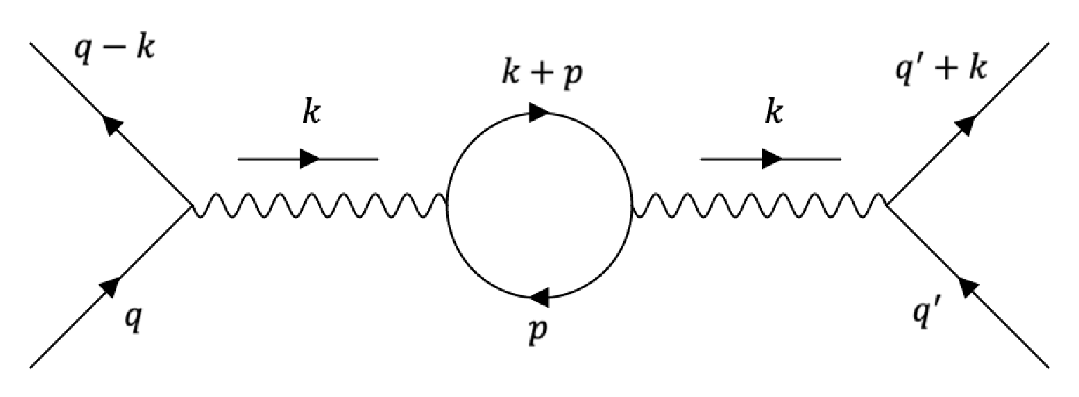
The calculations in Sections 3.1 and 3.2 pertain to ‘soft’ scattering processes in that they involve momentum transfers that are well below the electron mass scale. In this section we present a 1-loop calculation that involves momentum transfers that are considerably above the electron mass scale. Specifically, we calculate, at 1-loop, the running of the fine structure ‘constant’ at scales that are from one to four orders of magnitude above the electron mass threshold. The prediction of autoregularization, denoted αA​R(k)\alpha_{{}_{AR}}(k), agrees with the previously known result, derived using cutoff regularization scheme, denoted αC​R(k)\alpha_{{}_{CR}}(k), to within 0.8% as shown in Figure 4.

Consider the electron-electron scattering process 𝒫{\cal P}

𝒫:e−+e−→e−+e−\displaystyle{\cal P}:\qquad e^{-}+e^{-}\rightarrow\,e^{-}+e^{-}

shown in Figure 2. The 4-momentum transferred between the scattering electrons is denoted kk.

Refer to caption
Figure 2: Electron-electron scattering with 1-loop correction to photon propagator.

We consider scattering in which the incident electrons are nonrelativistic in the center-of-momentum frame ℱ{\cal F}, in which we work, but the transferred momentum kk has large invariant norm, |kμ​kμ|≫me\sqrt{|k^{\mu}k_{\mu}|}\gg m_{{}_{e}}. Thus, from (13), the intrinsic scale of the process is τ=|kμ​kμ|\tau\ =\ \sqrt{|k^{\mu}k_{\mu}|}.

The full photon propagator of the interacting photon field is (see Appendix D)

M~f​u​l​lμ​ν(k)\displaystyle\tilde{M}^{\mu\nu}_{{}_{full}}(k) =\displaystyle= M~μ​ν​(k)1−e2⋅gp2(k)⋅χ(k)\displaystyle\displaystyle\frac{\tilde{M}^{\mu\nu}(k)}{1-e^{2}\cdot g_{{}_{p}}^{2}(k)\cdot\chi(k)} (27)

where M~μ​ν​(k)\tilde{M}^{\mu\nu}(k) is the propagator of the free photon field, gp(k;ℱ,𝒫)g_{{}_{p}}(k;{\cal F},{\cal P}) is abbreviated to gp(k)g_{{}_{p}}(k) and

Πα​β(k)\displaystyle\Pi_{{}_{\alpha\beta}}(k) =\displaystyle= ie2(k2ηα​β−kαkβ)χ(k),χ(k):=Πμμ​(k)3​i​e2​k2\displaystyle i\,e^{2}\,(k^{2}\eta_{{}_{\alpha\beta}}-k_{\alpha}k_{\beta})\,\chi(k),\qquad\chi(k):=\displaystyle\frac{\Pi^{\mu}\,_{\mu}(k)}{3\,i\,e^{2}\,k^{2}} (28)

Following [2], we define a scale-dependent coupling as

e2​(k)\displaystyle e^{2}(k) :⁣=\displaystyle:= Z​e21−e2⋅gp2(k)⋅χ(k)\displaystyle\displaystyle\frac{Ze^{2}}{1-e^{2}\cdot g_{{}_{p}}^{2}(k)\cdot\chi(k)} (29)

where ee is the QED coupling constant that appears in the unrenormalized QED lagrangian, and ZZ is a constant. Since

limk→ 0gp2(k)χ(k)\displaystyle\lim_{k\rightarrow\,0}\ g_{{}_{p}}^{2}(k)\,\chi(k) =\displaystyle= 0\displaystyle 0

we can set Z=1Z=1 by imposing the boundary condition e2​(0)=e2=α/(4​π)e^{2}(0)=e^{2}=\sqrt{\alpha/(4\pi)}, where α\alpha is the fine structure constant. That is, we set the coupling constant ee in the QED lagrangian to be the scale-dependent coupling at zero momentum transfer, also called the ‘physical charge’ of an electron. Again, with some abuse of notation, we define 4​π​α​(k):=e2​(k)4\pi\alpha(k):=e^{2}(k). α⁡(k)\alpha(k) is the running fine structure constant. With some abuse of notation we have denoted α⁡(0)\alpha(0) as α\alpha. From (29) we have

α⁡(k)α\displaystyle\displaystyle\frac{\alpha(k)}{\alpha} =\displaystyle= 11−4παgp2(k)χ(k)= 1+4παgp2(k)χ(k)+O(e4)\displaystyle\displaystyle\frac{1}{1-4\pi\,\alpha\,g_{{}_{p}}^{2}(k)\,\chi(k)}\ =\ 1+4\pi\,\alpha\,g_{{}_{p}}^{2}(k)\,\chi(k)+O(e^{4}) (30)

The running of α⁡(k)\alpha(k) with kk at O⁡(α)O(\alpha), shown in (30), is a prediction of autoregularization. We compare the prediction (30) with previously known results below.

From Figure 2, at O⁡(α)O(\alpha) we have

Πμ​ν​(k)\displaystyle\Pi^{\mu\nu}(k) =\displaystyle= e2​∫d4​q(2​π)4​T​r​{γμ​D​(k+q)​γν​D​(q)},D⁡(q)=i⋅ge2(q)⋅(q/+me)q2−me2+iϵ\displaystyle e^{2}\int\displaystyle\frac{d^{4}q}{(2\pi)^{4}}\ \,Tr\left\{\gamma^{\mu}D(k+q)\gamma^{\nu}D(q)\right\},\hskip 18.49988ptD(q)\ =\ i\cdot\displaystyle\frac{g_{{}_{e}}^{2}(q)\cdot(q\!\!\!/+m_{{}_{e}})}{q^{2}-m_{{}_{e}}^{2}+i\epsilon}

where we have abbreviated ge(q;ℱ,𝒫)g_{{}_{e}}(q;{\cal F},{\cal P}) as ge(q)g_{{}_{e}}(q). Therefore,

Πμμ​(k)\displaystyle\Pi^{\mu}\,_{\mu}(k) =\displaystyle= e2​∫d4​q(2​π)4​ge2(k+q)⋅ge2(q)⋅[ 8(k+q)⋅q−16me2]((k+q)2−me2+iϵ)(q2−me2+iϵ)\displaystyle e^{2}\int\displaystyle\frac{d^{4}q}{(2\pi)^{4}}\ \displaystyle\frac{g_{{}_{e}}^{2}(k+q)\cdot g_{{}_{e}}^{2}(q)\cdot\left[\,8(k+q)\cdot q-16m_{{}_{e}}^{2}\,\right]}{((k+q)^{2}-m_{{}_{e}}^{2}+i\epsilon)(q^{2}-m_{{}_{e}}^{2}+i\epsilon)} (31)

The integral is calculated numerically. The q0q^{0} integral is calculated first using contour integration and the subsequent integration done using spherical coordinates. Substituting (31) into (28), we can evaluate χ⁡(k)\chi(k), and thus the ratio α⁡(k)/α\alpha(k)/\alpha shown in (30).

It is well-known [2, Equation 13.63] that for large, negative k2/me2k^{2}/m_{{}_{e}}^{2}, cutoff regularization scheme (CR) yields

α⁡(k)α\displaystyle\displaystyle\frac{\alpha(k)}{\alpha} =\displaystyle= 1+α3​π​ln⁡|k2|me2+O⁡(α2)\displaystyle 1+\displaystyle\frac{\alpha}{3\pi}\,\ln\displaystyle\frac{|k^{2}|}{m_{{}_{e}}^{2}}+O(\alpha^{2}) (32)

Denoting the α⁡(k)\alpha(k) in (32), obtained using cutoff regularization, as αC​R(k)\alpha_{{}_{CR}}(k) and the α⁡(k)\alpha(k) in (30), obtained using autoregularization, as αA​R(k)\alpha_{{}_{AR}}(k), at O(α\alpha), we obtain, using (30) and (32), the ratio

αA​R(k)αC​R(k)\displaystyle\displaystyle\frac{\alpha_{{}_{AR}}(k)}{\alpha_{{}_{CR}}(k)} =\displaystyle= 1+4παge2(k)⋅χ(k)1+α3​π​ln⁡|k2|me2, at ​O​(α)\displaystyle\displaystyle\frac{1+4\pi\,\alpha\,g_{{}_{e}}^{2}(k)\cdot\chi(k)}{1+\displaystyle\frac{\alpha}{3\pi}\,\ln\displaystyle\frac{|k^{2}|}{m_{{}_{e}}^{2}}},\qquad\mbox{ at }O(\alpha) (33)

Refer to caption

Figure 3: Growth of αA​R\alpha_{{}_{AR}} with −k2/me\sqrt{-k^{2}}/m_{{}_{e}} over the range 10⩽−k2/me⩽10410\leq\sqrt{-k^{2}}/m_{{}_{e}}\leq 10^{4}, and for kμ​𝒰μ​(ℱ,ℱ)=200,400,600,800k_{\mu}{\cal U}^{\mu}({\cal F};{\cal F})=200,400,600,800 and 10001000. The inset shows the plot for 10⩽−k2/me⩽10310\leq\sqrt{-k^{2}}/m_{{}_{e}}\leq 10^{3}.

Figure 3 shows the plot of αA​R​(k)/α\alpha_{AR}(k)/\alpha, for 10⩽−k2/me⩽10410\leq\sqrt{-k^{2}}/m_{{}_{e}}\leq 10^{4}. The graphs confirm that the QED coupling constant αA​R(k)\alpha_{{}_{AR}}(k), predicted by autoregularization, increases with invariant momentum transfer −k2\sqrt{-k^{2}}, as expected [2]. Figure 4 provides a comparison with the previously known results. The plot of αA​R​(k)/αC​R​(k)\alpha_{AR}(k)/\alpha_{CR}(k) shows that the discrepancy between αA​R​(k)\alpha_{AR}(k), and αC​R​(k)\alpha_{CR}(k) is less than 0.8% over the above range of −k2/me\rule{0.0pt}{11.0pt}\sqrt{-k^{2}}/m_{{}_{e}} and less than 0.5% at momentum transfer scale of 104me{}^{4}\,m_{{}_{e}}.

[Uncaptioned image]

Figure 4: Comparison of the prediction of autoregularization (αA​R\alpha_{{}_{AR}}) with the prediction of cutoff regularization (αC​R\alpha_{{}_{CR}}), for 10⩽−k2/me⩽10410\leq\sqrt{-k^{2}}/m_{{}_{e}}\leq 10^{4} and kμ​𝒰μ​(ℱ,ℱ)=200,400,600,800k_{\mu}{\cal U}^{\mu}({\cal F};{\cal F})=200,400,600,800 and 10001000. The inset shows the plot for 10⩽−k2/me⩽10310\leq\sqrt{-k^{2}}/m_{{}_{e}}\leq 10^{3}.

3.4 Asymptotic freedom in QCD

We compute the running of the QCD coupling constant at 1-loop and show that autoregularization, like other known regularization schemes, also predicts the well-known asymptotic freedom in QCD.

The lagrangian of the QCD sector, denoted ℒQ​C​D{\cal L}_{QCD}, is

ℒQ​C​D\displaystyle{\cal L}_{QCD} :⁣=\displaystyle:= q¯cf(i∂−gG/a(Ta)c​d−mf)qdf−14Gμ​νaGa−μ​ν12​ξ(∂μGμa)2+∂μω†Dμaωa\displaystyle\bar{q}^{f}_{c}\left(i\cancel{\partial}-gG\!\!\!\!/^{a}(T^{a})_{cd}-m_{f}\right)q^{f}_{d}-\frac{1}{4}G_{\mu\nu}^{a}G^{a}\,{}^{\mu\nu}-\displaystyle\frac{1}{2\xi}\left(\partial^{\mu}G_{\mu}^{a}\right)^{2}+\partial^{\mu}\omega^{\dagger}\ {}^{a}D_{\mu}\omega^{a}
Gμ​νa\displaystyle G_{\mu\nu}^{a} :⁣=\displaystyle:= ∂μGνa−∂νGμa−g​fa​r​s​Gμr​Gνs\displaystyle\partial_{\mu}G_{\nu}^{a}-\partial_{\nu}G_{\mu}^{a}-gf^{ars}G_{\mu}^{r}G_{\nu}^{s}
Dμ​ωa\displaystyle D_{\mu}\omega^{a} :⁣=\displaystyle:= ∂μωa−g​fa​r​s​ωr​Gμs\displaystyle\partial_{\mu}\omega^{a}-gf^{ars}\omega^{r}G_{\mu}^{s} (34)

where q,G,ω,ω†q,G,\omega,\omega^{\dagger} denote the quark, gluon, ghost and antighost fields respectively. The sum over repeated flavor index ff (quark flavors), the color indices c,dc,d and group indices a,r,sa,r,s is implied. Ta=λa/2T^{a}=\lambda^{a}/2 are the generators of S​U​(3)SU(3) where λa\lambda^{a} are the Gellmann matrices. fa​r​sf^{ars} are the structure constants of S​U​(3)SU(3) and gg the QCD coupling constant.

At O⁡(g2)O(g^{2}) the gluon propagator receives corrections from the four loops shown in Figure 5. The quark loop is shown in solid line, the ghost loop in dashed line and the gluon loops in curly lines. The gluon loops at O⁡(g2)O(g^{2}) arise from 3-gluon and 4-gluon self-interaction terms in ℒQ​C​D{\cal L}_{QCD}. The labels represent momenta.

The full gluon propagator can be written as

Kμ​ν​(x−y)\displaystyle K^{\mu\nu}(x-y) =\displaystyle= ∫d4​k(2​π)4​e−i​k​(x−y)​K~μ​ν​(k)\displaystyle\int\displaystyle\frac{d^{4}k}{(2\pi)^{4}}\ e^{\displaystyle-ik(x-y)}\tilde{K}^{\mu\nu}(k)
K~μ​ν​(k)\displaystyle\tilde{K}^{\mu\nu}(k) =\displaystyle= K~0μα1(k)∑n=1∞Σα1β1(k)K~0β1α2(k)…Σαnβn(k)K~0βnν(k),K~0α​β(k)=−i​ημ​ν​gg2​(k)k2+i​ϵ\displaystyle\tilde{K}_{{}_{0}}^{\mu\alpha_{{}_{1}}}(k)\,\sum_{n=1}^{\infty}\Sigma_{{}_{\alpha_{{}_{1}}\beta_{{}_{1}}}}(k)\tilde{K}_{{}_{0}}^{\beta_{{}_{1}}\alpha_{{}_{2}}}(k)\,\ldots\Sigma_{{}_{\alpha_{{}_{n}}\beta_{{}_{n}}}}(k)\tilde{K}_{{}_{0}}^{\beta_{{}_{n}}\nu}(k),\hskip 9.24994pt\tilde{K}^{\alpha\beta}_{{}_{0}}(k)\ =\ \displaystyle\frac{-i\eta^{\mu\nu}\,g^{2}_{g}(k)}{k^{2}+i\epsilon}

where ggg_{g} denotes the Gibbs factor1414 14 We consider the gluon propagator for a q+q→q+qq+q\rightarrow\,q+q scattering process and work in the center-of-momentum frame of the scattering process. of the gluon and K~0\tilde{K}_{{}_{0}} the propagator1515 15 As we show below, kμ​Σμ​ν​(k)=Σμ​ν​(k)​kν= 0k^{\mu}\Sigma_{\mu\nu}(k)\ =\ \Sigma_{\mu\nu}(k)k^{\nu}\ =\ 0. of the free gluon. As with the photon propagator we use the ansatz that

Σα​β​(k)\displaystyle\Sigma_{\alpha\beta}(k) =\displaystyle= ig2(gα​βk2−kαkβ)χg(k),χg(k)=Σαα​(k)3​i​g2​k2\displaystyle ig^{2}(g_{\alpha\beta}k^{2}-k_{\alpha}k_{\beta})\chi_{{}_{g}}(k),\qquad\chi_{{}_{g}}(k)\ =\ \displaystyle\frac{\Sigma^{\alpha}_{\alpha}(k)}{3\,i\,g^{2}\,k^{2}}\ (35)

The ansatz implies

kα​Σα​β​(k)\displaystyle k^{\alpha}\Sigma_{\alpha\beta}(k) =\displaystyle= 0\displaystyle 0 (36)

For the photon propagator kα​Πα​β​(k)= 0k^{\alpha}\Pi_{\alpha\beta}(k)\ =\ 0 followed from current conservation at the vertex to which the photon line attaches. On the other hand, the gluon line attaches to four types of vertices, as shown in Figure 5. In order to use the ansatz (35), therefore, we need to establish the transversality condition (36) for all the four diagrams in Figure 5.

[Uncaptioned image][Uncaptioned image][Uncaptioned image][Uncaptioned image]

Figure 5: 1-loop corrections to the gluon propagator. The quark loop (left) and ghost loop (right) are shown above and the gluon loops below.

Consider the quark loop at O⁡(g2)O(g^{2}) shown in Figure 5.

I(q)(a​b)(x−y)α​β\displaystyle I_{(q)}^{(ab)}\,{}^{\alpha\beta}(x-y) =\displaystyle= 12!⟨0∣T(Ga)α(x)[−ig∫(Gr)μ(w)Jμr(w)dw]\displaystyle\displaystyle\frac{1}{2!}\langle 0\mid T(G^{a})^{\alpha}(x)\left[\,-ig\int(G^{r})^{\mu}(w)J^{r}_{\mu}(w)\,dw\,\right]
[−ig∫(Gs)ν(z)Jνs(z)dz](Gb)β(y)∣0⟩\displaystyle\hskip 86.72377pt\left[\,-ig\int(G^{s})^{\nu}(z)J^{s}_{\nu}(z)\,dz\,\right](G^{b})^{\beta}(y)\mid 0\rangle
=\displaystyle= −g2∫d4​k(2​π)4e−i​k​(x−y)δa​bK~0α​μ(k)Σμ​ν(q)(k)K~0ν​β(k)\displaystyle-g^{2}\int\displaystyle\frac{d^{4}k}{(2\pi)^{4}}\ e^{\displaystyle-ik(x-y)}\delta^{ab}\ \tilde{K}^{\alpha\mu}_{{}_{0}}(k)\ \Sigma^{(q)}_{\mu\nu}(k)\ \tilde{K}^{\nu\beta}_{{}_{0}}(k)

where

Jμr​(w)\displaystyle J^{r}_{\mu}(w) =\displaystyle= [q¯cf​γμ​qdf]​Tc​dr\displaystyle\left[\,\bar{q}^{f}_{c}\gamma_{\mu}q^{f}_{d}\,\right]T^{r}_{cd}

Since qcfq^{f}_{c} and qdfq^{f}_{d} have the same mass,

∂μJμr\displaystyle\partial^{\mu}J^{r}_{\mu} =\displaystyle= 0\displaystyle 0 (37)

Owing to the current conservation (37), kμ​Σμ​ν(q)​(k)= 0k^{\mu}\Sigma_{\mu\nu}^{(q)}(k)\ =\ 0.

Next, consider the ghost loop. The ghost lagrangian is

ℒg​h=∂μω†Dμaωa=∂μ{ω†Dμaωa}−ω†∂μaDμωa≡−ω†∂μaDμωa\displaystyle{\cal L}_{gh}\ =\ \partial^{\mu}\omega^{\dagger}\ {}^{{}^{a}}D_{\mu}\omega^{a}\ =\ \partial^{\mu}\left\{\omega^{\dagger}\ {}^{{}^{a}}D_{\mu}\omega^{a}\right\}-\omega^{\dagger}\ {}^{{}^{a}}\partial^{\mu}D_{\mu}\omega^{a}\equiv-\omega^{\dagger}\ {}^{{}^{a}}\partial^{\mu}D_{\mu}\omega^{a}

where we have disregarded the divergence term. Hence the ghost lagrangian can be written equivalently as

ℒg​h\displaystyle{\cal L}_{gh} =\displaystyle= 12{∂μω†Dμaωa−ω†∂μaDμωa}\displaystyle\frac{1}{2}\left\{\partial^{\mu}\omega^{\dagger}\ {}^{{}^{a}}D_{\mu}\omega^{a}-\omega^{\dagger}\ {}^{{}^{a}}\partial^{\mu}D_{\mu}\omega^{a}\right\}

The ghost-gluon interaction term in the lagrangian is

Vg​h\displaystyle V_{gh} =\displaystyle= −gfa​b​c(∂μω†)aωb(Gc)μ+gfa​b​cω†(∂μωb)a(Gc)μ+gfa​b​cω†ωba∂μ(Gc)μ\displaystyle-gf^{abc}\left(\partial^{\mu}\omega^{\dagger}\ {}^{{}^{a}}\right)\omega^{b}(G^{c})_{\mu}+gf^{abc}\omega^{\dagger}\ {}^{{}^{a}}\left(\partial^{\mu}\omega^{b}\right)(G^{c})_{\mu}+gf^{abc}\omega^{\dagger}\ {}^{{}^{a}}\omega^{b}\partial^{\mu}(G^{c})_{\mu}

The third term vanishes due to Lorenz gauge condition ∂μ(Gc)μ= 0\partial^{\mu}(G^{c})_{\mu}\ =\ 0. Therefore

Vg​h\displaystyle V_{gh} =\displaystyle= gfa​b​c(−(∂μω†a)ωb+ω†a∂μωb)⏟Jμa​b(Gc)μ\displaystyle gf^{abc}\underbrace{\left(-(\partial^{\mu}\omega^{\dagger}\ {}^{{}^{a}})\omega^{b}+\omega^{\dagger}\ {}^{{}^{a}}\partial^{\mu}\omega^{b}\right)}_{J^{\mu}\,{}^{ab}}(G^{c})_{\mu}

Note that

∂μJμa​b\displaystyle\partial_{\mu}J^{\mu}\,{}^{ab} =\displaystyle= −(□ω†)aωb+ω†□aωb= 0\displaystyle-\left(\Box\,\omega^{\dagger}\ {}^{{}^{a}}\right)\omega^{b}+\omega^{\dagger}\ {}^{{}^{a}}\Box\,\omega^{b}\ =\ 0 (38)

since □ω†a=□ωb= 0\Box\,\omega^{\dagger}\ {}^{{}^{a}}\ =\ \Box\,\omega^{b}\ =\ 0 for fields ω†a\omega^{\dagger}\ {}^{{}^{a}} and ωb\omega^{b} in the interaction picture. The current conservation (38) implies that kμ​Σα​β(g​h)​(k)= 0k^{\mu}\Sigma_{\alpha\beta}^{(gh)}(k)\ =\ 0, establishing the transversality condition for the ghost loop.

The O⁡(g2)O(g^{2}) correction due to the gluon loop containing 3-gluon vertices (bottom left in Figure 5) is1616 16 since fr​q​s​(∂μ(Gr)ν−∂ν(Gr)μ)​(Gq)μ​(Gs)ν= 2​fr​q​s​∂μ(Gr)ν​(Gq)μ​(Gs)νf^{rqs}(\partial_{\mu}(G^{r})_{\nu}-\partial_{\nu}(G^{r})_{\mu})(G^{q})^{\mu}(G^{s})^{\nu}\ =\ 2f^{rqs}\partial_{\mu}(G^{r})_{\nu}(G^{q})^{\mu}(G^{s})^{\nu}

I3​ga​b(x−y)α​β\displaystyle I^{ab}_{3g}\,{}^{\alpha\beta}(x-y) =\displaystyle= g2fj​k​lfe​r​s∫d4w∫d4z[−δa​j(K0)α​μ(x−w)\displaystyle g^{2}f^{jkl}f^{ers}\int d^{4}w\int d^{4}z\,\left[-\delta^{aj}\left(K_{{}_{0}}\right)^{\alpha\mu}(x-w)\right.
⟨ 0​|T​[∂λ((Gk)λ​(Gl)μ)]w​[∂ρ(Ge)σ​(Gr)ρ​(Gs)σ]z​(Gb)β​(y)|​0⟩c\displaystyle\left\langle\,0\left|\,T\left[\,\partial_{\lambda}\left((G^{k})^{\lambda}(G^{l})_{\mu}\right)\,\right]_{w}\left[\,\partial_{\rho}(G^{e})_{\sigma}(G^{r})^{\rho}(G^{s})^{\sigma}\,\right]_{z}(G^{b})^{\beta}(y)\,\right|0\,\right\rangle_{c}
+δa​k(K0)α​μ(x−w)⟨ 0|T[∂μ(Gj)λ(Gl)λ]w[∂ρ(Ge)σ(Gr)ρ(Gs)σ]z(Gb)β(y)|0⟩c\displaystyle+\delta^{ak}\,(K_{{}_{0}})^{\alpha\mu}(x-w)\left\langle\,0\left|\,T\left[\,\partial_{\mu}(G^{j})_{\lambda}(G^{l})^{\lambda}\,\right]_{w}\left[\,\partial_{\rho}(G^{e})_{\sigma}(G^{r})^{\rho}(G^{s})^{\sigma}\,\right]_{z}(G^{b})^{\beta}(y)\,\right|0\,\right\rangle_{c}
+δa​l(K0)α​μ(x−w)⟨ 0|T[∂λ(Gj)μ(Gk)λ]w[∂ρ(Ge)σ(Gr)ρ(Gs)σ]z(Gb)β(y)|0⟩c]\displaystyle\left.+\delta^{al}\,(K_{{}_{0}})^{\alpha\mu}(x-w)\left\langle\,0\left|\,T\left[\,\partial_{\lambda}(G^{j})_{\mu}(G^{k})^{\lambda}\,\right]_{w}\left[\,\partial_{\rho}(G^{e})_{\sigma}(G^{r})^{\rho}(G^{s})^{\sigma}\,\right]_{z}(G^{b})^{\beta}(y)\,\right|0\,\right\rangle_{c}\right]
=\displaystyle= g2fj​k​lfe​r​sδa​b∫d4​k(2​π)4e−i​k​(x−y)K~0α​μ(k)Σμ​ν(3​g)(k)K~0ν​β(k)\displaystyle g^{2}\,f^{jkl}\,f^{ers}\ \delta^{ab}\,\int\displaystyle\frac{d^{4}k}{(2\pi)^{4}}\ e^{\displaystyle-ik(x-y)}\tilde{K}_{{}_{0}}^{\alpha\mu}(k)\ \Sigma^{(3g)}_{\mu\nu}(k)\ \tilde{K}_{{}_{0}}^{\nu\beta}(k)

where ⟨ 0​|T​…|​0⟩c\left\langle\,0\left|\,T\ldots\,\right|0\,\right\rangle_{c} denotes the connected diagram, in which the GG fields at one vertex Wick-contract necessarily with the GG fields at the other vertex.

In order to show that kμΣμ​ν(3​g)(k)= 0k^{\mu}\Sigma^{(3g)}_{{}_{\mu\nu}}(k)\ =\ 0, it is sufficient to show that

fj​k​lfe​r​s∂μ[−∂λ((Gk)λ(Gl)μ)δa​j+δa​k∂μ(Gj)λ(Gk)λ+δa​l∂λ(Gj)μ(Gk)λ]\displaystyle f^{jkl}f^{ers}\partial^{\mu}\left[\,-\partial_{\lambda}\left((G^{k})^{\lambda}(G^{l})_{\mu}\right)\delta^{aj}+\delta^{ak}\partial_{\mu}(G^{j})_{\lambda}(G^{k})^{\lambda}+\delta^{al}\partial_{\lambda}(G^{j})_{\mu}(G^{k})^{\lambda}\,\right] =\displaystyle= 0\displaystyle 0 (39)

The first term in (39) vanishes due to Lorenz gauge condition ∂μ(G(.))μ= 0\partial^{\mu}(G^{(.)})_{\mu}\ =\ 0. The second term vanishes since □​(Gj)λ= 0\Box(G^{j})_{\lambda}\ =\ 0 in the interaction picture and fj​k​lf^{jkl} is totally antisymmetric. The third term vanishes due to Lorenz gauge condition and the antisymmetry of fj​k​lf^{jkl}.

Finally, consider the gluon loop comprising the 4-gluon interaction vertex.

I4​ga​b(x−y)α​β\displaystyle I_{4g}^{ab}\,{}^{\alpha\beta}(x-y) =\displaystyle= −ig2∫fa​j​kfa​r​sd4z⟨ 0|T(Ga)α(x)[(Gj)μ(Gk)ν(Gr)μ(Gs)ν]z(Gb)β(y)|0⟩\displaystyle-ig^{2}\int f^{ajk}f^{ars}d^{4}z\,\left\langle\,0\left|\,T(G^{a})^{\alpha}(x)\left[\,(G^{j})_{\mu}(G^{k})_{\nu}(G^{r})^{\mu}(G^{s})^{\nu}\,\right]_{z}(G^{b})^{\beta}(y)\,\right|0\,\right\rangle
=\displaystyle= −ig2δa​b∫d4​k(2​π)4e−i​k​(x−y)K~0α​μ(k)Σμ​ν(4​g)(k)K~0ν​β(k)\displaystyle-ig^{2}\,\delta^{ab}\int\displaystyle\frac{d^{4}k}{(2\pi)^{4}}\ e^{\displaystyle-ik(x-y)}\tilde{K}_{{}_{0}}^{\alpha\mu}(k)\ \Sigma^{(4g)}_{{}_{\mu\nu}}(k)\ \tilde{K}_{{}_{0}}^{\nu\beta}(k)

We note that two of the four gluon fields (Gj)μ,(Gk)ν,(Gr)μ,(Gs)ν(G^{j})_{\mu},\,(G^{k})_{\nu},\,(G^{r})^{\mu},\,(G^{s})^{\nu} Wick-contract to form the loop shown (at the bottom right) in Figure 5 leaving two terms of the form (Gu)λ​(Gv)λ(G^{u})_{\lambda}(G^{v})^{\lambda} that Wick-contract with (Ga)α(G^{a})^{\alpha} and (Gb)β(G^{b})^{\beta}. Further, due to the antisymmetry of fa​j​kf^{ajk} and fa​r​sf^{ars}, uu and vv cannot both belong to either {j,k}\left\{j,k\right\} or {r,s}\left\{r,s\right\}.

Without loss of generality assume that (Ga)α(G^{a})^{\alpha} Wick-contracts with (Gr)μ(G^{r})^{\mu}. Then to show that kμ​Σμ​ν(4​g)​(k)= 0k^{\mu}\Sigma^{(4g)}_{\mu\nu}(k)\ =\ 0 it suffices to show that

∂μ[(Gj)μ​(Gk)ν​(Gs)ν﹈+(Gk)ν​(Gj)μ​(Gs)ν﹈]\displaystyle\partial^{\mu}\left[\,(G^{j})_{\mu}\underbracket{(G^{k})_{\nu}(G^{s})^{\nu}}+(G^{k})_{\nu}\underbracket{(G^{j})_{\mu}(G^{s})^{\nu}}\,\right] =\displaystyle= 0\displaystyle 0

where A​B﹈\underbracket{AB} represents Wick-contraction. The first term vanishes due to Lorenz gauge condition. The Wick-contraction in the second term makes the remaining term (Gk)μ(G^{k})_{\mu} and hence the second term also vanishes due to Lorenz gauge condition.

The above argument shows that

kμ​Σμ​ν​(k)\displaystyle k^{\mu}\Sigma_{\mu\nu}(k) =\displaystyle= 0\displaystyle 0

where

Σμ​ν​(k):=Σμ​ν(q)​(k)+Σμ​ν(g​h)​(k)+Σμ​ν(3​g)​(k)+Σμ​ν(4​g)​(k)\displaystyle\Sigma_{\mu\nu}(k):=\Sigma_{\mu\nu}^{(q)}(k)+\Sigma_{\mu\nu}^{(gh)}(k)+\Sigma_{\mu\nu}^{(3g)}(k)+\Sigma_{\mu\nu}^{(4g)}(k) (40)

The argument can be adapted to also show that

kν​Σμ​ν​(k)\displaystyle k^{\nu}\Sigma_{\mu\nu}(k) =\displaystyle= 0\displaystyle 0

Once again, defining

Pμ​ν​(k)\displaystyle P_{\mu\nu}(k) :⁣=\displaystyle:= ημ​ν−kμ​kνk2\displaystyle\eta_{\mu\nu}-\displaystyle\frac{k_{\mu}k_{\nu}}{k^{2}}

and noting Pαμ​(k)​Pνα​(k)=Pνμ​(k)P^{\mu}_{\alpha}(k)P^{\alpha}_{\nu}(k)\ =\ P^{\mu}_{\nu}(k) we see that

Σα1β1(k)K~0β1α2(k)…Σαn−1​βn−1(k)K~0βn−1αn(k)\displaystyle\Sigma_{\alpha_{{}_{1}}\beta_{{}_{1}}}(k)\tilde{K}_{{}_{0}}^{\beta_{{}_{1}}\alpha_{{}_{2}}}(k)\ldots\Sigma_{\alpha_{n-1}\beta_{n-1}}(k)\tilde{K}_{{}_{0}}^{\beta_{n-1}\alpha_{{}_{n}}}(k) =\displaystyle= λn−1Pα1αn(k),λ=g2gg2(k)χg(k)\displaystyle\lambda^{n-1}P^{\alpha_{{}_{n}}}_{\alpha_{{}_{1}}}(k),\qquad\lambda\ =\ g^{2}\,g_{g}^{2}(k)\,\chi_{g}(k)

Therefore,

K~μ​ν​(k)\displaystyle\tilde{K}^{\mu\nu}(k) =\displaystyle= K~0μ​ν(k)+K~0μ​α(k)[∑n=1∞λn]Pαν(k)=K~0μ​ν(k)+K~0μ​ν(k)[λ1−λ]Pαν(k)\displaystyle\tilde{K}_{{}_{0}}^{\mu\nu}(k)+\tilde{K}_{{}_{0}}^{\mu\alpha}(k)\left[\,\sum_{n=1}^{\infty}\lambda^{n}\,\right]P^{\nu}_{\alpha}(k)\ =\ \tilde{K}_{{}_{0}}^{\mu\nu}(k)+\tilde{K}_{{}_{0}}^{\mu\nu}(k)\left[\,\frac{\lambda}{1-\lambda}\,\right]P^{\nu}_{\alpha}(k)
:⁣=\displaystyle:= K~0μ​ν(k)+K~0μ​ν(k)[g~2(k)gg2(k)χg(k)]Pαν(k)\displaystyle\tilde{K}_{{}_{0}}^{\mu\nu}(k)+\tilde{K}_{{}_{0}}^{\mu\nu}(k)\left[\,\tilde{g}^{2}(k)g_{g}^{2}(k)\chi_{g}(k)\,\right]P^{\nu}_{\alpha}(k)

where the scale-dependent coupling constant is

g~2​(k)\displaystyle\tilde{g}^{2}(k) :⁣=\displaystyle:= g21−g2​gg2​(k)​χg​(k)\displaystyle\displaystyle\frac{g^{2}}{1-g^{2}g_{g}^{2}(k)\chi_{g}(k)}

Since gg2​χg​(k)→ 0g_{g}^{2}\chi_{g}(k)\rightarrow\,0 as k→ 0k\rightarrow\,0, g=g~​(0)g\ =\ \tilde{g}(0). Defining αQ​C​D(k):=4πg~2(k)\alpha_{{}_{QCD}}(k):=4\pi\tilde{g}^{2}(k) to be the QCD coupling constant at momentum kk, we obtain

αQ​C​D(k)\displaystyle\alpha_{{}_{QCD}}(k) =\displaystyle= αQ​C​D(0)1−4παQ​C​D(0)gg2(k)χg(k),\displaystyle\displaystyle\frac{\alpha_{{}_{QCD}}(0)}{1-4\pi\alpha_{{}_{QCD}}(0)\,g_{g}^{2}(k)\chi_{g}(k)}, (41)

If χg(k)<0\chi_{{}_{g}}(k)<0 and |gg2(k)χg(k)||g_{{}_{g}}^{2}(k)\chi_{{}_{g}}(k)| increases as −k2-k^{2} increases then the QCD coupling constant αQ​C​D(k)\alpha_{{}_{QCD}}(k) decreases with the gluon propagator scale −k2\sqrt{-k^{2}}, signaling asymptotic freedom.

From (35) and (40), the calculation of χg​(k)\chi_{g}(k) reduces to the calculation of Σα​β(q)​(k),Σα​β(g​h)​(k),\Sigma_{\alpha\beta}^{(q)}(k),\Sigma_{\alpha\beta}^{(gh)}(k), Σα​β(3​g)​(k)\Sigma_{\alpha\beta}^{(3g)}(k) and Σα​β(4​g)​(k)\Sigma_{\alpha\beta}^{(4g)}(k). A lengthy calculation using ℒQ​C​D{\cal L}_{{}_{QCD}} in (34) yields

(Σ(q))αα\displaystyle(\Sigma^{(q)})^{\alpha}_{\alpha} =\displaystyle= (12)​g2​∑f∫d4​p(2​π)4​T​r​{γα​Q~f​(k+p)​γα​Q~f​(p)},Q~f​(p):=i​(gqf​(k))2k/−mf+iϵ\displaystyle\left(\frac{1}{2}\right)g^{2}\sum_{f}\int\displaystyle\frac{d^{4}p}{(2\pi)^{4}}\ Tr\left\{\gamma^{\alpha}\tilde{Q}^{f}(k+p)\gamma_{\alpha}\tilde{Q}^{f}(p)\right\},\hskip 50.58878pt\tilde{Q}^{f}(p):=\displaystyle\frac{i(g_{q}^{f}(k))^{2}}{k\!\!\!/-m^{f}+i\epsilon}
(Σ(g​h))αα\displaystyle(\Sigma^{(gh)})^{\alpha}_{\alpha} =\displaystyle= 3​g2​∫d4​p(2​π)4​pα​(k+p)α​H~​(k+p)​H~​(p),H~​(p):=i​gg​h2​(p)p2+i​ϵ\displaystyle 3\,g^{2}\int\displaystyle\frac{d^{4}p}{(2\pi)^{4}}\ p^{\alpha}(k+p)_{\alpha}\tilde{H}(k+p)\tilde{H}(p),\hskip 101.17755pt\tilde{H}(p):=\displaystyle\frac{ig_{gh}^{2}(p)}{p^{2}+i\epsilon}
(Σ(3​g))αα\displaystyle(\Sigma^{(3g)})^{\alpha}_{\alpha} =\displaystyle= −3g2∫d4​p(2​π)4G~(p)G~(k−p)[ 12kαkα+9pαpα−15kαpα],G~(p):=−i​gg2​(p)p2+i​ϵ\displaystyle-3g^{2}\int\displaystyle\frac{d^{4}p}{(2\pi)^{4}}\ \tilde{G}(p)\tilde{G}(k-p)\left[\,12k^{\alpha}k_{\alpha}+9p^{\alpha}p_{\alpha}-15k^{\alpha}p_{\alpha}\,\right],\hskip 14.45377pt\tilde{G}(p):=\displaystyle\frac{-i\,g_{g}^{2}(p)}{p^{2}+i\epsilon}
(Σ(4​g))αα\displaystyle(\Sigma^{(4g)})^{\alpha}_{\alpha} =\displaystyle= −36ig2∫d4​p(2​π)4G~(p)\displaystyle-36\,i\,g^{2}\int\displaystyle\frac{d^{4}p}{(2\pi)^{4}}\ \tilde{G}(p) (42)
[Uncaptioned image]

Figure 6: Scattering of two quarks through gluon exchange. The labels represent 4-momenta. The figure shows only one of the possible gluon loops.

Consider a scattering process 𝒫{\cal P} in which two quarks scatter through a gluon exchange. Since we seek to study the variation of αQ​C​D(k)\alpha_{{}_{QCD}}(k) with increasing −k2-k^{2}, we assume that the momentum transfer scale −k2\sqrt{-k^{2}} is the dominant scale of the scattering process and hence τ𝒫=−k2\tau_{{}_{{\cal P}}}\ =\ \sqrt{-k^{2}}. The Gibbs factors of gluons and ghosts are given by the expressions for the Gibbs factors of massless bosons1717 17 Although ghosts and antighosts are strange in that they are described by Grassmann fields., both with two degrees of freedom (dφ= 2d_{{}_{\varphi}}\ =\ 2 in (2.2)). Numerical calculation yields the following plot for αQ​C​D(k)/αQ(0)\alpha_{{}_{QCD}}(k)/\alpha_{{}_{Q}}(0), confirming that the QCD coupling constant αQ​C​D(k)\alpha_{{}_{QCD}}(k) does decrease with increasing −k2\sqrt{-k^{2}} as shown. Thus autoregularization, like other known regularization schemes, also predicts the asymptotic freedom in QCD.

[Uncaptioned image]

Figure 7: Running of the QCD coupling constant αQ​C​D(k)\alpha_{{}_{QCD}}(k) with −k2\sqrt{-k^{2}}.

3.5 Scattering cross sections at tree-level

In the following subsections we use autoregularization to calculate the tree-level cross sections of two processes—Compton scattering and e+e^{+}-e−e^{-} pair annihilation—and compare the theoretical calculations with experimental data. While the energy scale of the experimental data for Compton scattering is ∼\sim MeV, the center-of-momentum energy of the pair annihilation experiment is ≳206\gtrsim 206 GeV. For both processes, the predictions of autoregularization are found to be in good agreement with experimental data.

3.5.1 Compton scattering

In the following discussion we compare a tree-level prediction of autoregularization with experimental data. Specifically, we calculate the angular distribution of the differential cross section for Compton scattering at tree level using autoregularization and compare the prediction with that of the well-known Klein-Nishina formula [37] as well as the experimental measurements of Friedrich and Goldhaber [10]. We perform the calculation in the laboratory frame.

In Compton scattering

𝒫:γ+e−→γ+e−\displaystyle{\cal P}:\quad\gamma+e^{-}\rightarrow\,\gamma+e^{-} (43)

incoming photon and electron scatter to outgoing photon and electron as shown in Figure 8.

Refer to caption
Figure 8: The kinematics of Compton scattering.

We assume the scattering occurs in the y−zy-z plane in the laboratory frame. An incoming photon of energy Eγ=ω1mec2=ω1E_{\gamma}=\omega_{{}_{1}}m_{{}_{e}}c^{2}=\omega_{{}_{1}} ( me=c=1m_{{}_{e}}=c=1 in natural units) collides with an electron, which is initially at rest in the laboratory frame, and scatters to an outgoing photon of energy Eγ′=ω2mec2=ω2E_{\gamma}^{\prime}=\omega_{{}_{2}}m_{{}_{e}}c^{2}=\omega_{{}_{2}} at an angle θ\theta relative to the zz-axis. The 4-momentum of the outgoing electron in laboratory frame is denoted q2q_{{}_{2}}.

Momentum conservation and the requirement that the outgoing electron is on mass shell determines ω2\omega_{{}_{2}} given ω1\omega_{{}_{1}} and θ\theta. Specifically, ω2\omega_{{}_{2}} is given by

ω2\displaystyle\omega_{{}_{2}} =\displaystyle= meω1me+ω1(1−cos(θ))\displaystyle\displaystyle\frac{m_{{}_{e}}\omega_{{}_{1}}}{m_{{}_{e}}+\omega_{{}_{1}}(1-\cos(\theta))} (44)

We choose ϵ(k1,1)=(0,1,0,0)\epsilon(k_{{}_{1}},1)=(0,1,0,0) and ϵ(k1,2)=(0,0,1,0)\epsilon(k_{{}_{1}},2)=(0,0,1,0) to be the basis transverse polarizations corresponding to the incoming photon and ϵ(k2,1)=(0,1,0,0)\epsilon(k_{{}_{2}},1)=(0,1,0,0) and ϵ(k2,2)=(0,0,cos(θ),−sin(θ))\epsilon(k_{{}_{2}},2)=(0,0,\cos(\theta),-\sin(\theta)) to be the basis transverse polarizations corresponding to the outgoing photon. We label the polarizations of the incoming and outgoing photons, ϵ(k1,r1)\epsilon(k_{{}_{1}},r_{{}_{1}}) and ϵ(k2,r2)\epsilon(k_{{}_{2}},r_{{}_{2}}) respectively, with r1,r2=1,2r_{{}_{1}},r_{{}_{2}}=1,2.

Refer to caption
Figure 9: The Feynman diagrams that contribute to the tree-level amplitude of Compton scattering.

At the tree level the scattering amplitude with incoming photon (electron) polarization1818 18 With slight abuse of notation we use the term polarization to denote the helicity of an electron. labeled r1r_{{}_{1}} (s1s_{{}_{1}}) and outgoing photon (electron) polarization r2r_{{}_{2}} (s2s_{{}_{2}}), denoted 𝒜2{\cal A}_{{}_{2}}, receives contributions from the two Feynman diagrams shown in Figure 9, and is given by

𝒜2({k1,r1},{q1,s1};{k2,r2},{q2,s2})\displaystyle{\cal A}_{{}_{2}}(\left\{k_{{}_{1}},r_{{}_{1}}\right\},\left\{q_{{}_{1}},s_{{}_{1}}\right\};\left\{k_{{}_{2}},r_{{}_{2}}\right\},\left\{q_{{}_{2}},s_{{}_{2}}\right\}) =\displaystyle= −i(2π)4δ4(q2+k2−q1−k1)ℳ2\displaystyle-i(2\pi)^{4}\delta^{4}(q_{{}_{2}}+k_{{}_{2}}-q_{{}_{1}}-k_{{}_{1}})\ {\cal M}_{{}_{2}}

where at O(e02)O(e_{{}_{0}}^{2}) we have

k1\displaystyle k_{{}_{1}} =\displaystyle= (ω1,0,0,ω1),k2=(ω2,0,ω2sin(θ),ω2cos(θ)),\displaystyle(\omega_{{}_{1}},0,0,\omega_{{}_{1}}),\ k_{{}_{2}}\ =\ (\omega_{{}_{2}},0,\omega_{{}_{2}}\sin(\theta),\omega_{{}_{2}}\cos(\theta)),
q1\displaystyle q_{{}_{1}} =\displaystyle= (me,0,0,0),q2=(E2′,0,−ω2sin(θ),ω1−ω2cos(θ)),E2′:=me+ω1−ω2\displaystyle(m_{{}_{e}},0,0,0),\ q_{{}_{2}}\ =\ (E_{{}_{2}}\,^{\prime},0,-\omega_{{}_{2}}\sin(\theta),\omega_{{}_{1}}-\omega_{{}_{2}}\cos(\theta)),\hskip 9.24994ptE_{{}_{2}}\,^{\prime}:=m_{{}_{e}}+\omega_{{}_{1}}-\omega_{{}_{2}}
ℳ2\displaystyle{\cal M}_{{}_{2}} =\displaystyle= −e02χ(ω1)[u¯(q2,s2)ΓA​Ru(q1,s1)]=−4παχ(ω1)[u¯(q2,s2)ΓA​Ru(q1,s1)],\displaystyle-e_{{}_{0}}^{2}\ \chi(\omega_{{}_{1}})\ \left[\,\bar{u}(q_{{}_{2}},s_{{}_{2}})\ \Gamma_{{}_{AR}}\ u(q_{{}_{1}},s_{{}_{1}})\,\right]\ =\ -4\pi\alpha\ \chi(\omega_{{}_{1}})\left[\,\bar{u}(q_{{}_{2}},s_{{}_{2}})\ \Gamma_{{}_{AR}}\ u(q_{{}_{1}},s_{{}_{1}})\,\right],
χ(ω1)\displaystyle\chi(\omega_{{}_{1}}) :⁣=\displaystyle:= gp(k1;ℱ,𝒫)gp(k2;ℱ,𝒫)ge(q1;ℱ,𝒫)ge(q2;ℱ,𝒫)ZeZγ𝒩\displaystyle\displaystyle\frac{\ g{{}_{p}}\,(\,{k_{{}_{1}}}\,;{\cal F},{\cal P})\ g{{}_{p}}\,(\,{k_{{}_{2}}}\,;{\cal F},{\cal P})\ g{{}_{e}}\,(\,{q_{{}_{1}}}\,;{\cal F},{\cal P})\ g{{}_{e}}\,(\,{q_{{}_{2}}}\,;{\cal F},{\cal P})}{Z_{{}_{e}}\,Z_{{}_{\gamma}}\,{\cal N}}\
=\displaystyle= g(k1;ℱ,𝒫)pg(k2;ℱ,𝒫)pg(q1;ℱ,𝒫)eg(q2;ℱ,𝒫)e\displaystyle\ g{{}_{p}}\,(\,{k_{{}_{1}}}\,;{\cal F},{\cal P})\ g{{}_{p}}\,(\,{k_{{}_{2}}}\,;{\cal F},{\cal P})\ g{{}_{e}}\,(\,{q_{{}_{1}}}\,;{\cal F},{\cal P})\ g{{}_{e}}\,(\,{q_{{}_{2}}}\,;{\cal F},{\cal P})
=\displaystyle= g(k1;ℱ,𝒫)2pg(q1;ℱ,𝒫)2e\displaystyle\ g{{}_{p}}\,(\,{k_{{}_{1}}}\,;{\cal F},{\cal P})^{2}\ g{{}_{e}}\,(\,{q_{{}_{1}}}\,;{\cal F},{\cal P})^{2}
ΓA​R\displaystyle\Gamma_{{}_{AR}} =\displaystyle= g(q1+k1;ℱ,𝒫)2e[ϵ/(k2,r2)(q/1+k/1+me)ϵ/(k1,r1)(q1+k1)2−me2+iϵ]\displaystyle\ g{{}_{e}}\,(\,{q_{{}_{1}}+k_{{}_{1}}}\,;{\cal F},{\cal P})^{2}\left[\,\frac{\epsilon\,\!\!\!/(k_{{}_{2}},r_{{}_{2}})\,(q\!\!\!/_{{}_{1}}+k\!\!\!/_{{}_{1}}+m_{{}_{e}})\epsilon\,\!\!\!/(k_{{}_{1}},r_{{}_{1}})}{(q_{{}_{1}}+k_{{}_{1}})^{2}-m_{{}_{e}}^{2}+i\epsilon}\,\right] (45)
+g(q1−k2;ℱ,𝒫)2e[ϵ/(k2,r2)(q/1−k/2+me)ϵ/(k1,r1)(q1−k2)2−me2+iϵ]\displaystyle+\ g{{}_{e}}\,(\,{q_{{}_{1}}-k_{{}_{2}}}\,;{\cal F},{\cal P})^{2}\left[\,\frac{\epsilon\,\!\!\!/(k_{{}_{2}},r_{{}_{2}})\,(q\!\!\!/_{{}_{1}}-k\!\!\!/_{{}_{2}}+m_{{}_{e}})\epsilon\,\!\!\!/(k_{{}_{1}},r_{{}_{1}})}{(q_{{}_{1}}-k_{{}_{2}})^{2}-m_{{}_{e}}^{2}+i\epsilon}\,\right]

where Ze\sqrt{Z_{{}_{e}}} and Zγ\sqrt{Z_{{}_{\gamma}}} are the wavefunction normalization constants for electron and photon fields; 𝒩{\cal N} is a normalizing factor. At the lowest order1919 19 As e→ 0e\rightarrow\,0, ψ→ψfree,\psi\rightarrow\,\psi_{{}_{\mbox{\scriptsize free}}}, HI→ 0H_{{}_{I}}\rightarrow\,0 and U⁡(∞,−∞)→ 1,U(\infty,-\infty)\rightarrow\,1, Ze,Zγ→ 1Z_{{}_{e}},Z_{{}_{\gamma}}\rightarrow\,1, and 𝒩→ 1{\cal N}\rightarrow\,1. in Compton scattering Ze=Zγ=𝒩=1Z_{{}_{e}}=Z_{{}_{\gamma}}={\cal N}=1. To show the last equality for χ(ω1)\chi(\omega_{{}_{1}}), we show below that g(k2;ℱ,𝒫)p=g(k1;ℱ,𝒫)p\ g{{}_{p}}\,(\,{k_{{}_{2}}}\,;{\cal F},{\cal P})\ =\ \ g{{}_{p}}\,(\,{k_{{}_{1}}}\,;{\cal F},{\cal P}) and g(q2;ℱ,𝒫)p=g(q1;ℱ,𝒫)p\ g{{}_{p}}\,(\,{q_{{}_{2}}}\,;{\cal F},{\cal P})=\ g{{}_{p}}\,(\,{q_{{}_{1}}}\,;{\cal F},{\cal P}).

The Lorentz tranformation Λ(ℱ𝒫,ℱ):ℱ→ℱ𝒫\Lambda({\cal F}_{{}_{\cal P}},{\cal F}):{\cal F}\rightarrow\,{\cal F}_{{}_{\cal P}} from the laboratory frame ℱ{\cal F} to the center-of-momentum frame ℱ𝒫{\cal F}_{{}_{\cal P}} of the scattering process is

Λ(ℱ𝒫,ℱ)\displaystyle\Lambda({\cal F}_{{}_{\cal P}},{\cal F}) =\displaystyle= [γ−v​γ11−v​γγ],v=ω1me+ω1,γ−1:=1−v2\displaystyle\left[\,\begin{array}[]{cccc}\gamma&&&-v\gamma\\ &1&&\\ &&1&\\ -v\gamma&&&\gamma\end{array}\,\right],\quad v\ =\ \displaystyle\frac{\omega_{{}_{1}}}{m_{{}_{e}}+\omega_{{}_{1}}},\quad\gamma^{-1}:=\sqrt{1-v^{2}}\quad

Recalling the definition in (3) and noting that

ξAα(q;ℱ,𝒫)𝒰α(ℱ𝒫;ℱ)\displaystyle\xi_{{}_{A}}^{\alpha}(q;{\cal F},{\cal P}){\cal U}_{\alpha}({\cal F}_{{}_{\cal P}};{\cal F}) =\displaystyle= ξAα(Λ(ℱ𝒫,ℱ)q;ℱ,𝒫)𝒰α(ℱ𝒫;ℱ𝒫)\displaystyle\xi_{{}_{A}}^{\alpha}(\Lambda({\cal F}_{{}_{\cal P}},{\cal F})q;{\cal F},{\cal P}){\cal U}_{\alpha}({\cal F}_{{}_{\cal P}};{\cal F}_{{}_{\cal P}}) (51)

we have

ξAα(k2;ℱ,𝒫)𝒰α(ℱ𝒫;ℱ)\displaystyle\xi^{\alpha}_{{}_{A}}(k_{{}_{2}};{\cal F},{\cal P})\,{\cal U}_{\alpha}({\cal F}_{{}_{\cal P}};{\cal F}) =\displaystyle= πA(Λ(ℱ𝒫,ℱ)k2)0=[Λ(ℱ𝒫,ℱ)k2]0\displaystyle\pi_{{}_{A}}\left(\Lambda({\cal F}_{{}_{\cal P}},{\cal F})k_{{}_{2}}\right)^{0}\ =\ \left[\,\Lambda({\cal F}_{{}_{\cal P}},{\cal F})k_{{}_{2}}\,\right]^{0}

where the subscript AA denotes the Maxwell field. As defined in (2), the projection operator πA\pi_{{}_{A}} projects a 4-momentum kk to a photon’s mass shell. The second equality above holds since k2k_{{}_{2}} is on mass shell. Using the form of k2k_{{}_{2}}, shown in (45), and the expression for vv, shown in (3.5.1), and (44) we have

ξAα(k2;ℱ,𝒫)𝒰α(ℱ𝒫;ℱ)\displaystyle\xi^{\alpha}_{{}_{A}}(k_{{}_{2}};{\cal F},{\cal P})\,{\cal U}_{\alpha}({\cal F}_{{}_{\cal P}};{\cal F}) =\displaystyle= ω2γ(1−vcos(θ))=γmeω1me+ω1=mevγ\displaystyle\omega_{{}_{2}}\gamma(1-v\cos(\theta))\ =\ \displaystyle\frac{\gamma\,m_{{}_{e}}\,\omega_{{}_{1}}}{m_{{}_{e}}+\omega_{{}_{1}}}\ =\ m_{{}_{e}}\,v\,\gamma (52)

Again, using (3), (45) and (3.5.1) we have

ξAα(k1;ℱ,𝒫)𝒰α(ℱ𝒫;ℱ)\displaystyle\xi^{\alpha}_{{}_{A}}(k_{{}_{1}};{\cal F},{\cal P})\,{\cal U}_{\alpha}({\cal F}_{{}_{\cal P}};{\cal F}) =\displaystyle= γω1(1−v)=mevγ\displaystyle\gamma\,\omega_{{}_{1}}(1-v)\ =\ m_{{}_{e}}v\gamma (53)

From (52), (53) and (2.2) it follows that

g(k1;ℱ,𝒫)p\displaystyle\ g{{}_{p}}\,(\,{k_{{}_{1}}}\,;{\cal F},{\cal P}) =\displaystyle= g(k2;ℱ,𝒫)p\displaystyle\ g{{}_{p}}\,(\,{k_{{}_{2}}}\,;{\cal F},{\cal P}) (54)

Similarly, we have, noting that ω1(1−v)=ω2(1−vcos(θ))=mev\omega_{{}_{1}}(1-v)\ =\ \omega_{{}_{2}}(1-v\cos(\theta))\ =\ m_{{}_{e}}v, and that q1,q2q_{{}_{1}},q_{{}_{2}} are on mass-shell

ξψα(q1;ℱ,𝒫)𝒰α(ℱ𝒫;ℱ)\displaystyle\xi_{{}_{\psi}}^{\alpha}(q_{{}_{1}};{\cal F},{\cal P})\,{\cal U}_{\alpha}({\cal F}_{{}_{\cal P}};{\cal F}) =\displaystyle= meγ=ξψα(q2;ℱ,𝒫)𝒰α(ℱ𝒫;ℱ)\displaystyle m_{{}_{e}}\,\gamma\ =\ \xi_{{}_{\psi}}^{\alpha}(q_{{}_{2}};{\cal F},{\cal P})\,{\cal U}_{\alpha}({\cal F}_{{}_{\cal P}};{\cal F}) (55)

where the subscript ψ\psi denotes the electron field. From (2.2) and (55) we have

g(q1;ℱ,𝒫)e\displaystyle\ g{{}_{e}}\,(\,{q_{{}_{1}}}\,;{\cal F},{\cal P}) =\displaystyle= g(q2;ℱ,𝒫)e\displaystyle\ g{{}_{e}}\,(\,{q_{{}_{2}}}\,;{\cal F},{\cal P}) (56)

From (54) and (56) it follows that χ\chi, defined in (45), is

χ\displaystyle\chi =\displaystyle= g(k1;ℱ,𝒫)pg(k2;ℱ,𝒫)pg(q1;ℱ,𝒫)eg(q2;ℱ,𝒫)e\displaystyle\ g{{}_{p}}\,(\,{k_{{}_{1}}}\,;{\cal F},{\cal P})\,\ g{{}_{p}}\,(\,{k_{{}_{2}}}\,;{\cal F},{\cal P})\,\ g{{}_{e}}\,(\,{q_{{}_{1}}}\,;{\cal F},{\cal P})\,\ g{{}_{e}}\,(\,{q_{{}_{2}}}\,;{\cal F},{\cal P}) (57)
=\displaystyle= [g(k1;ℱ,𝒫)pg(q1;ℱ,𝒫)e]2\displaystyle\left[\,\ g{{}_{p}}\,(\,{k_{{}_{1}}}\,;{\cal F},{\cal P})\,\ g{{}_{e}}\,(\,{q_{{}_{1}}}\,;{\cal F},{\cal P})\,\right]^{2}

as claimed in (45). (57) shows that χ\chi, depends only on ω1\omega_{{}_{1}} and is independent of θ\theta, although k2k_{{}_{2}} and q2q_{{}_{2}} depend on θ\theta. Hence we write χ\chi as χ(ω1)\chi(\omega_{{}_{1}}) in (45).

The differential cross section in the laboratory frame ℱ{\cal F} for prespecified polarizations and helicities of the incoming and outgoing photons and electrons is given by [7, Equations 11.9, 11.12, 11.22, 11.23]

(dσr1,r2,s1,s2)A​R\displaystyle(d\sigma_{r_{{}_{1}},r_{{}_{2}},s_{{}_{1}},s_{{}_{2}}})_{{}_{AR}} =\displaystyle= [∫0∞d|k→2||k→2|2∫dq→2{δ4(k1+q1−k2−q2)⋅|ℳ2|2(16ω1ω2meE2′)(2π)2}]dΩ\displaystyle\left[\,\int_{0}^{\infty}d|\vec{k}_{{}_{2}}|\,|\vec{k}_{{}_{2}}|^{2}\int d\vec{q}_{{}_{2}}\left\{\displaystyle\frac{\delta^{4}(k_{{}_{1}}+q_{{}_{1}}-k_{{}_{2}}-q_{{}_{2}})\cdot|{\cal M}_{{}_{2}}|^{2}}{(16\,\omega_{{}_{1}}\,\omega_{{}_{2}}\,m_{{}_{e}}\,E_{{}_{2}}\,^{\prime})(2\pi)^{2}}\right\}\,\right]d\Omega

where d​Ω:=sin⁡(θ)​d​θ​d​φd\Omega:=\sin(\theta)\,d\theta\,d\varphi. Performing the integration with respect to q→2\vec{q}_{{}_{2}}, and setting κ:=|k→2|\kappa:=|\vec{k}_{{}_{2}}|, we have

(dσr1,r2,s1,s2)A​R\displaystyle(d\sigma_{r_{{}_{1}},r_{{}_{2}},s_{{}_{1}},s_{{}_{2}}})_{{}_{AR}}\hskip 361.34999pt
=[∫0∞d​κ​κ2​{δ(ω1+me−κ−me2+ω12+κ2−2ω1κcos(θ))|ℳ2|2(16ω1ω2meE2′)(2π)2}]​𝑑Ω\displaystyle\ =\ \left[\,\int_{0}^{\infty}d\kappa\,\kappa^{2}\,\left\{\frac{\delta\left(\omega_{{}_{1}}+m_{{}_{e}}-\kappa-\sqrt{m_{{}_{e}}^{2}+\omega_{{}_{1}}^{2}+\kappa^{2}-2\omega_{{}_{1}}\kappa\cos(\theta)}\right)|{\cal M}_{{}_{2}}|^{2}}{(16\,\omega_{{}_{1}}\,\omega_{{}_{2}}\,m_{{}_{e}}\,E_{{}_{2}}\,^{\prime})(2\pi)^{2}}\right\}\,\right]d\Omega

Using (44) and a property2020 20 δ⁡(f⁡(x))\displaystyle\delta(f(x)) =\displaystyle= ∑xiδ(x−xi)|f′(xi)|, where f(xi)=0\displaystyle\sum_{x_{{}_{i}}}\displaystyle\frac{\delta(x-x_{{}_{i}})}{|f^{\prime}(x_{{}_{i}})|},\qquad\mbox{ where }f(x_{{}_{i}})=0 of δ\delta-function we note that

δ(ω1+me−κ−me2+ω12+κ2−2ω1κcos(θ))\displaystyle\delta\left(\omega_{{}_{1}}+m_{{}_{e}}-\kappa-\sqrt{m_{{}_{e}}^{2}+\omega_{{}_{1}}^{2}+\kappa^{2}-2\omega_{{}_{1}}\kappa\cos(\theta)}\right) =\displaystyle= δ(κ−ω2)⋅(E2′ω2meω1),\displaystyle\delta(\kappa-\omega_{{}_{2}})\cdot\left(\frac{E_{{}_{2}}\,^{\prime}\omega_{{}_{2}}}{m_{{}_{e}}\omega_{{}_{1}}}\right), (58)

Performing the integration with respect to κ\kappa using (58), averaging over the possible polarizations of the incoming photon, and summing over the possible spins of the incoming and outgoing electrons and the possible polarizations of the outgoing photon we have,

(d​σd​Ω)A​R\displaystyle\left(\frac{d\sigma}{d\Omega}\right)_{{}_{AR}} =\displaystyle= 1(16me2)(2π)2(ω2ω1)2[(12)∑r1,r2=12∑s1,s2=12|ℳ2|2]\displaystyle\displaystyle\frac{1}{\left(16\,m_{{}_{e}}^{2}\right)(2\pi)^{2}}\left(\frac{\omega_{{}_{2}}}{\omega_{{}_{1}}}\right)^{2}\left[\,\left(\frac{1}{2}\right)\sum_{r_{{}_{1}},r_{{}_{2}}=1}^{2}\sum_{s_{{}_{1}},s_{{}_{2}}=1}^{2}|{\cal M}_{{}_{2}}|^{2}\,\right] (59)

At the tree level, using (45), we have

(d​σd​Ω)A​R\displaystyle\left(\frac{d\sigma}{d\Omega}\right)_{{}_{AR}} =\displaystyle= α28me2(ω2ω1)2𝒯A​R, where\displaystyle\displaystyle\frac{\alpha^{2}}{8m_{{}_{e}}^{2}}\left(\frac{\omega_{{}_{2}}}{\omega_{{}_{1}}}\right)^{2}\,{\cal T}_{{}_{AR}},\quad\mbox{ where }
𝒯A​R\displaystyle\quad{\cal T}_{{}_{AR}} :⁣=\displaystyle:= (χ(ω1))2∑r1,r2=12∑s1,s2=12|u¯(q2,s2)ΓA​Ru(q1,s1)|2\displaystyle(\chi(\omega_{{}_{1}}))^{2}\sum_{r_{{}_{1}},r_{{}_{2}}=1}^{2}\sum_{s_{{}_{1}},s_{{}_{2}}=1}^{2}|\bar{u}(q_{{}_{2}},s_{{}_{2}})\ \Gamma_{{}_{AR}}\ u(q_{{}_{1}},s_{{}_{1}})|^{2} (60)

Using the trace identities we have

𝒯A​R\displaystyle{\cal T}_{{}_{AR}} =\displaystyle= ∑r1,r2=12[{g(k1+q1;ℱ,𝒫)4e}[T114(q1⋅k1)2]+{g(q1−k2;ℱ,𝒫)4e}[T224(q1⋅k2)2]\displaystyle\sum_{r_{{}_{1}},r_{{}_{2}}=1}^{2}\left[\left\{\ g{{}_{e}}\,(\,{k_{{}_{1}}+q_{{}_{1}}}\,;{\cal F},{\cal P})^{4}\right\}\left[\,\frac{T_{11}}{4(q_{{}_{1}}\cdot k_{{}_{1}})^{2}}\,\right]+\left\{\ g{{}_{e}}\,(\,{q_{{}_{1}}-k_{{}_{2}}}\,;{\cal F},{\cal P})^{4}\right\}\left[\,\frac{T_{22}}{4(q_{{}_{1}}\cdot k_{{}_{2}})^{2}}\,\right]\right. (61)
+{2g(k1+q1;ℱ,𝒫)2eg(q1−k2;ℱ,𝒫)2e}[T124(q1⋅k1)(q1⋅k2)]](χ(ω1))2\displaystyle\left.+\left\{2\ g{{}_{e}}\,(\,{k_{{}_{1}}+q_{{}_{1}}}\,;{\cal F},{\cal P})^{2}\ g{{}_{e}}\,(\,{q_{{}_{1}}-k_{{}_{2}}}\,;{\cal F},{\cal P})^{2}\right\}\left[\,\displaystyle\frac{T_{12}}{4(q_{{}_{1}}\cdot k_{{}_{1}})(q_{{}_{1}}\cdot k_{{}_{2}})}\,\right]\right](\chi(\omega_{{}_{1}}))^{2}

where, using the abbreviations ϵ2:=ϵ(k2,r2),\epsilon_{{}_{2}}:=\epsilon(k_{{}_{2}},r_{{}_{2}}), and ϵ1:=ϵ(k1,r1)\epsilon_{{}_{1}}:=\epsilon(k_{{}_{1}},r_{{}_{1}}),

T11\displaystyle T_{11} =\displaystyle= 16(k1⋅q1)(ϵ2⋅k1)2+8(q1⋅k1)(q1⋅k2)\displaystyle 16(k_{{}_{1}}\cdot q_{{}_{1}})(\epsilon_{{}_{2}}\cdot k_{{}_{1}})^{2}+8(q_{{}_{1}}\cdot k_{{}_{1}})(q_{{}_{1}}\cdot k_{{}_{2}})
T12\displaystyle T_{12} =\displaystyle= 16(ϵ1⋅ϵ2)2(q1⋅k1)(q1⋅k2)+8(k1⋅q1)(ϵ1⋅k2)2−8(q1⋅k2)(ϵ2⋅k1)2\displaystyle 16(\epsilon_{{}_{1}}\cdot\epsilon_{{}_{2}})^{2}(q_{{}_{1}}\cdot k_{{}_{1}})(q_{{}_{1}}\cdot k_{{}_{2}})+8(k_{{}_{1}}\cdot q_{{}_{1}})(\epsilon_{{}_{1}}\cdot k_{{}_{2}})^{2}-8(q_{{}_{1}}\cdot k_{{}_{2}})(\epsilon_{{}_{2}}\cdot k_{{}_{1}})^{2}
−4(q1⋅k2)2+4(k1⋅k2)2−4(k1⋅q1)2\displaystyle-4(q_{{}_{1}}\cdot k_{{}_{2}})^{2}+4(k_{{}_{1}}\cdot k_{{}_{2}})^{2}-4(k_{{}_{1}}\cdot q_{{}_{1}})^{2}
T22\displaystyle T_{22} =\displaystyle= −16(ϵ1⋅k2)2(q1⋅k2)+8(q1⋅k1)(q1⋅k2)\displaystyle-16(\epsilon_{{}_{1}}\cdot k_{{}_{2}})^{2}(q_{{}_{1}}\cdot k_{{}_{2}})+8(q_{{}_{1}}\cdot k_{{}_{1}})(q_{{}_{1}}\cdot k_{{}_{2}})

The Gibbs factors in (61) are calculated using (2.2).

If we set all the Gibbs factors to 1 in (45) and in (61) we get

(d​σd​Ω)\displaystyle\left(\frac{d\sigma}{d\Omega}\right) =\displaystyle= α28me2(ω2ω1)2𝒯H​P=α28me2(ω2ω1)2[2(k1⋅k2)2(q1⋅k1)(q1⋅k2)+8(ϵ1⋅ϵ2)2]\displaystyle\displaystyle\frac{\alpha^{2}}{8m_{{}_{e}}^{2}}\left(\frac{\omega_{{}_{2}}}{\omega_{{}_{1}}}\right)^{2}{\cal T}_{{}_{HP}}\ =\ \displaystyle\frac{\alpha^{2}}{8m_{{}_{e}}^{2}}\left(\frac{\omega_{{}_{2}}}{\omega_{{}_{1}}}\right)^{2}\left[\,\displaystyle\frac{2(k_{{}_{1}}\cdot k_{{}_{2}})^{2}}{(q_{{}_{1}}\cdot k_{{}_{1}})(q_{{}_{1}}\cdot k_{{}_{2}})}+8(\epsilon_{{}_{1}}\cdot\epsilon_{{}_{2}})^{2}\,\right] (62)

which is the well-known Klein-Nishina formula2121 21 In the laboratory frame, using (44), we have k1⋅k2=ω1ω2(1−cos(θ))=mω1ω2(1ω2−1ω1)k_{{}_{1}}\cdot k_{{}_{2}}\ =\ \omega_{{}_{1}}\omega_{{}_{2}}(1-\cos(\theta))\ =\ m\,\omega_{{}_{1}}\,\omega_{{}_{2}}\left(\displaystyle\frac{1}{\omega_{{}_{2}}}-\displaystyle\frac{1}{\omega_{{}_{1}}}\right), q1⋅k1=meω1q_{{}_{1}}\cdot k_{{}_{1}}\ =\ m_{{}_{e}}\omega_{{}_{1}}, and q1⋅k2=meω2q_{{}_{1}}\cdot k_{{}_{2}}\ =\ m_{{}_{e}}\omega_{{}_{2}}. Therefore, (62) can be rewritten as (d​σd​Ω)\displaystyle\left(\frac{d\sigma}{d\Omega}\right) =\displaystyle= α24me2(ω2ω1)2[ω1ω2+ω2ω1−2+4(ϵ1⋅ϵ2)2]\displaystyle\displaystyle\frac{\alpha^{2}}{4m_{{}_{e}}^{2}}\left(\frac{\omega_{{}_{2}}}{\omega_{{}_{1}}}\right)^{2}\left[\,\displaystyle\frac{\omega_{{}_{1}}}{\omega_{{}_{2}}}+\displaystyle\frac{\omega_{{}_{2}}}{\omega_{{}_{1}}}-2+4(\epsilon_{{}_{1}}\cdot\epsilon_{{}_{2}})^{2}\,\right] which is the familiar form of the Klein-Nishina formula [8, Equation 8.7.39]. [2, 37].

Refer to caption
Figure 10: Angular distribution of the differential cross section for Compton scattering expressed as a fraction of the value at θ=90o\theta=90^{o}. The incident photon energy is ω1=0.173mec2\omega_{{}_{1}}=0.173\ m_{{}_{e}}c^{2}.

For large ω1\omega_{{}_{1}} (incident photon energy) pair production is known to mask the Compton scattering [38]. Experimental studies of the Compton scattering have focused largely on the angular distribution of differential scattering cross section for unpolarized incident photons. The widely referenced experimental data is due to Friedrich and Goldhaber [10, Page 703, Table 1] for incident photon energy of ω1=0.173mec2\omega_{{}_{1}}=0.173\,m_{{}_{e}}c^{2}. They present intensity of scattered radiation at angle θ\theta as a fraction of the intensity at θ=90o\theta=90^{o}. In order to compare the prediction of autoregularization with that of Friedrich and Goldhaber’s data, we have plotted the differential cross section at angle θ\theta as a fraction of the value at θ=90o\theta=90^{o} for both autoregularization—Equation (60)—and the Klein-Nishina formula —Equation (62)—in Figure 10. The intrinsic scale, τ\tau, of the scattering process is calculated in autoregularization numerically using (13) and (45). Figure 10 also shows Goldhaber’s experimental measurements, taken at θ=10o,20o,…,160o\theta=10^{o},20^{o},\ldots,160^{o}. The raw data underlying the graphs is presented in the footnote2222 22 In the following table the experimental measurements are labeled Exp., the predictions of autoregularization are labeled AR and the predictions of the Klein-Nishina formula are labeled KN. The angles are in degrees. The entries in the table are expressed as fractions of the value at 90o. Please see the discussion in the main text. θ\theta (in o) 10 20 30 40 50 60 70 80 Exp. 2.963 2.699 2.434 1.919 1.595 1.443 1.234 1.055 AR 2.6428 2.4869 2.2537 1.9765 1.6918 1.4324 1.2229 1.0775 KN 2.6291 2.4747 2.2435 1.9686 1.6861 1.4285 1.2206 1.0764 θ\theta (in o) 90 100 110 120 130 140 150 160 Exp. 1 1.016 1.004 1.037 1.202 1.332 1.387 1.442 AR 1 0.9856 1.0232 1.0984 1.1951 1.298 1.3932 1.4696 KN 1 0.9867 1.0258 1.1024 1.2009 1.3054 1.4022 1.4798 .

The RMS (Root Mean Square) error of the prediction of autoregularization relative to the experimental data is 0.11195, which is about 4.02% smaller than the RMS error of 0.11664 for the prediction of the Klein-Nishina formula with respect to the same data.

In the above calculation of Compton scattering amplitude we made two assumptions. First, we assumed that the scattering occurs in vacuum, devoid of any background field. Secondly, we assumed that the scattering photon and electron are free particles in the asymptotic past and future.

For several scattering processes of interest in atomic, molecular and optical physics, and astrophysics, one or both of the above assumptions need to be relaxed. For example, the photon scattering in the Delbruck process occurs in the background of a nuclear Coulomb field [39, 40, 41]. Compton scattering that occurs in the intense magnetic field of neutron stars is believed to play an important role in the interaction between matter and radiation in the vicinity of a neutron star [42]. Examples of Compton scattering involving bound electrons include the scattering of a photon off a bound electron in an atom [43] or off a bound electron in positronium [44].

Autoregularization can be adapted to strong-field and bound-state scattering problems, and may offer distinct advantages. The primary advantage is that the exponential suppression due to the Gibbs factors makes the integrals hyperconvergent, facilitating numerical calculations. For example, the forbidding computational complexity of the Delbruck scattering calculations has restricted theoretical calculations to certain ranges of energy and/or scattering angles [39, 40, 45]; reduction of the computational complexity by autoregularization might enable calculations to span broader ranges, including the 20-100 MeV range [39, 40].

A second advantage is that autoregularization naturally incorporates the effects of changes in the energy density and particle density in the scattering environment. For example, a Coulomb field increases the energy density of the background. A Coulomb field also increases the vacuum polarization and hence the virtual particle density [46, 47], which affects processes like Delbruck scattering.

Autoregularization incorporates the impact of changes in background energy and particle densities on a scattering process, as follows. The chemical potential of a particle depends on its number density2323 23 For example, the chemical potential of a system of monatomic ideal gas atoms of mass mm at absolute temperature τ\tau is μ=τ​ln⁡(nnQ)\mu\ =\ \tau\ln\left(\frac{n}{n_{{}_{Q}}}\right), where nn is the density of atoms and nQ=(mτ/(2πℏ)2)3/2n_{{}_{Q}}\ =\ \left(m\,\tau/(2\pi\,\hbar)^{2}\right)^{3/2}, the quantum concentration [17].. As the number density in the background changes the chemical potentials in relevant Gibbs factors are modified in autoregularization to reflect the change. Similarly, the increased energy density due to a background field introduces a new energy scale, which is not present in vacuum. A new energy scale, if sufficiently high, modifies the temperature in the Gibbs factors of all particles2424 24 The Lorentz-invariant temperature of the process is the taken to be the maximum among the kinematic scales shown in (13). If the scale of the background field is larger than the τ\tau defined in (13), then the temperature needs to be modified in the Gibbs factors.. Thus, in addition to including the direct impact of a background field in its Feynman diagrams, autoregularization also incorporates the indirect impact that a background field has on scattering through the changes it induces in the scattering environment.

Autoregularization can be applied in strong-field and bound-state calculations using the mode expansions in the Furry picture [48, 49]. For example, using the Furry picture, one can apply autoregularization to study Compton scattering of photons (and electrons) off bound electrons in a fully relativistic setting. A particularly interesting application of autoregularization would be to calculate the ionization probability in the scattering of low-energy photons off bound electrons [43]; in such calculations, Gibbs factors would play a key role in describing the fluctuations of bound electrons and in suppressing the infrared divergences due to soft photons [44]. The SS-matrix formalism and perturbation theory for bound-state QED are discussed in [48, 49]. Application of autoregularization to selected strong-field and bound-state scattering processes is the focus of our ongoing work.

3.5.2 e+​e−e^{+}e^{-} pair annihilation

In the following discussion we use autoregularization to calculate the tree-level differential cross section for pair annihilation process

e−+e+→γ+γ\displaystyle e^{-}+e^{+}\rightarrow\,\gamma+\gamma (63)

We also compare the predictions of both autoregularization and the standard QED with the experimental data obtained at center-of-momentum energy of 206.671 GeV by ALEPH Collaboration et al [11]. Using the RMS error as a goodness-of-fit measure, the prediction of autoregularization is found to fit the experimental data better than the prediction of the standard QED.

. Refer to caption

Figure 11: Kinematics of e−​e+e^{-}\,e^{+} annihilation.

The kinematics of the scattering process are shown in Figure 11. The 4-momenta of the incoming electron and positron are q1q_{{}_{1}} and q2q_{{}_{2}}, and their zz-spins r1r_{{}_{1}} and r2r_{{}_{2}}. The 4-momenta of the outgoing photons are k1k_{{}_{1}} and k2k_{{}_{2}} and their polarization states s1s_{{}_{1}} and s2s_{{}_{2}} . We assume that the 3-momenta of the electron and positron are oriented along the zz axis. We work in the center of momentum frame and set E:=q10=q20E:=q_{{}_{1}}^{0}\ =\ q_{{}_{2}}^{0}. Since the scattering is ultra-relativistic |q→1|=|q→2|≈E\left|\vec{q}_{{}_{1}}\right|\ =\ \left|\vec{q}_{{}_{2}}\right|\,\approx\,E. Thus,

q1,2=(E,0,0,±E),k1,2=(E,0,±Esin(θ),±Ecos(θ))\displaystyle q_{{}_{1,2}}\ =\ (E,0,0,\pm E),\quad k_{{}_{1,2}}\ =\ (E,0,\pm E\sin(\theta),\pm E\cos(\theta)) (64)

We work in Feynman gauge. The tree-level scattering amplitude for pair annihilation, shown in (63), is

𝒮\displaystyle{\cal S} =\displaystyle= [(2π)4δ4(q1+q2−k1−k2)]iℳ\displaystyle\left[\,(2\pi)^{4}\delta^{4}(q_{{}_{1}}+q_{{}_{2}}-k_{{}_{1}}-k_{{}_{2}})\,\right]\,i\,{\cal M}

where

ℳ\displaystyle{\cal M} =\displaystyle= 4παξv¯(q2,r2)𝒬(s1,s2)u(q1,r1),ξ=ge(q1)ge(q2)gp(k1)gp(k2)ZeZγ𝒩\displaystyle 4\pi\alpha\,\xi\,\bar{v}(q_{{}_{2}},r_{{}_{2}})\,{\cal Q}(s_{{}_{1}},s_{{}_{2}})\,u(q_{{}_{1}},r_{{}_{1}}),\hskip 18.49988pt\xi\ =\ \displaystyle\frac{g_{{}_{e}}(q_{{}_{1}})\,g_{{}_{e}}(q_{{}_{2}})\,g_{{}_{p}}(k_{{}_{1}})g_{{}_{p}}(k_{{}_{2}})}{Z_{{}_{e}}\,Z_{{}_{\gamma}}\,{\cal N}}
𝒬(s1,s2)\displaystyle{\cal Q}(s_{{}_{1}},s_{{}_{2}}) =\displaystyle= −ηs1l1ηs2l2f1(θ)[ϵ/(k→1,l1)(q/1−k/2+me)ϵ/(k→2,l2)]\displaystyle-\eta^{s_{{}_{1}}l_{{}_{1}}}\,\eta^{s_{{}_{2}}l_{{}_{2}}}\,f_{{}_{1}}(\theta)\left[\,\epsilon\,\!\!\!/(\vec{k}_{{}_{1}},l_{{}_{1}})(q\!\!\!/_{{}_{1}}-k\!\!\!/_{{}_{2}}+m_{{}_{e}})\epsilon\,\!\!\!/(\vec{k}_{{}_{2}},l_{{}_{2}})\,\right] (65)
−ηs1l1ηs2l2f2(θ)[ϵ/(k→2,l2)(q/1−k/1+me)ϵ/(k→1,l1)]\displaystyle-\eta^{s_{{}_{1}}l_{{}_{1}}}\,\eta^{s_{{}_{2}}l_{{}_{2}}}f_{{}_{2}}(\theta)\left[\,\epsilon\,\!\!\!/(\vec{k}_{{}_{2}},l_{{}_{2}})(q\!\!\!/_{{}_{1}}-k\!\!\!/_{{}_{1}}+m_{{}_{e}})\epsilon\,\!\!\!/(\vec{k}_{{}_{1}},l_{{}_{1}})\,\right]
f1(θ)\displaystyle f_{{}_{1}}(\theta) :⁣=\displaystyle:= 2[exp{(c(θ)−μe)/2E)}+1]1/2c2(θ);c(θ)=[ 4E2cos2(θ2)+me2]1/2\displaystyle\displaystyle\frac{2}{\left[\,\exp\left\{(c(\theta)-\mu_{{}_{e}})/2E)\right\}+1\,\right]^{1/2}\,c^{2}(\theta)};\hskip 9.24994ptc(\theta)\ =\ \left[\,4E^{2}\cos^{2}\left(\displaystyle\frac{\theta}{2}\right)+m_{{}_{e}}^{2}\,\right]^{1/2}
f2(θ)\displaystyle f_{{}_{2}}(\theta) :⁣=\displaystyle:= 2[exp{(s(θ)−μe)/2E)}+1]1/2s2(θ);s(θ)=[ 4E2sin2(θ2)+me2]1/2\displaystyle\displaystyle\frac{\displaystyle 2}{\left[\,\exp\left\{(s(\theta)-\mu_{{}_{e}})/2E)\right\}+1\,\right]^{1/2}\,s^{2}(\theta)};\hskip 9.24994pts(\theta)\ =\ \left[\,4E^{2}\sin^{2}\left(\displaystyle\frac{\theta}{2}\right)+m_{{}_{e}}^{2}\,\right]^{1/2}

r1r_{{}_{1}} and r2r_{{}_{2}} are the zz-spins of the incoming electron and positron and ϵμ​(k→,s)\epsilon^{\mu}(\vec{k},s) denote the photon polarization vectors2525 25 We take ϵμ​(k→,0):=(1,0,0,0),ϵμ​(k→,1):=(0,v^),ϵμ​(k→,0):=(1,w^),ϵμ​(k→,0):=(0,k^)\epsilon^{\mu}(\vec{k},0):=(1,0,0,0),\ \epsilon^{\mu}(\vec{k},1):=(0,\hat{v}),\ \epsilon^{\mu}(\vec{k},0):=(1,\hat{w}),\ \epsilon^{\mu}(\vec{k},0):=(0,\hat{k}) where k^\hat{k} denotes the unit vector along k→\vec{k} and v^×w^=k^\hat{v}\times\hat{w}\ =\ \hat{k}. , s=0,1,2,3s=0,1,2,3. Sums over l1l_{{}_{1}} and l2l_{{}_{2}} are implied. Ze\sqrt{Z_{{}_{e}}} and Zγ\sqrt{Z_{{}_{\gamma}}} are the wavefunction normalization constants of the electron and photon fields. 𝒩{\cal N} a normalizing factor2626 26 𝒩=⟨0F|T[exp{−i∫−∞∞ℋ′(x)d4x}]|0f⟩{\cal N}\ =\ \left\langle 0_{{}_{F}}\,\left|\,T\left[\,\exp\left\{-i\int_{-\infty}^{\infty}{\cal H}^{\prime}(x)\,d^{4}x\right\}\,\right]\ \right|0_{{}_{f}}\,\right\rangle, where | 0F⟩\left.\left|\,0_{{}_{F}}\,\right\rangle\right. is the vacuum of the non-interacting theory and ℋ′{\cal H}^{\prime} is the interaction Hamiltonian density in the interaction picture. TT is the time-ordering operator. . η\eta is the Lorentz metric. μe\mu_{{}_{e}} is defined in (12). The outgoing photons are assumed to have the polarization vectors ϵμ(k→1,s1)\epsilon^{\mu}(\vec{k}_{{}_{1}},s_{{}_{1}}) and ϵμ(k→2,s2)\epsilon^{\mu}(\vec{k}_{{}_{2}},s_{{}_{2}}) respectively where s1,s2=1,2s_{{}_{1}},s_{{}_{2}}=1,2, since the external photons are physical transverse photons. Averaging over the spins of the incoming fermions we get

14∑r1,r2|ℳ|2\displaystyle\displaystyle\frac{1}{4}\sum_{r_{{}_{1}},r_{{}_{2}}}\left|{\cal M}\right|^{2} =\displaystyle= 4π2α2[|ξ|2Tr{𝒬(s1,s2)(q/1+me)𝒬~(s1,s2)(q/2−me)}]\displaystyle 4\pi^{2}\,\alpha^{2}\left[\,|\xi|^{2}\,Tr\left\{{\cal Q}(s_{{}_{1}},s_{{}_{2}})\,(q\!\!\!/_{{}_{1}}+m_{{}_{e}})\,\tilde{{\cal Q}}(s_{{}_{1}},s_{{}_{2}})\,(q\!\!\!/_{{}_{2}}-m_{{}_{e}})\right\}\,\right] (66)

where

𝒬~(s1,s2)\displaystyle\tilde{{\cal Q}}(s_{{}_{1}},s_{{}_{2}}) :⁣=\displaystyle:= −ηs1a1ηs2a2f1(θ)[ϵ/(k→2,a2)(q/1−k/2+me)ϵ/(k→1,a1)]\displaystyle-\eta^{s_{{}_{1}}a_{{}_{1}}}\,\eta^{s_{{}_{2}}a_{{}_{2}}}\,f_{{}_{1}}(\theta)\left[\,\epsilon\,\!\!\!/(\vec{k}_{{}_{2}},a_{{}_{2}})(q\!\!\!/_{{}_{1}}-k\!\!\!/_{{}_{2}}+m_{{}_{e}})\epsilon\,\!\!\!/(\vec{k}_{{}_{1}},a_{{}_{1}})\,\right] (67)
−ηs1a1ηs2a2f2(θ)[ϵ/(k→1,a1)(q/1−k/1+me)ϵ/(k→2,a2)]\displaystyle-\eta^{s_{{}_{1}}a_{{}_{1}}}\,\eta^{s_{{}_{2}}a_{{}_{2}}}f_{{}_{2}}(\theta)\left[\,\epsilon\,\!\!\!/(\vec{k}_{{}_{1}},a_{{}_{1}})(q\!\!\!/_{{}_{1}}-k\!\!\!/_{{}_{1}}+m_{{}_{e}})\epsilon\,\!\!\!/(\vec{k}_{{}_{2}},a_{{}_{2}})\,\right]

Summing over the polarizations of the physical outgoing photons we get, using (66),

|ℳo​b​s|2\displaystyle\left|{\cal M}_{obs}\right|^{2} =\displaystyle= ∑s1,s2=124π2α2[|ξ|2Tr{𝒬(s1,s2)(q/1+me)𝒬~(s1,s2)(q/2−me)}]\displaystyle\sum_{s_{{}_{1}},s_{{}_{2}}=1}^{2}4\pi^{2}\,\alpha^{2}\left[\,|\xi|^{2}\,Tr\left\{{\cal Q}(s_{{}_{1}},s_{{}_{2}})\,(q\!\!\!/_{{}_{1}}+m_{{}_{e}})\,\tilde{{\cal Q}}(s_{{}_{1}},s_{{}_{2}})\,(q\!\!\!/_{{}_{2}}-m_{{}_{e}})\right\}\,\right]\hskip 25.29494pt (68)

The differential cross section for the e−​e+e^{-}e^{+} pair to scatter into two photons in the center-of-momentum frame and ultra-relativistic limit, is given by [7]

(d​σd​Ω)C​M\displaystyle\left(\frac{d\sigma}{d\Omega}\right)_{{}_{CM}} =\displaystyle= |ℳo​b​s|264​π2​s,s= 4​E2\displaystyle\displaystyle\frac{\left|{\cal M}_{obs}\right|^{2}}{64\,\pi^{2}\,s},\qquad s\ =\ 4E^{2} (69)

ss is the Mandelstam variable representing the square of the center-of-momentum energy. Using (68) and (69) we get the differential cross section for pair annihilation predicted by autoregularization,

(d​σd​Ω)C​M(A​R)\displaystyle\left(\frac{d\sigma}{d\Omega}\right)_{{}_{CM}}^{(AR)} =\displaystyle= (|ξ|2​α216​s)∑s1,s2=12Tr{𝒬(s1,s2)(q/1+me)𝒬~(s1,s2)(q/2−me)}\displaystyle\left(\frac{\left|\xi\right|^{2}\,\alpha^{2}}{16\,s}\right)\sum_{s_{{}_{1}},s_{{}_{2}}=1}^{2}Tr\left\{{\cal Q}(s_{{}_{1}},s_{{}_{2}})\,(q\!\!\!/_{{}_{1}}+m_{{}_{e}})\,\tilde{{\cal Q}}(s_{{}_{1}},s_{{}_{2}})\,(q\!\!\!/_{{}_{2}}-m_{{}_{e}})\right\}\hskip 18.06749pt (70)

From (65) and (67) it follows that calculating (70) involves computing traces of the form

T(a1,…,an)\displaystyle T(a_{{}_{1}},\ldots,a_{{}_{n}}) :⁣=\displaystyle:= Tr(a/1…a/n),n=4,6,8\displaystyle Tr(a\!\!\!/_{{}_{1}}\ldots a\!\!\!/_{n}),\qquad n=4,6,8

since the trace of an odd number of γ\gamma matrices vanishes. The required traces are computed recursively using the relations

tr(a/1a/2)\displaystyle tr(a\!\!\!/_{{}_{1}}a\!\!\!/_{{}_{2}}) =\displaystyle= 4a1⋅a2,a1⋅a2:=(a1)μ(a2)μ\displaystyle 4a_{{}_{1}}\cdot a_{{}_{2}},\qquad a_{{}_{1}}\cdot a_{{}_{2}}:=(a_{{}_{1}})_{\mu}(a_{{}_{2}})^{\mu}
tr(a/1…a/2​n)\displaystyle tr(a\!\!\!/_{{}_{1}}\ldots a\!\!\!/_{2n}) =\displaystyle= ∑i=22​n(−1)i(a1⋅ai)tr(a/2…a/i−1a/i…a/2​n)\displaystyle\sum_{i=2}^{2n}(-1)^{i}\,(a_{{}_{1}}\cdot a_{{}_{i}})tr(a\!\!\!/_{{}_{2}}\ldots a\!\!\!/_{i-1}a\!\!\!/_{{}_{i}}\ldots a\!\!\!/_{2n})

The dot products needed to compute the traces are calculated numerically using the vectors shown in (64) and the polarization vectors shown below.

ϵμ(k→1,0)\displaystyle\epsilon^{\mu}(\vec{k}_{{}_{1}},0) =\displaystyle= (1,0,0,0)=ϵμ(k→2,0)\displaystyle(1,0,0,0)\qquad\qquad\quad\ =\ \epsilon^{\mu}(\vec{k}_{{}_{2}},0)
ϵμ(k→1,1)\displaystyle\epsilon^{\mu}(\vec{k}_{{}_{1}},1) =\displaystyle= (0,1,0,0)=ϵμ(k→2,1)\displaystyle(0,1,0,0)\qquad\qquad\quad\ =\ \epsilon^{\mu}(\vec{k}_{{}_{2}},1)
ϵμ(k→1,2)\displaystyle\epsilon^{\mu}(\vec{k}_{{}_{1}},2) =\displaystyle= (0,0,cos(θ),−sin(θ))=−ϵμ(k→2,2)\displaystyle(0,0,\cos(\theta),-\sin(\theta))\ =\ -\epsilon^{\mu}(\vec{k}_{{}_{2}},2)
ϵμ(k→1,3)\displaystyle\epsilon^{\mu}(\vec{k}_{{}_{1}},3) =\displaystyle= (0,0,sin(θ),cos(θ))=−ϵμ(k→2,3)\displaystyle(0,0,\sin(\theta),\cos(\theta))\quad\ =\ -\epsilon^{\mu}(\vec{k}_{{}_{2}},3)

The differential cross section for pair annihilation in the center of momentum frame in the standard theory is given by [5]

(d​σd​Ω)C​M(Q​E​D)=(2​π​α2​Es​p)[E2+p2​cos2⁡(θ)β+2me2β−2​m4β2],β:=me2+p2sin2(θ)\displaystyle\left(\frac{d\sigma}{d\Omega}\right)_{{}_{CM}}^{(QED)}\ =\ \left(\frac{2\pi\alpha^{2}E}{sp}\right)\left[\,\displaystyle\frac{E^{2}+p^{2}\cos^{2}(\theta)}{\beta}+\displaystyle\frac{2m_{{}_{e}}^{2}}{\beta}-\displaystyle\frac{2m^{4}}{\beta^{2}}\,\right],\hskip 9.24994pt\beta:=m_{{}_{e}}^{2}+p^{2}\sin^{2}(\theta) (71)

where p=|q→1|p=\left|\vec{q}_{{}_{1}}\right|.

We compare the the predictions of autoregularization and QED with the experimental data obtained at center-of-momentum energy of s=206.671\sqrt{s}=206.671 GeV by the ALEPH collaboration [11]. The data reported in [11] spans an angular range of 0.029⩽|cos⁡(θ)|⩽0.9560.029\leq\left|\cos(\theta)\right|\leq 0.956, in angular steps of approximately cos−1⁡(0.05)\cos^{-1}(0.05). To illustrate the angular dependence of the cross section we plot the differential cross section as a fraction of the mean value over the angular range. The graph is shown in Figure 12.

Refer to caption

Figure 12: Tree-level predictions of autoregularization and the standard QED vs. experimental data for e+​e−→γ​γe^{+}\,e^{-}\rightarrow\,\gamma\,\gamma.

The discrepancy between theoretical predictions and experimental data is determined by computing the RMS (root mean square) error for the theoretical plots (AR or QED) in Figure 12 relative to the plot of the experimental data. The ratio of the RMS errors is

R​M​Se​r​r​o​r​(Q​E​D)R​M​Se​r​r​o​r​(A​R)\displaystyle\displaystyle\frac{RMS_{error}(QED)}{RMS_{error}(AR)} =\displaystyle= 1.3506\displaystyle 1.3506

showing that the angular dependence of the differential cross section predicted by autoregularization is in better agreement with experimental data than that predicted by the standard QED. Thus, we note that both in the low energy regime, in the context of Compton scattering (Figure 10), as well as the ultra-relativistic regime, in the context of pair annihilation (Figure 12), the predictions of autoregularization are in better agreement with the experimental data than the corresponding predictions of the standard QED.

As with Compton scattering (Section 3.5.1) the pair annihilation calculation presented above also assumed that the annihilation occurs in vacuum, and that the incoming particles were free in the asymptotic past. Besides the simple setting we considered above, pair annihilation process is also being investigated in other settings.

Pair annihilation in the background of the strong magnetic field of pulsars (and magnetars) [50, 51], the strong Coulomb field of heavy nuclei [52] as well as the background field of intense lasers [53] are the focus of active research. Annihilation of pairs in which one or both of the particles are bound is also of current interest; examples include annihilation of bound electrons in the inner shells of heavy atoms by free positrons [52], and positronium decay to photons [54].

An interesting phenomenon that occurs in a background field, but not in vacuum, is pair annihilation into a single photon [52, 53]. It is believed that in the annihilation of an inner-shell bound electron by a free positron, the 1-photon annihilation dominates in heavy atoms and 2-photon annihilation in light atoms. A satisfactory theoretical understanding of the 2-photon annihilation amplitude in the vicinity of a heavy nucleus has been stymied, however, by the intractability of the involved calculation [52]. Autoregularization may provide a useful framework for such calculations, as we describe below. For remarks on applying autoregularization to strong-field and bound-state problems, please see Section 3.5.1.

Besides the general computational intractability of strong-field calculations, the calculation of 2-photon annihilation in a strong Coulomb field is beset with an additional challenge–the infrared divergence that arises due to soft photons [52]. The Gibbs factors exponentially suppress field fluctuations both in the ultraviolet and infrared regimes and would hence ensure hyperconvergence of the integrals even when one of the outgoing photons is soft. Further, since the scattering amplitudes in autoregularization are finite at every order of perturbation theory no regularization is needed to isolate and remove infrared divergences at a fixed order [52].

Another context in which autoregularization would simplify calculations pertains to investigation of strong-field QED in intense lasers. As the background field strength and/or the pulse length of the lasers increase, the contributions of higher order processes become important [53]. Again, the finiteness of amplitudes at all orders in autoregularization, and the hyperconvergence of the integrals due to Gibbs factors make autoregularization  a particularly convenient framework for calculations in strong fields and/or long background field pulses. As we remarked in Section 3.5.1, application of autoregularization to selected strong-field and bound-state processes, including pair annihilation in strong field, is the focus of our ongoing work.

4 Vacuum energy density in the Standard Model

In this section we calculate the energy density of vacuum fluctuations of the free fields in the Standard Model using autoregularization. Previous theoretical estimates of the vacuum energy density using known regularization schemes—such as cutoff regularization [55] or dimensional regularization with modified minimal subtraction renormalization [56]—exceed the observational upper bounds by several dozens of orders of magnitude, giving rise to the infamous cosmological constant problem.

In regularizing the amplitude of a scattering process 𝒫{\cal P} in Section 2, we extracted an intrinsic ‘energy’ scale of the process from its kinematics as described in (13). The vacuum fluctuations of the quantum fields is not a scattering process and has no asymptotic momentum eigenstates. However, the vacuum fluctuations of the free fields in the Standard Model (SM) do have an intrinsic ‘energy’ scale namely the scale of the vacuum energy density ℰS​M{\cal E}_{{}_{SM}} they generate. In natural units ℰS​M{\cal E}_{{}_{SM}} can be written as

ℰS​M\displaystyle{\cal E}_{{}_{SM}} =\displaystyle= τS​M4\displaystyle\tau_{{}_{SM}}^{4} (72)

where τS​M\tau_{{}_{SM}} is the energy scale of ℰS​M{\cal E}_{{}_{SM}}. Unlike the τ𝒫\tau_{{}_{{\cal P}}} shown in (13), which can be calculated a priori, the τS​M\tau_{{}_{SM}} shown in (72), cannot be calculated a priori. However, we can calculate τS​M\tau_{{}_{SM}} by solving the self-consistent Equation (76) described below.

Secondly, we used a center-of-momentum frame ℱ𝒫{\cal F}_{{}_{{\cal P}}} of a scattering process 𝒫{\cal P} to define the ξ\xi function in (3). The property of ℱ𝒫{\cal F}_{{}_{{\cal P}}} that we used in the definition (3) was that ℱ𝒫{\cal F}_{{}_{{\cal P}}} was unambiguously specified (up to irrelevant rotations) and thus, every Lorentz observer could to transform to ℱ𝒫{\cal F}_{{}_{{\cal P}}} from his/her frame. In the calculation of ℰS​M{\cal E}_{{}_{SM}} we choose ℱ𝒫{\cal F}_{{}_{{\cal P}}} to be the frame ℱ𝒪{\cal F}_{{}_{{\cal O}}} that is momentarily co-moving with the observer; such a ℱ𝒪{\cal F}_{{}_{{\cal O}}} is also defined unambiguously (up to irrelevant rotations).

Using τS​M\tau_{{}_{SM}} and the ℱ𝒪{\cal F}_{{}_{{\cal O}}}, described above, autoregularization, described in Section 2, can be applied without any other modification to regularize vacuum fluctuations of free quantum fields. Specifically, the Gibbs factors defined in (2.2) are inserted into the mode expansions of the free fields to regularize the vacuum fluctuations.

The energy density of vacuum fluctuations of the free quantum fields in the Standard Model, in natural units2727 27 ℏ=c=1\hbar=c=1, at any specified scale τ\tau is

ℰS​M(τ)\displaystyle{\cal E}_{{}_{SM}}(\tau) =\displaystyle= 12∑id~i∫dk→[|k→|2+mi2]1/2gi2(k→,τ)\displaystyle\frac{1}{2}\sum_{i}\,\tilde{d}_{{}_{i}}\int d\,\vec{k}\,\,\left[\,|\vec{k}|^{2}+m_{{}_{i}}^{2}\,\right]^{1/2}g_{{}_{i}}^{2}(\vec{k},\tau) (73)

where the sum is over all of the free fields in the Standard Model; d~i,mi\tilde{d}_{{}_{i}},m_{{}_{i}} and gig_{{}_{i}} denote the degeneracy factor, mass and Gibbs factor of particle ii, respectively. The magnitude of the degeneracy factor d~i\tilde{d}_{{}_{i}} is the number of creation operators per 3-momentum mode in the mode-expansion of the free field and its conjugate2828 28 That is, |d~i|=di|\tilde{d}_{{}_{i}}|=d_{{}_{i}}, where did_{{}_{i}} is the degeneracy term in the Gibbs factor (2.2). Thus, |d~i||\tilde{d}_{{}_{i}}| is 1 for scalar boson, 2 for massless vector bosons and self-conjugate (Majorana) fermions, 3 for massive vector bosons and 4 for Dirac fermions. The massless gauge bosons are quantized in covariant gauge and their contributions are subsequently corrected by including the contributions of the gauge fixing terms and the associated Faddeev-Popov ghosts. . The sign of d~i\tilde{d}_{{}_{i}} is positive for physical2929 29 Non-ghost. bosons and negative for fermions and ghosts. We do the calculation in the special frame ℱ𝒪{\cal F}_{{}_{{\cal O}}} that is momentarily comoving with the observer. In frame ℱ𝒪{\cal F}_{{}_{{\cal O}}} the Lorentz-invariant Gibbs factors, described in (2.2), are

gi4(k→,τ)\displaystyle g_{{}_{i}}^{4}(\vec{k},\tau) =\displaystyle= {df/(exp{(1/τ)(|k→|2+mi2−μi)}+1) for fermionsdm/(exp{(1/τ)(|k→|2+mi2−μi)}−1) for massive bosonsd0/(exp{|k→|/τ+τ/|k→|}−1) for massless bosons\displaystyle\left\{\begin{array}[]{ll}d_{{}_{f}}/\left(\exp\left\{(1/\tau)\left(\sqrt{|\vec{k}|^{2}+m_{{}_{i}}^{2}}-\mu_{{}_{i}}\right)\right\}+1\right)&\mbox{ for fermions}\\ d_{m}/\left(\exp\left\{(1/\tau)\left(\sqrt{|\vec{k}|^{2}+m_{{}_{i}}^{2}}-\mu_{{}_{i}}\right)\right\}-1\right)&\mbox{\rule{0.0pt}{14.0pt} for massive bosons}\\[2.39996pt] d_{{}_{0}}/\left(\exp\left\{|\vec{k}|/\tau+\tau/|\vec{k}|\right\}-1\right)&\mbox{\rule{0.0pt}{14.0pt} for massless bosons}\end{array}\right.

where, as specified in (2.2), df,dmd_{{}_{f}},\,d_{{}_{m}} and d0d_{{}_{0}} are the magnitudes of the degeneracy factors for fermions, massive bosons and massless bosons, described above. μi\mu_{{}_{i}} is the chemical potential corresponding to the particle, described in (12).

As mentioned above, the intrinsic energy scale τS​M\tau_{{}_{SM}} of the vacuum fluctuations is extracted from ℰS​M{\cal E}_{{}_{SM}} and is taken to be its characteristic energy scale. Thus we have

ℰS​M(τS​M)\displaystyle{\cal E}_{{}_{SM}}(\tau_{{}_{SM}}) =\displaystyle= τS​M4\displaystyle\tau_{{}_{SM}}^{4} (75)

From (73) and (75) we obtain the equation

12∑id~i∫dk→[|k→|2+mi2]1/2gi2(k→,τS​M)\displaystyle\frac{1}{2}\sum_{i}\,\tilde{d}_{{}_{i}}\int d\,\vec{k}\,\,\left[\,|\vec{k}|^{2}+m_{{}_{i}}^{2}\,\right]^{1/2}g_{{}_{i}}^{2}(\vec{k},\tau_{{}_{SM}}) =\displaystyle= τS​M4\displaystyle\tau_{{}_{SM}}^{4} (76)

that is satisfied by the intrinsic scale τS​M\tau_{{}_{SM}} of the vacuum fluctuations of the free fields in the SM.

The left hand side of (76) has three types of integrals corresponding to fermions, massive bosons and massless bosons. Specifically, the integral for a fermion of mass mim_{{}_{i}} and electric charge qiq_{{}_{i}}, with did_{{}_{i}} degrees of freedom is

F(mi,di,qi)\displaystyle F(m_{{}_{i}},d_{{}_{i}},q_{{}_{i}}) =\displaystyle= −di2∫d3k[di(|k→|2+mi2)e(|k→|2+mi2−miβqi)/τS​M+1]1/2,β=9​α16​π\displaystyle-\displaystyle\frac{d_{{}_{i}}}{2}\int d^{3}k\left[\,\frac{d_{{}_{i}}\left(|\vec{k}|^{2}+m_{{}_{i}}^{2}\right)}{e^{\displaystyle(\sqrt{|\vec{k}|^{2}+m_{{}_{i}}^{2}}-m_{{}_{i}}\beta\,q_{{}_{i}})/\tau_{{}_{SM}}}+1}\,\right]^{1/2},\qquad\beta\ =\ \sqrt{\displaystyle\frac{9\alpha}{16\pi}}

In terms of the dimensionless variable x:=|k→|/τS​Mx:=|\vec{k}|/\tau_{{}_{SM}} the integral can be written as

F(mi,di,qi)\displaystyle F(m_{{}_{i}},d_{{}_{i}},q_{{}_{i}}) =\displaystyle= −(2πdidi)τS​M4∫0∞dx[x4(x2+(mi/τS​M)2)e(x2+(mi/τS​M)2−(mi/τS​M)(βqi))+1]1/2\displaystyle-\left(2\pi d_{{}_{i}}\sqrt{d_{{}_{i}}}\right)\tau_{{}_{SM}}^{4}\int_{0}^{\infty}dx\,\left[\,\frac{x^{4}(x^{2}+(m_{{}_{i}}/\tau_{{}_{SM}})^{2})}{e^{\displaystyle(\sqrt{x^{2}+(m_{{}_{i}}/\tau_{{}_{SM}})^{2}}-(m_{{}_{i}}/\tau_{{}_{SM}})(\beta\,q_{{}_{i}}))}+1}\,\right]^{1/2} (77)
=\displaystyle= −τS​M4(2πdidi)I+(mi/τS​M,qi)\displaystyle-\tau_{{}_{SM}}^{4}\,(2\pi\,d_{{}_{i}}\,\sqrt{d_{{}_{i}}})\,I_{{}_{+}}(m_{{}_{i}}/\tau_{{}_{SM}},q_{{}_{i}})

where

I±(a,b)\displaystyle I_{{}_{\pm}}(a,b) :⁣=\displaystyle:= ∫0∞d​x​[x4​(x2+a2)ex2+a2−a​β​b±1]1/2\displaystyle\int_{0}^{\infty}dx\left[\,\frac{x^{4}(x^{2}+a^{2})}{e^{\displaystyle\sqrt{x^{2}+a^{2}}-a\beta b}\pm 1}\,\right]^{1/2}

Similarly the integral corresponding to a massive boson of mass mim_{{}_{i}}, did_{{}_{i}} degrees of freedom and electric charge qiq_{{}_{i}} is

Bm(mi,di,qi)\displaystyle B_{m}(m_{{}_{i}},d_{{}_{i}},q_{{}_{i}}) =\displaystyle= τS​M4(2πdidi)I−(mi/τS​M,qi)\displaystyle\tau_{{}_{SM}}^{4}\ (2\pi\,d_{{}_{i}}\sqrt{d_{{}_{i}}})\,I_{-}(m_{{}_{i}}/\tau_{{}_{SM}},q_{{}_{i}}) (78)

Finally, the contribution of the photon, B0B_{{}_{0}}, comprising the contributions from the gauge-invariant term, the gauge fixing term and the ghost term in the Lagrangian, is

B0\displaystyle B_{{}_{0}} =\displaystyle= (32−1)[ 2π∫0∞dxx3[ex+1/x−1]1/2]τS​M4= 1808.8740τS​M4\displaystyle(3\sqrt{2}-1)\left[\,2\pi\int_{0}^{\infty}dx\ \displaystyle\frac{x^{3}}{\left[\,e^{x+1/x}-1\,\right]^{1/2}}\,\right]\tau_{{}_{SM}}^{4}\ =\ 1808.8740\,\tau_{{}_{SM}}^{4} (79)

Using (77), (78) and (79), Equation (76) can be written as

[−∑i2πdi3/2I+(mi/τS​M,qi)+∑j2πdj3/2I−(mj/τS​M,qj)+1808.8740]τS​M4\displaystyle\left[\,-\sum_{i}2\pi\,d_{{}_{i}}^{3/2}I_{+}(m_{{}_{i}}/\tau_{{}_{SM}},q_{{}_{i}})+\sum_{j}2\pi\,d_{{}_{j}}^{3/2}I_{-}(m_{{}_{j}}/\tau_{{}_{SM}},q_{{}_{j}})+1808.8740\,\right]\tau_{{}_{SM}}^{4} =\displaystyle= τS​M4\displaystyle\tau_{{}_{SM}}^{4}

On the left hand side of () we sum over all the elementary free fields in the SM3030 30 The term Standard Model is a slight abuse of notation since we assume neutrinos are massive. . In the electroweak sector the leptons, photon, W and Z bosons, and Higgs can be regarded as free fields in the leading approximation, with their interactions treated as perturbations. As we show below, the energy scale of the nontrivial solution of () is several orders of magnitude below ΛQ​C​D\Lambda_{QCD}; at that low energy scale, the QCD degrees of freedom are not the quarks and gluons but rather the color-neutral hadrons3131 31 Since an effective description of the dynamics of color-neutral hadrons at energy scales well below ΛQ​C​D\Lambda_{QCD} does not involve color degrees of freedom, the chemical potential in the Gibbs factor of a hadron does not need to encompass the color charge. . Thus in () the sum over ii spans the leptons and the known fermionic hadrons [57]. The sum over jj spans the known bosonic hadrons [57], W±,W^{\pm}, ZZ and Higgs bosons.

We observe that τS​M= 0\tau_{{}_{SM}}\ =\ 0 is a trivial solution of (). The nontrivial solution of () satisfies

−∑i2πdi3/2I+(mi/τS​M,qi)+∑j2πdj3/2I−(mj/τS​M,qj)+1808.8740\displaystyle-\sum_{i}2\pi\,d_{{}_{i}}^{3/2}I_{+}(m_{{}_{i}}/\tau_{{}_{SM}},q_{{}_{i}})+\sum_{j}2\pi\,d_{{}_{j}}^{3/2}I_{-}(m_{{}_{j}}/\tau_{{}_{SM}},q_{{}_{j}})+1808.8740 =\displaystyle= 1\displaystyle 1\hskip 18.49988pt\hskip 9.24994pt (81)

At present, we do not know if the masses of the three neutrinos, denoted m1,m2m_{{}_{1}},m_{{}_{2}} and m3m_{{}_{3}}, satisfy the normal hierarchy (m1<m2<m3m_{{}_{1}}<m_{{}_{2}}<m_{{}_{3}}) or the inverted hierarchy (m3<m1<m2m_{{}_{3}}<m_{{}_{1}}<m_{{}_{2}}). We also do not know if the neutrinos are Dirac or Majorana fermions. We do know that the neutrino masses satisfy the following constraints.

m22−m12\displaystyle m_{{}_{2}}^{2}-m_{{}_{1}}^{2} =\displaystyle= 7.49×10⁻⁵​e​V2\displaystyle 7.49\times 10^{-5}\,eV^{2}
|m32−m12|\displaystyle|m_{{}_{3}}^{2}-m_{{}_{1}}^{2}| =\displaystyle= 2.48×10⁻³​e​V2\displaystyle 2.48\times 10^{-3}\,eV^{2} (82)

The upper bound on ∑rmr=m1+m2+m3\sum_{r}m_{{}_{r}}=m_{{}_{1}}+m_{{}_{2}}+m_{{}_{3}} derived from the ΛCDM+r+∑mν\Lambda CDM+r+\sum m_{{}_{\nu}} model3232 32 Using the datasets called TTTEEE+BAO+PAN+BK14+τ​0​p​055.\tau 0p055. [58] is

∑ν=13mν<0.110eV\displaystyle\sum_{\nu=1}^{3}m_{{}_{\nu}}<0.110\ eV (83)

We denote the mass of the lightest neutrino as m∗νm^{*}_{{}_{\nu}}. At present there is no known lower bound on m∗νm^{*}_{{}_{\nu}}. However, using (82) and (83) we obtain an upper bound for m∗νm^{*}_{{}_{\nu}},

mν∗<u={0.0262​eV normal hierarchy0.0082​eV inverted hierarchy\displaystyle m^{*}_{{}_{\nu}}<u\ =\ \left\{\begin{array}[]{ll}0.0262\ \mbox{eV}&\mbox{ normal hierarchy}\\ 0.0082\ \mbox{eV}&\mbox{ inverted hierarchy}\end{array}\right.

We choose m∗νm^{*}_{{}_{\nu}} to saturate3333 33 If the actual m∗νm^{*}_{{}_{\nu}} is less than the value that saturates the upper bounds in (4), then the ℰS​M{\cal E}_{{}_{SM}} values shown in Table I would be lower. the upper bounds shown in (4).

The solution3434 34 We can compare the contributions of the various fields to the left hand side of (81). In Appendix F we show that for a>1a>1 and 0⩽b⩽20\leq b\leq 2, I±(a,b)\displaystyle I_{{}_{\pm}}(a,b) =\displaystyle= ∫0∞d​x​[x4​(x2+a2)ex2+a2−a​β​b±1]1/2<12288​a3​e−0.46​a\displaystyle\int_{0}^{\infty}dx\left[\,\frac{x^{4}(x^{2}+a^{2})}{e^{\displaystyle\sqrt{x^{2}+a^{2}}-a\beta b}\pm 1}\,\right]^{1/2}<12288\,a^{3}\,e^{\displaystyle-0.46a} Further, we note that for a>7a>7, log⁡(12288​a3​e−0.46​a)\log(12288\,a^{3}\,e^{\displaystyle-0.46a}) decreases monotonically with aa. At τ<10−8me\tau<10^{-8}\,m_{{}_{e}}, for an electron we have a:=me/τ>108a:=m_{{}_{e}}/\tau>10^{8} and b= 1b\ =\ 1. Thus for an electron log(I+(a,b))<−107\log\left(I_{{}_{+}}(a,b)\right)<-10^{7} and the magnitude of electron’s (negative) contribution to the left hand side of (81) is less than e−107e^{-10^{7}}, at τ<10−8me\tau<10^{-8}m_{{}_{e}}. A fermion/boson that is more massive than electron makes a contribution whose magnitude is even smaller than e−107e^{-10^{7}}, which is negligible compared to the magnitude of a neutrino’s contribution, which is ∼102\sim 10^{2} and the contribution of 1808.87401808.8740 by the photon. Thus, at τ<10−8me\tau<10^{-8}\,m_{{}_{e}}, the main contributions to the left hand side of (81) come from the photon and the neutrinos. of Equation (81), in the four different scenarios corresponding to neutrinos, are summarized in the following Table I.

TABLE I
Neutrinos are Dirac fermions Majorana fermions
Normal hierarchy τS​M=5.6275×10⁻⁹meℰS​M=0.035904​GeV/m3\begin{array}[]{rcl}\\ \tau_{{}_{SM}}&=&5.6275\times 10^{-9}\ m_{{}_{e}}\\ {\cal E}_{{}_{SM}}&=&0.035904\ \mbox{GeV/m${}^{3}$}\\ \end{array} τS​M=9.2094×10⁻⁹meℰS​M=0.25753​GeV/m3\begin{array}[]{rcl}\tau_{{}_{SM}}&=&9.2094\times 10^{-9}\ m_{{}_{e}}\\ {\cal E}_{{}_{SM}}&=&0.25753\ \mbox{GeV/m${}^{3}$}\end{array}
Inverted hierarchy τS​M=2.3659×10⁻⁹meℰS​M=0.0011216​GeV/m3\begin{array}[]{rcl}\\ \tau_{{}_{SM}}&=&2.3659\times 10^{-9}\ m_{{}_{e}}\\ {\cal E}_{{}_{SM}}&=&0.0011216\ \mbox{GeV/m${}^{3}$}\\ \end{array} τS​M=8.1625×10⁻⁹meℰS​M=0.15892​GeV/m3\begin{array}[]{rcl}\tau_{{}_{SM}}&=&8.1625\times 10^{-9}\ m_{{}_{e}}\\ {\cal E}_{{}_{SM}}&=&0.15892\ \mbox{GeV/m${}^{3}$}\end{array}

The energy scales shown in Table I, τS​M∼10−8me∼5×10⁻¹²\tau_{{}_{SM}}\sim 10^{-8}\,m_{{}_{e}}\sim 5\times 10^{-12} GeV, are several orders of magnitude smaller than ΛQ​C​D∼10−1\Lambda_{QCD}\sim 10^{-1} GeV [59], which justifies using the color-neutral hadrons, rather than quarks and gluons, as the free fields in the QCD sector.

Based on the recently measured value of H0≈67.4H_{{}_{0}}\approx 67.4 km.s-1.Mpc-1 of the Hubble parameter [60], the current estimate of the critical density is ρc= 4.79\rho_{{}_{c}}\ =\ 4.79 GeV/m3. From Table I, we see that regardless of whether the neutrinos are Dirac or Majorana fermions, and whether the neutrino masses satisfy the normal or inverted hierarchy autoregularization predicts that the tree-level energy density of vacuum fluctuations is less than the current estimate of the critical density.

While autoregularization predicts that the vacuum energy density of the free fields in the standard model, ℰS​M{\cal E}_{{}_{SM}}, is less than the observed critical density ρc\rho_{{}_{c}}, the known regularization methods predict that ℰS​M{\cal E}_{{}_{SM}} exceeds ρc\rho_{{}_{c}} by several dozens of orders of magnitude [56]. The staggering excess of the predicted ℰS​M{\cal E}_{{}_{SM}} over ρc\rho_{{}_{c}}, as well as the occurrence of divergent scattering amplitudes in the standard theory, suggest that the standard theory may be an underconstrained description of quantum fields. That is, the behavior of quantum fields may actually be restricted by some additional constraints that are missing in the standard theory. Autoregularization appears to add the missing constraints to the standard theory resulting in an ℰS​M{\cal E}_{{}_{SM}} that is smaller than ρc\rho_{{}_{c}} and finite scattering amplitudes. We elaborate below.

Autoregularization is based on a new view that a quantum field can be regarded as a system in thermal and diffusive equilibrium with a reservoir; please see Section 2 and Appendix A. The fluctuations of a system that is in thermal and diffusive equilibrium with a reservoir are described by the well-tested paradigm of Grand Canonical Distribution (GCD) in statistical mechanics. Accordingly, as in GCD, autoregularization constrains the field fluctuations with Gibbs factors, which exponentially suppress the high-energy modes, yielding an ℰS​M{\cal E}_{{}_{SM}} that is lower than ρc\rho_{{}_{c}} as well as finite scattering amplitudes.

Lacking the above statistical mechanical constraints in its framework, the standard theory allows every mode—regardless of its energy—to make an unweighted contribution to ℰS​M{\cal E}_{{}_{SM}} resulting in a divergent value of ℰS​M{\cal E}_{{}_{SM}}. The divergence in ℰS​M{\cal E}_{{}_{SM}}, as well as the divergences in scattering amplitudes, can thus be attributed to the fact that constraints on field fluctuations—such as those in GCD—are missing in the standard theory. That is, the standard theory provides an underconstrained description of the behavior of quantum fields. Known regularization methods, which have been successful when applied to scattering amplitudes, are unable to correct for the underconstrained description of quantum fields in the case of ℰS​M{\cal E}_{{}_{SM}}. On the other hand, when the missing constraints on field fluctuations are incorporated into the standard theory, as autoregularization does, the theoretically predicted value of ℰS​M{\cal E}_{{}_{SM}} becomes compatible with the observed value of ρc\rho_{{}_{c}} and in addition the divergences in scattering amplitudes disappear as well.

In ongoing work we are computing higher-order corrections to the vacuum energy density. It seems plausible that the magnitude of the higher-order corrections in autoregularization will be less than that of the leading contribution from free fields, owing to the additional suppression due to the coupling constants and extra Gibbs factors. On the other hand, as can be easily verified for a simple scalar field, if the results are expressed in terms of the renormalized mass, including the 1-loop correction does not modify the predicted value of ℰS​M{\cal E}_{{}_{SM}} for the free field in the standard theory. Hence, as higher-order corrections are included we expect that autoregularization will yield consistently lower results for vacuum energy density than the standard theory.

5 Remarks

While the preliminary calculations show that the predictions of autoregularization are in good agreement with the experimental data at the tree-level and at 1-loop, fuller validation of autoregularization requires vetting its higher order corrections against experimental data. The electron’s anomalous magnetic moment provides a rich test bed for vetting autoregularization since it has been experimentally measured to high accuracy [14, 15] and, over the last several decades, it has been calculated theoretically up to tenth order term in QED [13], revealing a remarkable agreement between theory and experiment.

6 Acknowledgment

I thank Alan Guth, Jeffrey Goldstone and Samir Mathur for several helpful conversations. I thank the anonymous referees for their many meticulous comments, suggestions and questions which have improved the content and the presentation of the paper significantly.

Appendix A Gibbs factor

In this Appendix we present a heuristic derivation of (2.2) based on the interpretation of a quantum field as a system with a large number of interacting degrees of freedom. While the behavior of a system with a small number of degrees of freedom is satisfactorily described by the laws of classical and quantum mechanics, as is well known, an effective description of the behavior of a system with a large number of degrees of freedom necessitates the postulation of new laws, namely the laws of statistical mechanics. These new statistical laws “are of a different kind” and “cannot in any way be reduced to purely mechanical laws” [61].

A quantum field has infinitely many degrees of freedom. Hence the behavior of quantum fields is constrained not only by the laws that govern the microscopic local interactions among their modes but also by the laws of statistical mechanics that emerge as a result of the collective interactions of the infinitely many modes.

An interacting quantum field can be regarded as a system that is in thermal and diffusive contact with the other quantum fields. Specifically, let {𝒬1,𝒬2,…}\left\{{\cal Q}_{{}_{1}},{\cal Q}_{{}_{2}},\ldots\right\} be the set of all quantum fields that coinhabit spacetime. Then, we can regard an arbitrary quantum field, say 𝒮={𝒬1}{\cal S}=\left\{{\cal Q}_{{}_{1}}\right\}, as our system of interest and the complement ℛ𝒮={𝒬2,𝒬3,…}{\cal R}_{{}_{{\cal S}}}=\left\{{\cal Q}_{{}_{2}},{\cal Q}_{{}_{3}},\ldots\right\} as the reservoir with which the system is in thermal and diffusive contact. Being in thermal and diffusive contact, the system can exchange both energy and particles with the reservoir.

A system that is allowed to exchange energy and particles with a reservoir reaches thermal and diffusive equilibrium with the reservoir over a time scale, called relaxation time scale, that is a characteristic of the system-reservoir complex. We assume that the relaxation time scale of a quantum field— that is, the time scale over which a quantum field returns to thermal and diffusive equilibrium with its reservoir when perturbed—is significantly smaller than the time resolution of our measuring instruments. Stated differently, we assume that what we observe in a scattering process is the equilibrium or near-equilibrium behavior of the participating fields.

The behavior of a system that is in thermal and diffusive equilibrium with a reservoir is described by the Grand Canonical Distribution (GCD). The GCD states that the probability of a fluctuation away from equilibrium is exponentially suppressed by the Gibbs factor. Specifically, the probability of finding a system in a state with energy EE and with NN particles is given by

GCD:P(E,N;τ,μ)\displaystyle GCD:\qquad P(E,N;\tau,\mu) =\displaystyle= Ze−(E−μN)/τ\displaystyle Ze^{\displaystyle-(E-\mu N)/\tau} (87)

where ZZ is the probability of finding the system in the vacuum state (E=N=0E=N=0). μ\mu and τ\tau are the chemical potential and temperature that characterize the diffusive and thermal equilibrium between the system and its reservoir. e−(E−μN)/τe^{-(E-\mu N)/\tau} is called the Gibbs factor in the literature [17].

Consider a vacuum-to-vacuum fluctuation of the system in which in three successive observations the system is found first in the vacuum state, then in a definite single-particle state of 4-momentum k=(E,k→)k=(E,\vec{k}), and finally again in the vacuum state, as seen by an observer at rest in Lorentz frame ℱ{\cal F}. Denoting the vacuum and single-particle states as {0}\left\{0\right\} and {k}\left\{k\right\}, the probability of observing the above fluctuation is

PG​C​D({0}→{k}→{0})\displaystyle P_{{}_{GCD}}\left(\left\{0\right\}\rightarrow\,\left\{k\right\}\rightarrow\,\left\{0\right\}\right) =\displaystyle= Z3e−(E−μ)/τ∝e−(E−μ)/τ\displaystyle Z^{3}e^{\displaystyle-(E-\mu)/\tau}\propto e^{\displaystyle-(E-\mu)/\tau} (88)

The amplitude of the above fluctuation can be computed in quantum field theory (QFT) as

𝒜(x,y;k→):=⟨ 0|φ(y)∣k→⟩⟨k→∣φ(x)| 0⟩\displaystyle{\cal A}(x,y;\vec{k}):=\left.\left\langle\,0\,\right.\right|\varphi(y)\mid\vec{k}\ \rangle\langle\ \vec{k}\ \mid\varphi(x)\left.\left|\,0\,\right\rangle\right.

where x:=(t1,x→),y:=(t2,y→)x:=(t_{{}_{1}},\vec{x}),\ y:=(t_{{}_{2}},\vec{y}) and|k→⟩\left.\left|\,\vec{k}\,\right\rangle\right. denotes the 1-particle state mentioned above. For simplicity we have taken the quantum field φ\varphi to be a free scalar field of mass mm. Using the mode expansion

φ⁡(x)\displaystyle\varphi(x) =\displaystyle= ∫d​k→(2​π)3​(2​ω​(k→))​{𝐚^​(k→)​e−i​k→​x+𝐚^†​(k→)​ei​k→​x},k→:=(ω⁡(k→),k→),\displaystyle\int\displaystyle\frac{d\vec{k}}{(2\pi)^{3}(2\omega(\vec{k}))}\ \left\{{\bf\hat{a}}(\vec{k})e^{\displaystyle-i\uline{\vec{k}}x}+{\bf\hat{a}}^{\dagger}(\vec{k})e^{\displaystyle i\uline{\vec{k}}x}\right\},\qquad\uline{\vec{k}}:=(\omega(\vec{k}),\vec{k}), (89)

where E=ω⁡(k→)=[|k→|2+m2]1/2E=\omega(\vec{k})=\left[\,|\vec{k}|^{2}+m^{2}\,\right]^{1/2}, and the standard commutation relations for 𝐚^​(k→){\bf\hat{a}}(\vec{k}) and 𝐚^†​(k→){\bf\hat{a}}^{\dagger}(\vec{k}) we see that 𝒜⁡(x,y,k→)=ei​k→​(x−y){\cal A}(x,y;\vec{k})\ =\ e^{i\uline{\vec{k}}(x-y)}. Thus the probability of the vacuum-to-vacuum fluctuation in QFT is given by

PQ​F​T(| 0⟩→|k→⟩→| 0⟩)∝|𝒜(x,y;k→)|2\displaystyle P_{{}_{QFT}}\left(\left.\left|\,0\,\right\rangle\right.\rightarrow\,\left.\left|\,\vec{k}\,\right\rangle\right.\rightarrow\,\left.\left|\,0\,\right\rangle\right.\right)\propto|{\cal A}(x,y;\vec{k})|^{2} (90)

which is independent of EE.

We can resolve the discrepancy between the prediction of GCD, namely (88), and the prediction of quantum field theory that the vacuum-to-vacuum fluctuation is independent of EE by scaling the creation and annihilation operators in (89) to obtain the following modified mode expansion

φ⁡(x)\displaystyle\varphi(x) =\displaystyle= ∫d​k→(2​π)3​2​ω​(k→)⋅[g⁡(k→)]⋅{𝐚^​(k→)​e−i​k→​x+𝐚^†​(k→)​ei​k→​x}.\displaystyle\int\displaystyle\frac{d\,\vec{k}}{(2\pi)^{3}2\omega(\vec{k}\,)}\cdot\left[\,g(\vec{k})\,\right]\cdot\left\{{\bf\hat{a}}(\uline{\vec{k}})e^{\displaystyle-i\uline{\vec{k}}x}\ +{\bf\hat{a}}^{\dagger}(\uline{\vec{k}})e^{\displaystyle i\uline{\vec{k}}x}\ \right\}.\qquad (91)

keeping the commutation relations among 𝐚^{\bf\hat{a}} and 𝐚^†{\bf\hat{a}}^{\dagger} unchanged. Then

PQ​F​T(| 0⟩→|k→⟩→| 0⟩)\displaystyle P_{{}_{QFT}}\left(\left.\left|\,0\,\right\rangle\right.\rightarrow\,\left.\left|\,\vec{k}\,\right\rangle\right.\rightarrow\,\left.\left|\,0\,\right\rangle\right.\right) ∝\displaystyle\propto g4​(k→)\displaystyle g^{4}(\vec{k})

which suggests that

g(k→)∼[e−(E−μ)/τ]1/4\displaystyle g(\vec{k})\sim\left[\,e^{-(E-\mu)/\tau}\,\right]^{1/4} (92)

With some abuse of notation, we call g⁡(k→)g(\vec{k}), shown in (91), the Gibbs factor. The Gibbs factors in (2.2) are formulated to be (i ) consistent with (92) in the center-of-momentum (COM) frame3535 35 See (5). for (E−μ)≫τ(E-\mu)\gg\tau and (ii ) Lorentz-invariant. Further, the Gibbs factors in (2.2) also ensure that PQ​F​TP_{{}_{QFT}}, in (A), resembles Fermi-Dirac or Bose-Einstein distributions in the COM frame, depending on whether the particle is a fermion or boson.

In finite temperature field theory it is known that the ‘chemical potential’ of an electron plays a role analogous to the A0A^{0} component of the dynamical gauge (photon) field coupled to the electron [62, 63, 64]. Therefore, we take the chemical potential of an electron to be3636 36 Setting μe=|⟨A0⟩λe|\mu_{{}_{e}}\ =\ \left|\langle A^{0}\rangle_{\lambda_{e}}\right|, equates the chemical potential of the electron (particle) and that of positron (antiparticle). The heuristic argument underlying (94) is elaborated below. The chemical potential μ\mu of a system is μ\displaystyle\mu :⁣=\displaystyle:= −τ​(∂σ∂N)V,E\displaystyle-\tau\left(\frac{\partial\sigma}{\partial N}\right)_{V,E} (93) where τ\tau is the fundamental temperature, σ\sigma the entropy, NN the number of particles, VV the volume and EE the internal energy of the system. Consider a system SS that comprises a single particle and a different system S¯\bar{S} that comprises a single antiparticle. Assume that SS and S¯\bar{S} have equal VV and EE, and that they are in thermal equilibrium with separate reservoirs RR and R¯\bar{R} at temperature τ\tau. If we add an additional particle to SS and an additional antiparticle to S¯\bar{S}, keeping VV and EE unchanged, the resultant changes in entropy of SS and S¯\bar{S} are equal. Hence, we take the chemical potential of a particle to be equal to that of its antiparticle. The Gibbs factors (2.2), formulated using the above heuristic argument, predict that the gg-factors of electron and positron are equal, which is consistent with the experimental measurement [65] that showed the ratio of the gg-factors of the electron and positron, g⁡(e−)/g⁡(e+)=1+(0.5±2.1)×10−12g(e^{-})/g(e^{+})=1+(0.5\pm 2.1)\times 10^{-12}.

μe=|⟨A0⟩λe|,\displaystyle\mu_{{}_{e}}\ =\ {\color[rgb]{0,0,0}\left|\langle A^{0}\rangle_{\lambda_{e}}\right|}, (94)

where the average is taken over the characteristic Lorentz-invariant length scale of the electron, namely its Compton wavelength λe=ℏ/mec\lambda_{{}_{e}}\ =\ {\hbar}/{m_{{}_{e}}c}. Thus

μe=(32)α4​π.\displaystyle\mu_{{}_{e}}\ =\ \left(\frac{3}{2}\right)\sqrt{\displaystyle\frac{\alpha}{4\pi}}. (95)

The chemical potential of an arbitrary particle is obtained by adapting the above argument to the particle of interest.

The energy scale τ\tau in the Gibbs factor is taken to be the intrinsic scale of the process or phenomenon of interest, guided by the heuristic that the equilibrium temperature between a system 𝒮{\cal S}—comprising fields participating in a scattering process or phenomenon—and its reservoir ℛ𝒮{\cal R}_{{}_{{\cal S}}} varies as the intrinsic scale of the process or phenomenon.

Appendix B Electron’s gyromagnetic ratio

In this Appendix we derive the two factors χ1\chi_{{}_{1}} and χ3\chi_{{}_{3}} shown in (21) and (22). At O⁡(δ)O(\delta) the scattering amplitude shown in (18) can be expanded in frame ℱ{\cal F} in powers of ee as

𝒜⁡(p,s,q,s′)\displaystyle{\cal A}(p,s,q,s^{\prime}) =\displaystyle= (−i)​(i)Z⋅𝒩⋅ge(p;ℱ,𝒫)ge(q;ℱ,𝒫)\displaystyle\displaystyle\frac{(-i)(i)}{Z\cdot{\cal N}\cdot\ g{{}_{e}}\,(\,{p}\,;{\cal F},{\cal P})\ g{{}_{e}}\,(\,{q}\,;{\cal F},{\cal P})} (96)
∫d4xd4ye−ip⋅x+iq⋅yu¯(p,s)(i∂y−me)⟨ 0|\displaystyle\int d^{4}x\ d^{4}y\ e^{\displaystyle-ip\cdot x+iq\cdot y}\ \bar{u}(p,s)\ (i\cancel{\partial}_{y}-m_{{}_{e}})\left.\left\langle\,0\,\right.\right|
(−i​e)​∫d4​z​T​{ψ⁡(y)​ψ¯​(x)​[ψ¯​(z)​A/c(z)​ψ​(z)]}+\displaystyle(-ie)\int d^{4}z\ T\left\{\psi(y)\ \bar{\psi}(x)\left[\,\bar{\psi}(z)A\!\!\!/_{\,c}(z)\psi(z)\,\right]\right\}+
3⋅(−i​e)33!∫d4zd4vd4wT{ψ(y)ψ¯(x)[ψ¯(z)A/c(z)ψ(z)][ψ¯(v)A/(v)ψ(v)]\displaystyle\displaystyle\frac{3\cdot(-ie)^{3}}{3!}\int d^{4}z\ d^{4}v\ d^{4}w\ T\left\{\psi(y)\ \bar{\psi}(x)\left[\,\bar{\psi}(z)A\!\!\!/_{\,c}(z)\psi(z)\,\right]\left[\,\bar{\psi}(v)A\!\!\!/(v)\psi(v)\,\right]\right.
[ψ¯(w)A/(w)ψ(w)]}| 0⟩(i∂←x+me)u(q,s′)+O(e4)\displaystyle\left.\left[\,\bar{\psi}(w)A\!\!\!/(w)\psi(w)\,\right]\right\}\left.\left|\,0\,\right\rangle\right.(i\overleftarrow{\cancel{\partial}}_{x}+m_{{}_{e}})\ u(q,s^{\prime})+O(e^{4})
:⁣=\displaystyle:= 𝒜1⋅e+𝒜3⋅e3+O(e4)\displaystyle{\cal A}_{{}_{1}}\cdot e+{\cal A}_{{}_{3}}\cdot e^{3}+O(e^{4})

The factor 3 in the O⁡(e3)O(e^{3}) term accounts for the three ways in which the AcA_{\,c} can be chosen from the product (−i∫ℋI(z)d4z)(−i∫ℋI(v)d4v)(−i∫ℋI(w)d4w)(-i\int{\cal H}_{{}_{I}}(z)d^{4}z)(-i\int{\cal H}_{{}_{I}}(v)d^{4}v)(-i\int{\cal H}_{{}_{I}}(w)d^{4}w). Hereafter, we will abbreviate g(p;ℱ,𝒫)e\ g{{}_{e}}\,(\,{p}\,;{\cal F},{\cal P}) and g(p;ℱ,𝒫)p\ g{{}_{p}}\,(\,{p}\,;{\cal F},{\cal P}) to ge(p)g_{{}_{e}}(p) and gp(p)g_{{}_{p}}(p).

Since pp and qq are on mass shell, using Gordon’s identity

u¯​(q,s′)​γμ​u​(p,s)\displaystyle\bar{u}(q,s^{\prime})\gamma^{\mu}u(p,s) =\displaystyle= u¯​(q,s′)​{(p+q)μ2me+2​i​σν​μ​(p−q)ν2me}​u​(p,s)\displaystyle\bar{u}(q,s^{\prime})\left\{\displaystyle\frac{(p+q)^{\mu}}{2m_{{}_{e}}}+\displaystyle\frac{2i\sigma^{\nu\mu}(p-q)_{\nu}}{2m_{{}_{e}}}\right\}u(p,s)

where σν​μ:=(i4)​[γν,γμ]\sigma^{\nu\mu}:=\left(\frac{i}{4}\right)[\gamma^{\nu},\gamma^{\mu}] and noting that 𝔤t​r​e​e=2\mathfrak{g}_{{}_{tree}}=2, we have

𝒜1\displaystyle{\cal A}_{{}_{1}} =\displaystyle= [𝔤t​r​e​e[(i)(−i)ge(p)ge(q)Z𝒩(2me)]u¯(q,s′)σν​μ(p−q)ν(Ac)μ(p−q)u(p,s)]\displaystyle\left[\,\mathfrak{g}_{{}_{tree}}\left[\,\frac{(i)(-i)g_{{}_{e}}(p)g_{{}_{e}}(q)}{Z{\cal N}(2m_{{}_{e}})}\,\right]\bar{u}(q,s^{\prime})\,\sigma^{\nu\mu}(p-q)_{\nu}\,(A_{c})_{\mu}(p-q)\,u(p,s)\,\right] (97)
+[(−i)ge(p)ge(q)Z𝒩(2me)]​u¯​(p+q)μ​(Ac)μ​(p−q)​u​(p,s)\displaystyle+\left[\,\frac{(-i)g_{{}_{e}}(p)g_{{}_{e}}(q)}{\ Z{\cal N}(2m_{{}_{e}})}\,\right]\bar{u}\ (p+q)^{\mu}\ (A_{c})_{\mu}(p-q)\ u(p,s)

From (19) and (97) we have

χ1\displaystyle\chi_{{}_{1}} =\displaystyle= ge(p)ge(q)Z𝒩(2me)\displaystyle\displaystyle\frac{g_{{}_{e}}(p)g_{{}_{e}}(q)}{Z{\cal N}(2m_{{}_{e}})} (98)

From (96) we have

𝒜3\displaystyle{\cal A}_{3} =\displaystyle= −χ1⋅(2me)∫d4​k(2​π)4[ge(p+k)ge(q+k)gp(k)]2\displaystyle-\chi_{{}_{1}}\cdot(2m_{{}_{e}})\int\ \ \displaystyle\frac{d^{4}k}{(2\pi)^{4}}\left[\,g_{{}_{e}}(p+k)g_{{}_{e}}(q+k)g_{{}_{p}}(k)\,\right]^{2} (99)
[u¯(q,s′){γα(q/+k/+me)γμ(p/+k/+me)γα}u(p,s)((p+k)2−me2+iϵ)((q+k)2−me2+iϵ)(k2+iϵ)]​(Ac)μ​(p−q)\displaystyle\left[\,\frac{\bar{u}(q,s^{\prime})\left\{\gamma^{\alpha}(q\!\!\!/+k\!\!\!/+m_{{}_{e}})\gamma^{\mu}(p\!\!\!/+k\!\!\!/+m_{{}_{e}})\gamma_{\alpha}\right\}u(p,s)}{\left((p+k)^{2}-m_{{}_{e}}^{2}+i\epsilon\right)\left((q+k)^{2}-m_{{}_{e}}^{2}+i\epsilon\right)\left(k^{2}+i\epsilon\right)}\,\right]\ (A_{c})_{\mu}(p-q)

Setting a=q+ka=q+k and b=p+kb=p+k and recalling that

γα​γα=4;γα​γμ​γα=−2​γμ;γα​γρ​γμ​γα=4​gρ​μ;γα​γρ​γμ​γσ​γα=−2​γσ​γμ​γρ\displaystyle\gamma^{\alpha}\gamma_{\alpha}=4;\ \gamma^{\alpha}\gamma^{\mu}\gamma_{\alpha}=-2\gamma^{\mu};\ \gamma^{\alpha}\gamma^{\rho}\gamma^{\mu}\gamma_{\alpha}=4g^{\rho\mu};\ \gamma^{\alpha}\gamma^{\rho}\gamma^{\mu}\gamma^{\sigma}\gamma_{\alpha}=-2\gamma^{\sigma}\gamma^{\mu}\gamma^{\rho}

the numerator within the brackets in (99) can be rewritten as

u¯(q,s′){γα(a/+me)γμ(b/+me)γα}u(p,s)\displaystyle\bar{u}(q,s^{\prime})\left\{\gamma^{\alpha}(a\!\!\!/+m_{{}_{e}})\gamma^{\mu}(b\!\!\!/+m_{{}_{e}})\gamma_{\alpha}\right\}u(p,s) =\displaystyle= (−2me2)[u¯(q,s′)γμu(p,s)]\displaystyle(-2m_{{}_{e}}^{2})\left[\,\bar{u}(q,s^{\prime})\ \gamma^{\mu}\ u(p,s)\,\right]
+(4me)[u¯(q,s′){aμ+bμ}u(p,s)]\displaystyle+(4m_{{}_{e}})\left[\,\bar{u}(q,s^{\prime})\ \left\{a^{\mu}+b^{\mu}\right\}\ u(p,s)\,\right]
−2[u¯(q,s′)(b/γμa/)u(p,s)]\displaystyle-2\left[\,\bar{u}(q,s^{\prime})\left(b\,\!\!\!/\ \gamma^{\mu}\ a\!\!\!/\right)u(p,s)\,\right]

The middle term does not contribute to the anomalous magnetic moment because it contracts (Ac)μ​(p−q)(A_{c})_{\mu}(p-q) with (a+b)μ(a+b)^{\mu}. Consider the third term.

−2​[u¯​(q,s′)​{γσ​γμ​γρ}​u​(p,s)​bσ​aρ]\displaystyle-2\left[\,\bar{u}(q,s^{\prime})\left\{\gamma^{\sigma}\gamma^{\mu}\gamma^{\rho}\right\}u(p,s)\,b_{\sigma}\,a_{\rho}\,\right]\hskip 252.94499pt
=\displaystyle= 2​[u¯​(q,s′)​{γσ​γρ​γμ−2​γσ​gμ​ρ}​u​(p,s)​bσ​aρ]\displaystyle 2\left[\,\bar{u}(q,s^{\prime})\left\{\gamma^{\sigma}\gamma^{\rho}\gamma^{\mu}-2\gamma^{\sigma}\ g^{\mu\rho}\right\}u(p,s)\,b_{\sigma}\,a_{\rho}\,\right]
=\displaystyle= 2​[u¯​(q,s′)​{(gσ​ρ−2​i​σσ​ρ)​γμ−2​γσ​gμ​ρ}​u​(p,s)​bσ​aρ]\displaystyle 2\left[\,\bar{u}(q,s^{\prime})\left\{\left(g^{\sigma\rho}-2i\sigma^{\sigma\rho}\right)\gamma^{\mu}-2\gamma^{\sigma}\ g^{\mu\rho}\right\}u(p,s)\,b_{\sigma}\,a_{\rho}\,\right]

If δ=0\delta=0, that is the classical background field is turned off, then |q→−p→|=0|\,\vec{q}-\vec{p}\ |=0. Therefore, in the weak-field limit δ→ 0\delta\rightarrow\,0, |q→−p→|→ 0|\ \vec{q}-\vec{p}\ |\rightarrow\,0; that is, |q→−p→||\ \vec{q}-\vec{p}\ | can be made as small as we please by taking δ\delta to be sufficiently small. Therefore, in the weak-field limit σσ​ρ​bσ​aσ=σσ​ρ​(p+k)σ​(q+k)σ→0\sigma^{\sigma\rho}b_{\sigma}a_{\sigma}\ =\ \sigma^{\sigma\rho}(p+k)_{\sigma}(q+k)_{\sigma}\rightarrow 0 and

−2[u¯(q,s′)(b/γμa/)u(p,s)]\displaystyle-2\left[\,\bar{u}(q,s^{\prime})\left(b\!\!\!/\ \gamma^{\mu}\ a\!\!\!/\right)u(p,s)\,\right] =\displaystyle= 2​(aα​bα)​[u¯​(q,s′)​γμ​u​(p,s)]−4​u¯​(q,s′)​b/u⁡(p,s)​aμ\displaystyle 2(a^{\alpha}b_{\alpha})\left[\,\bar{u}(q,s^{\prime})\,\gamma^{\mu}\,u(p,s)\,\right]-4\,\bar{u}(q,s^{\prime})\ b\!\!\!/\ u(p,s)\ a^{\mu}

Putting it all together and using Gordon’s identity again we get

u¯(q,s′){γα(a/+me)γμ(b/+me)γα}u(p,s)(Ac)μ(p−q)\displaystyle\bar{u}(q,s^{\prime})\left\{\gamma^{\alpha}(a\!\!\!/+m_{{}_{e}})\gamma^{\mu}(b\!\!\!/+m_{{}_{e}})\gamma_{\alpha}\right\}u(p,s)(A_{c})_{\mu}(p-q)\hskip 216.81pt
=\displaystyle= 𝔤t​r​e​e⋅(aαbα−me2)(2​i2me)[u¯(q,s′)σν​μ(p−q)ν(Ac)μ(p−q)u(p,s)]\displaystyle\mathfrak{g}_{{}_{tree}}\cdot(a^{\alpha}b_{\alpha}-m_{{}_{e}}^{2})\left(\frac{2i}{2m_{{}_{e}}}\right)\left[\,\bar{u}(q,s^{\prime})\ \sigma^{\nu\mu}(p-q)_{\nu}\ (A_{c})_{\mu}(p-q)\ u(p,s)\,\right] (100)
+u¯(q,s′)[ 2(aαbα−me2)(p+q)μ2me+4me(a+b)μ−4b/aμ]u(p,s)(Ac)μ(p−q)\displaystyle+\bar{u}(q,s^{\prime})\left[\,2(a^{\alpha}b_{\alpha}-m_{{}_{e}}^{2})\displaystyle\frac{(p+q)^{\mu}}{2m_{{}_{e}}}+4m_{{}_{e}}(a+b)^{\mu}-4b\!\!\!/\ a^{\mu}\,\right]u(p,s)(A_{c})_{\mu}(p-q)

The second term contracts (p+q)μ(p+q)^{\mu}, (a+b)μ(a+b)^{\mu} and aμa^{\mu} with (Ac)μ​(p−q)(A_{c})_{\mu}(p-q) and hence does not contribute to ξ3(e,m)\xi_{{}_{3}}(e,m).

From (19), (99) and (100) we have,

χ3\displaystyle\chi_{{}_{3}} =\displaystyle= −(2i)⋅χ1∫d4​k(2​π)4[[ge(p+k)ge(q+k)gp(k)]2{(p+k)α(q+k)α−me2}((p+k)2−me2+iϵ)((q+k)2−me2+iϵ)(k2+iϵ)]\displaystyle-(2i)\cdot\chi_{{}_{1}}\int\displaystyle\frac{d^{4}k}{(2\pi)^{4}}\left[\,\frac{\left[\,g_{{}_{e}}(p+k)g_{{}_{e}}(q+k)g_{{}_{p}}(k)\,\right]^{2}\left\{(p+k)^{\alpha}(q+k)_{\alpha}-m_{{}_{e}}^{2}\right\}}{\left((p+k)^{2}-m_{{}_{e}}^{2}+i\epsilon\right)\left((q+k)^{2}-m_{{}_{e}}^{2}+i\epsilon\right)\left(k^{2}+i\epsilon\right)}\,\right] (101)

Appendix C Lamb shift

In Section 3.2 we summarized the calculation of the Lamb shift based on autoregularization. In this Appendix, we present the details of the calculation underlying the summary presented in Section 3.2. The following discussion is adapted from Dyson’s calculation [66]. We use the natural units c=ℏ=ϵ0=1c=\hbar=\epsilon_{{}_{0}}=1.

The total Hamiltonian for an atomic electron interacting with the Maxwell field is given by

H\displaystyle H =\displaystyle= HA+HM+λ​Hi​n​t\displaystyle H_{A}+H_{M}+\lambda H_{int}

HAH_{A} is the Hamiltonian of an orbiting electron3737 37 In Hydrogen atom., whose dynamics is described by nonrelativistic quantum mechanics. HMH_{M} is the Hamiltonian of the free Maxwell field; HMH_{M} is regarded as a quantum field and is regularized using autoregularization.

Hi​n​t=∫d​x→​jμ​(x→,t)​Aμ​(x→,t)H_{int}=\int\,d\,\vec{x}\,j^{\mu}(\vec{x},t)A_{\mu}(\vec{x},t)

is the Hamiltonian describing the interaction between an electron and the Maxwell field; jμ​(x→,t)j^{\mu}(\vec{x},t) is the electron current that couples to the Maxwell field Aμ​(x→,t)A^{\mu}(\vec{x},t). λ\lambda is a dimensionless parameter that is used for book-keeping. λ\lambda will be set to 1 eventually.

We denote the time-independent orthonormal family of energy eigenstates of HAH_{A} as | 1⟩,| 2⟩,…,\left.\left|\,1\,\right\rangle\right.,\left.\left|\,2\,\right\rangle\right.,\ldots, |k⟩,…\left.\left|\,k\,\right\rangle\right.,\ldots with eigenvalues E1,E2,…,Ek,…E_{{}_{1}},E_{{}_{2}},\ldots,E_{k},\ldots. We seek to compute the correction to energy level |n⟩\left.\left|\,n\,\right\rangle\right.; thus, the label nn is to be distinguished from all other labels k≠nk\neq n in the following discussion. Labels like kk and nn represent triples of principal, azimuthal and magnetic quantum numbers.

In the interaction picture, let |ψI(t)⟩\left.\left|\,\psi_{{}_{I}}(t)\,\right\rangle\right. denote the state of the electron interacting with the electromagnetic field with the initial condition |ψI(0)⟩=|n⟩\left.\left|\,\psi_{{}_{I}}(0)\,\right\rangle\right.=\left.\left|\,n\,\right\rangle\right.. In the interaction picture3838 38 Evolution of operators is determined by the unperturbed Hamiltonian H0:=HA+HMH_{{}_{0}}:=H_{{}_{A}}+H_{{}_{M}}, and the evolution of states is determined by the interaction Hamiltonian operator λHIi​n​t\lambda H^{I}_{{}_{int}} in the interaction picture. we can expand |ψI(t)⟩\left.\left|\,\psi_{{}_{I}}(t)\,\right\rangle\right. as

|ψI(t)⟩\displaystyle\left.\left|\,\psi_{{}_{I}}(t)\,\right\rangle\right. =\displaystyle= a1(t)| 1⟩+a2(t)| 2⟩+…an(t)|n⟩+…\displaystyle a_{{}_{1}}(t)\left.\left|\,1\,\right\rangle\right.+a_{{}_{2}}(t)\left.\left|\,2\,\right\rangle\right.+\ldots a_{{}_{n}}(t)\left.\left|\,n\,\right\rangle\right.+\ldots (102)

Clearly, ak(t)=⟨k|ψI(t)⟩,k=1,2,…a_{k}(t)=\left\langle\,k\,|\,\psi_{{}_{I}}(t)\,\right\rangle,\ k=1,2,\ldots. The initial condition is an(0)=1a_{{}_{n}}(0)=1, ak​(0)=0a_{k}(0)=0 for k≠n\ k\neq n. Define

|ΨI(t)⟩\displaystyle\left.\left|\,\Psi_{{}_{I}}(t)\,\right\rangle\right. :⁣=\displaystyle:= |ψI(t)⟩⊗| 0M⟩,|K⟩:=|k⟩⊗| 0M⟩,k=1, 2,…\displaystyle\left.\left|\,\psi_{{}_{I}}(t)\,\right\rangle\right.\otimes|\,0_{M}\,\rangle,\qquad\left.\left|\,K\,\right\rangle\right.\ :=\ \left.\left|\,k\,\right\rangle\right.\otimes|\,0_{M}\,\rangle,\qquad k=1,\,2,\,\ldots

where | 0M⟩|\,0_{M}\,\rangle is the vacuum of the free electromagnetic field. We note that

⟨K|ΨI(t)⟩\displaystyle\left\langle\,K\,|\,\Psi_{{}_{I}}(t)\,\right\rangle =\displaystyle= ⟨k|ψI(t)⟩⋅⟨ 0M| 0M⟩=ak(t),k=1, 2,…\displaystyle\left\langle\,k\,|\,\psi_{{}_{I}}(t)\,\right\rangle\cdot\left\langle\,0_{M}\,|\,0_{M}\,\right\rangle\ =\ a_{k}(t),\qquad k=1,\,2,\,\ldots

The evolution of |ΨI(t)⟩\left.\left|\,\Psi_{{}_{I}}(t)\,\right\rangle\right. in the interaction picture is given by the equation

i∂t|ΨI(t)⟩\displaystyle i\partial_{t}\left.\left|\,\Psi_{{}_{I}}(t)\,\right\rangle\right. =\displaystyle= λHi​n​tI(t)|ΨI(t)⟩\displaystyle\lambda\,H_{int}^{I}(t)\left.\left|\,\Psi_{{}_{I}}(t)\,\right\rangle\right. (103)

At O⁡(λ0)O(\lambda^{0}), that is in the absence of the interaction term, |ΨI(t)⟩\left.\left|\,\Psi_{{}_{I}}(t)\,\right\rangle\right. and hence |ψI(t)⟩\left.\left|\,\psi_{{}_{I}}(t)\,\right\rangle\right. is time-independent, ak​(t)=0a_{k}(t)=0 for k≠nk\neq n and an(t)=1a_{{}_{n}}(t)=1.

At O⁡(λ)O(\lambda), for k=1, 2,…k=1,\,2,\,\ldots, using (102) and (103) we have

i​a˙k​(t)\displaystyle i\,\dot{a}_{k}(t) =\displaystyle= λ⟨K|Hi​n​tI(t)|ΨI(t)⟩=λ⋅⟨k|jμ(x→,t)|ψI(t)⟩⟨Zm|Aμ(x→,t)|Zm⟩\displaystyle\lambda\langle\,K\,|H_{int}^{I}(t)\left.\left|\,\Psi_{{}_{I}}(t)\,\right\rangle\right.\ =\ \lambda\cdot\left\langle k\,\left|\,j^{\mu}(\vec{x},t)\ \right|\psi_{{}_{I}}(t)\,\right\rangle\left\langle Z_{{}_{m}}\,\left|\,A_{\mu}(\vec{x},t)\ \right|Z_{{}_{m}}\,\right\rangle (104)
=\displaystyle= 0\displaystyle 0

since the vacuum expectation value of Aμ​(x→,t)A_{\mu}(\vec{x},t) vanishes. Thus, at O⁡(λ)O(\lambda) we can consistently set an(t)=1a_{{}_{n}}(t)=1 and ak​(t)=0a_{k}(t)=0 for k≠nk\neq n. And at O⁡(λ)O(\lambda) the solution of (103) can be written as

|ΨI(t)⟩\displaystyle\left.\left|\,\Psi_{{}_{I}}(t)\,\right\rangle\right. =\displaystyle= {1−i∫0tλHi​n​tI(τ)dτ}⋅an(t)⋅|N⟩;\displaystyle\left\{1-i\int_{0}^{t}\lambda\,H_{int}^{I}(\tau)\,d\tau\right\}\cdot a_{{}_{n}}(t)\cdot\left.\left|\,N\,\right\rangle\right.; (105)

The time-evolution of an(t)a_{{}_{n}}(t) at O⁡(λ2)O(\lambda^{2}) can be obtained by inserting (105) into (104).

ia˙n(t)\displaystyle i\,\dot{a}_{{}_{n}}(t) =\displaystyle= −iλ2⟨N|Hi​n​tI(t)∫0tHi​n​tI(τ)dτ|N⟩⋅an(t)\displaystyle-i\,\lambda^{2}\,\left\langle N\,\left|\,\,H_{int}^{I}(t)\int_{0}^{t}\,H_{int}^{I}(\tau)\,d\tau\ \right|N\,\right\rangle\cdot a_{{}_{n}}(t) (106)

or

i⋅a˙n(t)an(t)\displaystyle i\cdot\displaystyle\frac{\dot{a}_{{}_{n}}(t)}{a_{{}_{n}}(t)} =\displaystyle= −iλ2∫dx→dy→∫0tdτ⟨n|jμ(x→,t)jν(y→,τ)|n⟩⋅⟨Zm|Aμ(x→,t)Aν(y→,τ)|Zm⟩\displaystyle-i\,\lambda^{2}\,\int\,d\,\vec{x}\,d\,\vec{y}\,\int_{0}^{t}\,d\tau\,\left\langle n\,\left|\,j^{\mu}(\vec{x},t)j^{\nu}(\vec{y},\tau)\ \right|n\,\right\rangle\ \cdot\ \left\langle Z_{{}_{m}}\,\left|\,A_{\mu}(\vec{x},t)A_{\nu}(\vec{y},\tau)\ \right|Z_{{}_{m}}\,\right\rangle

In Coulomb gauge, we expand the Maxwell field as

Aμ​(x,ℱ)\displaystyle A_{\mu}(x;{\cal F}) =\displaystyle= ∫d​k→(2​π)3​ 2​|k→|gp(k→)∑s=12ϵμ(k→,s){a^(k→,s)e−i​k→​x+a^†(k→,s)ei​k→​x}\displaystyle\int\displaystyle\frac{d\vec{k}}{(2\pi)^{3}\ 2|\vec{k}|}\,g_{{}_{p}}(\uline{\vec{k}})\sum_{s=1}^{2}\,\epsilon_{\mu}(\vec{k},s)\left\{\hat{a}(\vec{k},s)e^{\displaystyle-i\,\uline{\vec{k}}\,x}+\hat{a}^{\dagger}(\vec{k},s)e^{\displaystyle i\,\uline{\vec{k}}\,x}\right\}\hskip 9.24994pt (108)

where k→=(|k→|,k→)\uline{\vec{k}}=(|\vec{k}\,|,\vec{k}). ℱ{\cal F} is taken to be the momentarily comoving reference frame of the electron. gp(k→;ℱ,𝒫)g_{{}_{p}}(\uline{\vec{k}};{\cal F},{\cal P}) is abbreviated to gp(k→)g_{{}_{p}}(\uline{\vec{k}}). Hereafter, we also abbreviate Aμ​(x,ℱ)A_{\mu}(x;{\cal F}) to Aμ​(x)A_{\mu}(x). The ϵμ​(k→,1)\epsilon_{\mu}(\vec{k},1) and ϵμ​(k→,2)\epsilon_{\mu}(\vec{k},2) are chosen to be two polarization vectors such that ϵμ​(k→,s)=(0,^​ϵ​(k→,s))\epsilon^{\mu}(\vec{k},s)=(0,\hat{}\epsilon(\vec{k},s)), for s=1,2s=1,2, and (^​ϵ​(k→,1),^​ϵ​(k→,2),k^\hat{}\epsilon(\vec{k},1),\hat{}\epsilon(\vec{k},2),\hat{k}) form a right-handed orthonormal triad, where k^\hat{k} is the unit vector along k→\vec{k}. Further, using the Coulomb gauge commutation relations3939 39 In Coulomb gauge, the free ffield is expanded as Aμ​(x)\displaystyle A^{\mu}(x) =\displaystyle= ∫dk→⋅gp(k→)(2​π)3​(2​|k→|)⋅{∑s=12ϵμ​(k→,s)​[𝐜^​(k→,s)​e−i​k→​x+𝐜^†​(k→,s)​ei​k→​x]}\displaystyle\int\displaystyle\frac{d\vec{k}\cdot g_{{}_{p}}(\uline{\vec{k}})}{(2\pi)^{3}(2\,|\,\vec{k}\ |)}\cdot\left\{\sum_{s=1}^{2}\epsilon^{\mu}(\uline{\vec{k}},s)\left[\,{\hat{\bf c}(\uline{\vec{k}},s)}\ e^{\displaystyle-i\uline{\vec{k}}x}+{\hat{\bf c}^{\dagger}(\uline{\vec{k}},s)}\ e^{\displaystyle i\uline{\vec{k}}x}\,\right]\right\} and the commutation relations between the creation and annihilation operators are postulated to be [𝐜^​(k→,s),𝐜^†​(k→′,s′)]=(2​π)3⋅(2​|k→|)⋅δ⁡(k→−k→′)⋅δs,s′,[𝐜^​(k→,s),𝐜^​(k→′,s′)]=[𝐜^†​(k→,s),𝐜^†​(k→′,s′)]= 0,s,s′=1,2\displaystyle\begin{array}[]{l}\ [{\hat{\bf c}(\uline{\vec{k}},s)},{\hat{\bf c}^{\dagger}(\uline{\vec{k}}\,^{\prime},s^{\prime})}]\ =\ (2\pi)^{3}\cdot(2\,|\,\vec{k}\,|)\cdot\delta(\vec{k}-\vec{k}\ ^{\prime})\cdot\delta_{s,s^{\prime}},\\ \ [{\hat{\bf c}(\uline{\vec{k}},s)},{\hat{\bf c}(\uline{\vec{k}}\,^{\prime},s^{\prime})}]\ =\ [{\hat{\bf c}^{\dagger}(\uline{\vec{k}},s)},{\hat{\bf c}^{\dagger}(\uline{\vec{k}}\,^{\prime},s^{\prime})}]\ =\ 0,\hskip 18.49988pt\hskip 18.49988pt\hskip 9.24994pt\ s,\,s^{\prime}=1,2\end{array} we obtain

⟨Zm|Aμ(x→,t)Aν(y→,τ)|Zm⟩\displaystyle\left\langle Z_{{}_{m}}\,\left|\,A_{\mu}(\vec{x},t)A_{\nu}(\vec{y},\tau)\ \right|Z_{{}_{m}}\,\right\rangle\hskip 289.07999pt
=\displaystyle= ∫dk→⋅gp(k→)2(2​π)3⋅|k→|⋅∑s=12ϵμ​(k→,s)​ϵν​(k→,s)​e−i⁡(|k→|​(t−τ)+k→⋅(x→−y→))\displaystyle\int\displaystyle\frac{d\,\vec{k}\cdot g_{{}_{p}}(\uline{\vec{k}})^{2}}{(2\pi)^{3}\cdot|\vec{k}|}\cdot\sum_{s=1}^{2}\epsilon_{\mu}(\vec{k},s)\epsilon_{\nu}(\vec{k},s)e^{\displaystyle-i(|\vec{k}|\,(t-\tau)+\vec{k}\cdot(\vec{x}-\vec{y}))} (112)

Recalling that in the interaction picture jμ​(x→,t)=ei​HA​t​jμ​(x→,0)​e−i​HA​tj^{\mu}(\vec{x},t)=e^{iH_{A}t}j^{\mu}(\vec{x},0)e^{-iH_{A}t} and inserting 1=∑r|r⟩⟨r|1=\sum_{r}\left.\left|\,r\,\right\rangle\right.\,\left.\left\langle\,r\,\right.\right| between jμ​(x→,t)j^{\mu}(\vec{x},t) and jν​(y→,τ)j^{\nu}(\vec{y},\tau) we obtain

⟨n​|jμ​(x→,t)​jν​(y→,τ)|​n⟩\displaystyle\left\langle n\,\left|\,j^{\mu}(\vec{x},t)j^{\nu}(\vec{y},\tau)\ \right|n\,\right\rangle =\displaystyle= ∑re−i(Er−En)(t−τ)⟨jμ(x→,0)⟩n​r⟨jν(y→,0)⟩r​n\displaystyle\sum_{r}e^{\displaystyle-i(E_{r}-E_{{}_{n}})(t-\tau)}\langle\,j^{\mu}(\vec{x},0)\,\rangle_{nr}\,\langle\,j^{\nu}(\vec{y},0)\,\rangle_{rn} (113)

where ⟨jμ​(x→,0)⟩n​r:=⟨n​|jμ​(x→,0)|​r⟩\langle\,j^{\mu}(\vec{x},0)\,\rangle_{nr}:=\left\langle n\,\left|\,j^{\mu}(\vec{x},0)\ \right|r\,\right\rangle. Noting that the electron current is a Hermitian operator we have

⟨jμ​(x→,0)⟩n​r\displaystyle\langle\,j^{\mu}(\vec{x},0)\,\rangle_{nr} =\displaystyle= ⟨jμ​(x→,0)⟩r​n∗\displaystyle\langle\,j^{\mu}(\vec{x},0)\,\rangle_{rn}^{*} (114)

With a slight abuse of notation we define ⟨jμ(k→)⟩n​r:=∫e−ik→⋅x→⟨jμ(x→,0)⟩n​rdx→\langle\,j^{\mu}(\vec{k})\,\rangle_{nr}:=\int e^{\displaystyle-i\vec{k}\cdot\vec{x}}\langle\,j^{\mu}(\vec{x},0)\,\rangle_{nr}\ d\,\vec{x}. Using (114) we have

⟨jμ​(−k→)⟩r​n\displaystyle\langle\,j^{\mu}(-\vec{k})\,\rangle_{rn} =\displaystyle= jμ​(k→)n​r∗\displaystyle j^{\mu}(\vec{k})_{nr}^{*} (115)

Then, noting that ϵ0(k→,s)=0\epsilon_{{}_{0}}(\vec{k},s)=0, ϵμ​(k→,s)\epsilon_{\mu}(\vec{k},s) is real, for μ=1,2,3\mu=1,2,3, and using (115) we have

∫dx→dy→e−ik→⋅(x→−y→)[⟨jμ(x→,0)⟩n​rϵμ(k→,s)][⟨jν(y→,0)⟩r​nϵν(k→,s)]\displaystyle\int d\,\vec{x}d\,\vec{y}\ e^{\displaystyle-i\vec{k}\cdot(\vec{x}-\vec{y})}\left[\,\langle\,j^{\mu}(\vec{x},0)\,\rangle_{nr}\epsilon_{\mu}(\vec{k},s)\,\right]\left[\,\langle\,j^{\nu}(\vec{y},0)\,\rangle_{rn}\ \epsilon_{\nu}(\vec{k},s)\,\right]\hskip 216.81pt
=\displaystyle= ⟨jμ​(k→)⟩n​r​ϵμ​(k→,s)​⟨jν​(−k→)⟩r​n​ϵν​(k→,s)=|jμ​(k→)​ϵμ​(k→,s)|2\displaystyle\langle\,j^{\mu}(\vec{k})\,\rangle_{nr}\epsilon_{\mu}(\vec{k},s)\langle\,j^{\nu}(-\vec{k})\,\rangle_{rn}\epsilon_{\nu}(\vec{k},s)\ =\ |j^{\mu}(\vec{k})\ \epsilon_{\mu}(\vec{k},s)|\,^{2} (116)

Inserting (112), (113) and (116) into () we have

i⋅a˙n(t)an(t)=−iλ2∫0tdτ∫dk→⋅gp(k→)2(2​π)3​ 2​|k→|∑r∑s=12|⟨jμ(k→)⟩n​rϵμ(k→,s)|2e−i(Er−En+|k→|)(t−τ)\displaystyle i\cdot\displaystyle\frac{\dot{a}_{{}_{n}}(t)}{a_{{}_{n}}(t)}=-i\,\lambda^{2}\int_{0}^{t}d\tau\int\displaystyle\frac{d\,\vec{k}\cdot g_{{}_{p}}(\uline{\vec{k}})^{2}}{(2\pi)^{3}\ 2|\vec{k}|}\sum_{r}\sum_{s=1}^{2}\left|\langle\,j^{\mu}(\vec{k})\,\rangle_{nr}\ \epsilon_{\mu}(\vec{k},s)\right|^{2}e^{\displaystyle-i(E_{r}-E_{{}_{n}}+|\vec{k}|)(t-\tau)}

Using the identity [66, Equation 258], ∫0∞e−i​a​τ​𝑑τ=π​δ​(a)+1i​a\displaystyle\int_{0}^{\infty}e^{\displaystyle-ia\tau}\ d\tau=\pi\delta(a)+\displaystyle\frac{1}{ia}, we have for t≫0t\gg 0,

a˙n(t)an(t)\displaystyle\displaystyle\frac{\dot{a}_{{}_{n}}(t)}{a_{{}_{n}}(t)} =\displaystyle= −λ216​π3∫d​k→|k→|gp(k→)2⋅∑r∑s=12|⟨jμ(k→)⟩n​rϵμ(k→,s)|2\displaystyle-\displaystyle\frac{\lambda^{2}}{16\pi^{3}}\int\displaystyle\frac{d\,\vec{k}}{|\,\vec{k}|}\ g_{{}_{p}}(\uline{\vec{k}})^{2}\cdot\sum_{r}\sum_{s=1}^{2}\left|\langle\,j^{\mu}(\vec{k})\,\rangle_{nr}\ \epsilon_{\mu}(\vec{k},s)\right|^{2} (117)
[πδ(Em−En+|k→|)+1i(Em−En+|k→|)]\displaystyle\hskip 36.135pt\left[\,\pi\delta(E_{{}_{m}}-E_{{}_{n}}+|\vec{k}|)+\displaystyle\frac{1}{i(E_{{}_{m}}-E_{{}_{n}}+|\vec{k}|)}\,\right]

Recalling the initial condition an(0)=1a_{{}_{n}}(0)=1, we conclude that the solution of (117) is (setting λ=1\lambda=1),

an(t)\displaystyle a_{{}_{n}}(t) =\displaystyle= e−i(ΔEn−iΓn/2)t, where\displaystyle e^{\displaystyle-i(\Delta E_{{}_{n}}-i\Gamma_{{}_{n}}/2)t},\hskip 18.49988pt\mbox{ where }
ΔEn\displaystyle\Delta E_{{}_{n}} =\displaystyle= −116​π3∫d​k→|k→|gp(k→)2⋅∑r∑s=12|⟨jμ​(k→)⟩n​r​ϵμ​(k→,s)|2Er−En+|k→|\displaystyle-\displaystyle\frac{1}{16\pi^{3}}\int\displaystyle\frac{d\,\vec{k}}{|\,\vec{k}|}\ g_{{}_{p}}(\uline{\vec{k}})^{2}\cdot\sum_{r}\displaystyle\frac{\sum_{s=1}^{2}\left|\langle\,j^{\mu}(\vec{k})\,\rangle_{nr}\ \epsilon_{\mu}(\vec{k},s)\right|^{2}}{E_{r}-E_{{}_{n}}+|\vec{k}|}
Γn\displaystyle\Gamma_{{}_{n}} =\displaystyle= λ28​π2∫d​k→|k→|gp(k→)2∑r∑s=12|⟨jμ(k→)⟩n​rϵμ(k→,s)|2⋅δ(Er−En+|k→|)\displaystyle\displaystyle\frac{\lambda^{2}}{8\pi^{2}}\int\displaystyle\frac{d\,\vec{k}}{|\vec{k}|}\ g_{{}_{p}}(\uline{\vec{k}})^{2}\sum_{r}\sum_{s=1}^{2}\left|\langle\,j^{\mu}(\vec{k})\,\rangle_{nr}\ \epsilon_{\mu}(\vec{k},s)\right|^{2}\cdot\delta(E_{r}-E_{{}_{n}}+|\vec{k}|) (118)

Following Dyson we use the dipole approximation, in which k→⋅r→≈0\vec{k}\cdot\vec{r}\approx 0, to set j→​(k→)=e​v→=(eme)​p→\vec{j}(\vec{k})=e\,\vec{v}=\left(\frac{e}{m_{{}_{e}}}\right)\vec{p} where v→\vec{v} and p→\vec{p} are the velocity and momentum operators. Recalling that ϵ0(k→,s)=0\epsilon_{{}_{0}}(\vec{k},s)=0, we have

∑s=12|⟨jμ​(k→)⟩n​r​ϵμ​(k→,s)|2\displaystyle\sum_{s=1}^{2}\left|\langle\,j^{\mu}(\vec{k})\,\rangle_{nr}\ \epsilon_{\mu}(\vec{k},s)\right|^{2} =\displaystyle= (eme)2​∑s=12|⟨p→⟩n​r⋅^​ϵ​(k→,s)|2\displaystyle\left(\frac{e}{m_{{}_{e}}}\right)^{2}\sum_{s=1}^{2}\left|\langle\,\vec{p}\,\rangle_{nr}\cdot\hat{}\epsilon\,(\vec{k},s)\right|^{2} (119)

As noted earlier, the choice of ^​ϵ​(k→,1)\hat{}\epsilon(\vec{k},1) determines ^​ϵ​(k→,2)\hat{}\epsilon(\vec{k},2). In the expansion (119) we chose a single ^​ϵ​(k→,1)\hat{}\epsilon(\vec{k},1) vector on the unit circle in the plane perpendicular to k→\vec{k} in the (k1,k2,k3k^{1},k^{2},k^{3}) space. The Aμ​(x)A_{\mu}(x) acting on | 0M⟩|\,0_{M}\,\rangle produces for each k→\vec{k} two photons that have a net polarization of ^​ϵ​(k→,1)+^​ϵ​(k→,2)\hat{}\epsilon(\vec{k},1)+\hat{}\epsilon(\vec{k},2) and a phase ei​k​(x)e^{\displaystyle i\uline{k}(x)}. The net polarization vector could have been chosen to be any vector on a circle of radius 2\sqrt{2} in the plane perpendicular to k→\vec{k} in (k1,k2,k3k^{1},k^{2},k^{3}) space. Thus summing over all possible net polarizations in (118) involves multiplying the right hand side of (118) with 2​π2\pi. Using (119) and summing over all net polarizations we obtain

ΔEn\displaystyle\Delta E_{{}_{n}} =\displaystyle= −e28​π2​m2∫d​k→|k→|gp(k→)2⋅∑r∑s=12|⟨p→⟩n​r⋅^​ϵ​(k→,s)|2Er−En+|k→|\displaystyle-\displaystyle\frac{e^{2}}{8\pi^{2}\,m^{2}}\int\displaystyle\frac{d\,\vec{k}}{|\,\vec{k}|}\ g_{{}_{p}}(\uline{\vec{k}})^{2}\cdot\sum_{r}\displaystyle\frac{\sum_{s=1}^{2}\left|\langle\,\vec{p}\,\rangle_{nr}\cdot\hat{}\epsilon\,(\vec{k},s)\right|^{2}}{E_{r}-E_{{}_{n}}+|\,\vec{k}|} (120)

We note that

∑s=12|⟨p→⟩n​r⋅^​ϵ​(k→,s)|2\displaystyle\sum_{s=1}^{2}\left|\langle\,\vec{p}\,\rangle_{nr}\cdot\hat{}\epsilon\,(\vec{k},s)\right|^{2} =\displaystyle= |⟨p→⟩n​r|2​(1−cos2⁡θ)\displaystyle\left|\langle\,\vec{p}\,\rangle_{nr}\right|^{2}(1-\cos^{2}\theta)

where θ\theta is the angle between k3k^{3} and ⟨p→⟩n​r\langle\,\vec{p}\,\rangle_{nr}.

Therefore setting κ=|k→|\kappa=|\vec{k}|, and

g~​(κ)\displaystyle\tilde{g}(\kappa) :⁣=\displaystyle:= [2eκ/τp+τp/κ−1]1/4=gp(k→);τ𝒫=me\displaystyle\left[\,\displaystyle\frac{2}{e^{\displaystyle\kappa/\tau_{p}+\tau_{p}/\kappa}-1}\,\right]^{1/4}\ =\ g_{{}_{p}}(\uline{\vec{k}});\qquad\tau_{{}_{{\cal P}}}\ =\ m_{{}_{e}}

(120) can be rewritten as

ΔEn\displaystyle\Delta E_{{}_{n}} =\displaystyle= −e28π2me2∫0∞dκ⋅κ⋅g~(κ)2⋅∑r|⟨p→⟩n​r|2Er−En+κ∫0πsinθ(1−cos2θ)dθ∫02​πdφ\displaystyle-\displaystyle\frac{e^{2}}{8\pi^{2}\,m_{{}_{e}}^{2}}\int_{0}^{\infty}d\kappa\cdot\kappa\cdot\tilde{g}(\kappa)^{2}\cdot\sum_{r}\displaystyle\frac{\left|\langle\,\vec{p}\,\rangle_{nr}\right|^{2}}{E_{r}-E_{{}_{n}}+\kappa}\int_{0}^{\pi}\sin\theta\ (1-\cos^{2}\theta)\ d\theta\int_{0}^{2\pi}d\varphi (121)
=\displaystyle= −e23πme2∫0∞dκ⋅κ⋅g~(κ)2⋅∑r|⟨p→⟩n​r|2Er−En+κ\displaystyle-\displaystyle\frac{e^{2}}{3\pi\,m_{{}_{e}}^{2}}\int_{0}^{\infty}d\kappa\cdot\kappa\cdot\tilde{g}(\kappa)^{2}\cdot\sum_{r}\displaystyle\frac{\left|\langle\,\vec{p}\,\rangle_{nr}\right|^{2}}{E_{r}-E_{{}_{n}}+\kappa}

The interaction with the electromagnetic field shifts not only the energy of an electron in a Hydrogen orbital, as shown in (121), but also the self-energy of a free electron. The shift in the self-energy for a free electron is

Δ​E(f​r​e​e)\displaystyle\Delta E^{(free)} =\displaystyle= −1me​[2​e23​π​∫0∞g~​(κ)2⋅𝑑κ]​(P→n)22me\displaystyle-\displaystyle\frac{1}{m_{{}_{e}}}\left[\,\displaystyle\frac{2e^{2}\ }{3\pi\,}\int_{0}^{\infty}\tilde{g}(\kappa)^{2}\cdot d\kappa\,\right]\displaystyle\frac{(\vec{P}_{{}_{n}})^{2}}{2m_{{}_{e}}}\qquad (122)

In order to interpret (122) we look at the shift in the kinetic energy of a free electron of momentum P→\vec{P} when a mass correction Δ​m\Delta m is added to its bare mass mm, to account for the interactions between the electron and the electromagnetic field, to obtain the physical mass me=m+Δmm_{{}_{e}}\ =\ m+\Delta m. At O⁡(Δ​m)O(\Delta m), we have

Δ​E(f​r​e​e)\displaystyle\Delta E^{(free)} =\displaystyle= −1me⋅Δm⋅(P→)22me\displaystyle-\displaystyle\frac{1}{m_{{}_{e}}}\cdot\Delta m\cdot\displaystyle\frac{(\vec{P})^{2}}{2m_{{}_{e}}}\qquad (123)

Comparing (122) and (123) we conclude that the energy shift given in (122) is the change in the kinetic energy of the free electron resulting from the addition of electromagnetic mass Δ​m=2​e23​π​∫0∞g~​(κ)2​𝑑κ\Delta m\ =\ \displaystyle\frac{2e^{2}}{3\pi}\int_{0}^{\infty}\tilde{g}(\kappa)^{2}\,d\kappa to the bare mass of the electron to obtain the physical mass mem_{{}_{e}}. For a bound electron, in state |n⟩\left.\left|\,n\,\right\rangle\right., we obtain the shift in kinetic energy ΔEΔ​m(n)\Delta E_{{}_{\Delta m}}^{(n)} due to the addition of the electromagnetic mass by replacing (P→n)2(\vec{P}_{{}_{n}})^{2} in (123) with ⟨n|p→2|n⟩=⟨p→2⟩n​n\left.\left\langle\,n\,\right.\right|\vec{p}\ ^{2}\left.\left|\,n\,\right\rangle\right.=\langle\vec{p}\ ^{2}\rangle_{{}_{nn}}, the expected value of the p→2\vec{p}\ ^{2} operator.

ΔEΔ​m(n)\displaystyle\Delta E_{{}_{\Delta m}}^{(n)} =\displaystyle= −1me[2​e23​π∫0∞dκ⋅g~(κ)2]⟨p→2⟩n​n2me=−[e23πme2∫0∞dκ⋅g~(κ)2]∑r|⟨p→⟩n​r|2\displaystyle-\displaystyle\frac{1}{m_{{}_{e}}}\left[\,\displaystyle\frac{2e^{2}\ }{3\pi\,}\int_{0}^{\infty}d\kappa\cdot\tilde{g}(\kappa)^{2}\,\right]\displaystyle\frac{\langle\vec{p}\ ^{2}\rangle_{{}_{nn}}}{2m_{{}_{e}}}\ =\ -\left[\,\displaystyle\frac{e^{2}\ }{3\pi\,m_{{}_{e}}^{2}}\int_{0}^{\infty}d\kappa\cdot\tilde{g}(\kappa)^{2}\,\right]\sum_{r}|\langle\vec{p}\,\rangle_{nr}|^{2}

The shift ΔEΔ​m(n)\Delta E_{{}_{\Delta m}}^{(n)} is already included in the energy EnE_{{}_{n}} of |n⟩\left.\left|\,n\,\right\rangle\right., that we compute using the Bohr model of the Hydrogen atom in which we use not the bare mass of the electron but the physical mass mem_{{}_{e}}. The Lamb shift we measure is the change in energy relative to EnE_{{}_{n}}. Therefore, from the total shift computed in (121) we need to subtract the shift in kinetic energy ΔEΔ​m(n)\Delta E_{{}_{\Delta m}}^{(n)} due to mass correction to obtain the theoretically predicted Lamb shift.

Subtracting ΔEΔ​m(n)\Delta E_{{}_{\Delta m}}^{(n)} from the ΔEn\Delta E_{{}_{n}} in (121) and inserting the factors ℏ,c\hbar,c and ϵ0\epsilon_{{}_{0}} (including in τ𝒫=mec2\tau_{{}_{{\cal P}}}=m_{{}_{e}}c^{2}) to obtain an expression in SI units, we get the prediction for the observed energy shift

ΔEn(p​r​e​d​i​c​t​e​d)\displaystyle\Delta E_{{}_{n}}^{(predicted)} =\displaystyle= ΔEn−ΔEn(f​r​e​e)=e23πϵ0me2c2∫0∞dκ⋅g~(ℏcκ)2⋅∑r|⟨p→⟩n​r|2⋅(Er−En)Er−En+ℏcκ\displaystyle\Delta E_{{}_{n}}-\Delta E_{{}_{n}}^{(free)}=\displaystyle\frac{e^{2}}{3\pi\,\epsilon_{{}_{0}}\,m_{{}_{e}}^{2}\,c^{2}}\int_{0}^{\infty}d\kappa\cdot\tilde{g}(\hbar\,c\,\kappa)^{2}\cdot\sum_{r}\displaystyle\frac{\left|\langle\,\vec{p}\,\rangle_{nr}\right|^{2}\cdot(E_{r}-E_{{}_{n}})}{E_{r}-E_{{}_{n}}+\hbar\,c\,\kappa} (124)
=\displaystyle= e23πϵ0me2c3ℏ∑r|⟨p→⟩n​r|2⋅(Er−En)[∫0∞dz⋅g~​(z)2Er−En+z]\displaystyle\displaystyle\frac{e^{2}}{3\pi\,\epsilon_{{}_{0}}\,m_{{}_{e}}^{2}\,c^{3}\,\hbar}\sum_{r}\left|\langle\,\vec{p}\,\rangle_{nr}\right|^{2}\cdot(E_{r}-E_{{}_{n}})\left[\,\int_{0}^{\infty}dz\cdot\displaystyle\frac{\tilde{g}(z)^{2}}{E_{r}-E_{{}_{n}}+z}\,\right]

where z=ℏ​c​κz=\hbar\,c\,\kappa.

For S1/22{}^{2}S_{1/2} and P1/22{}^{2}P_{1/2} levels the principal quantum number is 2. To avoid conflict with the symbol nn used above, we’ll use np​r​i​n​c​i​p​a​ln_{{}_{principal}} to denote the principal quantum number of an energy level in the Hydrogen atom. As mentioned before, the symbols rr and nn, which are used to denote the orbitals, actually stand for triples comprising the principal, azimuthal and magnetic quantum numbers. Using the energy eigenfunctions of the Hydrogen atom one can verify that

⟨ψ2, 0, 0​|∇|​ψ1, 0, 0⟩=⟨ψ2, 1, 0​|∇|​ψ1, 0, 0⟩=⟨ψ2, 1, 1​|∇|​ψ1, 0, 0⟩=⟨ψ2, 1,−1​|∇|​ψ1, 0, 0⟩=0\displaystyle\left\langle\psi_{2,\,0,\,0}\,\left|\,\nabla\ \right|\psi_{1,\,0,\,0}\,\right\rangle=\left\langle\psi_{2,\,1,\,0}\,\left|\,\nabla\ \right|\psi_{1,\,0,\,0}\,\right\rangle=\left\langle\psi_{2,\,1,\,1}\,\left|\,\nabla\ \right|\psi_{1,\,0,\,0}\,\right\rangle=\left\langle\psi_{2,\,1,\,-1}\,\left|\,\nabla\ \right|\psi_{1,\,0,\,0}\,\right\rangle=0

Further at np​r​i​n​c​i​p​a​l=2n_{{}_{principal}}=2, E(2,l′,m′)−E(2,l,m)=0E_{(2,\,l^{\prime}\,,\,m^{\prime})}-E_{(2\,,\,l\,,\,m)}=0. So the sum in (124) starts at the principal quantum number np​r​i​n​c​i​p​a​l=3n_{{}_{principal}}=3 and |⟨p→⟩n​r|2(Er−En)>0\left|\langle\,\vec{p}\,\rangle_{nr}\right|^{2}(E_{r}-E_{{}_{n}})>0 for all rr in the sum. Therefore, we conclude that ΔEn(p​r​e​d​i​c​t​e​d)⩾0\Delta E_{{}_{n}}^{(predicted)}\geq 0. Further, the integral in (124) decreases monotonically with increasing ErE_{r}. Therefore, we can bound the integral using the two limits np​r​i​n​c​i​p​a​l=3n_{{}_{principal}}=3 and np​r​i​n​c​i​p​a​l→∞n_{{}_{principal}}\rightarrow\,\infty. Denoting E[np​r​i​n​c​i​p​a​l=j]E_{\left[\,n_{{}_{principal}}=j\,\right]} as E[j]E_{[j]} and noting that E[∞]=0E_{[\infty]}=0, we have for j=3,4,5,…j=3,4,5,\ldots,

Im​i​n:=∫0∞𝑑z⋅g~​(z)20−E[2]+z<∫0∞𝑑z⋅g~​(z)2E[j]−E[2]+z<∫0∞𝑑z⋅g~​(z)2E[3]−E[2]+z:=Im​a​x\displaystyle I_{min}:=\int_{0}^{\infty}dz\cdot\displaystyle\frac{\tilde{g}(z)^{2}}{0-E_{[2]}+z}<\int_{0}^{\infty}dz\cdot\displaystyle\frac{\tilde{g}(z)^{2}}{E_{[j]}-E_{[2]}+z}<\int_{0}^{\infty}dz\cdot\displaystyle\frac{\tilde{g}(z)^{2}}{E_{[3]}-E_{[2]}+z}:=I_{max}

Hence, from (124) we have

e2Im​i​n3πϵ0me2c3ℏ∑r|⟨p→⟩n​r|2(Er−En)<ΔEn(p​r​e​d​i​c​t​e​d)<e2Im​a​x3πϵ0me2c3ℏ∑r|⟨p→⟩n​r|2(Er−En)\displaystyle\displaystyle\frac{e^{2}\ I_{{}_{min}}}{3\pi\,\epsilon_{{}_{0}}\,m_{{}_{e}}^{2}\,c^{3}\,\hbar}\sum_{r}\left|\langle\,\vec{p}\,\rangle_{nr}\right|^{2}(E_{r}-E_{{}_{n}})<\Delta E_{{}_{n}}^{(predicted)}<\displaystyle\frac{e^{2}\ I_{{}_{max}}}{3\pi\,\epsilon_{{}_{0}}\,m_{{}_{e}}^{2}\,c^{3}\,\hbar}\sum_{r}\left|\langle\,\vec{p}\,\rangle_{nr}\right|^{2}(E_{r}-E_{{}_{n}})
(125)

Using (2.2) and E[j]=−E1j2E_{[j]}=-\displaystyle\frac{E_{{}_{1}}}{j^{2}}, where E1=α2mec2/2E_{{}_{1}}=\alpha^{2}m_{e}c^{2}/2, and noting that τ𝒫=mec2\tau_{{}_{{\cal P}}}=m_{{}_{e}}c^{2} as noted after (23) we have

I⁡(j)\displaystyle I(j) =\displaystyle= ∫0∞d​z​[2ez/(me​c2)+(me​c2)/z−1]1/2​[1E1(14−1j2)+z]j=3,4,5,…\displaystyle\int_{0}^{\infty}\ dz\ \left[\,\frac{2}{e^{\displaystyle z/(m_{e}c^{2})+(m_{e}c^{2})/z}-1}\,\right]^{1/2}\left[\,\frac{1}{E_{{}_{1}}\left(\displaystyle\frac{1}{4}-\displaystyle\frac{1}{j^{2}}\right)+z}\,\right]\hskip 18.49988ptj=3,4,5,\ldots (126)
=\displaystyle= ∫0∞d​q​[2eq+1/q−1]1/2​[1{α22​(14−1j2)+q}],q:=zmec2\displaystyle\int_{0}^{\infty}\ dq\ \left[\,\frac{2}{e^{\displaystyle q+1/q}-1}\,\right]^{1/2}\left[\,\frac{1}{\left\{\displaystyle\frac{\alpha^{2}}{2}\left(\displaystyle\frac{1}{4}-\displaystyle\frac{1}{j^{2}}\right)+q\right\}}\,\right],\hskip 18.49988ptq:=\displaystyle\frac{z}{m_{{}_{e}}c^{2}}

Numerical evalution of (126) yields

Im​i​n=I⁡(∞)=1.244289,Im​a​x=I⁡(3)=1.244294\displaystyle I_{min}=I(\infty)=1.244289,\qquad I_{max}=I(3)=1.244294 (127)

Noting that the nonrelativistic Hamiltonian of the Hydrogen atom HA=p→⋅p→2​m−e24πϵ0|x→|H_{A}=\displaystyle\frac{\vec{p}\cdot\vec{p}}{2m}-\displaystyle\frac{e^{2}}{4\pi\epsilon_{{}_{0}}|\,\vec{x}\,|} we have

∑r|⟨p→⟩n​r|2(Er−En)\displaystyle\sum_{r}|\langle\,\vec{p}\,\rangle_{nr}|\,^{2}\,(E_{r}-E_{{}_{n}}) =\displaystyle= ⟨n|p→⋅Hp→−Hp→⋅p→|n⟩=e2​ℏ22ϵ0|ψn(0)|2\displaystyle\left\langle n\,\left|\,\vec{p}\cdot H\vec{p}-H\vec{p}\cdot\vec{p}\ \right|n\,\right\rangle\ =\ \displaystyle\frac{e^{2}\hbar^{2}}{2\epsilon_{{}_{0}}}|\psi_{{}_{n}}(0)|^{2} (128)

Inserting (128) into (125) we have

e2Im​i​n3πϵ0me2c3ℏ[e2​ℏ22ϵ0]|ψn(0)|2<ΔEn(p​r​e​d​i​c​t​e​d)<e2Im​a​x3πϵ0me2c3ℏ[e2​ℏ22ϵ0]|ψn(0)|2\displaystyle\displaystyle\frac{e^{2}I_{{}_{min}}}{3\pi\,\epsilon_{{}_{0}}\,m_{{}_{e}}^{2}\,c^{3}\,\hbar}\left[\,\frac{e^{2}\hbar^{2}}{2\epsilon_{{}_{0}}}\,\right]|\psi_{{}_{n}}(0)|^{2}\ <\ \Delta E_{{}_{n}}^{(predicted)}\ <\ \displaystyle\frac{e^{2}\ I_{{}_{max}}}{3\pi\,\epsilon_{{}_{0}}\,m_{{}_{e}}^{2}\,c^{3}\,\hbar}\left[\,\frac{e^{2}\hbar^{2}}{2\epsilon_{{}_{0}}}\,\right]|\psi_{{}_{n}}(0)|^{2} (129)

We note that |ψ(2, 1,m)​(0)|2=0|\psi_{(2\,,\,1\,,\,m)}(0)|^{2}=0, where m=−1,0,1m=-1,0,1. Therefore, from (124) and (128) we conclude that there is no energy shift in the P1/22{}^{2}P_{1/2} level.

On the other hand, |ψ2, 0, 0​(0)|2=18πa03|\psi_{2\,,\,0\,,\,0}(0)|^{2}=\displaystyle\frac{1}{8\pi\,a_{{}_{0}}^{3}}, where a0=ℏα​me​ca_{{}_{0}}=\displaystyle\frac{\hbar}{\alpha m_{e}c}. From (127) and (129) we have

1.244289[e4​ℏ48π2ϵ02me2c3a03]<E2(p​r​e​d​i​c​t​e​d)< 1.244294[e4​ℏ48π2ϵ02me2c3a03]\displaystyle 1.244289\left[\,\frac{e^{4}\hbar}{48\pi^{2}\epsilon_{{}_{0}}^{2}m_{{}_{e}}^{2}c^{3}a_{{}_{0}}^{3}}\,\right]\ <\ E_{{}_{2}}^{(predicted)}\ <\ 1.244294\left[\,\frac{e^{4}\hbar}{48\pi^{2}\epsilon_{{}_{0}}^{2}m_{{}_{e}}^{2}c^{3}a_{{}_{0}}^{3}}\,\right]

Dividing throughout by hh we get the Lamb shift predicted by the above calculation to be

1060.476MHz<Δν(p​r​e​d​i​c​t​e​d)L​S< 1060.480MHz\displaystyle 1060.476\,MHz\ <\ \Delta\nu^{(predicted)}_{{}_{LS}}\ <\ 1060.480\,MHz (130)

Appendix D Photon propagator

The following calculation, adapted from [2], derives the full photon propagator shown in (27). Expanding the free Maxwell field in Lorentz frame ℱ{\cal F}, as

Aμ​(x,ℱ,𝒫)\displaystyle A^{\mu}(x;{\cal F},{\cal P}) =\displaystyle= ∫dk→gp(k→;ℱ,𝒫)(2​π)3​2​ω​(k→)​∑λ=03ϵμ​(k→,λ)​{𝐚^​(k→,λ)​e−i​k→​x+𝐚^†​(k→,λ)​ei​k→​x}\displaystyle\int\displaystyle\frac{d\,\vec{k}\ \ g{{}_{p}}(\,\uline{\vec{k}}\,;{\cal F},{\cal P})}{(2\pi)^{3}2\omega(\vec{k}\,)}\displaystyle\sum_{\lambda=0}^{3}\epsilon^{\mu}(\uline{\vec{k}},\lambda)\left\{{\bf\hat{a}}(\uline{\vec{k}},\lambda)e^{\displaystyle-i\uline{\vec{k}}x}\ +{\bf\hat{a}}^{\dagger}(\uline{\vec{k}},\lambda)e^{\displaystyle i\uline{\vec{k}}x}\ \right\}\hskip 18.49988pt

where k→:=(|k→|,k→)\uline{\vec{k}}:=(|\vec{k}|,\vec{k}), and using the standard commutation relations of the creation and annihilation operators, one obtains the propagator of the free Maxwell field

Mμ​ν​(x,y,ℱ)\displaystyle M^{\mu\nu}(x,y;{\cal F}) =\displaystyle= ∫d4​k(2​π)4​M~μ​ν​(k,ℱ,𝒫)​e−i​k​(x−y),\displaystyle\int\displaystyle\frac{d^{4}k}{(2\pi)^{4}}\ \tilde{M}^{\mu\nu}(k;{\cal F},{\cal P})e^{\displaystyle-ik(x-y)},

where

M~μ​ν​(k,ℱ,𝒫)\displaystyle\tilde{M}^{\mu\nu}(k;{\cal F},{\cal P}) :⁣=\displaystyle:= i⁡[(−ημ​ν)[gp(k;ℱ,𝒫)]2(k)2+i​ϵ]\displaystyle i\ \left[\,\frac{(-\eta^{\mu\nu})\left[\,\ g{{}_{p}}\,(\,{k}\,;{\cal F},{\cal P})\,\right]^{2}}{(k)^{2}+i\epsilon}\,\right]

Hereafter we abbreviate Mμ​ν​(k,ℱ,𝒫)M^{\mu\nu}(k;{\cal F},{\cal P}) to Mμ​ν​(k)M^{\mu\nu}(k).

As is well known the full photon propagator can be written, in momentum space, as

M~f​u​l​lμ​ν(k)\displaystyle\tilde{M}^{\mu\nu}_{{}_{full}}(k) =\displaystyle= M~μ​ν​(k)+M~μ​α​(k)​Πα​β​(k)​M~β​ν​(k)+M~μ​α​(k)​Πα​β​(k)​M~β​ρ​(k)​Πρ​σ​(k)​M~σ​ν​(k)+…\displaystyle\tilde{M}^{\mu\nu}(k)+\tilde{M}^{\mu\alpha}(k)\Pi_{\alpha\beta}(k)\tilde{M}^{\beta\nu}(k)+\tilde{M}^{\mu\alpha}(k)\Pi_{\alpha\beta}(k)\tilde{M}^{\beta\rho}(k)\ \Pi_{\rho\sigma}(k)\,\tilde{M}^{\sigma\nu}(k)+\ldots

Due to conservation of electron current Πα​β(k)\Pi_{{}_{\alpha\beta}}(k) satisfies kαΠα​β(k)=kβΠα​β(k)=0k^{\alpha}\Pi_{{}_{\alpha\beta}}(k)=k^{\beta}\Pi_{{}_{\alpha\beta}}(k)=0. Therefore, we can take Πα​β​(k)\Pi_{\alpha\beta}(k) to be

Πα​β(k)\displaystyle\Pi_{{}_{\alpha\beta}}(k) =\displaystyle= ie2(k2ηα​β−kαkβ)χ(k),χ(k):=Πμμ​(k)3​i​e2​k2\displaystyle i\,e^{2}\,(k^{2}\eta_{{}_{\alpha\beta}}-k_{\alpha}k_{\beta})\,\chi(k),\qquad\chi(k):=\displaystyle\frac{\Pi^{\mu}\,_{\mu}(k)}{3\,i\,e^{2}\,k^{2}}

ee is the coupling constant in the unrenormalized Lagrangian. η\eta is the Lorentzian metric tensor.

Defining

Pνμ​(k)\displaystyle P^{\mu}\,_{\nu}(k) :⁣=\displaystyle:= δνμ−kμ​kνk2,\displaystyle\delta^{\mu}\,_{\nu}-\displaystyle\frac{k^{\mu}k_{\nu}}{k^{2}},

and noting that Pαμ​(k)​Pνα​(k)=Pνμ​(k)P^{\mu}\,_{\alpha}(k)P^{\alpha}\,_{\nu}(k)=P^{\mu}\,_{\nu}(k), we have

∏j=1nΠαjμj(k)M~νjαj(k)\displaystyle\prod_{j=1}^{n}\Pi^{\mu_{{}_{j}}}\,_{\alpha_{{}_{j}}}(k)\tilde{M}^{\alpha_{{}_{j}}}\,_{\nu_{{}_{j}}}(k) =\displaystyle= λn(k)Pνnμ1,λ(k):=e2g(k;ℱ,𝒫)2pχ(k),\displaystyle\lambda^{n}(k)\ P^{\mu_{{}_{1}}}\,_{\nu_{{}_{n}}},\qquad\lambda(k):=e^{2}\,\ g{{}_{p}}\,(\,{k}\,;{\cal F},{\cal P})^{2}\,\chi(k),\quad (132)

Inserting (132) into () we have

M~f​u​l​lμ​ν(k)\displaystyle\tilde{M}^{\mu\nu}_{{}_{full}}(k) =\displaystyle= M~αμ​(k)​{ηα​ν1−λ−λ1−λ​(kα​kνk2)}\displaystyle\tilde{M}^{\mu}\,_{\alpha}(k)\left\{\displaystyle\frac{\eta^{\alpha\nu}}{1-\lambda}-\displaystyle\frac{\lambda}{1-\lambda}\ \left(\frac{k^{\alpha}k^{\nu}}{k^{2}}\right)\right\}

The second term (containing kα​kνk^{\alpha}k^{\nu}) vanishes when contracted with the conserved electron current jνj_{\nu}. Therefore,

M~f​u​l​lμ​ν(k)\displaystyle\tilde{M}^{\mu\nu}_{{}_{full}}(k) =\displaystyle= M~μ​ν​(k)1−e02⋅gp(k;ℱ,𝒫)2⋅χ(k)\displaystyle\displaystyle\frac{\tilde{M}^{\mu\nu}(k)}{1-e_{{}_{0}}^{2}\cdot\ g{{}_{p}}\,(\,{k}\,;{\cal F},{\cal P})^{2}\cdot\chi(k)}

Appendix E Upper bound on I±I_{{}_{\pm}}

We show that for a>1a>1, 0⩽b⩽20\leq b\leq 2, and β:=9​α16​π\beta:=\sqrt{\displaystyle\frac{9\alpha}{16\pi}}

I±(a,b)\displaystyle I_{{}_{\pm}}(a,b) :⁣=\displaystyle:= ∫0∞[x4​(x2+a2)ex2+a2−a​β​b±1]1/2​𝑑x< 12288​a3​e−0.46​a\displaystyle\int_{0}^{\infty}\left[\,\frac{x^{4}(x^{2}+a^{2})}{e^{\sqrt{x^{2}+a^{2}}-a\beta b}\pm 1}\,\right]^{1/2}dx\ <\ 12288\,a^{3}\,e^{-0.46a} (133)

Proof: Set θ:=b​β\theta:=b\beta and note that θ<0.0724\theta<0.0724. Changing variables from xx to y=x2+a2y=x^{2}+a^{2} we have

I±(a,b)\displaystyle I_{{}_{\pm}}(a,b) =\displaystyle= 12​∫a2∞y−a2​[yey−a​θ±1]1/2​𝑑y\displaystyle\displaystyle\frac{1}{2}\int_{a^{2}}^{\infty}\sqrt{y-a^{2}}\left[\,\frac{y}{e^{\sqrt{y}-a\theta}\pm 1}\,\right]^{1/2}dy

For a>1a>1, we have 12​ea⁡(1−θ)>1\displaystyle\frac{1}{2}e^{a(1-\theta)}>1. Since y⩾a2y\geq a^{2} in the integrand, we have

ey−a​θ±1\displaystyle e^{\sqrt{y}-a\theta}\pm 1 ⩾\displaystyle\geq ey−a​θ−1>ey−a​θ−(12)​ey−a​θ=(12)​ey−a​θ\displaystyle e^{\sqrt{y}-a\theta}-1\ >\ e^{\sqrt{y}-a\theta}-\left(\frac{1}{2}\right)e^{\sqrt{y}-a\theta}\ =\ \left(\frac{1}{2}\right)e^{\sqrt{y}-a\theta}
=\displaystyle= (12)​[e(1/2)​y]​[e(1/2)​y−a​θ]⩾(12)​[e(1/2)​y]​[ea⁡(12−θ)]\displaystyle\left(\frac{1}{2}\right)\left[\,e^{(1/2)\sqrt{y}}\,\right]\left[\,e^{(1/2)\sqrt{y}-a\theta}\,\right]\ \geq\ \left(\frac{1}{2}\right)\left[\,e^{(1/2)\sqrt{y}}\,\right]\left[\,e^{a\left(\frac{1}{2}-\theta\right)}\,\right]

Therefore,

I±(a,b)\displaystyle I_{{}_{\pm}}(a,b) ⩽\displaystyle\leq 12​∫a2∞y[(12)​[e(1/2)​y]​[ea⁡(12−θ)]]1/2<(12)​e−a⁡(0.25−θ/2)​∫a2∞y​e−(1/4)​y​𝑑y\displaystyle\displaystyle\frac{1}{2}\int_{a^{2}}^{\infty}\displaystyle\frac{y}{\left[\,\left(\frac{1}{2}\right)\left[\,e^{(1/2)\sqrt{y}}\,\right]\left[\,e^{a\left(\frac{1}{2}-\theta\right)}\,\right]\,\right]^{1/2}}\ <\ \left(\frac{1}{\sqrt{2}}\right)e^{-a(0.25-\theta/2)}\int_{a^{2}}^{\infty}y\ e^{-(1/4)\sqrt{y}}\ dy
=\displaystyle= (12)​e−a⁡(0.5−θ/2)​(8​a3+96​a2+768​a+3072)\displaystyle\left(\frac{1}{\sqrt{2}}\right)e^{-a(0.5-\theta/2)}(8a^{3}+96a^{2}+768a+3072)
⩽\displaystyle\leq (4)​(3072​a3)​e−(0.46)​a= 12288​a3​e−(0.46)​a.\displaystyle(4)(3072\,a^{3})\ e^{-(0.46)a}\ =\ 12288\ a^{3}\ e^{-(0.46)a}.

References

  • [1] Hatfield B, Quantum Field Theory of Point Particles and Strings, Frontiers in Physics, Addison-Wesley, 1992.
  • [2] Huang K, Quantum Field Theory: from Operators to Path Integrals, second, revised edition, Wiley-VCH Verlag GmbH & Co. KGaA, Weinheim, 2010.
  • [3] Itzykson C and Zuber J-B, Quantum Field Theory, Dover Publications, 2006.
  • [4] Mandl F, Statistical Physics, John Wiley and Sons, 1999.
  • [5] Peskin ME and Schroeder DV, An Introduction to Quantum Field Theory, Addison-Wesley, 1995.
  • [6] Ryder L, Quantum Field Theory, Cambridge University Press, 1996.
  • [7] Srednicki M, Quantum Field Theory, Cambridge University Press, 2007.
  • [8] Weinberg S, The Quantum Theory of Fields, Volume I: Foundations, Cambridge University Press, 2005.
  • [9] Zee A, Quantum Field Theory in a Nutshell, Princeton University Press, 2010.
  • [10] Friedrich W and Goldhaber G, Zeits. f. Physik. 44, 700, 1927.
  • [11] The ALEPH Collaboration et al., Phys. Rept. 532, 119, 2013.
  • [12] Schwinger J, Phys. Rev. 73, 416L, 1948.
  • [13] Aoyama T, Kinoshita T and Nio M, Phys. Rev. D 97, 036001, 2018.
  • [14] Hanneke D, Fogwell S, Gabrielse G, Phys. Rev. Lett. 100, 120801, 2008.
  • [15] Hanneke D, Hoogerheide SF and Gabrielse G, Phys. Rev. A 83, 052122, 2011.
  • [16] Gibbs JW, Elementary Principles in Statistical Mechanics, Charles Scribner’s Sons, New York, 1902.
  • [17] Kittel C and Kroemer H, Thermal Physics, 2nd edition, W.H. Freeman, 1980.
  • [18] Bethe HA, Phys. Rev. 72 (4), 339, 1947.
  • [19] Lamb WE and Retherford RC, Phys. Rev. 72 (3), 241, 1947.
  • [20] Hindmarsh WR, Atomic Spectra, Pergamon Press Limited, 1967.
  • [21] Andrews DA and Newton G, Phys. Rev. Lett. 37 (19) 1254, 1976.
  • [22] Eides MI, Phys. Rep. 342, 63, 2001.
  • [23] Kinoshita T and Yennie DR, High Precision Tests of Quantum Electrodynamics – an Overview, in Quantum Electrodynamics, ed. Kinoshita T, World Scientific, 1990.
  • [24] Kroll NM and Lamb WE, Phys. Rev. 75, 388, 1949.
  • [25] Lamb WE, Nobel Lecture, December 12, 1955.
  • [26] Griffiths DJ, Introduction to Quantum Mechanics, Prentice Hall, 1994.
  • [27] Baranger M, Bethe HA and Feynman RP, Phys. Rev. 92 (2), 482, 1953.
  • [28] Taylor BN, Parker WH and Langenberg DN, Rev. Mod. Phys. 41, 375, 1969.
  • [29] Triebwasser S, Dayhoff ES and Lamb Jr. WE, Phys. Rev. 89, 98, 1953.
  • [30] Robiscow RT and Shyn TW, Phys. Rev. Lett. 24, 559, 1970.
  • [31] Pal’chikov VG, Sokolov YL and Yakovlev VP, JETP Lett. 38, 418, 1983.
  • [32] Sokolov YU and Yahovlev VP, Sov. Phys.-JETP 56, 7, 1982.
  • [33] Newton G, Andrews DA and Unsworth PJ, Phil. Trans. Roy. Soc. London 290, 373, 1979.
  • [34] Lundeen SR and Pipkin FM, Phys. Rev. Lett. 46 (4), 232, 1981.
  • [35] van Wijngaarden A, Holuj F and Drake GWF, Can. J. Phys. 76, 95, 1998.
  • [36] Hagley EW and Pipkin FM, Phys. Rev. Lett. 72, 1172, 1994.
  • [37] Klein O and Nishina Y, Zeits. f. Physik. 52, 853, 1928.
  • [38] Muirhead H, The Physics of Elementary Particles, Pergamon Press, 1965.
  • [39] Schumacher M, Rad. Phys. Chem. 56, 101, 1999.
  • [40] Milstein AI and Schumacher M, Phys. Rep. 243, 183, 1994.
  • [41] Papatzacos P and Mork K, Phys. Rep. 21(2), 81, 1975.
  • [42] Mushtukov AA, Nagirner DI and Poutanen J, Phys. Rev. D 93, 105003, 2016.
  • [43] Kirchner M et al., Nat. Phys. 16, 756, 2020.
  • [44] Kaliman Z, Pisk K and Pratt RH, Phys. Rev. A 83, 053406, 2011.
  • [45] Sommerfeldt J et al., Phys. Rev. Lett. 131, 061601, 2023.
  • [46] Uehling EA, Phys. Rev. 48, 55, 1935; Serber R, Phys. Rev. 48, 49, 1935; Gyulassy M, Phys. Rev. Lett. 32 (24), 1393, 1974; Gyulassy M, Phys. Rev. Lett. 33 (15), 921, 1974; Gyulassy M, Nucl. Phys. A 244, 497, 1975; Soff G and Mohr PJ, Phys. Rev. A 38 (10), 5066, 1988; Neghabian AR, Phys. Rev. A 27, 2311, 1983.
  • [47] Wichmann EH and Kroll NM, Phys. Rev. 101 (2), 843, 1956.
  • [48] Indelicato P and Mohr P, Introduction to Bound-state Quantum Electrodynamics, 1–110 in Liu W (ed.) Handbook of Relativistic Quantum Chemistry, Springer, Berlin, Heidelberg, 2016.
  • [49] Furry WH, Phys. Rev. 81 (1), 115, 1951.
  • [50] Zhu TH and Ruderman M, Astrophys. J. 478, 701, 1997; Daugherty JK and Harding AK, AIP Conf. Proc. 101, 387, 1983.
  • [51] Bander M and Rubinstein HR, Astroparticle Phys 1, 277, 1993.
  • [52] Mandrykina ZA et al., Phys. Rev. A, 105, 062806, 2022.
  • [53] Fedotov A et al., Phys. Rep. 1010, 1, 2023.
  • [54] Bass SD et al., Rev. Mod. Phys. 95, 021002, 2023; Karshenboim SG, Int. J. Mod. Phys. A 19, 3879, 2004.
  • [55] Weinberg S, Rev. Mod. Phys. 61, 1, 1989.
  • [56] Martin J, Comp. Ren. Phys. 13 (6-7), 566, 2012.
  • [57] Zyla PA et al. (Particle Data Group), Prog. Theor. Exp. Phys. 2020, 083C01, 2020.
  • [58] Choudhury SR and Choubey S, JCAP 9, 017, 2018.
  • [59] Bethke S, Dissertori G and Salam GP, https://pdg.lbl.gov/2014/reviews/rpp2014-rev-qcd.pdf, retrieved on March 20, 2022.
  • [60] Planck Collaboration, Astron. Astrophys. 641, A6, 2020.
  • [61] Landau LD and Lifshitz EM, The Classical Theory of Fields, Vol. 2, Course of Theoretical Physics, Pergamon Press, 1975.
  • [62] Laine M and Vuorinen A, Basics of Thermal Field Theory, a Tutorial on Perturbative Computations, Lecture Notes in Physics 925, Springer 2016.
  • [63] Schmitt A, Basics of Quantum Field Theory at Finite Temperature and Chemical Potential, Lecture Notes in Physics 811, 123, Springer, 2010.
  • [64] Turko L, Phys. Lett. 104B, 2, 153, 1981.
  • [65] Van Dyck RS, Schwinberg PB, Dehmelt HG, Phys. Rev. Lett. 59, 26, 1987.
  • [66] Dyson FJ, Advanced Quantum Mechanics, second edition, World Scientific Publishing Co. Pvt. Ltd., 2011.