跳到论文正文
W Papers独立论文阅读器 arXiv:1905.02371 论文正文 计算阅读时间 · 0%
引用这篇论文根据当前论文元数据生成,正式投稿前建议核对。


License: arXiv.org perpetual non-exclusive license
arXiv:1905.02371v1 [cs.IT] 07 May 2019

Time-Varying Massive MIMO Channel Estimation: Capturing, Reconstruction and RestorationThanks: M. Li, S. Zhang are with the State Key Laboratory of Integrated Services Networks, Xidian University, Xi¡¯an 710071, P. R. China (Email: limuyexdu@163.com; zhangshunsdu@xidian.edu.cn).Thanks: N. Zhao is with the School of Information and Communication Engineering, Dalian University of Technology, Dalian 116024, P. R. China (zhaonan@dlut.edu.cn).Thanks: W. Zhang is with the MOE Key Lab for Intelligent Networks and Network Security, Xi’an Jiaotong University, Xi’an 710049, P. R. China (Email: wlzhang@mail.xjtu.edu.cn).Thanks: X. Wang is with Department of Electrical and Computer Engineering, Western University, London, Ontario, Canada (Email: xianbin.wang@uwo.ca).

Muye Li    Shun Zhang    Member, IEEE, Nan Zhao    Senior Member, IEEE, Affiliation: Weile Zhang, Member, IEEE, Xianbin Wang, Fellow, IEEE
Abstract

On the time-varying channel estimation, the traditional downlink (DL) channel restoration schemes usually require the reconstruction for the covariance of downlink process noise vector, which is dependent on DL channel covariance matrix (CCM). However, the acquisition of the CCM leads to unacceptable overhead in massive MIMO systems. To tackle this problem, in this paper, we propose a novel scheme for the DL channel tracking. First, with the help of virtual channel representation (VCR), we build a dynamic uplink (UL) massive MIMO channel model with the consideration of off-grid refinement. Then, a coordinate-wise maximization based expectation maximization (EM) algorithm is adopted for capturing the model parameters, including the spatial signatures, the time-correlation factors, the off-grid bias, the channel power, and the noise power. Thanks to the angle reciprocity, the spatial signatures, time-correlation factors and off-grid bias of the DL channel model can be reconstructed with the knowledge of UL ones. However, the other two kinds of model parameters are closely related with the carrier frequency, which cannot be perfectly inferred from the UL ones. Instead of relearning the DL model parameters with dedicated training, we resort to the optimal Bayesian Kalman filter (OBKF) method to accurately track the DL channel with the partially prior knowledge. At the same time, the model parameters will be gradually restored. Specially, the factor-graph and the Metropolis Hastings MCMC are utilized within the OBKF framework. Finally, numerical results are provided to demonstrate the efficiency of our proposed scheme.

Index Terms: 
Massive MIMO, sparse Bayesian learning, time-varying channels, optimal Bayesian Kalman filter, factor graph

I Introduction

Due to its tremendous improvement in the spectral and energy efficiency [1], massive multiple-input multiple-output (MIMO) has become a potential technology for the 5th generation (5G) cellular networks to meet the future capacity requirement[2, 3, 4, 5]. In order to exploit the advantages of massive MIMO, perfect channel state information (CSI) is indispensable at the base station (BS). In the time-division duplex (TDD) systems, as there exists reciprocity between the uplink (UL) and downlink (DL) channel, the CSI at BS side can be obtained through UL training[6, 7]. However, in the frequency-division duplex (FDD) systems, the CSI at BS side should be obtained through the uplink training, downlink training and CSI feedback, which will cause unaffordable overhead together with the pilot contamination [8, 9, 10, 11].

Recently, to reduce the overhead of channel training and the CSI feedback, a set of new transmission strategies were proposed to reduce the dimensions of the effective channels, where low-rank property of the massive MIMO channel covariance matrix was fully exploited[16, 12, 13, 14, 15, 17]. In [12], a joint spatial division multiplexing (JSDM) scheme was proposed to project the eigenspace of channel covariance matrix of the desired user into the nullspace of the eigenspaces for all other users and to force the inter-user interference to zero. Nam et al. extended the results in [12], and designed a low-cost opportunistic user selection and prebeamforming algorithm to achieve the optimal sum-rate in [13] . In [14], Adhikary et al. improved the JSDM scheme to decrease the computational complexity. Sun et al. proposed a complete transmission scheme named beam division multiplex for FDD massive MIMO system under two-stage precoding framework in [15], where only the statistical CSI is used for the optimal downlink transmission. Xie et al. proposed a new channel estimation scheme for TDD/FDD massive MIMO system [16], where the UL/DL channel covariance matrices (CCM) were reconstructed. In this paper, the authors extracted the angle parameters and power angular spectrum (PAS) of channel from the instantaneous uplink CSI, reconstructed the UL CCM and used it to improve the UL channel estimation without any additional training cost, which does not need the long-time acquisition for uplink CCMs and can handle a more practical channel propagation environment with larger AS. All the above methods utilize the spatial information for the implementation of orthogonal transmission to different users. Theoretically, the spatial information can be derived from channel covariance matrix. Thus, the low-complex and effective achieving methods for the channel covariance matrices are significant to the above works [12, 13, 14, 15, 16, 17].

Nevertheless, it is quite difficult to acquire channel covariances in massive MIMO system [18], which is due to the singular value decomposition (SVD) of the high-dimensional matrix. To overcome the bottleneck, Xie et al. built a low-rank model for the instantaneous massive MIMO channel from antenna array theory [19] and proposed a spatial basis expansion model (SBEM) to offer an alternative for the channel acquisition without the channel covariances. Tang et al. proposed an off-grid channel estimation algorithm for the UL millimeter wave massive MIMO systems [20]. The authers exploited the physical structure of CSI and proposed an improved sparse Bayesian learning (ISBL) algorithm which can achieve high estimation accuracy. In [21], a new channel tracking method for massive MIMO systems was proposed under the time-varying circumstance. The extended KF method was used to blindly track the central angle, and the Taylor series expansion of the steering vectors was adopted to obtain the angular spread. Our previous work [22] proposed a channel estimation scheme for the time-varying massive MIMO networks. The authors developed a EM-based SBL framework to learn the temporal correlation factor, spatial signatures, and the channel powers, while Kalman filter (KF) and Rauch-Tung-Striebel smoother (RTSS) were adopted. Then they applied a reduced dimension KF for UL/DL virtual channel tracking. However, the channel powers are closely related with the carrier frequency, which can not be perfectly inferred from the UL ones. Moreover, considering the randomness of direction of arrivals (DOAs) of impinging signals, it is inevitable to cause performance loss by employing the existing channel estimation schemes [22] due to the power leakage caused by spatial sample mismatching. Finally, in [22], we did not incorporate the noise covariance into the model parameters.

Different from the aforementioned works, this paper focuses on the DL channel restoration for the time-varying massive MIMO networks, where both the TDD and FDD modes are considered. In order to exploit the low-rank property of the spatially correlated massive MIMO channel, we will directly learn the information of the UL channel model instead of requiring and analyzing the channel covariance matrices. First, an time-varying off-grid massive MIMO channel model with the adoption of Taylor series and the virtual channel representation (VCR) [23] is constructed, Then, a novel sparse Bayesian learning (SBL) framework is designed to estimate the spatial signatures, the off-grid bias and temporal varying characteristics of the sparse virtual channel model as well as the observation noise covariance. To avoid the unacceptable complexity, we apply a coordinate-wise maximization based expectation maximization (EM) algorithm to capture the parameters listed above. Next, according to the spatial signatures, we use a unified low dimensional Kalman filter (KF) for the virtual channel tracking. Thanks to the reciprocity of the UL DOAs and the DL DODs for the scattering rays, the DL spatial signatures, the time-correlation factors and the off-grid bias can be directly obtained from the UL one. But unfortunately, the other two kinds of model parameters can not be perfectly inferred from the UL ones, as they are closely related with the carrier frequency. Although we can still use the method used in the UL learning to capture the DL model parameters, this would inevitablely cause a tremendous scale of overheads. In order to avoid this obstacle, we resort to the optimal Bayesian Kalman filter (OBKF) method to accurately track the DL channel with the partially prior knowledge. We first show the recursive equations of the DL virtual channel restoration. Then, we employ an MCMC method to approximate some posterior effective statistics. Finally, to obtain the posterior distribution of the noise second-order statistics, i.e., the covariance matrix, a factor graph based sum-product algorithm is introduced.

The rest of this paper is organized as follows. Section II gives the system model and the description of virtual channel model. The main ideas of the Coordinate-wise Maximization based EM algorithm for model parameters learning and a concise depiction of UL channel tracking is illustrated in Section III. Section IV presented the DL model parameters recovering and the DL virtual channel tracking by factor graph based OBKF method. The simulation results are given in Section V, and Section VI shows the conclusions.

Notations: We use lowercase (uppercase) boldface to denote vector (matrix). (⋅)T(\cdot)^{T} and (⋅)H(\cdot)^{H} represent the transpose and the Hermitian transpose, respectively. 𝐈N\mathbf{I}_{N} represents a N×NN\times N identity matrix. δ⁡(⋅)\delta(\cdot) is the Dirac delta function. 𝔼​{⋅}\mathbb{E}\{\cdot\} is the expectation operator. Denote tr​{⋅}\text{tr}\{\cdot\} and |⋅||\cdot| as the trace and the determinant of a matrix, respectively. We use [𝐀]i,j[\mathbf{A}]_{i,j} and 𝐀:,𝒬\mathbf{A}_{:,\mathcal{Q}} (or 𝐀𝒬,:\mathbf{A}_{\mathcal{Q},:}) to represent the (i,j)(i,j)-th entry of 𝐀\mathbf{A} and the submatrix of 𝐀\mathbf{A} which contains the columns (or rows) with the index set 𝒬\mathcal{Q}, respectively. 𝐱𝒬\mathbf{x}_{\mathcal{Q}} is the subvector of 𝐱\mathbf{x} formed by the entries with the index set 𝒬\mathcal{Q}. 𝐯∼𝒞​𝒩​(𝟎,𝐈N)\mathbf{v}\sim\mathcal{CN}(\mathbf{0},\mathbf{I}_{N}) means that 𝐯\mathbf{v} satisfies the complex circularly-symmetric Gaussian distribution with zero mean and covariance 𝐈N\mathbf{I}_{N}. ⌊p⌋\lfloor p\rfloor denotes the largest integer no more than pp. 𝚵(l−1)∖𝜶(l−1){\boldsymbol{\Xi}}^{(l-1)}\setminus{\boldsymbol{\alpha}}^{(l-1)} denotes the set 𝚵(l−1){\boldsymbol{\Xi}}^{(l-1)} expect the element 𝜶(l−1){\boldsymbol{\alpha}}^{(l-1)} The real component of xx is expressed as ℜ⁡(x)\Re(x). diag​(𝐱)\text{diag}(\mathbf{x}) is a diagonal matrix whose diagonal elements are formed the elements of 𝐱\mathbf{x}, while blkdiag​(𝐗1,𝐗2,…)\text{blkdiag}(\mathbf{X}_{1},\mathbf{X}_{2},\dots) is a block diagonal matrix formed by 𝐗1,𝐗2,…\mathbf{X}_{1},\mathbf{X}_{2},\dots.

II System Model and Channel Characteristics

We consider an uplink multiuser massive MIMO system, where the BS is equipped with Nt≫1N_{t}\gg 1 antennas in the form of uniform linear array (ULA), and KK single-antenna users are randomly distributed in its coverage area. We adopt a geometric channel model with LL scatters around the kk-th user, and each scatter is supposed to dedicate a single propagation path. Denote θk,l,m\theta_{k,l,m} as a DOA of kk-th user, ll-th path and mm-th time block, and the BS antenna array spatial steering vector can be defined as:

𝐚⁡(θk,l,m)=[1,eȷ​2​π​dλ​sin⁡(θk,l,m),…,eȷ⁡(Nt−1)​2​π​dλ​sin⁡(θk,l,m)]T,\mathbf{a}(\theta_{k,l,m})=\Big[1,e^{\jmath\frac{2\pi d}{\lambda}\sin(\theta_{k,l,m})},\ldots,e^{\jmath(N_{t}-1)\frac{2\pi d}{\lambda}\sin(\theta_{k,l,m})}\Big]^{T}, (1)

where d≤λ/2d\leq\lambda/2 is antenna spacing of the BS; λ\lambda is the signal carrier wavelength.

It is assumed that the direction of arrival (DOA) of each path is quasi-static during a block of LcL_{c} channel uses and changes from block to block. The system sampling rate is 1Ts\frac{1}{T_{s}}. Then, the uplink channel 𝐡k,m∈ℂM×1\mathbf{h}_{k,m}\in\mathbb{C}^{M\times 1} from user kk to the BS during the mm-th block can be expressed as [26, 27, 28]

𝐡k,m=∫−∞+∞∑l=1L𝐚⁡(θk,l,m)​eȷ​2​π​ν​m​Lc​Ts​ℏk​(θk,l,m,ν)​𝑑ν,\displaystyle\mathbf{h}_{k,m}=\int_{-\infty}^{+\infty}\sum_{l=1}^{L}\mathbf{a}(\theta_{k,l,m})e^{\jmath 2\pi\nu mL_{c}T_{s}}\hbar_{k}(\theta_{k,l,m},\nu)d\nu, (2)

where ℏk​(θk,l,m,ν)\hbar_{k}(\theta_{k,l,m},\nu) is the joint angle-Doppler channel gain function of the user kk corresponding to the direction of arrival (DOA) θk,l,m\theta_{k,l,m} and the Doppler frequency ν\nu. The channels from the BS to different users are assumed to be statistically independent.

As in [29], the VCR can be utilized to dig the sparsity of 𝐡k,m\mathbf{h}_{k,m} as

𝐡~k,m=𝐅Nt​𝐡k,m,\displaystyle\mathbf{\tilde{h}}_{k,m}=\mathbf{F}_{N_{t}}\mathbf{h}_{k,m}, (3)

where 𝐡~k,m\mathbf{\tilde{h}}_{k,m} is the virtual channel of 𝐡k,m\mathbf{h}_{k,m}, and 𝐅Nt\mathbf{F}_{N_{t}} is the Nt×NtN_{t}\times N_{t} normalized discrete Fourier transformation (DFT) matrix with (p,q)(p,q)th entry as [𝐅Nt]p,q=1Nt​e−ȷ​2​π​p​qNt[\mathbf{F}_{N_{t}}]_{p,q}=\frac{1}{\sqrt{N}_{t}}e^{-\jmath\frac{2\pi pq}{N_{t}}}. Furthermore, we can adopt the simultaneously sparse signal model to depict the dynamics of 𝐡~k,m\mathbf{\tilde{h}}_{k,m} by adopting the first order auto regressive (AR) model [31] as

{𝐡~k,m=diag​(𝐜k)​𝐫k,m,𝐫k,m=αk​𝐫k,m−1+𝝊k,m,\displaystyle\left\{\begin{aligned} \mathbf{\tilde{h}}_{k,m}=&\text{diag}(\mathbf{c}_{k})\mathbf{r}_{k,m},\\ \mathbf{r}_{k,m}=&\alpha_{k}\mathbf{r}_{k,m-1}+\boldsymbol{\upsilon}_{k,m},\end{aligned}\right. (4)

where the time-varying processes 𝐫k,m\mathbf{r}_{k,m} represents Gaussian Markov random processes, αk\alpha_{k} is the transmission factor, 𝝊k,m∼𝒞​𝒩​(0,𝚲k)\boldsymbol{\upsilon}_{k,m}\sim\mathcal{CN}(0,\boldsymbol{\Lambda}_{k}) is the process noise vector where 𝚲k=diag​([λk,12,λk,22,⋯,λk,Nt2])\boldsymbol{\Lambda}_{k}=\text{diag}([\lambda_{k,1}^{2},\lambda_{k,2}^{2},\cdots,\lambda_{k,N_{t}}^{2}]), and the spatial signature[32] vector 𝐜k\mathbf{c}_{k} is determined by the set

𝒬k={p|⌊Ntdλsin(θkmin)⌋≤p≤⌊Ntdλsin(θkmax)⌋,p∈ℤ},\displaystyle\mathcal{Q}_{k}\!=\!\left\{p\Big|\left\lfloor N_{t}\frac{d}{\lambda}\sin(\theta_{k}^{\min})\right\rfloor\leq\!p\!\leq\left\lfloor N_{t}\frac{d}{\lambda}\sin(\theta_{k}^{\max})\right\rfloor,p\in\mathbb{Z}\right\}, (5)

as [𝐜k]p=1[\mathbf{c}_{k}]_{p}=1 when p∈𝒬kp\in\mathcal{Q}_{k}.

It can be checked that the locations of the non-zero elements of 𝐜k\mathbf{c}_{k} depends on the angle spread (AS) information of the user kk, i.e., [θkmin,θkmax][\theta_{k}^{\min},\theta_{k}^{\max}]. Theoretically, the AS information does not change drastically within thousands of the channel coherence time Lt​TsL_{t}T_{s}, which means that QkQ_{k} will remain time-invariant within a much longer period. Furthermore, under the massive MIMO scenario, especially at the millimeterwave and Tera Hertz band, the AS will be limited in one narrow region, and the number of the non-zero elements in 𝐜k\mathbf{c}_{k}, i.e., |Qk||Q_{k}|, will be much less than NtN_{t}. Thus, the virtual channel 𝐡~k,m\mathbf{\tilde{h}}_{k,m} can be treated as suitably sparse signal.

Then we take the off-grid model into consideration. In fact, the DFT basis in (3) conducts a discrete spatial sample for the impinging signals with general fixed sampling grid, and discretely covers the entire spatial angle domain. However, in the real transition processes, the DOAs would not exactly impinging on those grids, and the direction mismatching happens. Under such circumstance, define the bias vector 𝝆k\boldsymbol{\rho}_{k}, we introduce a bias-added DFT matrix, whose special index will be added with 𝝆k\boldsymbol{\rho}_{k}, i.e. p∗=p+[𝝆k]pp^{*}=p+[\boldsymbol{\rho}_{k}]_{p}. Correspondingly, the set 𝒬k\mathcal{Q}_{k} can be redefined as:

𝒬k={p|p+ρp=Ntdλsin(θk,l,m),p∈ℤ},ρk,l∈[−0.5,0.5]\displaystyle\mathcal{Q}_{k}\!=\!\left\{p\Big|p+\rho_{p}=N_{t}\frac{d}{\lambda}\sin(\theta_{k,l,m}),p\in\mathbb{Z}\right\},\rho_{k,l}\in[-0.5,0.5] (6)
Refer to caption
Fig. 1: The system scene of our model.

A simple example is illustrated in Fig. 1. It intuitively explains the relationship between the spatial parameters and the virtual channel vector.

Before proceeding, we use 𝐀\mathbf{A} to represent 𝐅Nt\mathbf{F}_{N_{t}} for simplicity, Inspired by the above observation, the channel vector 𝐡k,m\mathbf{h}_{k,m} can be approximated with the Taylor series expansion as

𝐡k,m=[𝐀H+𝐁Hdiag(𝝆k)]:,𝒬k[𝐡~k,m]𝒬k=[𝚽(𝝆k)]:,𝒬kH[𝐡~k,m]𝒬k,\displaystyle\mathbf{h}_{k,m}=[\mathbf{A}^{H}+\mathbf{B}^{H}\text{diag}(\boldsymbol{\rho}_{k})]_{:,\mathcal{Q}_{k}}[\mathbf{\tilde{h}}_{k,m}]_{\mathcal{Q}_{k}}=[\mathbf{\Phi}(\boldsymbol{\rho}_{k})]_{:,\mathcal{Q}_{k}}^{H}[\mathbf{\tilde{h}}_{k,m}]_{\mathcal{Q}_{k}}, (7)

where [𝐁H]:,p[\mathbf{B}^{H}]_{:,p} is obtained through taking derivative of [𝐀H]:,p[\mathbf{A}^{H}]_{:,p} with respect to pp; every element of 𝝆k\boldsymbol{\rho}_{k} is the bias added on the corresponding predefined grid.

We can rewrite the AR model of the practical channel as

{𝐡k,m=𝚽​(𝝆k)H​diag​(𝐜k)​𝐫k,m,𝐫k,m=αk​𝐫k,m−1+𝝊k,m,\displaystyle\left\{\begin{aligned} \mathbf{h}_{k,m}&=\mathbf{\Phi}(\boldsymbol{\rho}_{k})^{H}\text{diag}(\mathbf{c}_{k})\mathbf{r}_{k,m},\\ \mathbf{r}_{k,m}&=\alpha_{k}\mathbf{r}_{k,m-1}+\boldsymbol{\upsilon}_{k,m},\end{aligned}\right. (8)

where the definitions of 𝐫k,m\mathbf{r}_{k,m}, αk\alpha_{k}, and 𝝊k,m\boldsymbol{\upsilon}_{k,m} are same with as in (4).

Notice that, in (8), 𝐜k\mathbf{c}_{k} and 𝝆k\boldsymbol{\rho}_{k} characterizes the spatial signatures and the AOA bias of the user kk, while both 𝚲k\mathbf{\Lambda}_{k} and αk\alpha_{k} depict the temporal varying characteristics of the virtual channel. After the construction of the AR model, the learning of the channel statistical characteristics is equivalent to capturing the model parameters 𝝆k\boldsymbol{\rho}_{k}, αk\alpha_{k}, 𝐜k\mathbf{c}_{k}, 𝚲k\mathbf{\Lambda}_{k}. Moreover, the characteristics of the AR model for one specific user changes so slowly that 𝚵k\mathbf{\Xi}_{k} is constant during a large number of the consecutive channel coherence blocks.

III Model Parameters Capturing VIA Uplink Training and Uplink Channel Tracking

Without loss of generality, we assume that the current cell is allocated with τ≤K\tau\leq K orthogonal training sequences of length Ls≤LcL_{s}\leq L_{c}. Denote the orthogonal training set as 𝐒=[𝐬1,𝐬2,…,𝐬τ]\mathbf{S}=[\mathbf{s}_{1},\mathbf{s}_{2},\ldots,\mathbf{s}_{\tau}] with 𝐬iH​𝐬j=Ls​σp2​δ​(i−j)\mathbf{s}_{i}^{H}\mathbf{s}_{j}=L_{s}\sigma_{p}^{2}\delta(i-j), where σp2\sigma_{p}^{2} is the pilot power. For the ease of illustration, we assume that K=C​τK=C\tau, where CC is an integer no less than 11.

Following most standards, there exists one long UL training period called preamble at the very beginning of each transmission. We can use the preamble to obtain the model parameters. Since we do not assume any prior spatial information, we have to divide KK users into CC groups, each containing τ\tau users such that τ\tau orthogonal training sequences are sufficient for each group.

For the illustration simplicity, we take the first group as an example, and use MM channel blocks to learn the channel model parameters 𝚵k\boldsymbol{\Xi}_{k}. The received training signal during the mm-th block can be written as

𝐘m=∑k=1τ𝐡k,m​𝐬kT+𝐍m=∑k=1τ𝚽​(𝝆k)H​diag​(𝐜k)​𝐫k,m​𝐬kT+𝐍m,\mathbf{Y}_{m}=\sum_{k=1}^{\tau}{\mathbf{h}_{k,m}\mathbf{s}_{k}^{T}}+\mathbf{N}_{m}=\sum_{k=1}^{\tau}\mathbf{\Phi}(\boldsymbol{\rho}_{k})^{H}\text{diag}(\mathbf{c}_{k})\mathbf{r}_{k,m}\mathbf{s}_{k}^{T}+\mathbf{N}_{m}, (9)

where 𝐍m\mathbf{N}_{m} denotes the independent additive white Gaussian noise matrix with elements distributed as i.i.d. 𝒞​𝒩​(0,σn2)\mathcal{CN}(0,\sigma_{n}^{2}); σn2\sigma_{n}^{2} is assumed to be unknown. Moreover, we define the Nt​Ls×1N_{t}L_{s}\times 1 vector 𝐲m=vec​(𝐘m)\mathbf{y}_{m}=\text{vec}(\mathbf{Y}_{m}) and Nt​Ls×1N_{t}L_{s}\times 1 vector 𝐧m=vec​(𝐍m)\mathbf{n}_{m}=\text{vec}(\mathbf{N}_{m}). Then (9) can be rearranged as

𝐲m=∑k=1τ(𝐬k⊗𝚽​(𝝆k)H)​diag​(𝐜k)⏟𝐉k​𝐫k,m+𝐧m=𝐉𝐫m+𝐧m,\mathbf{y}_{m}=\sum_{k=1}^{\tau}\underbrace{(\mathbf{s}_{k}\otimes\mathbf{\Phi}(\boldsymbol{\rho}_{k})^{H})\text{diag}(\mathbf{c}_{k})}_{\mathbf{J}_{k}}\mathbf{r}_{k,m}+\mathbf{n}_{m}=\mathbf{J}\mathbf{r}_{m}+\mathbf{n}_{m}, (10)

where 𝐧m∼𝒞​𝒩​(𝟎,σn2​𝐈Nt​Ls)\mathbf{n}_{m}\sim\mathcal{CN}(\mathbf{0},\sigma_{n}^{2}\mathbf{I}_{N_{t}L_{s}}), 𝐉=[𝐉1,𝐉2,…,𝐉τ]∈ℂNt​Ls×Nτ\mathbf{J}=[\mathbf{J}_{1},\mathbf{J}_{2},\ldots,\mathbf{J}_{\tau}]\in\mathbb{C}^{N_{t}L_{s}\times N_{\tau}}, 𝐫m=[𝐫1,mT,𝐫2,mT,…,𝐫τ,mT]∈ℂN​τ×1\mathbf{r}_{m}=[\mathbf{r}_{1,m}^{T},\mathbf{r}_{2,m}^{T},\ldots,\mathbf{r}_{\tau,m}^{T}]\in\mathbb{C}^{N\tau\times 1}. For further use, we define the Nt​Ls​M×1N_{t}L_{s}M\times 1 vector 𝐲=[𝐲1T,𝐲2T,…,𝐲MT]\mathbf{y}=[\mathbf{y}_{1}^{T},\mathbf{y}_{2}^{T},\ldots,\mathbf{y}_{M}^{T}], the N​τ​M×1N\tau M\times 1 vector 𝐫=[𝐫1T,𝐫2T,…,𝐫τT]\mathbf{r}=[\mathbf{r}_{1}^{T},\mathbf{r}_{2}^{T},\ldots,\mathbf{r}_{\tau}^{T}], the N​τ×1N\tau\times 1 vector 𝝆=[𝝆1T,𝝆2T,…,𝝆τT]\boldsymbol{\rho}=[\boldsymbol{\rho}_{1}^{T},\boldsymbol{\rho}_{2}^{T},\ldots,\boldsymbol{\rho}_{\tau}^{T}], τ×1\tau\times 1 vector 𝜶=[α1,α2,…,ατ]T\boldsymbol{\alpha}=[\alpha_{1},\alpha_{2},\ldots,\alpha_{\tau}]^{T}, the N×1N\times 1 vector 𝐜=[𝐜1T,𝐜2T,…,𝐜τT]\mathbf{c}=[\mathbf{c}_{1}^{T},\mathbf{c}_{2}^{T},\ldots,\mathbf{c}_{\tau}^{T}], and the τ​N×τ​N\tau N\times\tau N matrix 𝚲=blkdiag​{𝚲1,𝚲2,…,𝚲τ}\boldsymbol{\Lambda}=\text{blkdiag}\{\boldsymbol{\Lambda}_{1},\boldsymbol{\Lambda}_{2},\ldots,\boldsymbol{\Lambda}_{\tau}\}.

Here, the task of the preamble is to capture the parameter set 𝚵={𝝆,𝐜,𝜶,𝚲,σn2}\mathbf{\Xi}=\{\boldsymbol{\rho},\mathbf{c},\boldsymbol{\alpha},\boldsymbol{\Lambda},\sigma_{n}^{2}\} with the observation model (10) and the state equation (8).

III-A Problem Formulation

The objective of the learning is to estimate the best fitting parameters set 𝚵\boldsymbol{\Xi} with the given observation vector 𝐲\mathbf{y}. Theoretically, the ML estimator for 𝚵\boldsymbol{\Xi} can be formulated as

𝚵^=\displaystyle\boldsymbol{\hat{\Xi}}= arg⁡max1≥αk≥0,λk,p≥0,|[𝝆k]p|<0.5,[𝐜k]p∈{0,1}⁡ln⁡p⁡(𝐲,𝚵).\displaystyle\arg\max_{1\geq\alpha_{k}\geq 0,~\lambda_{k,p}\geq 0,~|[\boldsymbol{\rho}_{k}]_{p}|<0.5,~[\mathbf{c}_{k}]_{p}\in\{0,1\}}\ln p(\mathbf{y};\boldsymbol{\Xi}). (11)

Obviously, such estimator involves all possible combinations of the 𝐫\mathbf{r} and is not feasible to directly achieve the ML solution due to its high dimensional search. Nonetheless, one alternative method is to search the solution iteratively via the EM algorithm [33]. Furthermore, in order to achieve the faster convergence with a correspondingly lower complexity, we will adopt the Gauss-Seidel scheme and perform the coordinate-wise maximization based EM algorithm in the following.

III-B Coordinate-wise Maximization based EM to Accomplish Simultaneously Sparse Signal Learning

Similar to the classical EM algorithm, the coordinate-wise maximization based EM algorithm iteratively produces a sequence of 𝚵(l),l=1,2,…{\boldsymbol{\Xi}}^{(l)},l=1,2,\ldots, and each iteration is divided into two steps:

∙\bullet Expectation step (E-step)

Q⁡(𝜶,𝚵^(l−1))\displaystyle Q\left({\boldsymbol{\alpha}},\hat{\boldsymbol{\Xi}}^{(l-1)}\right) =𝔼𝐫|𝐲;𝚵^(l−1)​{ln⁡p⁡(𝐲,𝐫,𝜶,𝚵(l−1)∖𝜶(l−1))}.\displaystyle=\mathbb{E}_{\mathbf{r}|\mathbf{y};\hat{\boldsymbol{\Xi}}^{(l-1)}}\big\{\ln p\left(\mathbf{y},\mathbf{r};{\boldsymbol{\alpha}},{\boldsymbol{\Xi}}^{(l-1)}\setminus{\boldsymbol{\alpha}}^{(l-1)}\right)\big\}. (12)
Q⁡(𝚲,𝚵^(l−1))\displaystyle Q\left({\mathbf{\Lambda}},\hat{\boldsymbol{\Xi}}^{(l-1)}\right) =𝔼𝐫|𝐲;𝚵^(l−1)​{ln⁡p⁡(𝐲,𝐫,𝚲,𝚵(l−1)∖𝚲(l−1))}.\displaystyle=\mathbb{E}_{\mathbf{r}|\mathbf{y};\hat{\boldsymbol{\Xi}}^{(l-1)}}\big\{\ln p\left(\mathbf{y},\mathbf{r};{\mathbf{\Lambda}},{\boldsymbol{\Xi}}^{(l-1)}\setminus{\mathbf{\Lambda}}^{(l-1)}\right)\big\}. (13)
Q⁡(𝐜,𝚵^(l−1))\displaystyle Q\left({\mathbf{c}},\hat{\boldsymbol{\Xi}}^{(l-1)}\right) =𝔼𝐫|𝐲;𝚵^(l−1)​{ln⁡p⁡(𝐲,𝐫,𝐜,𝚵(l−1)∖𝐜(l−1))}.\displaystyle=\mathbb{E}_{\mathbf{r}|\mathbf{y};\hat{\boldsymbol{\Xi}}^{(l-1)}}\big\{\ln p\left(\mathbf{y},\mathbf{r};{\mathbf{c}},{\boldsymbol{\Xi}}^{(l-1)}\setminus{\mathbf{c}}^{(l-1)}\right)\big\}. (14)
Q⁡(𝝆,𝚵^(l−1))\displaystyle Q\left({\boldsymbol{\rho}},\hat{\boldsymbol{\Xi}}^{(l-1)}\right) =𝔼𝐫|𝐲;𝚵^(l−1)​{ln⁡p⁡(𝐲,𝐫,𝝆,𝚵(l−1)∖𝝆(l−1))}.\displaystyle=\mathbb{E}_{\mathbf{r}|\mathbf{y};\hat{\boldsymbol{\Xi}}^{(l-1)}}\big\{\ln p\left(\mathbf{y},\mathbf{r};{\boldsymbol{\rho}},{\boldsymbol{\Xi}}^{(l-1)}\setminus{\boldsymbol{\rho}}^{(l-1)}\right)\big\}. (15)
Q⁡(σn2,𝚵^(l−1))\displaystyle Q\left({\sigma_{n}^{2}},\hat{\boldsymbol{\Xi}}^{(l-1)}\right) =𝔼𝐫|𝐲;𝚵^(l−1)​{ln⁡p⁡(𝐲,𝐫,σn2,𝚵(l−1)∖σn2(l−1))}.\displaystyle=\mathbb{E}_{\mathbf{r}|\mathbf{y};\hat{\boldsymbol{\Xi}}^{(l-1)}}\big\{\ln p\left(\mathbf{y},\mathbf{r};{\sigma_{n}^{2}},{\boldsymbol{\Xi}}^{(l-1)}\setminus{\sigma_{n}^{2}}^{(l-1)}\right)\big\}. (16)

∙\bullet Maximization step (M-step)

𝜶^(l)=arg⁡max𝜶⁡Q⁡(𝜶,𝚵^(l−1)).\displaystyle\boldsymbol{\hat{\alpha}}^{(l)}=\arg\max_{{\boldsymbol{\alpha}}}Q\big({\boldsymbol{\alpha}},\hat{\boldsymbol{\Xi}}^{(l-1)}\big). (17)
𝚲^(l)=arg⁡max𝚲⁡Q⁡(𝚲,𝚵^(l−1)).\displaystyle\mathbf{\hat{\Lambda}}^{(l)}=\arg\max_{{\mathbf{\Lambda}}}Q\big({\mathbf{\Lambda}},\hat{\boldsymbol{\Xi}}^{(l-1)}\big). (18)
𝐜^(l)=arg⁡max𝐜⁡Q⁡(𝐜,𝚵^(l−1)).\displaystyle\mathbf{\hat{c}}^{(l)}=\arg\max_{{\mathbf{c}}}Q\big({\mathbf{c}},\hat{\boldsymbol{\Xi}}^{(l-1)}\big). (19)
𝝆^(l)=arg⁡max𝝆⁡Q⁡(𝝆,𝚵^(l−1)).\displaystyle\boldsymbol{\hat{\rho}}^{(l)}=\arg\max_{{\boldsymbol{\rho}}}Q\big({\boldsymbol{\rho}},\hat{\boldsymbol{\Xi}}^{(l-1)}\big). (20)
σn2^(l)=arg⁡max𝝆⁡Q⁡(σn2,𝚵^(l−1)).\displaystyle{\hat{\sigma_{n}^{2}}}^{(l)}=\arg\max_{{\boldsymbol{\rho}}}Q\big(\sigma_{n}^{2},\hat{\boldsymbol{\Xi}}^{(l-1)}\big). (21)

In the ll-th iteration, the E-step is to derive those objective functions as the expectation of the probability density function (PDF) p⁡(𝐲,𝐫,𝚵^)p(\mathbf{y},\mathbf{r};\hat{\boldsymbol{\Xi}}) over the hidden variable 𝐫\mathbf{r} by setting 𝚵\boldsymbol{\Xi} as the estimated model parameters 𝚵^(l−1)\hat{\boldsymbol{\Xi}}^{(l-1)} in the previous iteration; the M-step is to find the new estimation 𝚵(l){\boldsymbol{\Xi}^{(l)}} by maximizing them. It has been proved that the sequence {𝚵^(l)}\{\boldsymbol{\hat{\Xi}}^{(l)}\} converges to a stationary point of the likelihood function [34].

III-C Expectation step

In this subsection, we will carefully derive the three objective functions in (12)-(15). Now, we first examine Q⁡(𝜶,𝚵^(l−1))Q\left({\boldsymbol{\alpha}},\hat{\boldsymbol{\Xi}}^{(l-1)}\right). Since the received samples 𝐲\mathbf{y} are known, the objective function Q⁡(𝜶,𝚵^(l−1))Q\left({\boldsymbol{\alpha}},\hat{\boldsymbol{\Xi}}^{(l-1)}\right) can be expressed as

Q⁡(𝜶,𝚵^(l−1))=𝔼𝐫|𝐲;𝚵^(l−1)​{ln⁡p⁡(𝐲|𝐫;𝜶,𝚵(l−1)∖𝜶(l−1))}+𝔼𝐫|𝐲;𝚵^(l−1)​{ln⁡p⁡(𝐫,𝜶,𝚵(l−1)∖𝜶(l−1))}.\displaystyle Q\big(\!{\boldsymbol{\alpha}},\!\hat{\boldsymbol{\Xi}}^{(l-1)}\!\big)\!\!=\!\mathbb{E}_{\mathbf{r}|\mathbf{y};\hat{\boldsymbol{\Xi}}^{(l-1)}}\!\big\{\!\ln p(\mathbf{y}|\mathbf{r};{\boldsymbol{\alpha}},{\boldsymbol{\Xi}}^{(l-1)}\!\setminus\!{\boldsymbol{\alpha}}^{(l-1)}\!)\!\big\}\!\!+\!\!\mathbb{E}_{\mathbf{r}|\mathbf{y};\hat{\boldsymbol{\Xi}}^{(l-1)}}\!\big\{\!\ln p(\mathbf{r};\!{\boldsymbol{\alpha}},\!{\boldsymbol{\Xi}}^{(l-1)}\!\setminus\!{\boldsymbol{\alpha}}^{(l-1)}\!)\!\big\}. (22)

From (10), we get the conditional PDF as:

p⁡(𝐲m|𝐫m;𝜶,𝚵(l−1)∖𝜶(l−1))∼𝒞​𝒩​(∑k=1τ(𝐉k​𝐫k,m),σn2​𝐈Nt​Ls).\displaystyle p(\mathbf{y}_{m}|\mathbf{r}_{m};{\boldsymbol{\alpha}},{\boldsymbol{\Xi}}^{(l-1)}\setminus{\boldsymbol{\alpha}}^{(l-1)})\sim\mathcal{CN}\left(\sum_{k=1}^{\tau}(\mathbf{J}_{k}\mathbf{r}_{k,m}\big),\sigma_{n}^{2}\mathbf{I}_{N_{t}L_{s}}\right). (23)

Meanwhile, we have

ln⁡p⁡(𝐫,𝜶,𝚵(l−1)∖𝜶(l−1))\displaystyle\ln p(\mathbf{r};{\boldsymbol{\alpha}},{\boldsymbol{\Xi}}^{(l-1)}\setminus{\boldsymbol{\alpha}}^{(l-1)}) =∑k=1τln⁡p⁡(𝐫k,1)+∑m=2M∑k=1τln⁡p⁡(𝐫k,m|𝐫k,m−1;𝜶,𝚵(l−1)∖𝜶(l−1)),\displaystyle=\sum_{k=1}^{\tau}{\ln{p\Big(\mathbf{r}_{k,1}\Big)}}+\sum_{m=2}^{M}\sum_{k=1}^{\tau}{\ln{p\Big(\mathbf{r}_{k,m}|\mathbf{r}_{k,m-1};{\boldsymbol{\alpha}},{\boldsymbol{\Xi}}^{(l-1)}\setminus{\boldsymbol{\alpha}}^{(l-1)}\Big)}}, (24)

where the conditional PDF p⁡(𝐫k,m|𝐫k,m−1;𝜶,𝚵(l−1)∖𝜶(l−1))p\Big(\mathbf{r}_{k,m}|\mathbf{r}_{k,m-1};{\boldsymbol{\alpha}},{\boldsymbol{\Xi}}^{(l-1)}\!\!\setminus\!\!{\boldsymbol{\alpha}}^{(l-1)}\Big) can be written as

p⁡(𝐫k,m|𝐫k,m−1;𝜶,𝚵(l−1)∖𝜶(l−1))=exp⁡(−(𝐫k,m−αk​𝐫k,m−1)H​(𝚲^k(l−1))−1​(𝐫k,m−αk​𝐫k,m−1))πN​|𝚲^k(l−1)|.\displaystyle p\Big(\mathbf{r}_{k,m}|\mathbf{r}_{k,m-1};{\boldsymbol{\alpha}},{\boldsymbol{\Xi}}^{(l-1)}\!\!\setminus\!\!{\boldsymbol{\alpha}}^{(l-1)}\Big)=\frac{\exp\left(-(\mathbf{r}_{k,m}\!-\!\alpha_{k}\mathbf{r}_{k,m-1})^{H}(\boldsymbol{\hat{\Lambda}}_{k}^{(l-1)})^{-1}\!(\mathbf{r}_{k,m}\!-\!\alpha_{k}\mathbf{r}_{k,m-1})\right)}{{\pi}^{N}|\boldsymbol{\hat{\Lambda}}_{k}^{(l-1)}|}. (25)

Before proceeding, we define three posterior statistics about 𝐫m\mathbf{{r}}_{m}, i.e., 𝐫^k,m(l−1)=△𝔼{𝐫k,m|𝐲,𝚵^(l−1)}\mathbf{\hat{r}}_{k,m}^{(l-1)}\!\stackrel{{\scriptstyle\vartriangle}}{{=}}\!\mathbb{E}\Big\{\mathbf{r}_{k,m}|\mathbf{y},\boldsymbol{\hat{\Xi}}^{(l-1)}\Big\}, 𝚯k,m(l−1)=△𝔼{𝐫k,m𝐫k,mH|𝐲,𝚵^(l−1)}\boldsymbol{\Theta}_{k,m}^{(l-1)}\stackrel{{\scriptstyle\vartriangle}}{{=}}\mathbb{E}\Big\{\mathbf{r}_{k,m}\mathbf{r}_{k,m}^{H}|\mathbf{y},\boldsymbol{\hat{\Xi}}^{(l-1)}\Big\}, and 𝚷k,m−1,m(l−1)=△𝔼{𝐫k,m−1𝐫k,mH|𝐲,𝚵^(l−1)}\boldsymbol{\Pi}_{k,m-1,m}^{(l-1)}\stackrel{{\scriptstyle\vartriangle}}{{=}}\mathbb{E}\Big\{\mathbf{r}_{k,m-1}\mathbf{r}_{k,m}^{H}|\mathbf{y},\boldsymbol{\hat{\Xi}}^{(l-1)}\Big\}. Then, plugging (23)-(25) into (22) and taking some reorganizations, we can obtain:

Q⁡(αk,𝚵^(l−1))=\displaystyle Q(\alpha_{k},\hat{\boldsymbol{\Xi}}^{(l-1)})= ∑m=2M−αk2tr{(𝚲^k(l−1))−1𝚯k,m−1(l−1)}+2αkℜ{tr{(𝚲^k(l−1))−1𝚷k,m−1,m(l−1)}}+C1,\displaystyle\sum_{m=2}^{M}-\alpha_{k}^{2}\mathop{\mathrm{}}{tr}\Big\{\Big({\boldsymbol{\hat{\Lambda}}_{k}^{(l-1)}}\Big)^{-1}\boldsymbol{\Theta}_{k,m-1}^{(l-1)}\Big\}+2\alpha_{k}\Re\Big\{\mathop{\mathrm{}}{tr}\Big\{\Big({\boldsymbol{\hat{\Lambda}}_{k}^{(l-1)}}\Big)^{-1}\boldsymbol{\Pi}_{k,m-1,m}^{(l-1)}\Big\}\Big\}\!+\!C_{1}, (26)

where C1C_{1} is the sum of the items not related with αk\alpha_{k}.

By doing similar process of (23)-(26), we can derive other objective functions as follows.

Q⁡(𝚲k,𝚵^(l−1))=\displaystyle Q(\mathbf{\Lambda}_{k},\hat{\boldsymbol{\Xi}}^{(l-1)})= ∑m=2M(−ln⁡|𝚲k|−⁡t​r​(𝚲k−1​𝚯k,m(l−1))−(α^k(l−1))2​⁡t​r​(𝚲k−1​𝚯k,m−1(l−1))CLOSE\displaystyle\sum_{m=2}^{M}\Big(-\ln|\boldsymbol{\Lambda}_{k}|-\mathop{\mathrm{}}{tr}\Big(\boldsymbol{\Lambda}_{k}^{-1}\boldsymbol{\Theta}_{k,m}^{(l-1)}\Big)-\Big({\widehat{\alpha}_{k}}^{{(l-1)}}\Big)^{2}\mathop{\mathrm{}}{tr}\Big(\boldsymbol{\Lambda}_{k}^{-1}\boldsymbol{\Theta}_{k,m-1}^{(l-1)}\Big)
OPEN+2​α^k(l−1)​ℜ⁡{⁡t​r​(𝚲k−1​𝚷k,m−1,m(l−1))})+C2,\displaystyle+2{\widehat{\alpha}_{k}}^{{(l-1)}}\Re\Big\{\mathop{\mathrm{}}{tr}\big(\boldsymbol{\Lambda}_{k}^{-1}\boldsymbol{\Pi}_{k,m-1,m}^{(l-1)}\big)\Big\}\Big)+C_{2}, (27)
Q⁡(𝐜k,𝚵^(l−1))=\displaystyle Q(\mathbf{c}_{k},\hat{\boldsymbol{\Xi}}^{(l-1)})= 2(σ^n(l−1))2​(∑m=1Mℜ⁡{𝐲mH​[𝐬k⊗𝚽H​(𝝆^k(l−1))]​diag​(𝐫^k,m(l−1))})​𝐜k\displaystyle\frac{2}{\big({\hat{\sigma}_{n}}^{{(l-1)}}\big)^{2}}\Big({\sum\limits_{m=1}^{M}\Re\Big\{\mathbf{y}_{m}^{H}[\mathbf{s}_{k}\otimes\boldsymbol{\Phi}^{H}(\boldsymbol{\hat{\rho}}_{k}^{(l-1)})]\text{diag}\big(\widehat{\mathbf{r}}_{k,m}^{(l-1)}\big)\Big\}}\Big)\mathbf{c}_{k}
−‖𝐬k‖2(σ^n(l−1))2​𝐜kT​(∑m=1M([𝚽H​(𝝆^k(l−1))​𝚽​(𝝆^k(l−1))]⊙𝚯k,m(l−1)⊙𝐈))​𝐜k+C3,\displaystyle-\frac{\|\mathbf{s}_{k}\|^{2}}{\big({\hat{\sigma}_{n}}^{{(l-1)}}\big)^{2}}\mathbf{c}_{k}^{T}\Big(\sum\limits_{m=1}^{M}\Big([\boldsymbol{\Phi}^{H}(\boldsymbol{\hat{\rho}}_{k}^{(l-1)})\boldsymbol{\Phi}(\boldsymbol{\hat{\rho}}_{k}^{(l-1)})]\odot\boldsymbol{\Theta}_{k,m}^{(l-1)}\odot\mathbf{I}\Big)\Big)\mathbf{c}_{k}+C_{3}, (28)
Q⁡(𝝆k,𝚵^(l−1))=\displaystyle Q(\boldsymbol{\rho}_{k},\hat{\boldsymbol{\Xi}}^{(l-1)})= 2(σ^n(l−1))2​(∑m=1Mℜ⁡{𝐲mH​(𝐬kH⊗𝐁H)​diag​(𝐫^k,m(l−1))​diag​(𝐜^k(l−1))})​𝝆k\displaystyle\frac{2}{\big({\hat{\sigma}_{n}}^{{(l-1)}}\big)^{2}}\Big(\sum\limits_{m=1}^{M}\Re\left\{\mathbf{y}_{m}^{H}(\mathbf{s}_{k}^{H}\otimes\mathbf{B}^{H})\text{diag}(\widehat{\mathbf{r}}_{k,m}^{(l-1)})\text{diag}(\mathbf{\hat{c}}_{k}^{(l-1)})\Big\}\right)\boldsymbol{\rho}_{k}
−2​‖𝐬k‖2(σ^n(l−1))2​(∑m=1M(𝐜^k(l−1))T​(ℜ⁡{𝐀𝐁H⊙𝚯k,m(l−1)})⊙𝐈)​𝝆k\displaystyle-\frac{2\|\mathbf{s}_{k}\|^{2}}{\big({\hat{\sigma}_{n}}^{{(l-1)}}\big)^{2}}\Big(\sum\limits_{m=1}^{M}(\mathbf{\hat{c}}_{k}^{(l-1)})^{T}\left(\Re\Big\{\mathbf{A}\mathbf{B}^{H}\odot\boldsymbol{\Theta}_{k,m}^{(l-1)}\Big\}\right)\odot\mathbf{I}\Big)\boldsymbol{\rho}_{k}
−‖𝐬k‖2(σ^n(l−1))2​𝝆kT​(∑m=1M([diag​(𝐜^k(l−1))​𝐁𝐁H​diag​(𝐜^k(l−1))]⊙𝚯k,m)⊙𝐈)​𝝆k+C4,\displaystyle-\frac{\|\mathbf{s}_{k}\|^{2}}{\big({\hat{\sigma}_{n}}^{{(l-1)}}\big)^{2}}\boldsymbol{\rho}_{k}^{T}\left(\sum\limits_{m=1}^{M}\left([\text{diag}(\mathbf{\hat{c}}_{k}^{(l-1)})\mathbf{B}\mathbf{B}^{H}\text{diag}(\mathbf{\hat{c}}_{k}^{(l-1)})]\odot\boldsymbol{\Theta}_{k,m}\right)\odot\mathbf{I}\right)\boldsymbol{\rho}_{k}+C_{4}, (29)
Q⁡(σn2,𝚵^(l−1))=\displaystyle Q(\sigma_{n}^{2},\hat{\boldsymbol{\Xi}}^{(l-1)})= −1σn2∑m=1M∑k=1τ∥𝐬k∥2tr{𝚿(𝝆^k(l−1),𝐜^k(l−1))𝚯k,m(l−1)}\displaystyle\!\!-\!\frac{1}{\sigma_{n}^{2}}\!{\sum\limits_{m=1}^{M}\sum\limits_{k=1}^{\tau}\|\mathbf{s}_{k}\|^{2}\!\mathop{\mathrm{}}{tr}\left\{\boldsymbol{\Psi}(\boldsymbol{\hat{\rho}}_{k}^{(l-1)},\mathbf{\hat{c}}_{k}^{(l-1)})\boldsymbol{\Theta}_{k,m}^{(l-1)}\right\}}
+2σn2∑m=1Mℜ{𝐲mH∑k=1τ𝐉^k(l−1)𝐫^k,m(l−1)}−NtLs∑m=1Mlnπσn2−1σn2∑m=1M𝐲mH𝐲m+C5.\displaystyle+\frac{2}{\sigma_{n}^{2}}\sum\limits_{m=1}^{M}\Re\Big\{\mathbf{y}_{m}^{H}\sum\limits_{k=1}^{\tau}\mathbf{\widehat{J}}_{k}^{(l-1)}\mathbf{\widehat{r}}_{k,m}^{(l-1)}\Big\}-{N_{t}L_{s}}\sum_{m=1}^{M}{\ln{\pi\sigma_{n}^{2}}}-\frac{1}{\sigma_{n}^{2}}\sum_{m=1}^{M}{\mathbf{y}_{m}^{H}\mathbf{y}_{m}}+C_{5}. (30)

where 𝐉^k(l−1)=(𝐬k⊗𝚽​(𝝆^k(l−1))H)​diag​(𝐜^k(l−1)){\mathbf{\widehat{J}}_{k}^{(l-1)}}\!=\!{(\mathbf{s}_{k}\!\otimes\!\mathbf{\Phi}\!(\boldsymbol{\widehat{\rho}}_{k}^{(l-1)})^{H})\text{diag}(\mathbf{\widehat{c}}_{k}^{(l-1)})}, 𝚿⁡(𝝆k,𝐜k)=diag​(𝐜k)​𝚽​(𝝆k)​𝚽​(𝝆k)H​diag​(𝐜k)\boldsymbol{\Psi}(\boldsymbol{\rho}_{k},\mathbf{c}_{k})=\text{diag}(\mathbf{c}_{k})\boldsymbol{\Phi}(\boldsymbol{\rho}_{k})\boldsymbol{\Phi}(\boldsymbol{\rho}_{k})^{H}\text{diag}(\mathbf{c}_{k}), and C2C_{2}, C3C_{3}, C4C_{4}, C5C_{5} are not related to their own objective parameter.

From (26)-(30), it can be found that those expectation functions are dependent on 𝐫^k,m(l−1)\mathbf{\widehat{r}}_{k,m}^{(l-1)}, 𝚯k,m(l−1)\boldsymbol{\Theta}_{k,m}^{(l-1)}, and 𝚷k,m−1,m(l−1)\boldsymbol{\Pi}_{k,m-1,m}^{(l-1)}. Similar to [22], with given 𝐲\mathbf{y} and 𝚵^(l−1)\boldsymbol{\hat{\Xi}}^{(l-1)}, the above three terms can be achieved from the following state-space model as

𝐫m\displaystyle\mathbf{r}_{m} =𝐗^(l−1)​𝐫m−1+𝝊m,\displaystyle=\mathbf{\widehat{X}}^{(l-1)}\mathbf{r}_{m-1}+\boldsymbol{\upsilon}_{m}, (31)
𝐲m\displaystyle\mathbf{y}_{m} =𝐉^(l−1)​𝐫m+𝐧m,\displaystyle=\mathbf{\widehat{J}}^{(l-1)}\mathbf{r}_{m}+\mathbf{n}_{m}, (32)

where 𝝊m=[𝝊1,mT,𝝊2,mT,⋯,𝝊τ,mT]T∼𝒞​𝒩​(0,𝚲^(l−1))\boldsymbol{\upsilon}_{m}=[\boldsymbol{\upsilon}_{1,m}^{T},\boldsymbol{\upsilon}_{2,m}^{T},\cdots,\boldsymbol{\upsilon}_{\tau,m}^{T}]^{T}\sim\mathcal{CN}(0,\widehat{\boldsymbol{\Lambda}}^{(l-1)}), 𝐧m∼𝒞​𝒩​(0,σ^2(l−1)⊗𝐈Nt​τ)\mathbf{n}_{m}\sim\mathcal{CN}\left(0,{\hat{\sigma}}^{2^{(l-1)}}\otimes\mathbf{I}_{N_{t}\tau}\right)

𝐗^(l−1)=diag​(α^1(l−1),α^2(l−1),⋯,α^τ(l−1))⊗𝐈Nt,\displaystyle\mathbf{\widehat{X}}^{(l-1)}=\text{diag}(\hat{\alpha}_{1}^{(l-1)},\hat{\alpha}_{2}^{(l-1)},\cdots,\hat{\alpha}_{\tau}^{(l-1)})\otimes\mathbf{I}_{N_{t}}, (33)
𝚲^(l−1)=blkdiag​(𝚲^1(l−1),𝚲^2(l−1),⋯,𝚲^τ(l−1)),\displaystyle\boldsymbol{\widehat{\Lambda}}^{(l-1)}=\text{blkdiag}(\hat{\boldsymbol{\Lambda}}_{1}^{(l-1)},\hat{\boldsymbol{\Lambda}}_{2}^{(l-1)},\cdots,\hat{\boldsymbol{\Lambda}}_{\tau}^{(l-1)}), (34)
𝐉^(l−1)=blkdiag​(𝐉^1(l−1),𝐉^2(l−1),⋯,𝐉^τ(l−1)).\displaystyle\mathbf{\widehat{J}}^{(l-1)}=\text{blkdiag}(\mathbf{\widehat{J}}_{1}^{(l-1)},\mathbf{\widehat{J}}_{2}^{(l-1)},\cdots,\mathbf{\widehat{J}}_{\tau}^{(l-1)}). (35)

III-D Maximization step

In this step, we will derive 𝚵^(l)\boldsymbol{\hat{\Xi}}^{(l)} through maximizing all the objective function of all users one by one. As shown in (26)-(30), 𝚵k{\boldsymbol{\Xi}_{k}} of different users are uncoupled, which means that the parameters for each user’s dynamic virtual channel can be studied independently from user to user. Therefore, we will solve the maximal problem above one by one and solve them for each users independently.

III-D1 Searching 𝐜^k(l)\boldsymbol{\hat{\mathbf{c}}}_{k}^{(l)}

It can be checked that [𝚲k]j,j[\mathbf{\Lambda}_{k}]_{j,j} is nearly 0 when j∉𝒬kj\notin\mathcal{Q}_{k}. Based on this observation, we use a wise search algorithm to find a solution for 𝐜^k(l)\boldsymbol{\hat{\mathbf{c}}}_{k}^{(l)}.

We can obtain that 𝚲^k(l−1){\widehat{\mathbf{\Lambda}}}_{k}^{(l-1)} only has a few continuous non-zero elements at its diagonal, while its other diagonal elements are nearly zero. Fig.2 shows the sketch for diagonal elements of 𝚲^k(l−1){\widehat{\mathbf{\Lambda}}}_{k}^{(l-1)}. If we obtain the position of those non-zero point, we will find the optimal solution. An easy alternative method is to obtain the position of a big increment and the position of a big decrement through forward search. But, since there could be some unpredictable perturbations at those non-zero points, the above method may cause a level of bias.

Refer to caption
Refer to caption
Fig. 2: (a) An illustration for the position of non-zero diagonal elements in 𝚲^k(l−1){\widehat{\mathbf{\Lambda}}}_{k}^{(l-1)}. (b) An image expression for algorithm 1.

Thus, we adopt a flattening way to avoid the influence, as shown in algorithm 1. First, we set all entries of 𝐜k\mathbf{c}_{k} to zero. Denote s​1=[𝚲^k(l−1)]j,j+[𝚲^k(l−1)]j+1,j+1+[𝚲^k(l−1)]j+2,j+2s1=[{\widehat{\mathbf{\Lambda}}}_{k}^{(l-1)}]_{j,j}+[{\widehat{\mathbf{\Lambda}}}_{k}^{(l-1)}]_{j+1,j+1}+[{\widehat{\mathbf{\Lambda}}}_{k}^{(l-1)}]_{j+2,j+2} and s​2=[𝚲^k(l−1)]j+3,j+3+[𝚲^k(l−1)]j+4,j+4+[𝚲^k(l−1)]j+5,j+5s2=[{\widehat{\mathbf{\Lambda}}}_{k}^{(l-1)}]_{j+3,j+3}+[{\widehat{\mathbf{\Lambda}}}_{k}^{(l-1)}]_{j+4,j+4}+[{\widehat{\mathbf{\Lambda}}}_{k}^{(l-1)}]_{j+5,j+5}, then we compare the two value. Denote [𝐝]j=ln⁡(s​2s​1)[\mathbf{d}]_{j}=\ln(\frac{s2}{s1}) as a logarithmic function for s​2s​1\frac{s2}{s1} and track it. When it reaches the highest value, we set the current j+3j+3 as the starting point ps​tp_{st}. Continue tracking the value until it reaches its lowest value, and set the current j+3j+3 as the ending point pe​np_{en}. Then set all the elements between [𝐜k]ps​t[\mathbf{c}_{k}]_{p_{st}} and [𝐜k]pe​n[\mathbf{c}_{k}]_{p_{en}} as 11. Fig.2 shows the position searching part of algorithm 1.

Algorithm 1 Searching 𝐜^k(l)\hat{\mathbf{c}}_{k}^{(l)}
1:  Input: 𝚲^k(l−1){\widehat{\mathbf{\Lambda}}}_{k}^{(l-1)}.
2:  Initialize: 𝐜^k(l)=𝟎Nt\hat{\mathbf{c}}_{k}^{(l)}=\mathbf{0}_{N_{t}}, max=0\max=0, min=0\min=0.
3:  for j=1,2,…,Nt−5j=1,2,\ldots,N_{t}-5 do
4:   s​1=[𝚲^k(l−1)]j,j+[𝚲^k(l−1)]j+1,j+1+[𝚲^k(l−1)]j+2,j+2s1=[{\widehat{\mathbf{\Lambda}}}_{k}^{(l-1)}]_{j,j}+[{\widehat{\mathbf{\Lambda}}}_{k}^{(l-1)}]_{j+1,j+1}+[{\widehat{\mathbf{\Lambda}}}_{k}^{(l-1)}]_{j+2,j+2}.
5:   s​2=[𝚲^k(l−1)]j+3,j+3+[𝚲^k(l−1)]j+4,j+4+[𝚲^k(l−1)]j+5,j+5s2=[{\widehat{\mathbf{\Lambda}}}_{k}^{(l-1)}]_{j+3,j+3}+[{\widehat{\mathbf{\Lambda}}}_{k}^{(l-1)}]_{j+4,j+4}+[{\widehat{\mathbf{\Lambda}}}_{k}^{(l-1)}]_{j+5,j+5}.
6:   [𝐝]j=ln⁡(s​2s​1)[\mathbf{d}]_{j}=\ln(\frac{s2}{s1}).
7:  end for
8:  max=[𝐝]1\max=[\mathbf{d}]_{1}, min=[𝐝]1\min=[\mathbf{d}]_{1}, ps​t=1p_{st}=1, pe​n=1p_{en}=1.
9:  for j=1,2,…,Nt−5j=1,2,\ldots,N_{t}-5 do
10:   if [𝐝]j<min[\mathbf{d}]_{j}<\min then
11:    min=[𝐝]j\min=[\mathbf{d}]_{j}, ps​t=jp_{st}=j.
12:   else if [𝐝]j>max[\mathbf{d}]_{j}>\max then
13:    max=[𝐝]j\max=[\mathbf{d}]_{j}, pe​n=jp_{en}=j.
14:   end if
15:  end for
16:  for p=1,2,…,Ntp=1,2,\ldots,N_{t} do
17:   if ps​t≤p≤pe​np_{st}\leq p\leq p_{en} then
18:    [𝐜^k(l)]p=1[\hat{\mathbf{c}}_{k}^{(l)}]_{p}=1.
19:   end if
20:  end for
21:  return 𝐜^k(l)\hat{\mathbf{c}}_{k}^{(l)}.

III-D2 Computing ρk^(l)\hat{\boldsymbol{\rho}_{k}}^{(l)}

Taking the derivatives of (29) with respect to [𝝆k]j[\boldsymbol{\rho}_{k}]_{j}, we have

∂Q⁡(𝝆k,𝚵^(l−1))∂[𝝆k]j\displaystyle\frac{\partial Q\big(\boldsymbol{\rho}_{k},\hat{\boldsymbol{\Xi}}^{(l-1)}\big)}{\partial[\boldsymbol{\rho}_{k}]_{j}} =2σ^n2(l−1)​∑m=1Mℜ⁡{[diag​(𝐜^k(l−1))​diag​(𝐫^k,m)H​(𝐬kH⊗𝐁)​𝐲m]j}\displaystyle=\frac{2}{{\hat{\sigma}_{n}}^{2^{(l-1)}}}\sum_{m=1}^{M}\Re{\Big\{[\text{diag}(\mathbf{\hat{c}}_{k}^{(l-1)})\text{diag}(\widehat{\mathbf{r}}_{k,m})^{H}(\mathbf{s}_{k}^{H}\otimes\mathbf{B})\mathbf{y}_{m}]_{j}\Big\}}
−2​‖𝐬k‖2σ^n2(l−1)∑m=1Mℜ{[𝐁H𝐀⊙𝚯k,mH]j,j}[𝐜^k(l−1)]j\displaystyle-\frac{2\|\mathbf{s}_{k}\|^{2}}{{\hat{\sigma}_{n}}^{2^{(l-1)}}}\sum\limits_{m=1}^{M}\Re\{[\mathbf{B}^{H}\mathbf{A}\odot\boldsymbol{\Theta}_{k,m}^{H}]_{j,j}\}[{\mathbf{\hat{c}}}_{k}^{(l-1)}]_{j}
−2​‖𝐬k‖2σ^n2(l−1)∑m=1M[(diag(𝐜^k(l−1))𝐁H𝐁diag(𝐜^k(l−1)))⊙𝚯k,m]j,j[𝝆k]j.\displaystyle-\frac{2\|\mathbf{s}_{k}\|^{2}}{{\hat{\sigma}_{n}}^{2^{(l-1)}}}\sum\limits_{m=1}^{M}\left[(\text{diag}({\mathbf{\hat{c}}}_{k}^{(l-1)})\mathbf{B}^{H}\mathbf{B}\text{diag}({\mathbf{\hat{c}}}_{k}^{(l-1)}))\odot\boldsymbol{\Theta}_{k,m}\right]_{j,j}[\boldsymbol{\rho}_{k}]_{j}. (36)

Then, [𝝆^k(l)]j[\hat{\boldsymbol{\rho}}_{k}^{(l)}]_{j} can be achieved by setting the derivatives to zero, i.e., ∂Q⁡(𝝆k,𝚵^(l−1))∂[𝝆k]j=𝟎\frac{\partial Q\big(\boldsymbol{\rho}_{k},\hat{\boldsymbol{\Xi}}^{(l-1)}\big)}{\partial[\boldsymbol{\rho}_{k}]_{j}}=\mathbf{0}, and the rough solution [𝝆^k(l)]j∗[\hat{\boldsymbol{\rho}}_{k}^{(l)}]_{j}^{*} can be computed as:

[𝝆^k(l)]j∗=∑m=1Mℜ⁡{[diag​(𝐜^k(l−1))​diag​(𝐫^k,m)H​(𝐬kH⊗𝐁)​𝐲m]j−‖𝐬k‖2​[𝐁𝐀H⊙𝚯k,mH]j,j​[𝐜^k(l−1)]j}‖𝐬k‖2​∑m=1M[(diag​(𝐜^k(l−1))​𝐁𝐁H​diag​(𝐜^k(l−1)))⊙𝚯k,m]j,j\displaystyle[\hat{\boldsymbol{\rho}}_{k}^{(l)}]_{j}^{*}=\frac{\sum_{m=1}^{M}\Re{\Big\{[\text{diag}(\mathbf{\hat{c}}_{k}^{(l-1)})\text{diag}(\widehat{\mathbf{r}}_{k,m})^{H}(\mathbf{s}_{k}^{H}\otimes\mathbf{B})\mathbf{y}_{m}]_{j}\!\!-\!\!\|\mathbf{s}_{k}\|^{2}[\mathbf{B}\mathbf{A}^{H}\odot\boldsymbol{\Theta}_{k,m}^{H}]_{j,j}[{\mathbf{\hat{c}}}_{k}^{(l-1)}]_{j}\Big\}}}{\|\mathbf{s}_{k}\|^{2}\sum\limits_{m=1}^{M}\left[(\text{diag}({\mathbf{\hat{c}}}_{k}^{(l-1)})\mathbf{B}\mathbf{B}^{H}\text{diag}({\mathbf{\hat{c}}}_{k}^{(l-1)}))\odot\boldsymbol{\Theta}_{k,m}\right]_{j,j}} (37)

With the constraint that [𝝆k]j∈[−12,12][{\boldsymbol{\rho}}_{k}]_{j}\in[-\frac{1}{2},\frac{1}{2}], so if [𝝆^k(l)]j∗≥12[\hat{\boldsymbol{\rho}}_{k}^{(l)}]_{j}^{*}\geq\frac{1}{2} or [𝝆^k(l)]j∗≤−12[\hat{\boldsymbol{\rho}}_{k}^{(l)}]_{j}^{*}\leq-\frac{1}{2}, the result of 𝝆^k(l)\hat{\boldsymbol{\rho}}_{k}^{(l)} should be bounded as 12\frac{1}{2} and −12-\frac{1}{2}, respectively.

III-D3 Computing α^k(l)\widehat{\alpha}_{k}^{(l)}, 𝚲^k(l){\widehat{\mathbf{\Lambda}}}_{k}^{(l)},and (σ^n(l))2(\widehat{\sigma}_{n}^{(l)})^{2}

The computation of these three parameters is much easier than the above one. After some calculations, we can obtain α^k(l)\widehat{\alpha}_{k}^{(l)}, 𝚲^k(l){\widehat{\mathbf{\Lambda}}}_{k}^{(l)},and (σ^n(l))2(\widehat{\sigma}_{n}^{{(l)}})^{2} as:

α^k(l)=\displaystyle\hat{\alpha}_{k}^{(l)}= ∑i=2Mℜ⁡{⁡t​r​((𝚲^k(l−1))−1​𝚷k,i−1,i(l−1))}∑i=2M⁡t​r​((𝚲^k(l−1))−1​𝚯k,i−1(l−1)),\displaystyle\frac{\sum\limits_{i=2}^{M}\Re\left\{\mathop{\mathrm{}}{tr}\left((\hat{\boldsymbol{\Lambda}}_{k}^{(l-1)})^{-1}\boldsymbol{\Pi}_{k,i-1,i}^{(l-1)}\right)\right\}}{\sum\limits_{i=2}^{M}\mathop{\mathrm{}}{tr}\left((\hat{\boldsymbol{\Lambda}}_{k}^{(l-1)})^{-1}\boldsymbol{\Theta}_{k,i-1}^{(l-1)}\right)}, (38)
[𝚲^k]j,j(l)=\displaystyle{[\hat{\boldsymbol{\Lambda}}_{k}]_{j,j}^{(l)}}= 1M−1​∑i=2M[[𝚯k,i(l−1)]j,j+(α^k(l−1))2​[𝚯k,i−1(l−1)]j,j−2​α^k(l−1)​ℜ⁡{[𝚷k,i−1,i(l−1)]j,j}],\displaystyle\frac{1}{M-1}\sum_{i=2}^{M}\Big[[\boldsymbol{\Theta}_{k,i}^{(l-1)}]_{j,j}+(\hat{\alpha}_{k}^{(l-1)})^{2}[\boldsymbol{\Theta}_{k,i-1}^{(l-1)}]_{j,j}-2\hat{\alpha}_{k}^{(l-1)}\Re\{[\boldsymbol{\Pi}_{k,i-1,i}^{(l-1)}]_{j,j}\}\Big], (39)
(σ^n(l))2=\displaystyle(\widehat{\sigma}_{n}^{{(l)}})^{2}= 1M​Nt​Ls​(∑m=1M(∑k=1τ‖𝐬k‖2​⁡t​r​{𝚿⁡(𝝆^k(l−1),𝐜^k(l−1))​𝚯k,m(l−1)}−2​ℜ⁡{𝐲mH​∑k=1τ𝐉^k(l−1)​𝐫^k,m}+𝐲mH​𝐲m)).\displaystyle\frac{1}{MN_{t}L_{s}}\Big(\sum\limits_{m=1}^{M}\Big(\sum\limits_{k=1}^{\tau}\|\mathbf{s}_{k}\|^{2}\!\mathop{\mathrm{}}{tr}\big\{\boldsymbol{\Psi}(\boldsymbol{\hat{\rho}}_{k}^{(l-1)},\mathbf{\hat{c}}_{k}^{(l-1)})\boldsymbol{\Theta}_{k,m}^{(l-1)}\big\}\!\!-2\Re\Big\{\mathbf{y}_{m}^{H}\sum\limits_{k=1}^{\tau}\mathbf{\widehat{J}}_{k}^{(l-1)}\mathbf{\widehat{r}}_{k,m}\Big\}\!\!+\mathbf{y}_{m}^{H}\mathbf{y}_{m}\Big)\Big). (40)

III-E UL virtual channel tracking

Once the parameters of the virtual channel model 𝚵k={αk,𝚲k,𝐜k,𝝆k,σn2}\boldsymbol{\Xi}_{k}=\{\alpha_{k},\boldsymbol{\Lambda}_{k},\mathbf{c}_{k},\boldsymbol{\rho}_{k},\sigma_{n}^{2}\} have been captured in the learning phase, the users can be divided into different groups according to their spatial signatures to remove the pilot contamination and realize the simultaneous training of different users with less orthogonal training sequences. Specifically, the users are allocated to the same group if their spatial signatures do not overlap i.e.,

𝐜k​𝐜jT=0.\displaystyle\mathbf{c}_{k}\mathbf{c}_{j}^{T}=0. (41)

Assume that all users are divided into GG groups according to (41) and collect user indexes in the gg-th group into the set 𝒢g\mathcal{G}_{g}. Since the users in the same group are separated by different spatial signatures, we can assign the same training sequences for the users in one group to estimate the virtual channel 𝐡~k,m\tilde{\mathbf{h}}_{k,m}. However, different user groups will utilize orthogonal training sequences. Therefore, we can construct a G×GG\times G matrix 𝐒G\mathbf{S}_{G} with 𝐒GH​𝐒G=G​σp2​𝐈G\mathbf{S}_{G}^{H}\mathbf{S}_{G}=G\sigma_{p}^{2}\mathbf{I}_{G}. Then, 𝐬g=[𝐒G]:,g\mathbf{s}_{g}=[\mathbf{S}_{G}]_{:,g} will be allocated to the group gg, and all KK users send their training sequences simultaneously. Thus, the received signals at the BS can be expressed as

𝐘m=∑g=1G∑k∈𝒢g𝐡k,m​𝐬gH+𝐍m.\displaystyle\mathbf{Y}_{m}=\sum_{g=1}^{G}\sum_{k\in\mathcal{G}_{g}}\mathbf{h}_{k,m}\mathbf{s}_{g}^{H}+\mathbf{N}_{m}. (42)

Notice that each user in the same group have different spatial signatures. Since 𝐬g\mathbf{s}_{g} is orthogonal to 𝐬g′\mathbf{s}_{g^{\prime}}, g≠g′g\neq g^{\prime}, the signals for the group gg can be extracted as

𝐲g,m\displaystyle\mathbf{y}_{g,m} =1G​σp2​𝐘m​𝐬g=∑k∈𝒢g𝐡k,m+1G​σp2​𝐍m​𝐬g\displaystyle=\frac{1}{G\sigma_{p}^{2}}\mathbf{Y}_{m}\mathbf{s}_{g}=\sum_{k\in\mathcal{G}_{g}}\mathbf{h}_{k,m}+\frac{1}{G\sigma_{p}^{2}}\mathbf{N}_{m}\mathbf{s}_{g}
=∑k∈𝒢g[𝚽(𝝆k)]:,𝒬k[𝐫k,m]𝒬k+1G​σp2𝐍m𝐬g=𝐃𝒬𝐫m𝒬+𝐧~m.\displaystyle=\sum_{k\in\mathcal{G}_{g}}[\mathbf{\Phi}(\boldsymbol{\rho}_{k})]_{:,\mathcal{Q}_{k}}[\mathbf{r}_{k,m}]_{\mathcal{Q}_{k}}+\frac{1}{G\sigma_{p}^{2}}\mathbf{N}_{m}\mathbf{s}_{g}=\mathbf{D}_{\mathcal{Q}}\mathbf{r}_{m_{\mathcal{Q}}}+\tilde{\mathbf{n}}_{m}. (43)

where 𝐃𝒬=[[𝚽(𝝆1)]:,𝒬1,[𝚽(𝝆2)]:,𝒬2,…]\mathbf{D}_{\mathcal{Q}}=\left[[\mathbf{\Phi}(\boldsymbol{\rho}_{1})]_{:,\mathcal{Q}_{1}},[\mathbf{\Phi}(\boldsymbol{\rho}_{2})]_{:,\mathcal{Q}_{2}},\ldots\right], 𝐫m𝒬=[[𝐫1,m]𝒬1H,[𝐫2,m]𝒬2H,…]H\mathbf{r}_{m_{\mathcal{Q}}}=\left[[\mathbf{r}_{1,m}]_{\mathcal{Q}_{1}}^{H},[\mathbf{r}_{2,m}]_{\mathcal{Q}_{2}}^{H},\ldots\right]^{H}, and 𝐧~m=1G​σp2​𝐍m​𝐬g\tilde{\mathbf{n}}_{m}=\frac{1}{G\sigma_{p}^{2}}\mathbf{N}_{m}\mathbf{s}_{g} is the equivalent Gaussian white noise vector.

Define 𝜶∗=blkdiag​{diag​(α1,α1,…⏟𝒬1),diag​(α2,α2,…⏟𝒬2),…}\boldsymbol{\alpha}^{*}=\text{blkdiag}\{\text{diag}(\underbrace{\alpha_{1},\alpha_{1},\ldots}_{\mathcal{Q}_{1}}),\text{diag}(\underbrace{\alpha_{2},\alpha_{2},\ldots}_{\mathcal{Q}_{2}}),\ldots\}, 𝚲∗=blkdiag​{[Λ1]𝒬1,𝒬1,[Λ2]𝒬2,𝒬2,…}\mathbf{\Lambda}^{*}=\text{blkdiag}\{\mathbf{[}\Lambda_{1}]_{\mathcal{Q}_{1},\mathcal{Q}_{1}},[\Lambda_{2}]_{\mathcal{Q}_{2},\mathcal{Q}_{2}},\ldots\}, and then we can derive the following state-space model with reduced dimension to build to track 𝐫m𝒬k\mathbf{r}_{m_{\mathcal{Q}_{k}}}, by which we can obtain the estimation of 𝐡k,m\mathbf{h}_{k,m}.

𝐫m𝒬=\displaystyle\mathbf{r}_{m_{\mathcal{Q}}}= 𝜶∗​𝐫m𝒬+𝐯m𝒬∗,\displaystyle\boldsymbol{\alpha}^{*}\mathbf{r}_{m_{\mathcal{Q}}}+\mathbf{v}_{m_{\mathcal{Q}}}^{*}, (44)
𝐲g,m=\displaystyle\mathbf{y}_{g,m}= 𝐃𝒬​𝐫m𝒬+𝐧~k,m.\displaystyle\mathbf{D}_{\mathcal{Q}}\mathbf{r}_{m_{\mathcal{Q}}}+\tilde{\mathbf{n}}_{k,m}. (45)

It can be seen that the equations are composed of a state equation and a observation equation, we can introduce KF again to track the channel.

IV Downlink Channel Model Reconstruction and Channel Restoration

Similar to (2), the physical DL channel from the BS to the user kk during time block mm can be written as:

𝐠k,m=∫−∞+∞∑l=1L𝐚⁡(φk,l,m)​eȷ​2​π​ν​m​Lc​Ts​ℏk​(φk,l,m,ν)​𝑑ν,\displaystyle\mathbf{g}_{k,m}=\int_{-\infty}^{+\infty}\sum_{l=1}^{L}\mathbf{a}(\varphi_{k,l,m})e^{\jmath 2\pi\nu mL_{c}T_{s}}\hbar_{k}(\varphi_{k,l,m},\nu)d\nu, (46)

where φ\varphi is the direction of departure (DOD) the propagation path; 𝐚⁡(φ)\mathbf{a}(\varphi) is the BS antenna array spatial steering vector defined in (1), but with different DL carrier wavelength λ′{\lambda}^{\prime} if FDD mode is selected. Similar to (7), the DL channel 𝐠k,m\mathbf{g}_{k,m} can be also approximated by the sparse virtual channel model with spatial signatures 𝒬k′\mathcal{Q}_{k}^{\prime}, i.e.,

𝐠k,m={𝐀′H+𝐁′Hdiag(𝝆k′)}⏟𝚽(𝝆k′)Hdiag(𝐜k′)𝐫k,m′=[𝚽(𝝆k′)]:,𝒬k′H[𝐫k,m′]𝒬k′.\displaystyle\mathbf{g}_{k,m}=\underbrace{\{\mathbf{A}^{\prime H}+\mathbf{B}^{\prime H}\text{diag}(\boldsymbol{\rho}_{k}^{{}^{\prime}})\}}_{\mathbf{\Phi}(\boldsymbol{\rho}_{k}^{{}^{\prime}})^{H}}{\text{diag}}(\mathbf{c}_{k}^{{}^{\prime}})\mathbf{r}_{k,m}^{{}^{\prime}}=[\mathbf{\Phi}(\boldsymbol{\rho}_{k}^{{}^{\prime}})]_{:,\mathcal{Q}_{k}^{{}^{\prime}}}^{H}[\mathbf{r}_{k,m}^{{}^{\prime}}]_{\mathcal{Q}_{k}^{{}^{\prime}}}. (47)

IV-A DL channel model parameters reconstruction

In the FDD mode, since the channel covariance matrices between UL and DL have no reciprocity, the DL model parameters 𝚵k′={𝝆k′,𝐜k′,αk′,𝚲k′,σn,k2′}\boldsymbol{\Xi}_{k}^{\prime}=\{\boldsymbol{\rho}_{k}^{\prime},\mathbf{c}_{k}^{\prime},\alpha_{k}^{\prime},\boldsymbol{\Lambda}_{k}^{\prime},\sigma_{n,k}^{2\prime}\} are different from the UL ones. Thanks to the angle reciprocity, we can reconstruct some parameters in 𝚵k′\boldsymbol{\Xi}_{k}^{\prime}. However, 𝚲k′\boldsymbol{\Lambda}_{k}^{\prime}, σn,k2′\sigma_{n,k}^{2\prime} are closely related with the carrier frequency, and can not be perfectly inferred from the UL. In an easy way, an alternative method is to learn those parameters again in the DL training to obtain the model parameters, which will need some dedicated training and will waste the system bandwidth. Thus, we will resort to the Bayesian Kalman filtering to implement both the effective channel tracking and the restoration of the model parameters. We will see that this method does not dedicated training period, and will ensure the real-time channel updating. In the following, we will first introduce the reconstruction of 𝝆k′\boldsymbol{\rho}_{k}^{\prime}, 𝐜k′\mathbf{c}_{k}^{\prime}, αk′\alpha_{k}^{\prime}. Then, in the next subsection, the optimal Bayesian Kalman filtering will be given.

IV-A1 αk′\alpha_{k}^{\prime}

For a specific user, the moving velocities along the UL and DL are the same. Thus, the Doppler frequency νkmax′\nu_{k}^{\max\prime} along the DL can be derived from the known parameters λ\lambda, λ′\lambda^{\prime} and νkmax\nu_{k}^{\max} as νkmax′=λ′λνkmax\nu_{k}^{\max\prime}=\frac{\lambda^{\prime}}{\lambda}\nu_{k}^{\max}. Then, αk′\alpha_{k}^{\prime} is given by

αk′=J0(2πνkmax′LcTs).\displaystyle\alpha_{k}^{\prime}=J_{0}(2\pi\nu_{k}^{\max\prime}L_{c}T_{s}). (48)

IV-A2 𝒬k′\mathcal{Q}_{k}^{\prime} and 𝝆k′\boldsymbol{\rho}_{k}^{\prime}

As there’s reciprocity lying in the propagation paths of the radiowaves, it can be found that only the DL signal waves that reverse the UL paths can reach the user in the DL transmission period [36, 37]. Hence, the DODs of DL scattering rays is the same as the DOAs of UL radiowaves at the BS. Therefore, we can recover 𝒬k′\mathcal{Q}_{k}^{\prime} as well as 𝝆k′\boldsymbol{\rho}_{k}^{\prime} from 𝒬k\mathcal{Q}_{k} and 𝝆k\boldsymbol{\rho}_{k}. Similar to (5), we have

sin⁡(θk)=(p+[𝝆k]p)​λNt​d=(p′+[𝝆k′]p′)​λ′Nt​d=sin⁡(φk),p∈𝒬k.\displaystyle\sin(\theta_{k})=\frac{(p+[\boldsymbol{\rho}_{k}]_{p})\lambda}{N_{t}d}=\frac{(p^{\prime}+[\boldsymbol{\rho}_{k}^{\prime}]_{p^{\prime}})\lambda^{\prime}}{N_{t}d}=\sin(\varphi_{k}),p\in\mathcal{Q}_{k}. (49)

Then, it can be obtained that

(p′+[𝝆k′]p′)=(p+[𝝆k]p)​λλ′,p∈𝒬k,\displaystyle(p^{\prime}+[\boldsymbol{\rho}_{k}^{\prime}]_{p^{\prime}})=\frac{(p+[\boldsymbol{\rho}_{k}]_{p})\lambda}{\lambda^{\prime}},p\in\mathcal{Q}_{k}, (50)

where

p′=⌊(p+[𝝆k]p)​λλ′⌋,p∈𝒬k,[𝝆k′]p′=(p+[𝝆k]p)​λλ′−p′,\displaystyle p^{\prime}=\lfloor\frac{(p+[\boldsymbol{\rho}_{k}]_{p})\lambda}{\lambda^{\prime}}\rfloor,p\in\mathcal{Q}_{k},\kern 30.0pt[\boldsymbol{\rho}_{k}^{\prime}]_{p^{\prime}}=\frac{(p+[\boldsymbol{\rho}_{k}]_{p})\lambda}{\lambda^{\prime}}-p^{\prime}, (51)

and 𝒬k′\mathcal{Q}_{k}^{\prime} includes all the p′p^{\prime} that satisfies (50).

Notice that different p∈𝒬p\in\mathcal{Q} may be mapped on a same grid in the DL virtual channel. If two rays in the UL are mapped on a same p′p\prime with different bias ρ′\rho^{\prime}, our scheme is to see them as one ray and adopt the average of their bias. For example, if the bias of two specific ray is 0.10.1 and 0.30.3, respectively, we regard them as the very ray with the bias 0.20.2. Furthermore, the corresponding ck′c_{k}^{\prime} can be determined by 𝒬k′\mathcal{Q}_{k}^{\prime}, as [𝐜k′]i=1[\mathbf{c}_{k}^{\prime}]_{i}=1 when i∈𝒬k′i\in\mathcal{Q}_{k}^{\prime}, .

IV-B DL channel restoration by optimal Bayesian Kalman filtering

Now, we start to track [𝐠~k,m]𝒬k′[\tilde{\mathbf{g}}_{k,m}]_{\mathcal{Q}_{k}^{\prime}} with the reconstructed partial knowledge about 𝚵k′\boldsymbol{\Xi}_{k}^{\prime} in the previous subsection. Similar to (41), the KK users is divided into G′G^{\prime} groups such that the DL spatial signatures of the users in the same group do not overlap, i.e.,

𝐜k′​𝐜j′T=0,k≠j.\displaystyle\mathbf{c}_{k}^{\prime}\mathbf{c}_{j}^{\prime T}=0,k\neq j. (52)

Then, the user indices of the group gg are collected into the set 𝒢g′\mathcal{G}_{g}^{\prime}. In order to avoid the inter-group interference, the DL channels for each group are separately estimated. The training sequences can be reused by the users in the same group due to the separation of their spatial signatures. Thus, |𝒬k′||\mathcal{Q}^{\prime}_{k}| orthogonal training sequences are required to estimate |𝒬k′||\mathcal{Q}^{\prime}_{k}| coefficients for each user. So we build a Mg×MgM_{g}\times M_{g} matrix 𝐓g\mathbf{T}_{g} with 𝐓g​𝐓gH=Mg​σp​𝐈Mg​(Mg=maxk∈𝒢g′⁡|𝒬k′|)\mathbf{T}_{g}\mathbf{T}_{g}^{H}=M_{g}\sigma_{p}\mathbf{I}_{M_{g}}(M_{g}=\max\limits_{k\in\mathcal{G}^{\prime}_{g}}|\mathcal{Q}^{\prime}_{k}|) and select |𝒬k′||\mathcal{Q}^{\prime}_{k}| rows of 𝐓g\mathbf{T}_{g} as the training sequences for user kk, i.e. 𝐒k=[𝐓g]1:|𝒬k′|,:\mathbf{S}_{k}=[\mathbf{T}_{g}]_{1:|{{\mathcal{Q}}_{k}^{\prime}}|,:}. Then, 𝐒k\mathbf{S}_{k} is transmitted on the beam [𝚽(𝝆k′)H]:,𝒬k′[\mathbf{\Phi}(\boldsymbol{\rho}_{k}^{\prime})^{H}]_{:,\mathcal{Q}_{k}^{\prime}}. Since the BS simultaneously transmits training sequences for users in the same group, the transmitted signals during DL channel estimation for group gg is given by 𝚪g=∑k∈𝒢g′[𝚽(𝝆k′)H]:,𝒬k′𝐒k\mathbf{\Gamma}_{g}=\sum_{k\in\mathcal{G}_{g}^{\prime}}[\mathbf{\Phi}(\boldsymbol{\rho}_{k}^{\prime})^{H}]_{:,\mathcal{Q}_{k}^{\prime}}\mathbf{S}_{k}.

As a result, the received signal at the user kk of the group gg can be expressed as

𝐲k,m′H=𝐠k,mH​𝚪g+𝐧k,m′H=[𝐠~k,m]𝒬k′H​𝐒k+𝐧k,m′H.\displaystyle\mathbf{y}^{\prime H}_{k,m}=\mathbf{g}^{H}_{k,m}\mathbf{\Gamma}_{g}+\mathbf{n}_{k,m}^{\prime H}=[\tilde{\mathbf{g}}_{k,m}]_{\mathcal{Q}_{k}^{\prime}}^{H}\mathbf{S}_{k}+\mathbf{n}_{k,m}^{\prime H}. (53)

To eliminate the inter-group interference, we can further derive that

𝐲~k,m′=1Mg​σp2​𝐒k​𝐲k,m′=[𝐠~k,m]𝒬k′+𝐧~k,m′,\displaystyle\tilde{\mathbf{y}}_{k,m}^{\prime}=\frac{1}{M_{g}\sigma_{p}^{2}}\mathbf{S}_{k}\mathbf{y}_{k,m}^{\prime}=[\tilde{\mathbf{g}}_{k,m}]_{\mathcal{Q}_{k}^{\prime}}+\tilde{\mathbf{n}}_{k,m}^{\prime}, (54)

where the equivalent Gaussian white noise vector 𝐧~k,m′=1Mg​σp2​𝐒k​𝐧k,m′∼𝒞​𝒩​(𝟎,σn2′σp2​𝐈|𝒬k′|)\tilde{\mathbf{n}}_{k,m}^{\prime}=\frac{1}{M_{g}\sigma_{p}^{2}}\mathbf{S}_{k}\mathbf{n}_{k,m}^{\prime}\sim\mathcal{CN}(\mathbf{0},\frac{\sigma_{n}^{2\prime}}{\sigma_{p}^{2}}\mathbf{I}_{|\mathcal{Q}_{k}^{\prime}|}). Here the covariance of original noise σn2′\sigma_{n}^{2\prime} is unknown.

Then we can obtain the following state-space model as

{[𝐠~k,m′]𝒬k′=αk′​[𝐠~k,m]𝒬k′+[𝐯k,m′]𝒬k′,[𝐲~k,m′]𝒬k′=[𝐠~k,m]𝒬k′+[𝐧~k,m′]𝒬k′.\displaystyle\left\{\begin{aligned} \left[\tilde{\mathbf{g}}_{k,m}^{\prime}\right]_{\mathcal{Q}_{k}^{\prime}}&=\alpha_{k}^{\prime}\left[\tilde{\mathbf{g}}_{k,m}\right]_{\mathcal{Q}_{k}^{\prime}}+\left[{\mathbf{v}}_{k,m}^{\prime}\right]_{\mathcal{Q}_{k}^{\prime}},\\ \left[\tilde{\mathbf{y}}_{k,m}^{\prime}\right]_{\mathcal{Q}_{k}^{\prime}}&=\left[\tilde{\mathbf{g}}_{k,m}\right]_{\mathcal{Q}_{k}^{\prime}}+\left[\tilde{{\mathbf{n}}}_{k,m}^{\prime}\right]_{\mathcal{Q}_{k}^{\prime}}.\end{aligned}\right. (55)

where [𝐯k,m′]𝒬k′∼𝒞​𝒩​(0,[𝚲k′]𝒬k′)[{\mathbf{v}}_{k,m}^{\prime}]_{\mathcal{Q}_{k}^{\prime}}\sim\mathcal{CN}(0,[\mathbf{\Lambda}_{k}^{\prime}]_{\mathcal{Q}_{k}^{\prime}}). As mentioned in the previous subsection, we can reconstruct partial knowledge about the model parameters in (55). However, the statistics of the noise in both the observation and the state equations are unknown. Thus, it is unable to track the DL channel by using the classical KF method, whose performance is very sensitive to the accuracy of noise statistics. Nonetheless, there are many robust KF methods to handle this problem, such as IBF KF in[24]. In order to fully utilize the additional information in the observed signal, the optimal Bayesian Kalman filter (OBKF) method will be adopted for our DL channel tracking process. The process is divided into 3 parts: the OBKF process, the sum-product algorithm for posterior noise statistics, and the MCMC computation.

IV-B1 OBKF for DL channel tracking

For one specific user, we denote ϑ={σn2′,[𝚲′]j,j,j∈𝒬′}\boldsymbol{\vartheta}=\left\{\sigma_{n}^{2\prime},[\mathbf{\Lambda}^{\prime}]_{j,j},j\in\mathcal{Q}^{\prime}\right\} as the set of all the unknown parameters in both the process noise and the observation noise vectors, and use the superscript ϑ\boldsymbol{\vartheta} to express that the unknown parameters relate partly or wholly with it. Then, the state-space model (55) can be reexpressed as

{[𝐠~m]𝒬′ϑ=α′​[𝐠~m]𝒬′ϑ+[𝐯m′]𝒬′ϑ,[𝐲~m′]𝒬′ϑ=[𝐠~m]𝒬′ϑ+[𝐧~m′]𝒬k′ϑ,\displaystyle\left\{\begin{aligned} \left[\tilde{\mathbf{g}}_{m}\right]_{\mathcal{Q}^{\prime}}^{\boldsymbol{\vartheta}}=&\alpha^{\prime}\left[\tilde{\mathbf{g}}_{m}\right]_{\mathcal{Q}^{\prime}}^{\boldsymbol{\vartheta}}+\left[{\mathbf{v}}_{m}^{\prime}\right]_{\mathcal{Q}^{\prime}}^{\boldsymbol{\vartheta}},\\ \left[\tilde{\mathbf{y}}_{m}^{\prime}\right]_{\mathcal{Q}^{\prime}}^{\boldsymbol{\vartheta}}=&\left[\tilde{\mathbf{g}}_{m}\right]_{\mathcal{Q}^{\prime}}^{\boldsymbol{\vartheta}}+\left[\tilde{{\mathbf{n}}}_{m}^{\prime}\right]_{\mathcal{Q}_{k}^{\prime}}^{\boldsymbol{\vartheta}},\end{aligned}\right. (56)

Since each user can track the simultaneously channels and restore the model parameters independently, we will ignore the subscript kk in the following for simplicity.

Thus, under the OBKF framework, the following equations can be utilized to effectively track the DL virtual channel [𝐠~k,m]𝒬k′[\tilde{\mathbf{g}}_{k,m}]_{\mathcal{Q}_{k}^{\prime}} as

𝐳~mϑ=𝐲~m′ϑ−[𝐠~^m]𝒬′ϑ\displaystyle\tilde{\mathbf{z}}_{m}^{\boldsymbol{\vartheta}}=\tilde{\mathbf{y}}_{m}^{\prime{\boldsymbol{\vartheta}}}-[\widehat{\tilde{\mathbf{g}}}_{m}]_{\mathcal{Q}^{\prime}}^{\boldsymbol{\vartheta}} (57)
𝐊mΘ=𝔼ϑ​[𝐏mϑ|𝐲~′​(m−1)]​𝔼ϑ−1​{𝐏mϑ+σn2′σp2​𝐈|𝒬k′||𝐲~′​(m−1)},\displaystyle\mathbf{K}_{m}^{\Theta}=\mathbb{E}_{\boldsymbol{\vartheta}}[\mathbf{P}_{m}^{\boldsymbol{\vartheta}}|\tilde{\mathbf{y}}^{\prime}(m-1)]\mathbb{E}_{\boldsymbol{\vartheta}}^{-1}\left\{\mathbf{P}_{m}^{\boldsymbol{\vartheta}}+\frac{\sigma_{n}^{2\prime}}{\sigma_{p}^{2}}\mathbf{I}_{|\mathcal{Q}_{k}^{\prime}|}|\tilde{\mathbf{y}}^{\prime}(m-1)\right\}, (58)
[𝐠~^m+1]𝒬′ϑ=α′​[𝐠~^m]𝒬′ϑ+α′​𝐊mΘ​𝐳~mϑ,\displaystyle[\widehat{\tilde{\mathbf{g}}}_{{m+1}}]_{\mathcal{Q}^{\prime}}^{\boldsymbol{\vartheta}}=\alpha^{\prime}[\widehat{\tilde{\mathbf{g}}}_{m}]_{\mathcal{Q}^{\prime}}^{\boldsymbol{\vartheta}}+\alpha^{\prime}\mathbf{K}_{m}^{\Theta}\tilde{\mathbf{z}}_{m}^{\boldsymbol{\vartheta}}, (59)
𝔼ϑ​{𝐏m+1ϑ|𝐲~′​(m)}=α′2​(𝐈−𝐊mΘ)​𝔼ϑ​{𝐏mϑ|𝐲~′​(m)}+𝔼ϑ​{[𝚲′]𝒬′|𝐲~′​(m)},\displaystyle\mathbb{E}_{\boldsymbol{\vartheta}}\left\{\mathbf{P}_{m+1}^{\boldsymbol{\vartheta}}|\tilde{\mathbf{y}}^{\prime}(m)\right\}=\alpha^{\prime 2}(\mathbf{I}-\mathbf{K}_{m}^{\Theta}\mathbf{)}\mathbb{E}_{\boldsymbol{\vartheta}}\left\{\mathbf{P}_{m}^{\boldsymbol{\vartheta}}|\tilde{\mathbf{y}}^{\prime}(m)\right\}+\mathbb{E}_{\boldsymbol{\vartheta}}\Big\{[\mathbf{\Lambda}^{\prime}]_{\mathcal{Q}^{\prime}}|\tilde{\mathbf{y}}^{\prime}(m)\Big\}, (60)

where 𝐲~′​(m)=[𝐲~1′H,𝐲~2′H,…,𝐲~m′H]H\tilde{\mathbf{y}}^{\prime}(m)=\left[\tilde{\mathbf{y}}_{1}^{\prime H},\tilde{\mathbf{y}}_{2}^{\prime H},\ldots,\tilde{\mathbf{y}}_{m}^{\prime H}\right]^{H}, and 𝐏mϑ=𝔼⁡{([𝐠~m]𝒬′ϑ−[𝐠~^m]𝒬′ϑ)​([𝐠~m]𝒬′ϑ−[𝐠~^m]𝒬′ϑ)H}\mathbf{P}_{m}^{\boldsymbol{\vartheta}}=\mathbb{E}\left\{([{\tilde{\mathbf{g}}}_{m}]_{\mathcal{Q}^{\prime}}^{\boldsymbol{\vartheta}}-[\widehat{\tilde{\mathbf{g}}}_{m}]_{\mathcal{Q}^{\prime}}^{\boldsymbol{\vartheta}})([{\tilde{\mathbf{g}}}_{m}]_{\mathcal{Q}^{\prime}}^{\boldsymbol{\vartheta}}-[\widehat{\tilde{\mathbf{g}}}_{m}]_{\mathcal{Q}^{\prime}}^{\boldsymbol{\vartheta}})^{H}\right\} is the covariance matrix of the channel estimation error relative to ϑ{\boldsymbol{\vartheta}} at time mm.

To decrease the computation complexity, we make the approximation 𝔼ϑ​{𝐏mϑ|𝐲~′​(m)}≈𝔼ϑ​{𝐏mϑ|𝐲~′​(m−)}\mathbb{E}_{\boldsymbol{\vartheta}}\!\!\left\{\!\mathbf{P}_{m}^{\boldsymbol{\vartheta}}\!|\tilde{\mathbf{y}}^{\prime}\!(\!m\!)\!\right\}\!\!\approx\!\!\mathbb{E}_{\boldsymbol{\vartheta}}\!\!\left\{\!\mathbf{P}_{m}^{\boldsymbol{\vartheta}}|\tilde{\mathbf{y}}^{\prime}\!(\!m\!-\!1\!)\!\right\} for simplicity, and replace 𝔼ϑ​{𝐏mϑ|𝐲~′​(m)}\mathbb{E}_{\boldsymbol{\vartheta}}\left\{\mathbf{P}_{m}^{\boldsymbol{\vartheta}}|\tilde{\mathbf{y}}^{\prime}(m)\right\} in (60) with 𝔼ϑ​{𝐏mϑ|𝐲~′​(m−1)}\mathbb{E}_{\boldsymbol{\vartheta}}\left\{\mathbf{P}_{m}^{\boldsymbol{\vartheta}}|\tilde{\mathbf{y}}^{\prime}(m-1)\right\} from the previous iteration [25]. This option is computationally more efficient, which is due to the fact that we do not need to repeat all the recursions in (57)–(60) at each time block mm.

From (57), (58), (59), (60), we will find that two conditional expectations 𝔼ϑ​{σn2′σp2​𝐈|𝒬′||𝐲~′​(m)}\mathbb{E}_{\boldsymbol{\vartheta}}\left\{\frac{\sigma_{n}^{2\prime}}{\sigma_{p}^{2}}\mathbf{I}_{|\mathcal{Q}^{\prime}|}|\tilde{\mathbf{y}}^{\prime}(m)\right\} and 𝔼ϑ​{[𝚲′]𝒬′|𝐲~′​(m)}\mathbb{E}_{\boldsymbol{\vartheta}}\left\{[\mathbf{\Lambda}^{\prime}]_{\mathcal{Q}^{\prime}}|\tilde{\mathbf{y}}^{\prime}(m)\right\} should be evaluated with respect to the posterior distribution p⁡(ϑ|𝐲~′​(m))∝p⁡(𝐲~′​(m)|ϑ)​p​(ϑ)p(\!{\boldsymbol{\vartheta}}\!|\tilde{\mathbf{y}}^{\prime}\!(\!m\!))\!\propto\!p(\tilde{\mathbf{y}}^{\prime}\!(\!m\!)\!|{\boldsymbol{\vartheta}})p(\!{\boldsymbol{\vartheta}}\!), where p​(𝐲~′​(m)|ϑ)p(\tilde{\mathbf{y}}^{\prime}(m)|{\boldsymbol{\vartheta}}) is the likelihood function of ϑ{\boldsymbol{\vartheta}} given the observation sequence 𝐲~′​(m)\tilde{\mathbf{y}}^{\prime}(m). Since there may be no closed-form solution for p​(ϑ|𝐲~′​(m))p({\boldsymbol{\vartheta}}|\tilde{\mathbf{y}}^{\prime}(m)) for many prior distributions, to implement the OBKF process, we employ the MCMC method to generate samples from the posterior distribution p​(ϑ|𝐲~′​(m))p({\boldsymbol{\vartheta}}|\tilde{\mathbf{y}}^{\prime}(m)) and to approximate 𝔼ϑ​{σn2′σp2​𝐈|𝒬′||𝐲~′​(m)}\mathbb{E}_{\boldsymbol{\vartheta}}\left\{\frac{\sigma_{n}^{2\prime}}{\sigma_{p}^{2}}\mathbf{I}_{|\mathcal{Q}^{\prime}|}|\tilde{\mathbf{y}}^{\prime}(m)\right\} and 𝔼ϑ​{[𝚲′]𝒬′|𝐲~′​(m)}\mathbb{E}_{\boldsymbol{\vartheta}}\left\{[\mathbf{\Lambda}^{\prime}]_{\mathcal{Q}^{\prime}}|\tilde{\mathbf{y}}^{\prime}(m)\right\} as sample means of the generated MCMC samples. With the Bayes rule, it can be checked that the likelihood function p​(𝐲~′​(m)|ϑ)p(\tilde{\mathbf{y}}^{\prime}(m)|{\boldsymbol{\vartheta}}) should be calculated to determine p​(ϑ|𝐲~′​(m))p({\boldsymbol{\vartheta}}|\tilde{\mathbf{y}}^{\prime}(m)).

With (56) and the property of the the Markov model, we can obtain

p⁡(𝐲~m′|𝐲~′​(m−1),𝐱′​(m);ϑ)\displaystyle p(\tilde{\mathbf{y}}_{m}^{\prime}|\tilde{\mathbf{y}}^{\prime}(m-1),\mathbf{x}^{\prime}(m);{\boldsymbol{\vartheta}}) =p⁡(𝐲~m′|[𝐠~m]𝒬′;ϑ)=𝒞​𝒩​(𝐲~m′,[𝐠~m]𝒬′,σn2′σp2​𝐈|𝒬′|),\displaystyle=p(\tilde{\mathbf{y}}_{m}^{\prime}|[\tilde{\mathbf{g}}_{m}]_{\mathcal{Q}^{\prime}};\boldsymbol{\vartheta})=\mathcal{CN}\left(\tilde{\mathbf{y}}_{m}^{\prime};\mathbf{[}\tilde{\mathbf{g}}_{m}]_{\mathcal{Q}^{\prime}},\frac{\sigma_{n}^{2\prime}}{\sigma_{p}^{2}}\mathbf{I}_{|\mathcal{Q}^{\prime}|}\right), (61)
p⁡([𝐠~m+1]𝒬′|𝐲~′​(m+1),𝐱′​(m);ϑ)\displaystyle p(\mathbf{[}\tilde{\mathbf{g}}_{m+1}]_{\mathcal{Q}^{\prime}}|\tilde{\mathbf{y}}^{\prime}(m+1),\mathbf{x}^{\prime}(m);{\boldsymbol{\vartheta}}) =p⁡([𝐠~m+1]𝒬′|[𝐠~m]𝒬′;ϑ)=𝒞​𝒩​([𝐠~m+1]𝒬′,α′​[𝐠~m]𝒬′,[𝚲′]𝒬′),\displaystyle=p(\mathbf{[}\tilde{\mathbf{g}}_{m+1}]_{\mathcal{Q}^{\prime}}|\mathbf{[}\tilde{\mathbf{g}}_{m}]_{\mathcal{Q}^{\prime}};{\boldsymbol{\vartheta}})=\mathcal{CN}\left([\tilde{\mathbf{g}}_{m+1}]_{\mathcal{Q}^{\prime}};\alpha^{\prime}[\tilde{\mathbf{g}}_{m}]_{\mathcal{Q}^{\prime}},[\mathbf{\Lambda}^{\prime}]_{\mathcal{Q}^{\prime}}\right), (62)

where 𝐱′​(m)=[[𝐠~1]𝒬′H,[𝐠~2]𝒬′H,…,[𝐠~m]𝒬′H]H\mathbf{x}^{\prime}(m)=[[\tilde{\mathbf{g}}_{1}]_{\mathcal{Q}^{\prime}}^{H},[\tilde{\mathbf{g}}_{2}]_{\mathcal{Q}^{\prime}}^{H},\ldots,[\tilde{\mathbf{g}}_{m}]_{\mathcal{Q}^{\prime}}^{H}]^{H} is the set of the past mm [𝐠~m]𝒬′[\tilde{\mathbf{g}}_{m}]_{\mathcal{Q}^{\prime}}.

With (61) and (62),the marginalization of p⁡(𝐲~′​(m),𝐱′​(m)|ϑ)p(\tilde{\mathbf{y}}^{\prime}(m),\mathbf{x}^{\prime}(m)|{\boldsymbol{\vartheta}}) can be factorized as

p⁡(𝐲~′​(m)|ϑ)=∫…∫⏟[𝐠~1]𝒬′,…,[𝐠~m]𝒬′​p​(𝐲~′​(m−1),𝐱′​(m)|ϑ)​d​[𝐠~1]𝒬′,…,d​[𝐠~m]𝒬′\displaystyle p(\tilde{\mathbf{y}}^{\prime}(m)|{\boldsymbol{\vartheta}})=\underbrace{\int\dots\int}_{[\tilde{\mathbf{g}}_{1}]_{\mathcal{Q}^{\prime}},\ldots,[\tilde{\mathbf{g}}_{m}]_{\mathcal{Q}^{\prime}}}p(\tilde{\mathbf{y}}^{\prime}(m-1),\mathbf{x}^{\prime}(m)|{\boldsymbol{\vartheta}})d[\tilde{\mathbf{g}}_{1}]_{\mathcal{Q}^{\prime}},\ldots,d[\tilde{\mathbf{g}}_{m}]_{\mathcal{Q}^{\prime}}
=∫…∫⏟[𝐠~1]𝒬′,…,[𝐠~m]𝒬′​∏i=1mp⁡(𝐲~i′|[𝐠~i]𝒬′,ϑ)​∏i=1mp⁡([𝐠~i]𝒬′|[𝐠~i−1]𝒬′,ϑ)​p​([𝐠~1]𝒬′)​d​[𝐠~1]𝒬′,…,d​[𝐠~m]𝒬′.\displaystyle=\underbrace{\int\dots\int}_{[\tilde{\mathbf{g}}_{1}]_{\mathcal{Q}^{\prime}},\ldots,[\tilde{\mathbf{g}}_{m}]_{\mathcal{Q}^{\prime}}}\prod_{i=1}^{m}p(\tilde{\mathbf{y}}_{i}^{\prime}|[\tilde{\mathbf{g}}_{i}]_{\mathcal{Q}^{\prime}},{\boldsymbol{\vartheta}})\prod_{i=1}^{m}p(\mathbf{[}\tilde{\mathbf{g}}_{i}]_{\mathcal{Q}^{\prime}}|\mathbf{[}\tilde{\mathbf{g}}_{i-1}]_{\mathcal{Q}^{\prime}},{\boldsymbol{\vartheta}})p([\tilde{\mathbf{g}}_{1}]_{\mathcal{Q}^{\prime}})d[\tilde{\mathbf{g}}_{1}]_{\mathcal{Q}^{\prime}},\ldots,d[\tilde{\mathbf{g}}_{m}]_{\mathcal{Q}^{\prime}}. (63)

Then, p​(𝐲~′​(m)|ϑ)p(\tilde{\mathbf{y}}^{\prime}(m)|{\boldsymbol{\vartheta}}) can be denoted with a factor graph, as shown in Fig. 3, where the factors in (IV-B1) are represented by “functions nodes ”marked blue and red boxes and the corresponding random variables are represented by “variable nodes”marked as green circles. One specific variable node 𝒙\boldsymbol{x} connects with the function nodes ff, whose augments contain 𝒙\boldsymbol{x}. Furthermore, we will resort to the belief propagation (BP), also known as sum-product message passing, to implement the message-passing in our constructed factor graph Fig. 3. BP passes real valued messages along the edges between nodes in the factor graph. Specifically, for the function node ff and the variable node xx, the messages from ff to 𝒙\boldsymbol{x} and from 𝒙\boldsymbol{x} to ff are separately defined as Ωf→𝒙​(x)\Omega_{f\rightarrow\boldsymbol{x}}(x) and Ω𝒙→f​(𝒙)\Omega_{\boldsymbol{x}\rightarrow f}(\boldsymbol{x}), whose augment is 𝒙\boldsymbol{x}. With the BP theory, we can obtain

Ω𝒙→f(𝒙)=∏f′∈𝒩⁡(𝒙)/fΩf′→𝒙(𝒙),Ωf→𝒙(𝒙)=∫∼𝒙(f(𝒙)∏𝒙′∈𝒩⁡(f)/𝒙Ω𝒙′→f(x′))),\displaystyle\Omega_{\boldsymbol{x}\rightarrow f}(\boldsymbol{x})=\prod_{f^{\prime}\in\mathcal{N}(\boldsymbol{x})/\penalty f}\Omega_{f^{\prime}\rightarrow\boldsymbol{x}}(\boldsymbol{x}),\kern 20.0pt\Omega_{f\rightarrow\boldsymbol{x}}(\boldsymbol{x})=\int_{\sim\boldsymbol{x}}\Big(f(\boldsymbol{x})\prod_{\boldsymbol{x}^{\prime}\in\mathcal{N}(f)/\penalty\boldsymbol{x}}\Omega_{\boldsymbol{x}^{\prime}\rightarrow f}(x^{\prime}))\Big), (64)

where the set 𝒩⁡(𝒙)\mathcal{N}(\boldsymbol{x}) collects all the neighbouring nodes of the given node 𝒙\boldsymbol{x} in one factor graph, and ∼𝒙\sim\boldsymbol{x} possesses the same meaning with the same notation [38].

IV-B2 Sum-Product Algorithm for posterior noise statistics

A node in the factor graph operates when it receives all messages from its neighbouring nodes. The first step to run a factor graph is that each leaf function node sends the message to its neighbouring nodes. For expression simplicity, we define the factor nodes and variable nodes in Fig. 3 as

𝐰i\displaystyle\mathbf{w}_{i} =[𝐠~i]𝒬′,\displaystyle=[\tilde{\mathbf{g}}_{i}]_{\mathcal{Q}^{\prime}},
fA,i\displaystyle f_{A,i} =𝒞𝒩(𝐰i;α′𝐰i−1,[𝚲′]𝒬′),fB,i=𝒞𝒩(𝐲~i′;𝐰i,σn2′σp2𝐈|𝒬′|),i=1,…,m,\displaystyle=\mathcal{CN}\left(\mathbf{w}_{i};\alpha^{\prime}\mathbf{w}_{i-1},[\mathbf{\Lambda}^{\prime}]_{\mathcal{Q}^{\prime}}\right),f_{B,i}=\mathcal{CN}\left(\tilde{\mathbf{y}}_{i}^{\prime};\mathbf{w}_{i},\frac{\sigma_{n}^{2\prime}}{\sigma_{p}^{2}}\mathbf{I}_{|\mathcal{Q}^{\prime}|}\right),i=1,\dots,m, (65)

and fA,1=p⁡(𝐰1)=𝒞​𝒩​(𝐰1,𝟎,[𝚲′]𝒬′)f_{A,1}=p(\mathbf{w}_{1})=\mathcal{CN}\left(\mathbf{w}_{1};\mathbf{0},[\mathbf{\Lambda}^{\prime}]_{\mathcal{Q}^{\prime}}\right).

Refer to caption
Fig. 3: factor graph model to calculate f​(𝐲~′​(m)|ϑ)f(\tilde{\mathbf{y}}^{\prime}(m)|\boldsymbol{\vartheta}).

It can be seen from Fig. 3 that there’s three kind of message in the factor graph, i.e., ΩfA,i→𝐰i\Omega_{f_{A,i}\to\mathbf{w}_{i}}, ΩfB,i→𝐰i\Omega_{f_{B,i}\to\mathbf{w}_{i}}, and Ω𝐰i→fA,i\Omega_{\mathbf{w}_{i}\to f_{A,i}}. Since, we only need to consider the forward passing message, the expression of Ω𝐰i→fA,i\Omega_{\mathbf{w}_{i}\to f_{A,i}} can be omitted here. With (61), (62), and (64), it can be readily checked from Fig. 3 that

ΩfB,i→𝐰i\displaystyle\Omega_{f_{B,i}\to\mathbf{w}_{i}} =𝒞​𝒩​(𝐲~i′,𝐰i,σn2′σp2​𝐈|𝒬′|).\displaystyle=\mathcal{CN}\left(\tilde{\mathbf{y}}_{i}^{\prime};\mathbf{w}_{i},\frac{\sigma_{n}^{2\prime}}{\sigma_{p}^{2}}\mathbf{I}_{|\mathcal{Q}^{\prime}|}\right). (66)

With respect to the term ΩfA,i→𝐰i\Omega_{f_{A,i}\to\mathbf{w}_{i}}, we have the following lemma.

Lemma 1

For all 1≤i≤m−11\leq i\leq m-1, the message ΩfA,i+1→𝐰i+1\Omega_{f_{A,i+1}\to\mathbf{w}_{i+1}} in Fig. 3 can be expressed as:

ΩfA,i+1→𝐰i+1=ωi+1​𝒞​𝒩​(𝐰i+1,𝝁i+1,𝚺i+1),\displaystyle\Omega_{f_{A,i+1}\to\mathbf{w}_{i+1}}=\omega_{i+1}\mathcal{CN}\left(\mathbf{w}_{i+1};\boldsymbol{\mu}_{i+1},\mathbf{\Sigma}_{i+1}\right), (67)

where

𝚺i+1=\displaystyle\boldsymbol{\Sigma}_{i+1}= ([𝚲′]𝒬′−1−α′2​[𝚲′]𝒬′−1​𝚪i​[𝚲′]𝒬′−1)−1,\displaystyle\left([\bm{\Lambda}^{\prime}]_{\mathcal{Q}^{\prime}}^{-1}-\alpha^{\prime 2}[\bm{\Lambda}^{\prime}]_{\mathcal{Q}^{\prime}}^{-1}\bm{\Gamma}_{i}[\bm{\Lambda}^{\prime}]_{\mathcal{Q}^{\prime}}^{-1}\right)^{-1}, (68)
𝝁i+1=\displaystyle\bm{\mu}_{i+1}= α′​𝚺i+1​[𝚲′]𝒬′−1​𝚪i​((σn2′σp2​𝐈|𝒬′|)−1​𝐲~i′+𝚺i−1​𝝁i),\displaystyle\alpha^{\prime}\bm{\Sigma}_{i+1}[\bm{\Lambda}^{\prime}]_{\mathcal{Q}^{\prime}}^{-1}\bm{\Gamma}_{i}\left(\left(\frac{\sigma_{n}^{2\prime}}{\sigma_{p}^{2}}\mathbf{I}_{|\mathcal{Q}^{\prime}|}\right)^{-1}\tilde{\mathbf{y}}_{i}^{\prime}+\mathbf{\Sigma}_{i}^{-1}\boldsymbol{\mu}_{i}\right), (69)
ωi+1=ωi​𝒞​𝒩​(𝟎,𝐲~i′,σn2′σp2​𝐈|𝒬′|)​𝒞​𝒩​(𝟎,𝝁i,𝚺i)​|𝚪i|​|𝚺i+1|⋅|(𝚪i+α′2​𝚪i​[𝚲′]𝒬′−1​𝚺i+1​[𝚲′]𝒬′−1​𝚪i)||[𝚲′]𝒬′|​𝒞​𝒩​(𝝂i,𝟎,(𝚪i+α′2​𝚪i​[𝚲′]𝒬′−1​𝚺i+1​[𝚲′]𝒬′−1​𝚪i)−1).\displaystyle\omega_{i+1}=\omega_{i}\mathcal{CN}\left(\mathbf{0};\tilde{\mathbf{y}}_{i}^{\prime},\frac{\sigma_{n}^{2\prime}}{\sigma_{p}^{2}}\mathbf{I}_{|\mathcal{Q}^{\prime}|}\right)\mathcal{CN}\left(\mathbf{0};\bm{\mu}_{i},\bm{\Sigma}_{i}\right)\frac{|\bm{\Gamma}_{i}||\bm{\Sigma}_{i+1}|\cdot{|(\bm{\Gamma}_{i}+\alpha^{\prime 2}\bm{\Gamma}_{i}[\bm{\Lambda}^{\prime}]_{\mathcal{Q}^{\prime}}^{-1}\bm{\Sigma}_{i+1}[\bm{\Lambda}^{\prime}]_{\mathcal{Q}^{\prime}}^{-1}\bm{\Gamma}_{i})|}}{|[\bm{\Lambda}^{\prime}]_{\mathcal{Q}^{\prime}}|\mathcal{CN}\left(\bm{\nu}_{i},\mathbf{0},(\bm{\Gamma}_{i}+\alpha^{\prime 2}\bm{\Gamma}_{i}[\bm{\Lambda}^{\prime}]_{\mathcal{Q}^{\prime}}^{-1}\bm{\Sigma}_{i+1}[\bm{\Lambda}^{\prime}]_{\mathcal{Q}^{\prime}}^{-1}\bm{\Gamma}_{i})^{-1}\right)}. (70)

where 𝚪i\mathbf{\Gamma}_{i} and 𝛎i\bm{\nu}_{i} are defined in the following proof part. Furthermore, in every step ii, the parameters ωi+1\omega_{i+1}, 𝛍i+1\boldsymbol{\mu}_{i+1}, and 𝚺i+1\mathbf{\Sigma}_{i+1} in ΩfA,i+1→𝐰i+1\Omega_{f_{A,i+1}\to\mathbf{w}_{i+1}} are related and only related to those in ΩfA,i→𝐰i\Omega_{f_{A,i}\to\mathbf{w}_{i}}. In addition, it is checked that ΩfA,1→𝐰1=ω1​𝒞​𝒩​(𝐰1,μ1,𝚺1)\Omega_{f_{A,1}\to\mathbf{w}_{1}}=\omega_{1}\mathcal{CN}\left(\mathbf{w}_{1};\mathbf{\mu}_{1},\mathbf{\Sigma}_{1}\right).

Proof:
Before proceeding, we give the following property:

𝒞​𝒩​(𝐰i+1,α′​𝐰i,[𝚲′]𝒬′)=\displaystyle\mathcal{CN}\left(\mathbf{w}_{i+1};\alpha^{\prime}\mathbf{w}_{i},[\mathbf{\Lambda}^{\prime}]_{\mathcal{Q}^{\prime}}\right)= 1|π​[𝚲′]𝒬′|​exp⁡(−(𝐰i+1−α′​𝐰i)H​[𝚲′]𝒬′−1​(𝐰i+1−α′​𝐰i))\displaystyle\frac{1}{|\pi[\mathbf{\Lambda}^{\prime}]_{\mathcal{Q}^{\prime}}|}\exp\left(-(\mathbf{w}_{i+1}-\alpha^{\prime}\mathbf{w}_{i})^{H}[\mathbf{\Lambda}^{\prime}]_{\mathcal{Q}^{\prime}}^{-1}(\mathbf{w}_{i+1}-\alpha^{\prime}\mathbf{w}_{i})\right)
=\displaystyle= α′−2​|𝒬′|​𝒞​𝒩​(𝐰i,𝐰i+1/α′,[α′−2​𝚲′]𝒬′).\displaystyle\alpha^{\prime-2|\mathcal{Q}^{\prime}|}\mathcal{CN}\left(\mathbf{w}_{i};\mathbf{w}_{i+1}/\alpha^{\prime},[\alpha^{\prime-2}\mathbf{\Lambda}^{\prime}]_{\mathcal{Q}^{\prime}}\right). (71)

With the above equation, if ΩfA,i→𝐰i=ωi​𝒞​𝒩​(𝐰i,𝛍i,𝚺i)\Omega_{f_{A,i}\to\mathbf{w}_{i}}=\omega_{i}\mathcal{CN}\left(\mathbf{w}_{i};\boldsymbol{\mu}_{i},\boldsymbol{\Sigma}_{i}\right) holds for i≥1i\geq 1, we can derive

ΩfA,i+1→𝐰i+1=∫𝐰ifA,i+1​ΩfA,i→𝐰i​ΩfB,i→𝐰i​d​𝐰i\displaystyle\Omega_{f_{A,i+1}\to\mathbf{w}_{i+1}}=\int_{\mathbf{w}_{i}}f_{A,i+1}\Omega_{f_{A,i}\to\mathbf{w}_{i}}\Omega_{f_{B,i}\to\mathbf{w}_{i}}d\mathbf{w}_{i}
=ωi​∫𝐰i𝒞​𝒩​(𝐰i+1,α′​𝐰i,[𝚲′]𝒬′)​𝒞​𝒩​(𝐲~i′,𝐰i,σn2′σp2​𝐈|𝒬′|)​𝒞​𝒩​(𝐰i,𝝁i,𝚺i)​d​𝐰i\displaystyle\kern 42.0pt=\omega_{i}\int_{\mathbf{w}_{i}}\mathcal{CN}(\mathbf{w}_{i+1};\alpha^{\prime}\mathbf{w}_{i},[\mathbf{\Lambda}^{\prime}]_{\mathcal{Q}^{\prime}})\mathcal{CN}\left(\tilde{\mathbf{y}}_{i}^{\prime};\mathbf{w}_{i},\frac{\sigma_{n}^{2\prime}}{\sigma_{p}^{2}}\mathbf{I}_{|\mathcal{Q}^{\prime}|}\right)\mathcal{CN}(\mathbf{w}_{i};\boldsymbol{\mu}_{i},\mathbf{\Sigma}_{i})d\mathbf{w}_{i}
=ωi​α′−2​|𝒬′|​𝒞​𝒩​(0,𝐲~i′,σn2′σp2​𝐈|𝒬′|)​𝒞​𝒩​(𝟎,𝝁i,𝚺i)​𝒞​𝒩​(0,α′−1​𝐰i+1,[α′−2​𝚲′]𝒬′)𝒞​𝒩​(𝟎,𝚪i​(α′​[𝚲′]𝒬′−1​𝐰i+1+𝝂i),𝚪i),\displaystyle\kern 42.0pt=\omega_{i}\alpha^{\prime-2|\mathcal{Q}^{\prime}|}\mathcal{CN}\left(0;\tilde{\mathbf{y}}_{i}^{\prime},\frac{\sigma_{n}^{2\prime}}{\sigma_{p}^{2}}\mathbf{I}_{|\mathcal{Q}^{\prime}|}\right)\mathcal{CN}\left(\mathbf{0};\bm{\mu}_{i},\bm{\Sigma}_{i}\right)\frac{\mathcal{CN}\left(0;\alpha^{\prime-1}\mathbf{w}_{i+1},[\alpha^{\prime-2}\mathbf{\Lambda}^{\prime}]_{\mathcal{Q}^{\prime}}\right)}{\mathcal{CN}\left(\mathbf{0};\bm{\Gamma}_{i}\left(\alpha^{\prime}[\mathbf{\Lambda}^{\prime}]_{\mathcal{Q}^{\prime}}^{-1}\mathbf{w}_{i+1}+\bm{\nu}_{i}\right),\bm{\Gamma}_{i}\right)}, (72)

where

𝝂i=\displaystyle\bm{\nu}_{i}= (σn2′σp2​𝐈|𝒬′|)−1​𝐲~i′+𝚺i−1​𝝁i,𝚪i=(α′2​[𝚲′]𝒬′−1+(σn2′σp2​𝐈|𝒬′|)−1+𝚺i−1)−1,\displaystyle\left(\frac{\sigma_{n}^{2\prime}}{\sigma_{p}^{2}}\mathbf{I}_{|\mathcal{Q}^{\prime}|}\right)^{-1}\tilde{\mathbf{y}}_{i}^{\prime}+\mathbf{\Sigma}_{i}^{-1}\boldsymbol{\mu}_{i},\kern 10.0pt\mathbf{\Gamma}_{i}=\left(\alpha^{\prime 2}[\mathbf{\Lambda}^{\prime}]_{\mathcal{Q}^{\prime}}^{-1}+(\frac{\sigma_{n}^{2\prime}}{\sigma_{p}^{2}}\mathbf{I}_{|\mathcal{Q}^{\prime}|})^{-1}+\mathbf{\Sigma}_{i}^{-1}\right)^{-1}, (73)

and (88) in the Appendix are utilized in the above derivations.

Furthermore, with respect to the term 𝒞​𝒩​(0,α′−1​𝐰i+1,[α′−2​𝚲′]𝒬′)𝒞​𝒩​(𝟎,𝚪i​(α′​[𝚲′]𝒬′−1​𝐰i+1+𝛎i),𝚪i)\frac{\mathcal{CN}\left(0;\alpha^{\prime-1}\mathbf{w}_{i+1},[\alpha^{\prime-2}\mathbf{\Lambda}^{\prime}]_{\mathcal{Q}^{\prime}}\right)}{\mathcal{CN}\left(\mathbf{0};\bm{\Gamma}_{i}\left(\alpha^{\prime}[\mathbf{\Lambda}^{\prime}]_{\mathcal{Q}^{\prime}}^{-1}\mathbf{w}_{i+1}+\bm{\nu}_{i}\right),\bm{\Gamma}_{i}\right)} in (72), we can obtain

𝒞​𝒩​(0,α′−1​𝐰i+1,[α′−2​𝚲′]𝒬′)𝒞​𝒩​(𝟎,𝚪i​(α′​[𝚲′]𝒬′−1​𝐰i+1+𝝂i),𝚪i)=α′4​|𝒬′|​|𝚪i|2|[𝚲′]𝒬′|2​𝒞​𝒩​(𝐰i+1,𝟎,[𝚲′]𝒬′)𝒞​𝒩​(𝐰i+1,−α′−1​[𝚲′]𝒬′​𝝂i,α′−2​[𝚲′]𝒬′​𝚪i−1​[𝚲′]𝒬′)\displaystyle\frac{\mathcal{CN}\left(0;\alpha^{\prime-1}\mathbf{w}_{i+1},[\alpha^{\prime-2}\mathbf{\Lambda}^{\prime}]_{\mathcal{Q}^{\prime}}\right)}{\mathcal{CN}\left(\mathbf{0};\bm{\Gamma}_{i}\left(\alpha^{\prime}[\mathbf{\Lambda}^{\prime}]_{\mathcal{Q}^{\prime}}^{-1}\mathbf{w}_{i+1}+\bm{\nu}_{i}\right),\bm{\Gamma}_{i}\right)}=\frac{\alpha^{\prime 4|\mathcal{Q}^{\prime}|}|\bm{\Gamma}_{i}|^{2}}{{|[\bm{\Lambda}^{\prime}]_{\mathcal{Q}^{\prime}}|^{2}}}\frac{\mathcal{CN}(\mathbf{w}_{i+1};\mathbf{0},[\bm{\Lambda}^{\prime}]_{\mathcal{Q}^{\prime}})}{\mathcal{CN}\left(\mathbf{w}_{i+1};-\alpha^{\prime-1}[\mathbf{\Lambda}^{\prime}]_{\mathcal{Q}^{\prime}}\bm{\nu}_{i},\alpha^{\prime-2}[\mathbf{\Lambda}^{\prime}]_{\mathcal{Q}^{\prime}}\bm{\Gamma}_{i}^{-1}[\mathbf{\Lambda}^{\prime}]_{\mathcal{Q}^{\prime}}\right)}
=α′4​|𝒬′|​|𝚪i|2|[𝚲′]𝒬′|2​𝒞​𝒩​(𝐰i+1,𝝁i+1,𝚺i+1)​𝒞​𝒩​(𝟎,𝟎,[𝚲′]𝒬′)𝒞​𝒩​(𝟎,−α′−1​[𝚲′]𝒬′​𝝂i,α′−2​[𝚲′]𝒬′​𝚪i−1​[𝚲′]𝒬′)​𝒞​𝒩​(𝟎,𝝁i+1,𝚺i+1)\displaystyle=\frac{\alpha^{\prime 4|\mathcal{Q}^{\prime}|}|\bm{\Gamma}_{i}|^{2}}{|[\bm{\Lambda}^{\prime}]_{\mathcal{Q}^{\prime}}|^{2}}\mathcal{CN}(\mathbf{w}_{i+1};\bm{\mu}_{i+1},\bm{\Sigma}_{i+1})\frac{\mathcal{CN}\left(\mathbf{0};\mathbf{0},[\bm{\Lambda}^{\prime}]_{\mathcal{Q}^{\prime}}\right)}{\mathcal{CN}\left(\mathbf{0};-\alpha^{\prime-1}[\mathbf{\Lambda}^{\prime}]_{\mathcal{Q}^{\prime}}\bm{\nu}_{i},\alpha^{\prime-2}[\mathbf{\Lambda}^{\prime}]_{\mathcal{Q}^{\prime}}\bm{\Gamma}_{i}^{-1}[\mathbf{\Lambda}^{\prime}]_{\mathcal{Q}^{\prime}}\right)\mathcal{CN}(\mathbf{0};\bm{\mu}_{i+1},\bm{\Sigma}_{i+1})}
=α′4​|𝒬′|​|𝚪i|4​|𝚺i+1|2|[𝚲′]𝒬′|2​𝒞​𝒩​(𝟎,𝟎,[𝚲′]𝒬′)​𝒞​𝒩​(𝟎,𝟎,(𝚪i+α′2​𝚪i​[𝚲′]𝒬′−1​𝚺i+1​[𝚲′]𝒬′−1​𝚪i)−1)𝒞​𝒩​(𝟎,𝟎,𝚪−1)​𝒞​𝒩​(𝟎,𝟎,α′−2​𝚪i−1​[𝚲′]𝒬′​𝚺i+1−1​[𝚲′]𝒬′​𝚪i−1)\displaystyle=\frac{\alpha^{\prime 4|\mathcal{Q}^{\prime}|}|\bm{\Gamma}_{i}|^{4}|\bm{\Sigma}_{i+1}|^{2}}{|[\bm{\Lambda}^{\prime}]_{\mathcal{Q}^{\prime}}|^{2}}\mathcal{CN}(\mathbf{0};\mathbf{0},[\bm{\Lambda}^{\prime}]_{\mathcal{Q}^{\prime}})\frac{\mathcal{CN}\left(\mathbf{0},\mathbf{0},(\bm{\Gamma}_{i}+\alpha^{\prime 2}\bm{\Gamma}_{i}[\bm{\Lambda}^{\prime}]_{\mathcal{Q}^{\prime}}^{-1}\bm{\Sigma}_{i+1}[\bm{\Lambda}^{\prime}]_{\mathcal{Q}^{\prime}}^{-1}\bm{\Gamma}_{i})^{-1}\right)}{\mathcal{CN}\left(\bm{0};\mathbf{0},\bm{\Gamma}^{-1}\right)\mathcal{CN}(\bm{0};\mathbf{0},\alpha^{\prime-2}\bm{\Gamma}_{i}^{-1}[\bm{\Lambda}^{\prime}]_{\mathcal{Q}^{\prime}}\bm{\Sigma}_{i+1}^{-1}[\bm{\Lambda}^{\prime}]_{\mathcal{Q}^{\prime}}\bm{\Gamma}_{i}^{-1})}
×1𝒞​𝒩​(𝝂i,𝟎,(𝚪i+α′2​𝚪i​[𝚲′]𝒬′−1​𝚺i+1​[𝚲′]𝒬′−1​𝚪i)−1)​𝒞​𝒩​(𝐰i+1,𝝁i+1,𝚺i+1)\displaystyle\kern 10.0pt\times\frac{1}{\mathcal{CN}\left(\bm{\nu}_{i},\mathbf{0},(\bm{\Gamma}_{i}+\alpha^{\prime 2}\bm{\Gamma}_{i}[\bm{\Lambda}^{\prime}]_{\mathcal{Q}^{\prime}}^{-1}\bm{\Sigma}_{i+1}[\bm{\Lambda}^{\prime}]_{\mathcal{Q}^{\prime}}^{-1}\bm{\Gamma}_{i})^{-1}\right)}\mathcal{CN}\left(\mathbf{w}_{i+1},\bm{\mu}_{i+1},\bm{\Sigma}_{i+1}\right)
=α′4​|𝒬′|​|𝚪i|4​|𝚺i+1|2|[𝚲′]𝒬′|2​1|[𝚲′]𝒬′|​|(𝚪i+α′2​𝚪i​[𝚲′]𝒬′−1​𝚺i+1​[𝚲′]𝒬′−1​𝚪i)||𝚪i|⋅|α′2𝚪i[𝚲′]𝒬′−1𝚺i+1[𝚲′]𝒬′−1𝚪i)|\displaystyle=\frac{\alpha^{\prime 4|\mathcal{Q}^{\prime}|}|\bm{\Gamma}_{i}|^{4}|\bm{\Sigma}_{i+1}|^{2}}{|[\bm{\Lambda}^{\prime}]_{\mathcal{Q}^{\prime}}|^{2}}\frac{1}{|[\bm{\Lambda}^{\prime}]_{\mathcal{Q}^{\prime}}|}\frac{|(\bm{\Gamma}_{i}+\alpha^{\prime 2}\bm{\Gamma}_{i}[\bm{\Lambda}^{\prime}]_{\mathcal{Q}^{\prime}}^{-1}\bm{\Sigma}_{i+1}[\bm{\Lambda}^{\prime}]_{\mathcal{Q}^{\prime}}^{-1}\bm{\Gamma}_{i})|}{|\bm{\Gamma}_{i}|\cdot|\alpha^{\prime 2}\bm{\Gamma}_{i}[\bm{\Lambda}^{\prime}]_{\mathcal{Q}^{\prime}}^{-1}\bm{\Sigma}_{i+1}[\bm{\Lambda}^{\prime}]_{\mathcal{Q}^{\prime}}^{-1}\bm{\Gamma}_{i})|}
×1𝒞​𝒩​(𝝂i,𝟎,(𝚪i+α′2​𝚪i​[𝚲′]𝒬′−1​𝚺i+1​[𝚲′]𝒬′−1​𝚪i)−1)​𝒞​𝒩​(𝐰i+1,𝝁i+1,𝚺i+1)\displaystyle\kern 10.0pt\times\frac{1}{\mathcal{CN}\left(\bm{\nu}_{i},\mathbf{0},(\bm{\Gamma}_{i}+\alpha^{\prime 2}\bm{\Gamma}_{i}[\bm{\Lambda}^{\prime}]_{\mathcal{Q}^{\prime}}^{-1}\bm{\Sigma}_{i+1}[\bm{\Lambda}^{\prime}]_{\mathcal{Q}^{\prime}}^{-1}\bm{\Gamma}_{i})^{-1}\right)}\mathcal{CN}\left(\mathbf{w}_{i+1},\bm{\mu}_{i+1},\bm{\Sigma}_{i+1}\right)
=α′2​|𝒬′|​|𝚪i|​|𝚺i+1||[𝚲′]𝒬′|​|(𝚪i+α′2​𝚪i​[𝚲′]𝒬′−1​𝚺i+1​[𝚲′]𝒬′−1​𝚪i)|​𝒞​𝒩​(𝐰i+1,𝝁i+1,𝚺i+1)𝒞​𝒩​(𝝂i,𝟎,(𝚪i+α′2​𝚪i​[𝚲′]𝒬′−1​𝚺i+1​[𝚲′]𝒬′−1​𝚪i)−1),\displaystyle=\frac{\alpha^{\prime 2|\mathcal{Q}^{\prime}|}|\bm{\Gamma}_{i}||\bm{\Sigma}_{i+1}|}{|[\bm{\Lambda}^{\prime}]_{\mathcal{Q}^{\prime}}|}{|(\bm{\Gamma}_{i}+\alpha^{\prime 2}\bm{\Gamma}_{i}[\bm{\Lambda}^{\prime}]_{\mathcal{Q}^{\prime}}^{-1}\bm{\Sigma}_{i+1}[\bm{\Lambda}^{\prime}]_{\mathcal{Q}^{\prime}}^{-1}\bm{\Gamma}_{i})|}\frac{\mathcal{CN}\left(\mathbf{w}_{i+1},\bm{\mu}_{i+1},\bm{\Sigma}_{i+1}\right)}{\mathcal{CN}\left(\bm{\nu}_{i},\mathbf{0},(\bm{\Gamma}_{i}+\alpha^{\prime 2}\bm{\Gamma}_{i}[\bm{\Lambda}^{\prime}]_{\mathcal{Q}^{\prime}}^{-1}\bm{\Sigma}_{i+1}[\bm{\Lambda}^{\prime}]_{\mathcal{Q}^{\prime}}^{-1}\bm{\Gamma}_{i})^{-1}\right)}, (74)

where

𝚺i+1=\displaystyle\boldsymbol{\Sigma}_{i+1}= ([𝚲′]𝒬′−1−α′2​[𝚲′]𝒬′−1​𝚪i​[𝚲′]𝒬′−1)−1,\displaystyle\left([\bm{\Lambda}^{\prime}]_{\mathcal{Q}^{\prime}}^{-1}-\alpha^{\prime 2}[\bm{\Lambda}^{\prime}]_{\mathcal{Q}^{\prime}}^{-1}\bm{\Gamma}_{i}[\bm{\Lambda}^{\prime}]_{\mathcal{Q}^{\prime}}^{-1}\right)^{-1}, (75)
𝝁i+1=\displaystyle\bm{\mu}_{i+1}= α​𝚺i+1​[𝚲′]𝒬′−1​𝚪i​((σn2′σp2​𝐈|𝒬′|)−1​𝐲~i′+𝚺i−1​𝝁i).\displaystyle\alpha\bm{\Sigma}_{i+1}[\bm{\Lambda}^{\prime}]_{\mathcal{Q}^{\prime}}^{-1}\bm{\Gamma}_{i}\left(\left(\frac{\sigma_{n}^{2\prime}}{\sigma_{p}^{2}}\mathbf{I}_{|\mathcal{Q}^{\prime}|}\right)^{-1}\tilde{\mathbf{y}}_{i}^{\prime}+\mathbf{\Sigma}_{i}^{-1}\boldsymbol{\mu}_{i}\right). (76)

Notice that the equations (88) and (VII) in the Appendix, and the following properties are utilized in the above derivations.

𝒞​𝒩​(𝟎,−α−1​[𝚲′]𝒬′​𝝂i,α−2​[𝚲′]𝒬′​𝚪i−1​[𝚲′]𝒬′)=|𝚪i−1||α−2​[𝚲′]𝒬′​𝚪i−1​[𝚲′]𝒬′|​𝒞​𝒩​(𝝂i,𝟎,𝚪−1),\displaystyle\mathcal{CN}\left(\mathbf{0};-\alpha^{-1}[\mathbf{\Lambda}^{\prime}]_{\mathcal{Q}^{\prime}}\bm{\nu}_{i},\alpha^{-2}[\mathbf{\Lambda}^{\prime}]_{\mathcal{Q}^{\prime}}\bm{\Gamma}_{i}^{-1}[\mathbf{\Lambda}^{\prime}]_{\mathcal{Q}^{\prime}}\right)=\frac{|\bm{\Gamma}_{i}^{-1}|}{|\alpha^{-2}[\mathbf{\Lambda}^{\prime}]_{\mathcal{Q}^{\prime}}\bm{\Gamma}_{i}^{-1}[\mathbf{\Lambda}^{\prime}]_{\mathcal{Q}^{\prime}}|}\mathcal{CN}\left(\bm{\nu}_{i};\mathbf{0},\bm{\Gamma}^{-1}\right), (77)
𝒞​𝒩​(𝟎,α​𝚺i+1​[𝚲′]𝒬′−1​𝚪i​𝝂i,𝚺i+1)=1|π​𝚺i+1|​exp⁡(−α2​𝝂iH​𝚪i​[𝚲′]𝒬′−1​𝚺i+1​[𝚲′]𝒬′−1​𝚪i​𝝂i)\displaystyle\mathcal{CN}(\mathbf{0};\alpha\bm{\Sigma}_{i+1}[\bm{\Lambda}^{\prime}]_{\mathcal{Q}^{\prime}}^{-1}\bm{\Gamma}_{i}\bm{\nu}_{i},\bm{\Sigma}_{i+1})=\frac{1}{|\pi\bm{\Sigma}_{i+1}|}\exp\left(-\alpha^{2}\bm{\nu}_{i}^{H}\bm{\Gamma}_{i}[\bm{\Lambda}^{\prime}]_{\mathcal{Q}^{\prime}}^{-1}\bm{\Sigma}_{i+1}[\bm{\Lambda}^{\prime}]_{\mathcal{Q}^{\prime}}^{-1}\bm{\Gamma}_{i}\bm{\nu}_{i}\right)
=|α−2​𝚪i−1​[𝚲′]𝒬′​𝚺i+1−1​[𝚲′]𝒬′​𝚪i−1||𝚺i+1|​𝒞​𝒩​(𝝂i,𝟎,α−2​𝚪i−1​[𝚲′]𝒬′​𝚺i+1−1​[𝚲′]𝒬′​𝚪i−1),\displaystyle=\frac{|\alpha^{-2}\bm{\Gamma}_{i}^{-1}[\bm{\Lambda}^{\prime}]_{\mathcal{Q}^{\prime}}\bm{\Sigma}_{i+1}^{-1}[\bm{\Lambda}^{\prime}]_{\mathcal{Q}^{\prime}}\bm{\Gamma}_{i}^{-1}|}{|\bm{\Sigma}_{i+1}|}\mathcal{CN}(\bm{\nu}_{i};\mathbf{0},\alpha^{-2}\bm{\Gamma}_{i}^{-1}[\bm{\Lambda}^{\prime}]_{\mathcal{Q}^{\prime}}\bm{\Sigma}_{i+1}^{-1}[\bm{\Lambda}^{\prime}]_{\mathcal{Q}^{\prime}}\bm{\Gamma}_{i}^{-1}), (78)

So, ΩfA,i+1→𝐰i+1\Omega_{f_{A,i+1}\to\mathbf{w}_{i+1}} can be reexpressed from (72) and (1) as:

ΩfA,i+1→𝐰i+1=\displaystyle\Omega_{f_{A,i+1}\to\mathbf{w}_{i+1}}= ωi​α′−2​|𝒬′|​𝒞​𝒩​(0,𝐲~i′,σn2′σp2​𝐈|𝒬′|)​𝒞​𝒩​(𝟎,𝝁i,𝚺i)​𝒞​𝒩​(0,α′−1​𝐰i+1,α′−2​[𝚲′]𝒬′)𝒞​𝒩​(𝟎,𝚪i​(α′​[𝚲′]𝒬′−1​𝐰i+1+𝝂i),𝚪i)\displaystyle\omega_{i}\alpha^{\prime-2|\mathcal{Q}^{\prime}|}\mathcal{CN}\left(0;\tilde{\mathbf{y}}_{i}^{\prime},\frac{\sigma_{n}^{2\prime}}{\sigma_{p}^{2}}\mathbf{I}_{|\mathcal{Q}^{\prime}|}\right)\mathcal{CN}\left(\mathbf{0};\bm{\mu}_{i},\bm{\Sigma}_{i}\right)\frac{\mathcal{CN}\left(0;\alpha^{\prime-1}\mathbf{w}_{i+1},\alpha^{\prime-2}[\mathbf{\Lambda}^{\prime}]_{\mathcal{Q}^{\prime}}\right)}{\mathcal{CN}\left(\mathbf{0};\bm{\Gamma}_{i}\left(\alpha^{\prime}[\mathbf{\Lambda}^{\prime}]_{\mathcal{Q}^{\prime}}^{-1}\mathbf{w}_{i+1}+\bm{\nu}_{i}\right),\bm{\Gamma}_{i}\right)}
=\displaystyle= ωi​α′−2​|𝒬′|​𝒞​𝒩​(0,𝐲~i′,σn2′σp2​𝐈|𝒬′|)​𝒞​𝒩​(𝟎,𝝁i,𝚺i)\displaystyle\omega_{i}\alpha^{\prime-2|\mathcal{Q}^{\prime}|}\mathcal{CN}\left(0;\tilde{\mathbf{y}}_{i}^{\prime},\frac{\sigma_{n}^{2\prime}}{\sigma_{p}^{2}}\mathbf{I}_{|\mathcal{Q}^{\prime}|}\right)\mathcal{CN}\left(\mathbf{0};\bm{\mu}_{i},\bm{\Sigma}_{i}\right)
×α′2​|𝒬′|​|𝚪i|​|𝚺i+1|⋅|(𝚪i+α′2​𝚪i​[𝚲′]𝒬′−1​𝚺i+1​[𝚲′]𝒬′−1​𝚪i)||[𝚲′]𝒬′|​𝒞​𝒩​(𝝂i,𝟎,(𝚪i+α′2​𝚪i​[𝚲′]𝒬′−1​𝚺i+1​[𝚲′]𝒬′−1​𝚪i)−1)​𝒞​𝒩​(𝐰i+1,𝝁i+1,𝚺i+1)\displaystyle\kern 10.0pt\times\frac{\alpha^{\prime 2|\mathcal{Q}^{\prime}|}|\bm{\Gamma}_{i}||\bm{\Sigma}_{i+1}|\cdot{|(\bm{\Gamma}_{i}+\alpha^{\prime 2}\bm{\Gamma}_{i}[\bm{\Lambda}^{\prime}]_{\mathcal{Q}^{\prime}}^{-1}\bm{\Sigma}_{i+1}[\bm{\Lambda}^{\prime}]_{\mathcal{Q}^{\prime}}^{-1}\bm{\Gamma}_{i})|}}{|[\bm{\Lambda}^{\prime}]_{\mathcal{Q}^{\prime}}|\mathcal{CN}\left(\bm{\nu}_{i},\mathbf{0},(\bm{\Gamma}_{i}+\alpha^{\prime 2}\bm{\Gamma}_{i}[\bm{\Lambda}^{\prime}]_{\mathcal{Q}^{\prime}}^{-1}\bm{\Sigma}_{i+1}[\bm{\Lambda}^{\prime}]_{\mathcal{Q}^{\prime}}^{-1}\bm{\Gamma}_{i})^{-1}\right)}\mathcal{CN}\left(\mathbf{w}_{i+1},\bm{\mu}_{i+1},\bm{\Sigma}_{i+1}\right)
=\displaystyle= ωi+1​𝒞​𝒩​(𝐰i+1,𝝁i+1,𝚺i+1),\displaystyle\omega_{i+1}\mathcal{CN}\left(\mathbf{w}_{i+1};\boldsymbol{\mu}_{i+1},\mathbf{\Sigma}_{i+1}\right), (79)

where

ωi+1=ωi​𝒞​𝒩​(0,𝐲~i′,σn2′σp2​𝐈|𝒬′|)​𝒞​𝒩​(𝟎,𝝁i,𝚺i)​|𝚪i|​|𝚺i+1|⋅|(𝚪i+α′2​𝚪i​[𝚲′]𝒬′−1​𝚺i+1​[𝚲′]𝒬′−1​𝚪i)||[𝚲′]𝒬′|​𝒞​𝒩​(𝝂i,𝟎,(𝚪i+α′2​𝚪i​[𝚲′]𝒬′−1​𝚺i+1​[𝚲′]𝒬′−1​𝚪i)−1).\displaystyle\omega_{i+1}=\omega_{i}\mathcal{CN}\left(0;\tilde{\mathbf{y}}_{i}^{\prime},\frac{\sigma_{n}^{2\prime}}{\sigma_{p}^{2}}\mathbf{I}_{|\mathcal{Q}^{\prime}|}\right)\mathcal{CN}\left(\mathbf{0};\bm{\mu}_{i},\bm{\Sigma}_{i}\right)\frac{|\bm{\Gamma}_{i}||\bm{\Sigma}_{i+1}|\cdot{|(\bm{\Gamma}_{i}+\alpha^{\prime 2}\bm{\Gamma}_{i}[\bm{\Lambda}^{\prime}]_{\mathcal{Q}^{\prime}}^{-1}\bm{\Sigma}_{i+1}[\bm{\Lambda}^{\prime}]_{\mathcal{Q}^{\prime}}^{-1}\bm{\Gamma}_{i})|}}{|[\bm{\Lambda}^{\prime}]_{\mathcal{Q}^{\prime}}|\mathcal{CN}\left(\bm{\nu}_{i},\mathbf{0},(\bm{\Gamma}_{i}+\alpha^{\prime 2}\bm{\Gamma}_{i}[\bm{\Lambda}^{\prime}]_{\mathcal{Q}^{\prime}}^{-1}\bm{\Sigma}_{i+1}[\bm{\Lambda}^{\prime}]_{\mathcal{Q}^{\prime}}^{-1}\bm{\Gamma}_{i})^{-1}\right)}. (80)

With Lemma 1, we will finally obtain the message ΩfA,m→𝐰m=ωm​𝒞​𝒩​(𝐰m,𝝁m,𝚺m)\Omega_{f_{A,m}\to\mathbf{w}_{m}}=\omega_{m}\mathcal{CN}(\mathbf{w}_{m};\boldsymbol{\mu}_{m},\mathbf{\Sigma}_{m}). Then the equation (IV-B1) can be rewritten as:

p​(𝐲~′​(m)|ϑ)\displaystyle p(\tilde{\mathbf{y}}^{\prime}(m)|{\boldsymbol{\vartheta}}) =∫𝐰mΩfA,m→𝐰m​ΩfB,m→𝐰m​d​𝐰m\displaystyle=\int_{\mathbf{w}_{m}}\Omega_{f_{A,m}\to\mathbf{w}_{m}}\Omega_{f_{B,m}\to\mathbf{w}_{m}}d\mathbf{w}_{m}
=∫𝐰m𝒞​𝒩​(𝐲~i′,𝐰m,σn2′σp2​𝐈|𝒬′|)​ωm​𝒞​𝒩​(𝐰m,𝝁m,𝚺m)​d​𝐰m\displaystyle=\int_{\mathbf{w}_{m}}\mathcal{CN}\left(\tilde{\mathbf{y}}_{i}^{\prime};\mathbf{w}_{m},\frac{\sigma_{n}^{2\prime}}{\sigma_{p}^{2}}\mathbf{I}_{|\mathcal{Q}^{\prime}|}\right)\omega_{m}\mathcal{CN}\left(\mathbf{w}_{m};\boldsymbol{\mu}_{m},\mathbf{\Sigma}_{m}\right)d\mathbf{w}_{m}
=ωm​𝒞​𝒩​(𝟎,𝐲~m′,σn2′σp2​𝐈|𝒬′|)​𝒞​𝒩​(𝟎,𝝁m,𝚺m)𝒞​𝒩​(𝟎,𝐆m,𝚫m),\displaystyle=\omega_{m}\frac{\mathcal{CN}\left(\mathbf{0};\tilde{\mathbf{y}}_{m}^{\prime},\frac{\sigma_{n}^{2\prime}}{\sigma_{p}^{2}}\mathbf{I}_{|\mathcal{Q}^{\prime}|}\right)\mathcal{CN}\left(\mathbf{0};\boldsymbol{\mu}_{m},\mathbf{\Sigma}_{m}\right)}{\mathcal{CN}\left(\mathbf{0};\mathbf{G}_{m},\mathbf{\Delta}_{m}\right)}, (81)

where

𝚫m−1=(σn2′σp2​𝐈|𝒬′|)−1+𝚺m−1,𝐆m=𝚫m​((σn2′σp2​𝐈|𝒬′|)−1​𝐲~m′+𝚺m−1​𝝁m).\displaystyle\mathbf{\Delta}_{m}^{-1}=\left(\frac{\sigma_{n}^{2\prime}}{\sigma_{p}^{2}}\mathbf{I}_{|\mathcal{Q}^{\prime}|}\right)^{-1}+\mathbf{\Sigma}_{m}^{-1},\kern 30.0pt\mathbf{G}_{m}=\mathbf{\Delta}_{m}\left((\frac{\sigma_{n}^{2\prime}}{\sigma_{p}^{2}}\mathbf{I}_{|\mathcal{Q}^{\prime}|})^{-1}\tilde{\mathbf{y}}_{m}^{\prime}+\mathbf{\Sigma}_{m}^{-1}\boldsymbol{\mu}_{m}\right). (82)

Hence, using the adopted sum-product and factor graph algorithm, the likelihood function p​(𝐲~′​(m)|ϑ)p(\tilde{\mathbf{y}}^{\prime}(m)|{\boldsymbol{\vartheta}}) can be obtained according to (IV-B2), where all the parameters defined before can be obtained according to the above recursion processes.

IV-B3 MCMC computation

As the two posterior effective noise statistics 𝔼ϑ​{σn2′σp2​𝐈|𝒬′||𝐲~′​(m)}\mathbb{E}_{\boldsymbol{\vartheta}}\left\{\frac{\sigma_{n}^{2\prime}}{\sigma_{p}^{2}}\mathbf{I}_{|\mathcal{Q}^{\prime}|}|\tilde{\mathbf{y}}^{\prime}(m)\right\} and 𝔼ϑ​{[𝚲′]𝒬′|𝐲~′​(m)}\mathbb{E}_{\boldsymbol{\vartheta}}\left\{[\mathbf{\Lambda}^{\prime}]_{\mathcal{Q}^{\prime}}|\tilde{\mathbf{y}}^{\prime}(m)\right\} are unknown, we employ the Metropolis Hastings MCMC algorithm to estimate them. This algorithm is used to the case where the proposal distribution is no longer a symmetric function of its arguments [39]. At the jj-th iteration, the last accepted MCMC sample in the sequence of samples be ϑ(j){\boldsymbol{\vartheta}}^{(j)} generated. A candidate MCMC sample ϑ~\tilde{\boldsymbol{\vartheta}} will be generated according to a proposed distribution p⁡(ϑ~|ϑ(j))p(\tilde{\boldsymbol{\vartheta}}|{\boldsymbol{\vartheta}}^{(j)}). As the specific choice of proposal distribution can have a prominent effect on the performance of the algorithm, we choose a Gaussian distribution centred on the current state ϑ(j)\boldsymbol{\vartheta}^{(j)}. The candidate MCMC sample ϑ~\tilde{\boldsymbol{\vartheta}} will be either accepted or rejected according to an acceptance ratio rr defined as

r\displaystyle r =min​{1,p⁡(ϑ(j)|ϑ~)​p​(𝐲~′​(m)|ϑ~)​p​(ϑ~)p⁡(ϑ~|ϑ(j))​p​(𝐲~′​(m)|ϑ(j))​p​(ϑ(j))}\displaystyle=\text{min}\left\{1,\frac{p({\boldsymbol{\vartheta}}^{(j)}|\tilde{\boldsymbol{\vartheta}})p(\tilde{\mathbf{y}}^{\prime}(m)|\tilde{\boldsymbol{\vartheta}})p(\tilde{\boldsymbol{\vartheta}})}{p(\tilde{\boldsymbol{\vartheta}}|{\boldsymbol{\vartheta}}^{(j)})p(\tilde{\mathbf{y}}^{\prime}(m)|{\boldsymbol{\vartheta}}^{(j)})p({\boldsymbol{\vartheta}}^{(j)})}\right\}
=min​{1,p⁡(𝐲~′​(m)|ϑ~)​p​(ϑ~)p⁡(𝐲~′​(m)|ϑ(j))​p​(ϑ(j))},\displaystyle=\text{min}\left\{1,\frac{p(\tilde{\mathbf{y}}^{\prime}(m)|\tilde{\boldsymbol{\vartheta}})p(\tilde{\boldsymbol{\vartheta}})}{p(\tilde{\mathbf{y}}^{\prime}(m)|{\boldsymbol{\vartheta}}^{(j)})p({\boldsymbol{\vartheta}}^{(j)})}\right\}, (83)

where the second formula is used when the proposal distribution is symmetric, i.e., p⁡(ϑ~|ϑ(j))=p⁡(ϑ(j)|ϑ~)p(\tilde{\boldsymbol{\vartheta}}|{\boldsymbol{\vartheta}}^{(j)})=p({\boldsymbol{\vartheta}}^{(j)}|\tilde{\boldsymbol{\vartheta}}). The (j+1)(j+1)-th MCMC sample is

ϑ(j+1)={ϑ~with probability​r,ϑ(j)otherwise.\displaystyle{\boldsymbol{\vartheta}}^{(j+1)}=\left\{\begin{aligned} &\tilde{\boldsymbol{\vartheta}}&\text{with probability}\ r,\\ &{\boldsymbol{\vartheta}}^{(j)}&\text{otherwise}.\end{aligned}\right. (84)

We can iterate the process in (IV-B3), (84), and achieve a sequence of MCMC samples. The positivity of the proposal distribution p⁡(ϑ~|ϑ(j))p(\tilde{\boldsymbol{\vartheta}}|{\boldsymbol{\vartheta}}^{(j)}) for any ϑ(j){\boldsymbol{\vartheta}}^{(j)} is a sufficient condition for an ergodic Markov chain of MCMC samples, whose steady-state distribution is the target distribution p​(ϑ|𝐲~′​(m))p({\boldsymbol{\vartheta}}|\tilde{\mathbf{y}}^{\prime}(m)). After generating enough MCMC samples, the posterior effective noise statistics can be approximated by computing the sample mean of the accepted MCMC samples.

The steps of the whole procedure for the DL channel reconstruction and restoration are summarized in Algorithm 2. And In order to describe the relationship among different parts of our proposed scheme intuitively, the overall algorithm block diagram of the proposed scheme are illustrated in Fig. 4.
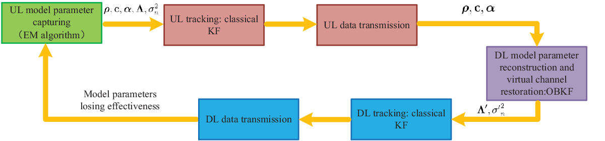
Refer to caption
Fig. 4: The algorithm block diagram of the proposed scheme.
Algorithm 2 UL Learning Aided DL Reconstruction and Restoration
1:  input: 𝐲,p⁡(θ),𝐲~′​(m)\mathbf{y},p(\theta),\tilde{\mathbf{y}}^{\prime}(m).
2:  initialize: 𝜶^(0),𝚲^(0),𝐜^(0),𝝆^(0),σn2^(0),θ(0)∼π⁡(θ)\boldsymbol{\hat{\alpha}}^{(0)},\mathbf{\hat{\Lambda}}^{(0)},\mathbf{\hat{c}}^{(0)},\boldsymbol{\hat{\rho}}^{(0)},{\hat{\sigma_{n}^{2}}}^{(0)},\quad\theta^{(0)}\sim\pi(\theta).
3:  for l=0,1,…,ll=0,1,\ldots,l do
4:   𝐜^(l)←\mathbf{\hat{c}}^{(l)}\leftarrow Algorithm 1, [ρ^k(l)]j←(37)[\hat{\boldsymbol{\rho}}_{k}^{(l)}]_{j}\leftarrow\eqref{update_rho} and the constraint [ρk]j∈[−12,12][{\boldsymbol{\rho}}_{k}]_{j}\in[-\frac{1}{2},\frac{1}{2}].
5:   𝜶^(l)←(38),[𝚲^k]j,j(l)←(39),σn2^(l)←(40)\boldsymbol{\hat{\alpha}}^{(l)}\leftarrow\eqref{update_alpha},\quad[\hat{\boldsymbol{\Lambda}}_{k}]_{j,j}^{(l)}\leftarrow\eqref{update_Lambda},\quad{\hat{\sigma_{n}^{2}}}^{(l)}\leftarrow\eqref{update_sigma}.
6:  end for
7:  αk′←(48)\alpha_{k}^{\prime}\leftarrow\eqref{DL_alpha}, 𝒬k′,𝝆k′←(50),(51)\mathcal{Q}_{k}^{\prime},\boldsymbol{\rho}_{k}^{\prime}\leftarrow\eqref{angle reciprocity},\eqref{p' and rho}.
8:  [𝐠~^0]𝒬′ϑ←𝔼⁡{[𝐠~m]𝒬′ϑ},𝔼ϑ​[𝐏0ϑ|𝐲~′​(0)]←cov⁡[[𝐠~m]𝒬′ϑ][\widehat{\tilde{\mathbf{g}}}_{0}]_{\mathcal{Q}^{\prime}}^{\boldsymbol{\vartheta}}\leftarrow\mathbb{E}\left\{[{\tilde{\mathbf{g}}}_{m}]_{\mathcal{Q}^{\prime}}^{\boldsymbol{\vartheta}}\right\},\quad\mathbb{E}_{\boldsymbol{\vartheta}}[\mathbf{P}_{0}^{\boldsymbol{\vartheta}}|\tilde{\mathbf{y}}^{\prime}(0)]\leftarrow\mathrm{cov}\left[[{\tilde{\mathbf{g}}}_{m}]_{\mathcal{Q}^{\prime}}^{\boldsymbol{\vartheta}}\right].
9:  𝔼ϑ​{[𝚲′]𝒬′|𝐲~′​(0)}←𝔼ϑ​{[𝚲′]𝒬′},𝔼ϑ​{σn2′σp2​𝐈|𝒬′||𝐲~′​(0)}←𝔼ϑ​{σn2′σp2​𝐈|𝒬′|}\mathbb{E}_{\boldsymbol{\vartheta}}\left\{[\mathbf{\Lambda}^{\prime}]_{\mathcal{Q}^{\prime}}|\tilde{\mathbf{y}}^{\prime}(0)\right\}\leftarrow\mathbb{E}_{\boldsymbol{\vartheta}}\left\{[\mathbf{\Lambda}^{\prime}]_{\mathcal{Q}^{\prime}}\right\},\quad\mathbb{E}_{\boldsymbol{\vartheta}}\left\{\frac{\sigma_{n}^{2\prime}}{\sigma_{p}^{2}}\mathbf{I}_{|\mathcal{Q}^{\prime}|}|\tilde{\mathbf{y}}^{\prime}(0)\right\}\leftarrow\mathbb{E}_{\boldsymbol{\vartheta}}\left\{\frac{\sigma_{n}^{2\prime}}{\sigma_{p}^{2}}\mathbf{I}_{|\mathcal{Q}^{\prime}|}\right\}.
10:  for m=1,2,…m=1,2,\ldots do
11:   𝐳~mϑ←𝐲~m′ϑ−[𝐠~^m]𝒬′ϑ\tilde{\mathbf{z}}_{m}^{\boldsymbol{\vartheta}}\leftarrow\tilde{\mathbf{y}}_{m}^{\prime{\boldsymbol{\vartheta}}}-[\widehat{\tilde{\mathbf{g}}}_{m}]_{\mathcal{Q}^{\prime}}^{\boldsymbol{\vartheta}}.
12:   𝐊mΘ←𝔼ϑ​{𝐏mϑ|𝐲~′​(m−1)}​𝔼ϑ−1​{𝐏mϑ+σn2′σp2​𝐈|𝒬′||𝐲~′​(m−1)}\mathbf{K}_{m}^{\Theta}\leftarrow\mathbb{E}_{\boldsymbol{\vartheta}}\left\{\mathbf{P}_{m}^{\boldsymbol{\vartheta}}|\tilde{\mathbf{y}}^{\prime}(m-1)\right\}\mathbb{E}_{\boldsymbol{\vartheta}}^{-1}\left\{\mathbf{P}_{m}^{\boldsymbol{\vartheta}}+\frac{\sigma_{n}^{2\prime}}{\sigma_{p}^{2}}\mathbf{I}_{|\mathcal{Q}^{\prime}|}|\tilde{\mathbf{y}}^{\prime}(m-1)\right\}.
13:   for i=1,2,…,num_iterationsi=1,2,\ldots,\text{num\_iterations} do
14:    ϑ~∼p⁡(ϑ|ϑ(i−1))\tilde{\boldsymbol{\vartheta}}\sim p({\boldsymbol{\vartheta}}|{\boldsymbol{\vartheta}}^{(i-1)}).
15:    for j=2,3,…,m−1j=2,3,\ldots,m-1 do
16:     𝝂j←(σn2′σp2​𝐈|𝒬′|)−1​𝐲~j′+𝚺j−1​𝝁j,𝚪j←(α′2​[𝚲′]𝒬′−1+(σn2′σp2​𝐈|𝒬′|)−1+𝚺j−1)−1\bm{\nu}_{j}\leftarrow\left(\frac{\sigma_{n}^{2\prime}}{\sigma_{p}^{2}}\mathbf{I}_{|\mathcal{Q}^{\prime}|}\right)^{-1}\tilde{\mathbf{y}}_{j}^{\prime}+\mathbf{\Sigma}_{j}^{-1}\boldsymbol{\mu}_{j},\kern 10.0pt\mathbf{\Gamma}_{j}\leftarrow\left(\alpha^{\prime 2}[\mathbf{\Lambda}^{\prime}]_{\mathcal{Q}^{\prime}}^{-1}+(\frac{\sigma_{n}^{2\prime}}{\sigma_{p}^{2}}\mathbf{I}_{|\mathcal{Q}^{\prime}|})^{-1}+\mathbf{\Sigma}_{j}^{-1}\right)^{-1}.
17:     𝚺j+1←([𝚲′]𝒬′−1−α′2​[𝚲′]𝒬′−1​𝚪j​[𝚲′]𝒬′−1)−1\boldsymbol{\Sigma}_{j+1}\leftarrow\left([\bm{\Lambda}^{\prime}]_{\mathcal{Q}^{\prime}}^{-1}-\alpha^{\prime 2}[\bm{\Lambda}^{\prime}]_{\mathcal{Q}^{\prime}}^{-1}\bm{\Gamma}_{j}[\bm{\Lambda}^{\prime}]_{\mathcal{Q}^{\prime}}^{-1}\right)^{-1}.
18:     𝝁j+1←α′​𝚺j+1​[𝚲′]𝒬′−1​𝚪j​((σn2′σp2​𝐈|𝒬′|)−1​𝐲~j′+𝚺j−1​𝝁j)\bm{\mu}_{j+1}\leftarrow\alpha^{\prime}\bm{\Sigma}_{j+1}[\bm{\Lambda}^{\prime}]_{\mathcal{Q}^{\prime}}^{-1}\bm{\Gamma}_{j}\left(\left(\frac{\sigma_{n}^{2\prime}}{\sigma_{p}^{2}}\mathbf{I}_{|\mathcal{Q}^{\prime}|}\right)^{-1}\tilde{\mathbf{y}}_{j}^{\prime}+\mathbf{\Sigma}_{j}^{-1}\boldsymbol{\mu}_{j}\right).
19:     ωj+1←using(70)\omega_{j+1}\leftarrow\text{using}\eqref{omega_i+1}.
20:    end for
21:    𝚫m−1←(σn2′σp2​𝐈|𝒬′|)−1+𝚺m−1,𝐆m←𝚫m​((σn2′σp2​𝐈|𝒬′|)−1​𝐲~m′+𝚺m−1​𝝁m)\mathbf{\Delta}_{m}^{-1}\leftarrow\left(\frac{\sigma_{n}^{2\prime}}{\sigma_{p}^{2}}\mathbf{I}_{|\mathcal{Q}^{\prime}|}\right)^{-1}+\mathbf{\Sigma}_{m}^{-1},\quad\mathbf{G}_{m}\leftarrow\mathbf{\Delta}_{m}\left((\frac{\sigma_{n}^{2\prime}}{\sigma_{p}^{2}}\mathbf{I}_{|\mathcal{Q}^{\prime}|})^{-1}\tilde{\mathbf{y}}_{m}^{\prime}+\mathbf{\Sigma}_{m}^{-1}\boldsymbol{\mu}_{m}\right).
22:    p⁡(𝐲~′​(m)|ϑ)←using(IV-B2),p⁡(ϑ~|𝐲~′​(m))←p⁡(𝐲~′​(m)|ϑ)p(\tilde{\mathbf{y}}^{\prime}(m)|{\boldsymbol{\vartheta}})\leftarrow\text{using}\eqref{y|theta},\quad p(\tilde{\boldsymbol{\vartheta}}|\tilde{\mathbf{y}}^{\prime}(m))\leftarrow p(\tilde{\mathbf{y}}^{\prime}(m)|{\boldsymbol{\vartheta}}).
23:    r←min​{1,p⁡(𝐲~′​(m)|ϑ~)​p​(ϑ~)p⁡(𝐲~′​(m)|ϑ(i−1))​p​(ϑ(i−1))},ζ∼unif​(0,1)r\leftarrow\text{min}\{1,\frac{p(\tilde{\mathbf{y}}^{\prime}(m)|\tilde{\boldsymbol{\vartheta}})p(\tilde{\boldsymbol{\vartheta}})}{p(\tilde{\mathbf{y}}^{\prime}(m)|{\boldsymbol{\vartheta}}^{(i-1)})p({\boldsymbol{\vartheta}}^{(i-1)})}\},\quad\zeta\sim\text{unif}(0,1).
24:    if ζ<r\zeta<r then
25:     ϑ(i)←ϑ~{\boldsymbol{\vartheta}}^{(i)}\leftarrow{\tilde{\boldsymbol{\vartheta}}}.
26:    else
27:     ϑ(i)←ϑ(i−1){\boldsymbol{\vartheta}}^{(i)}\leftarrow{\boldsymbol{\vartheta}}^{(i-1)}.
28:    end if
29:   end for
30:   𝔼ϑ​{σn2′σp2​𝐈|𝒬′||𝐲~′​(m)},𝔼ϑ​{[𝚲′]𝒬′|𝐲~′​(m)}←{ϑ(1),ϑ(2),…​ϑ(m)}\mathbb{E}_{\boldsymbol{\vartheta}}\left\{\frac{\sigma_{n}^{2\prime}}{\sigma_{p}^{2}}\mathbf{I}_{|\mathcal{Q}^{\prime}|}|\tilde{\mathbf{y}}^{\prime}(m)\right\},\mathbb{E}_{\boldsymbol{\vartheta}}\left\{[\mathbf{\Lambda}^{\prime}]_{\mathcal{Q}^{\prime}}|\tilde{\mathbf{y}}^{\prime}(m)\right\}\leftarrow\{{\boldsymbol{\vartheta}}^{(1)},{\boldsymbol{\vartheta}}^{(2)},\ldots{\boldsymbol{\vartheta}}^{(m)}\}.
31:   𝔼ϑ{𝐏m+1ϑ|𝐲~′(m)}←α′2(𝐈−𝐊mΘ∗)𝔼ϑ{𝐏mϑ|𝐲~′(m)}+𝔼ϑ{[𝚲′]𝒬′|𝐲~′(m)}\mathbb{E}_{\boldsymbol{\vartheta}}\left\{\mathbf{P}_{m+1}^{\boldsymbol{\vartheta}}|\tilde{\mathbf{y}}^{\prime}(m)\right\}\leftarrow\alpha^{\prime 2}(\mathbf{I}-\mathbf{K}_{m}^{\Theta*}\mathbf{)}\mathbb{E}_{\boldsymbol{\vartheta}}\left\{\mathbf{P}_{m}^{\boldsymbol{\vartheta}}|\tilde{\mathbf{y}}^{\prime}(m)\right\}+\mathbb{E}_{\boldsymbol{\vartheta}}\Big\{[\mathbf{\Lambda}^{\prime}]_{\mathcal{Q}^{\prime}}|\tilde{\mathbf{y}}^{\prime}(m)\Big\}.
32:   [𝐠~^m+1]𝒬′ϑ←α′​[𝐠~^m]𝒬′ϑ+α′​𝐊mΘ​𝐳~mϑ[\widehat{\tilde{\mathbf{g}}}_{{m+1}}]_{\mathcal{Q}^{\prime}}^{\boldsymbol{\vartheta}}\leftarrow\alpha^{\prime}[\widehat{\tilde{\mathbf{g}}}_{m}]_{\mathcal{Q}^{\prime}}^{\boldsymbol{\vartheta}}+\alpha^{\prime}\mathbf{K}_{m}^{\Theta}\tilde{\mathbf{z}}_{m}^{\boldsymbol{\vartheta}}.
33:   return [𝐠~^m+1]𝒬′ϑ[\widehat{\tilde{\mathbf{g}}}_{{m+1}}]_{\mathcal{Q}^{\prime}}^{\boldsymbol{\vartheta}}.
34:  end for

V Simulations Results

In this section, we will evaluate the performance of our proposed tracking scheme through numerical simulation. We consider a massive MIMO network where the BS is equipped with Nt=128N_{t}=128 antennas. K=32K=32 is the number of users, while they are divided into 88 groups. We take the first group as an example to show the perfect performance. The simulation parameters are summarized in TABLE 1.

TABLE I: Simulation Parameters
Number of BS antennas NtN_{t} 128
Number of users per group τ\tau 4
angle spread range [−49∘−43∘],[−26∘−20∘],[-49^{\circ}-43^{\circ}],[-26^{\circ}-20^{\circ}],
[20∘​26∘],[43∘​49∘][20^{\circ}26^{\circ}],[43^{\circ}49^{\circ}]
Length of training sequences LtL_{t} 4
Channel coherence interval LcL_{c} 160
Symbol period 1 us
Carrier frequency 2 GHz
BS antenna space λ/2\lambda/2

Correspondingly, the preamble is also divided into 88 segments. Only 44 users in the same group are active tt each segment, so there is no inter-group interference. As a result, the training of length 4 is sufficient. During the virtual channel tracking stage, the KK users are regrouped such that the spatial signatures of the users in the same group do not overlap. The signal-to-noise ratio (SNR) is defined as SNR=σp2/σn2=\sigma_{p}^{2}/\sigma_{n}^{2}. The performance metrics are taken as the average MSEs of the model parameters α\alpha, 𝐜\mathbf{c} and 𝚲\mathbf{\Lambda} and that of the virtual channel 𝐠~\tilde{\mathbf{g}} and 𝐡~\tilde{\mathbf{h}} i.e.,

MSE𝐱=\displaystyle\text{MSE}_{\mathbf{x}}= 1τ​∑i=1τ‖𝐱^i−𝐱i‖2‖𝐱i‖2,𝐱=α,𝐜,𝚲,𝝆,σn2,𝐡~,𝐠~.\displaystyle\frac{1}{\tau}\sum_{i=1}^{\tau}\frac{\|\hat{\mathbf{x}}_{i}-\mathbf{x}_{i}\|^{2}}{\|\mathbf{x}_{i}\|^{2}},{\mathbf{x}}=\alpha,\mathbf{c},\mathbf{\Lambda},\boldsymbol{\rho},\sigma_{n}^{2},\tilde{\mathbf{h}},\tilde{\mathbf{g}}. (85)
Refer to caption
Fig. 5: The convergence of the EM based UL model parameter learning algorithm with SNR = 30dB.

We first investigate the convergence of the UL EM process. Fig. 5 shows the MSEs curves versus the number of iteration. Mu=15M_{u}=15 channel blocks are used to learn model parameters. We can see from Fig. 5 that after 5 iterations, all the parameters have arrived at their steady states, which shows that the algorithm has a fast convergence speed.

Refer to caption
Refer to caption
Fig. 6: (a) The MSE performance of the UL model parameters learning versus SNR. (b) The off-grid bias and spatial signature performance with SNR = 20dB.

Fig. 6 presents the MSE performance of the model parameters learning as a function of SNR, with EM algorithm running 5 iterations for each SNR case. With the increase of the SNR, we can see that the MSE curves of all parameters decrease almost linearly. Moreover, we show the performance of the estimation for the off-grid bias and spatial signature performance in Fig. 6, with SNR = 20dB. They are also estimated very accurately.

After UL learning of all parameters and DL reconstruction of partial parameters, the next step is to track the DL channel by adopt OBKF, with the known parameters, meanwhile restore the unreconstructed parameters for later tracking. To decrease the computation complexity, we will adopt OBKF for a limited number of time-blocks, and then use classical KF to continue tracking the channel.

Refer to caption
Fig. 7: The MSE of the DL channel model parameters versus OBKF blocks MdM_{d}.
Refer to caption
Fig. 8: The MSE of the DL virtual channel model parameters versus SNR.

First, we studies the MSE of the two unknown DL channel model parameters at the last OBKF time-block versus the number of time-block using OBKF, with different SNR, and the MSE versus SNR with different number of OBKF time-block. In Fig. 7, we can see that the MSE of the two unknown DL channel model parameters decreases in each SNR case, and almost arrive at their convergence point when OBKF time-block Md=15M_{d}=15. As SNR goes higher, the convergence point can be arrived when OBKF time-block Md=10M_{d}=10. We can also see that the curves linearly decrease with the increase of the SNR, in Fig. 8.

We can find that the performance are better when SNR is higher. we can explain the above phenomenon that OBKF is not only restoring the virtual channel, but also restoring the unknown parameters. And after a scale of restoring time, the parameters will be very closed to the true one, so the estimated virtual channel will have a good performance.

Refer to caption
Fig. 9: The MSE of the DL virtual channel for each tracking blocks mdm_{d}.

Then we studied the MSE of virtual channel for each time-block, including both the OBKF time-blocks and the later classical KF time-blocks, with different SNR, as shown in Fig. 9. The figure also shows the performance of classical KF with perfect parameters as well as classical KF with weak parameters. We set the number of OBKF time-block Md=10M_{d}=10, with which we can obtain almost the best performance. From Fig. 9 we can obtain that the MSE of tracked virtual channel decreases when OBKF runs. We can see that the performance to be steady and is very close to the performance of classical KF with perfect parameters at md=6m_{d}=6, which shows the accuracy of our method.

Refer to caption
Fig. 10: The MSE of the DL virtual channel versus SNR.

To further illustrate the performance of the method, Fig. 10 shows the relationship between MSE of virtual channel and SNR, together with classical KF of the above two situations. from Fig. 10 we can see that the performance of KF with weak parameters is far away from the precisely one, while our OBKF method has a wonderful performance. Moreover, with the SNR increasing, the gap between our method and perfect KF decreases very fast. At SNR = 30, for example, the two performance is very nearly equal. Notice that the gap between our method and weak KF is also decreasing. This can be explained as follows. At low SNR, our method obtains a huge gain by utilizing the correlation of time-varying channel. But with SNR increasing, the performance is mostly decided on SNR, meanwhile the effect of correlation is diminishing.

Refer to caption
Fig. 11: The MSE of the DL virtual channel model parameters for different velocity.

Furthermore, we show the MSE performance of the two unknown DL channel model parameters versus SNR for different velocity at the last OBKF time-block, while Md=15M_{d}=15. In Fig. 11, we can find that the performance is better at slower velocity, while at higher velocity the performance is only a little worse and is acceptable.

VI Conclusion

In this paper, we proposed a skillful scheme for the DL channel tracking. First, with the help of VCR, a dynamic uplink (UL) massive MIMO channel model was built with the consideration of off-grid refinement. Then, a coordinate-wise maximization based expectation maximization (EM) algorithm was adopted in the model parameters learning period. Thanks to the angle reciprocity, with the knowledge of UL channel model parameters, we recovered some of the parameters of DL channel model. After that, as there remains some parameters which could not be perfectly inferred from the UL ones, we resorted to OBKF method to accurately track the DL channel. During the method, factor-graph and Metropolis Hastings MCMC were applied to track the expectation of posterior statistics. Numerical results showed that our proposed scheme has not only a strong convergence, but also a very low estimation MSE.

VII Appendix
The product of the NN-dimensional complex Gaussian PDF

For the NN-dimensional complex Gaussian distribution p⁡(𝐱)=𝒞​𝒩​(𝒙,𝝁,𝚺)p(\mathbf{x})=\mathcal{CN}\left({\boldsymbol{x};\boldsymbol{\mu},\boldsymbol{\Sigma}}\right), we can obtain its canonical notation as

p⁡(𝐱)=\displaystyle p(\mathbf{x})= 1πN​|𝚺|​exp⁡(−(𝐱−𝝁)H​𝚺−1​(𝐱−𝝁))\displaystyle\frac{1}{\pi^{N}|\boldsymbol{\Sigma}|}\exp(-(\mathbf{x}-\boldsymbol{\mu})^{H}\boldsymbol{\Sigma}^{-1}(\mathbf{x}-\boldsymbol{\mu}))
=\displaystyle= exp⁡(−ln⁡πN−ln⁡|𝚺|)​exp​{−𝐱H​𝚺−1​𝐱−𝝁H​𝚺−1​𝝁+2​ℜ​{𝐱H​𝚺−1​𝝁}}\displaystyle\exp(-\ln\pi^{N}-\ln|\boldsymbol{\Sigma}|)\exp\left\{-\mathbf{x}^{H}\boldsymbol{\Sigma}^{-1}\mathbf{x}-\boldsymbol{\mu}^{H}\boldsymbol{\Sigma}^{-1}\boldsymbol{\mu}+2\Re\{\mathbf{x}^{H}\boldsymbol{\Sigma}^{-1}\boldsymbol{\mu}\}\right\}
=\displaystyle= exp⁡(−N​ln⁡π−ln⁡|𝚺|−𝝁H​𝚺−1​𝝁−𝐱H​𝚺−1​𝐱+2​ℜ⁡{𝐱H​𝚺−1​𝝁}).\displaystyle\exp({-N\ln\pi-\ln|\boldsymbol{\Sigma}|-\boldsymbol{\mu}^{H}\boldsymbol{\Sigma}^{-1}\boldsymbol{\mu}}-\mathbf{x}^{H}\boldsymbol{\Sigma}^{-1}\mathbf{x}+2\Re\{\mathbf{x}^{H}\boldsymbol{\Sigma}^{-1}\boldsymbol{\mu}\}). (86)

Then, for the PDFs pi​(𝐱)=𝒞​𝒩​(𝒙,𝝁i,𝚺i)p_{i}(\mathbf{x})=\mathcal{CN}\left({\boldsymbol{x};\boldsymbol{\mu}_{i},\boldsymbol{\Sigma}_{i}}\right), i=1,2,…,Li=1,2,\ldots,L, we can derive

∏i=1Lpi​(𝐱)=\displaystyle\prod_{i=1}^{L}p_{i}(\mathbf{x})= ∏i=1L𝒞​𝒩​(𝒙,𝝁i,𝚺i)\displaystyle\prod_{i=1}^{L}\mathcal{CN}\left({\boldsymbol{x};\boldsymbol{\mu}_{i},\boldsymbol{\Sigma}_{i}}\right)
=\displaystyle= exp⁡(∑i=1Lζi−𝐱H​(∑i=1L𝚺i−1)​𝐱+2​ℜ⁡{𝐱H​(∑i=1L𝚺i−1​𝝁i)}),\displaystyle\exp\left(\sum_{i=1}^{L}\zeta_{i}-\mathbf{x}^{H}\left(\sum_{i=1}^{L}\boldsymbol{\Sigma}_{i}^{-1}\right)\mathbf{x}+2\Re\left\{\mathbf{x}^{H}\left(\sum_{i=1}^{L}\boldsymbol{\Sigma}^{-1}_{i}\boldsymbol{\mu}_{i}\right)\right\}\right), (87)

where the term ζi=−N​ln⁡π−ln⁡|𝚺i|−𝝁iH​𝚺i−1​𝝁i\zeta_{i}=-N\ln\pi-\ln|\boldsymbol{\Sigma}_{i}|-\boldsymbol{\mu}_{i}^{H}\boldsymbol{\Sigma}^{-1}_{i}\boldsymbol{\mu}_{i} is defined in the above equation. Before proceeding, let us define 𝚺¯L=(∑i=1L𝚺i−1)−1\boldsymbol{\bar{\Sigma}}_{L}=\left(\sum_{i=1}^{L}\boldsymbol{\Sigma}_{i}^{-1}\right)^{-1}, and 𝝁¯L=𝚺¯L​(∑i=1L𝚺i−1​𝝁i)\boldsymbol{\bar{\mu}}_{L}=\boldsymbol{\bar{\Sigma}}_{L}\left(\sum\limits_{i=1}^{L}\boldsymbol{\Sigma}^{-1}_{i}\boldsymbol{\mu}_{i}\right). Hence, the above equation can be reexpressed as

∏i=1Lpi​(𝐱)=\displaystyle\prod_{i=1}^{L}p_{i}(\mathbf{x})= exp⁡(∑i=1Lζi−𝐱H​𝚺¯L−1​𝐱+2​ℜ⁡{𝐱H​𝚺¯L−1​𝝁¯L})\displaystyle\exp\left(\sum_{i=1}^{L}\zeta_{i}-\mathbf{x}^{H}\boldsymbol{\bar{\Sigma}}_{L}^{-1}\mathbf{x}+2\Re\left\{\mathbf{x}^{H}\boldsymbol{\bar{\Sigma}}_{L}^{-1}\boldsymbol{\bar{\mu}}_{L}\right\}\right)
=\displaystyle= exp⁡(∑i=1Lζi−ζ¯L+ζ¯L−𝐱H​𝚺¯L−1​𝐱+2​ℜ⁡{𝐱H​𝚺¯L−1​𝝁¯L})\displaystyle\exp\left(\sum_{i=1}^{L}\zeta_{i}-\bar{\zeta}_{L}+\bar{\zeta}_{L}-\mathbf{x}^{H}\boldsymbol{\bar{\Sigma}}_{L}^{-1}\mathbf{x}+2\Re\left\{\mathbf{x}^{H}\boldsymbol{\bar{\Sigma}}_{L}^{-1}\boldsymbol{\bar{\mu}}_{L}\right\}\right)
=\displaystyle= exp⁡(∑i=1Lζi−ζ¯L)​𝒞​𝒩​(𝐱,𝝁¯L,𝚺¯L),\displaystyle\exp\left(\sum_{i=1}^{L}\zeta_{i}-\bar{\zeta}_{L}\right)\mathcal{CN}\left(\mathbf{x};\boldsymbol{\bar{\mu}}_{L},\boldsymbol{\bar{\Sigma}}_{L}\right), (88)

where ζ¯L=−N​ln⁡π−ln⁡|𝚺¯L|−𝝁¯LH​𝚺¯L−1​𝝁¯L\bar{\zeta}_{L}=-N\ln\pi-\ln|\boldsymbol{\bar{\Sigma}}_{L}|-\boldsymbol{\bar{\mu}}_{L}^{H}\boldsymbol{\bar{\Sigma}}_{L}^{-1}\boldsymbol{\bar{\mu}}_{L}.

Specially, for L=2L=2, it can be obtained that

exp⁡(∑i=12ζi−ζ¯2)=𝒞​𝒩​(𝟎,𝝁1,𝚺1)​𝒞​𝒩​(𝟎,𝝁2,𝚺2)𝒞​𝒩​(𝟎,(𝚺1−1+𝚺2−1)−1​(𝚺1−1​𝝁1+𝚺2−1​𝝁2),(𝚺1−1+𝚺2−1)−1).\displaystyle\exp\left(\sum_{i=1}^{2}\zeta_{i}-\bar{\zeta}_{2}\right)=\frac{\mathcal{CN}(\mathbf{0};\boldsymbol{\mu}_{1},\boldsymbol{\Sigma}_{1})\mathcal{CN}(\mathbf{0};\boldsymbol{\mu}_{2},\boldsymbol{\Sigma}_{2})}{\mathcal{CN}\left(\mathbf{0};(\boldsymbol{\Sigma}_{1}^{-1}+\boldsymbol{\Sigma}_{2}^{-1})^{-1}\left(\boldsymbol{\Sigma}_{1}^{-1}\boldsymbol{\mu}_{1}+\boldsymbol{\Sigma}_{2}^{-1}\boldsymbol{\mu}_{2}\right),(\boldsymbol{\Sigma}_{1}^{-1}+\boldsymbol{\Sigma}_{2}^{-1})^{-1}\right)}. (89)

Moreover, if the terms 𝝁1\bm{\mu}_{1}, 𝚺1\bm{\Sigma}_{1}, 𝝁¯2\bm{\bar{\mu}}_{2}, and 𝚺¯2\bm{\bar{\Sigma}}_{2} are given, we can derive the quotient of two N-dimensional complex Gaussian PDF

𝒞​𝒩​(𝐱,𝝁¯2,𝚺¯2)𝒞​𝒩​(𝐱,𝝁1,𝚺1)=𝒞​𝒩​(𝐱,(𝚺¯2−1−𝚺1−1)−1​(𝚺¯2−1​𝝁¯2−𝚺1−1​𝝁1),(𝚺¯2−1−𝚺1−1)−1)\displaystyle\frac{\mathcal{CN}(\mathbf{x};\bm{\bar{\mu}}_{2},\bm{\bar{\Sigma}}_{2})}{\mathcal{CN}(\mathbf{x};\bm{\mu}_{1},\bm{\Sigma}_{1})}=\mathcal{CN}\left(\mathbf{x};\left(\bm{\bar{\Sigma}}_{2}^{-1}-\bm{\Sigma}_{1}^{-1}\right)^{-1}\left(\bm{\bar{\Sigma}}_{2}^{-1}\bm{\bar{\mu}}_{2}-\bm{\Sigma}_{1}^{-1}\bm{\mu}_{1}\right),\left(\bm{\bar{\Sigma}}_{2}^{-1}-\bm{\Sigma}_{1}^{-1}\right)^{-1}\right)
×𝒞​𝒩​(𝟎,𝝁¯2,𝚺¯2)𝒞​𝒩​(𝟎,𝝁1,𝚺1)​𝒞​𝒩​(𝟎,(𝚺¯2−1−𝚺1−1)−1​(𝚺¯2−1​𝝁¯2−𝚺1−1​𝝁1),(𝚺¯2−1−𝚺1−1)−1).\displaystyle\kern 10.0pt\times\frac{\mathcal{CN}(\mathbf{0};\bm{\bar{\mu}}_{2},\bm{\bar{\Sigma}}_{2})}{\mathcal{CN}(\mathbf{0};\bm{\mu}_{1},\bm{\Sigma}_{1})\mathcal{CN}\left(\mathbf{0};\left(\bm{\bar{\Sigma}}_{2}^{-1}-\bm{\Sigma}_{1}^{-1}\right)^{-1}\left(\bm{\bar{\Sigma}}_{2}^{-1}\bm{\bar{\mu}}_{2}-\bm{\Sigma}_{1}^{-1}\bm{\mu}_{1}\right),\left(\bm{\bar{\Sigma}}_{2}^{-1}-\bm{\Sigma}_{1}^{-1}\right)^{-1}\right)}. (90)

References

  • [1] T. L. Marzetta, “Noncooperative Cellular Wireless with Unlimited Numbers of Base Station Antennas,” IEEE Trans. Wireless Commun., vol. 9, no. 11, pp. 3590–3600, Nov. 2010.
  • [2] F. Rusek, D. Persson, B. K. Lau, E. G. Larsson, T. L. Marzetta, O. Edfors, and F. Tufvesson, “Scaling up MIMO: Opportunities and challenges with very large arrays,” IEEE Signal Process. Mag., vol. 30, no. 1, pp. 40–60, Jan. 2013.
  • [3] V. Jungnickel, K. Manolakis, W. Zirwas, B. Panzner, V. Braun, M. Lossow, M. Sternad, R. Apelfrojd, and T. Svensson, “The role of small cells, coordinated multipoint, and massive MIMO in 5G,” IEEE Commun. Mag., vol. 52, no. 5, pp. 44–51, May 2014.
  • [4] X. Liu and Y. Liu and X. Wang and H. Lin, “Highly Efficient 3-D Resource Allocation Techniques in 5G for NOMA-Enabled Massive MIMO and Relaying Systems,” IEEE Journal on Selected Areas in Commun., vol. 35, no. 12, pp. 2785–2797, Dec. 2017.
  • [5] W. Tan, M. Matthaiou, S. Jin, and X. Li, “Spectral efficiency of DFT-based processing hybrid architectures in massive MIMO” IEEE Wireless Commun. Letters, vol. 6, no. 5, pp. 586-589 Oct. 2017.
  • [6] N. Jindal, “MIMO broadcast channels with finite-rate feedback,” IEEE Trans. Inf. Theory, vol. 52, no. 11, pp. 5045–5060, Nov. 2006.
  • [7] X. Yang, W.-J. Lu, N. Wang, K. Nieman, S. Jin, H. Zhu, X. Mu, I. Wong, Y. Huang, and X. You, “Design and implementation of a TDD-based 128-antenna massive MIMO prototyping system,” arXiv preprint arXiv:1608.07362, 2016.
  • [8] S. Noh, M. D. Zoltowski, and D. J. Love, “Training sequence design for feedback assisted hybrid beamforming in massive MIMO systems,” IEEE Trans. Commun., vol. 64, no. 1, pp. 187–200, Jan. 2016.
  • [9] L. Fan, S. Jin, CK. Wen, H. Zhang, “Uplink achievable rate for massive MIMO systems with low-resolution ADC,” IEEE Communications Letters., vol. 19, no. 12, pp. 2186-2189, 2015.
  • [10] H. Xie, F. Gao, and S. Jin, “An overview of low-rank channel estimation for massive mimo systems,” IEEE Access, vol. 4, pp. 7313–7321, Nov. 2016.
  • [11] S. Jin, X. Wang, Z. Li, KK. Wong, Y. Huang, X. Tang, “On massive MIMO zero-forcing transceiver using time-shifted pilots,” IEEE Transactions on Vehicular Technology., vol. 65, no. 1, pp. 59-74, 2016.
  • [12] A. Adhikary, J. Nam, J.-Y. Ahn, and G. Caire, “Joint spatial division and multiplexing the large-scale array regime,” IEEE Trans. Inf. Theory, vol. 59, no. 10, pp. 6441–6463, Oct. 2013.
  • [13] J. Nam, A. Adhikary, J. Y. Ahn, and G. Caire, “Joint spatial division and multiplexing: Opportunistic beamforming, user grouping and simplified downlink scheduling,” IEEE J. Sel. Topics Signal Process., vol. 8, no. 5, pp. 876–890, Oct. 2014.
  • [14] A. Adhikary, E. A. Safadi, M. K. Samimi, R. Wang, G. Caire, T. S. Rappaport, and A. F. Molisch, “Joint spatial division and multiplexing for mm-Wave channels,” IEEE J. Sel. Areas Commun., vol. 32, no. 6, pp. 1239–1255, Jun. 2014.
  • [15] C. Sun, X. Gao, S. Jin, M. Matthaiou, Z. Ding, and C. Xiao, “Beam division multiple access transmission for massive MIMO communications,” IEEE Trans. Commun., vol. 63, no. 6, pp. 2170–2184, Jun. 2015.
  • [16] H. Xie, F. Gao, S. Jin, J. Fang and Y. Liang, “Channel Estimation for TDD/FDD Massive MIMO Systems With Channel Covariance Computing,” IEEE Trans. Wireless Commun., vol. 17, no. 6, pp. 4206–4218, June. 2018.
  • [17] A. Decurninge, M. Guillaud and D. T. M. Slock, “Channel Covariance Estimation in Massive MIMO Frequency Division Duplex Systems,” 2015 IEEE Globecom Workshops (GC Wkshps), pp. 1–6, Dec. 2015.
  • [18] J. Ma, S. Zhang, H, Li, N. Zhao and V. C. M. Leung, “Interference-Alignment and Soft-Space-Reuse Based Cooperative Transmission for Multi-cell Massive MIMO Networks,” IEEE Trans. Wireless Commun., vol. 17, no. 3, pp. 1907-1922, Mar. 2018.
  • [19] H. Xie, F. Gao, S. Zhang, and S. Jin, “A Unified Transmission Strategy for TDD/FDD Massive MIMO Systems With Spatial Basis Expansion Model,” IEEE Trans. Veh. Technol., vol. 66, no. 4, pp. 3170–3184, Apr. 2017.
  • [20] H. Tang, J. Wang and L. He, “Off-Grid Sparse Bayesian Learning Based Channel Estimation for MmWave Massive MIMO Uplink,” IEEE Wireless Commun. Letters, pp. 1-1, June, 2018
  • [21] J. Zhao, F. Gao, W. Jia, J. Zhao, and W. Zhang, “Channel tracking for massive MIMO systems with spatial-temporal basis expansion model,” in Proc. 2017 IEEE International Conference on Communications (ICC), May 2017, pp. 1–5.
  • [22] J. Ma, S. Zhang, H. Li, F. Gao, and S. Jin, “Sparse Bayesian Learning for the Time-varying Massive MIMO Channels: Acquisition and Tracking,” IEEE Trans. on. Commun., pp. 1-1, 2018.
  • [23] A. M. Sayeed, “Deconstructing multiantenna fading channels,” IEEE Trans. Signal Process., vol. 50, no. 10, pp. 2563–2579, Oct. 2002.
  • [24] R. Dehghannasiri M. S. Esfahani and E. R. Dougherty, “Intrinsically Bayesian Robust Kalman Filter: An Innovation Process Approach,” IEEE Trans. Signal Process., vol. 65, no. 10, pp. 2531–2546, May. 2017.
  • [25] R. Dehghannasiri M. S. Esfahani X. Qian and E. R. Dougherty, “Optimal Bayesian Kalman Filtering With Prior Update,” IEEE Trans. Signal Process., vol. 66, no. 8, pp. 1982–1996, Apr. 201.
  • [26] L. You, X. Gao, A. L. Swindlehurst, and W. Zhong, “Channel acquisition for massive MIMO-OFDM with adjustable phase shift pilots.” IEEE Trans. Signal Process., vol. 64, no. 6, pp. 1461–1476, Mar. 2016.
  • [27] B. H. Fleury, “First- and second-order characterization of direction dispersion and space selectivity in the radio channel,” IEEE Trans. Inf. Theory, vol. 46, no. 6, pp. 2027–2044, Sept. 2000.
  • [28] K. Liu, V. Raghavan, and A. M. Sayeed, “Capacity scaling and spectral efficiency in wide-band correlated MIMO channels,” IEEE Trans. Inf. Theory, vol. 49, no. 10, pp. 2504–2526, Oct. 2003.
  • [29] J. Zhao, F. Gao, W. Jia, S. Zhang, S. Jin, and H. Lin, “Angle domain hybrid precoding and channel tracking for millimeter wave massive MIMO systems,” IEEE Trans. Wireless Commun., vol. 16, no. 10, pp. 6868–6880, Oct. 2017.
  • [30] Z. Gao, L. Dai, Z. Wang, and S. Chen, “Spatially common sparsity based adaptive channel estimation and feedback for FDD massive MIMO,” IEEE Trans. Signal Process., vol. 63, no. 23, pp. 6169–6183, Dec. 2015.
  • [31] Q. Zhang and S. A. Kassam, “Finite-state markov model for rayleigh fading channels,” IEEE Trans. Commun., vol. 47, no. 11, pp. 1688–1692, Nov. 1999.
  • [32] P. Parvazi and A. B. Gershman, “Direction-of-arrival and spatial signature estimation in antenna arrays with pairwise sensor calibration,” 2010 IEEE International Conference on Acoustics, Speech and Signal Processing, pp. 2618–2621, Mar. 2010.
  • [33] R. Prasad and C. R. Murthy, “Bayesian learning for joint sparse OFDM channel estimation and data detection,” in Proc. 2010 IEEE Global Telecommunications Conference, GLOBECOM 2010, Dec. 2010, pp. 1–6.
  • [34] D. P. Wipf and B. D. Rao, “Sparse bayesian learning for basis selection,” IEEE Trans. Signal Process., vol. 52, no. 8, pp. 2153–2164, 2004.
  • [35] T. Kailath, A. H. Sayed, and B. Hassibi, Linear estimation. Prentice Hall Upper Saddle River, NJ, USA, 2000.
  • [36] P. Data, “Prediction methods for the planning of indoor radiocommunication systems and radio local area networks in the frequency range 900 mhz to 100 ghz,” ITU-R Std, 2001.
  • [37] M. METIS, “wireless communications enablers for the twentytwenty information society, eu 7th framework programme project,” ICT-317669-METIS, Tech. Rep.
  • [38] F. R. Kschischang and B. J. Frey and H. Loeliger, “Factor graphs and the sum-product algorithm,” IEEE Trans. on Information Theory, vol. 47, no. 2, pp. 498–519, Feb. 2001.
  • [39] Christopher M. Bishop, Pattern Recognition and Machine Learning (Information Science and Statistics), Springer, 2016.