Improving and Understanding
Variational Continual Learning

Siddharth Swaroop Affiliation: University of Cambridge, UK, {ss2163,vcn22,ret26}@cam.ac.uk Cuong V. Nguyen Affiliation: University of Cambridge, UK, {ss2163,vcn22,ret26}@cam.ac.uk Thang D. Bui Affiliation: University of Sydney, Australia, thang.buivn@gmail.com Richard E. Turner Affiliation: University of Cambridge, UK, {ss2163,vcn22,ret26}@cam.ac.uk

Abstract

In the continual learning setting, tasks are encountered sequentially. The goal is to learn whilst i) avoiding catastrophic forgetting, ii) efficiently using model capacity, and iii) employing forward and backward transfer learning. In this paper, we explore how the Variational Continual Learning (VCL) framework achieves these desiderata on two benchmarks in continual learning: split MNIST and permuted MNIST. We first report significantly improved results on what was already a competitive approach. The improvements are achieved by establishing a new best practice approach to mean-field variational Bayesian neural networks. We then look at the solutions in detail. This allows us to obtain an understanding of why VCL performs as it does, and we compare the solution to what an ‘ideal’ continual learning solution might be.¹¹ 1 Code is available at https://github.com/nvcuong/variational-continual-learning/tree/master/improved_ddm

1 Introduction

In the real world, inputs can change over time, suffering from covariate and dataset shift, and often the size of datasets or privacy constraints make revisiting old data computationally prohibitive. Continual learning, where we receive data in an online fashion, allowing tasks to change and be added over time, focusses on these types of problems. An ideal continual learning solution (model and inference scheme) would, when it first sees data, efficiently use the model’s capacity to solve the task, without any forgetting of contributions from old data. Once the model has reached capacity, continual learning would adjust parameters such that the ‘least important’ information from old tasks is forgotten, and that backward and forward transfer learning is achieved: new data can be useful for increasing performance on old tasks (backward transfer), and information from old tasks can be used to perform better on new tasks (forward transfer).

We shall specifically focus on the continual image classification setting, a standard continual learning problem tackled in research. For the rest of this paper we will consider data arriving in batches as ‘tasks’, as opposed to data arriving in a fully online or sequential manner, which is the most general form of continual learning (even though our method can be applied in this fully online setting too). Due to their success on full-batch image classification, neural networks are often employed. However, naive techniques such as vanilla neural networks suffer from catastrophic forgetting [7, 13]. There have been many continual learning methods introduced to combat forgetting, and we consider them to be broadly split into three groups: methods that change the model architecture, methods which use rehearsal or past data, and methods which focus on the inference scheme (see section 2).

In this paper, we consider the Variational Continual Learning (VCL) framework [14], a method which focusses on the inference scheme, but which can also be combined with a rehearsal based method by incorporating coresets. Previous inference based approaches often do not maintain accurate parameter uncertainty estimates after training on each task. Uncertainty is extremely useful in deciding the important information from previous tasks, allowing for less important information to be forgotten. A Bayesian approach to learning parameters should automatically keep uncertainty estimates, and so should perform well in the continual learning setting. We therefore consider learning a Bayesian neural network, where we set the posterior from the previous task as the prior for a new task. Exact Bayesian inference is not tractable, and so we approximate the posterior after every task. Although some of the previous inference based approaches are closely related to approximate inference in a Bayesian neural network, we optimise the variational objective function. Variational Inference (VI) is known to provide better uncertainty estimates that other approaches in this setting [2].

We first summarise related work in Section 2. We introduce the VCL algorithm in Section 3, and report improved results on multi-head split MNIST and permuted MNIST (both with and without coresets). In Section 4, we look in detail at the solutions we obtained. This leads to some valuable insights on the behaviour we might expect from a ‘good’ continual learning model, both in terms of model capacity usage and forward/backward transfer, while also shedding some light on properties of mean-field variational Bayesian neural networks. Finally, we provide conclusions in Section 5.

2 Related work

Here we characterise the fast-growing universe of continual learning methods in terms of three orthogonal approaches: methods that change the model architecture, methods which use rehearsal or past data, and methods which focus on the inference scheme. These approaches are complementary and so they are often combined.

Model based approaches to continual learning. A conceptually simple method that changes model architecture is Progressive Neural Networks [17], which trains a new model (neural network) for each new task, using connections between old tasks’ models and newer tasks’ models to incorporate forward transfer [17]. However, the overall model grows linearly in size with task, and is therefore not efficient in terms of model capacity. It also does not have potential for backward transfer. It does, however, provide extremely good results on many benchmarks. A method similar in flavour is Continual Learning via Network Pruning [6], where they now regularise during training to automatically prune out a large part of the network after every task. This method therefore handles the model capacity problem much more elegantly, but still suffers when model capacity is reached, and does not have potential for backward transfer. We shall discuss pruning more in Section 4.

Rehearsal and memory based approaches to continual learning. Rehearsal of past data can be used to combat catastrophic forgetting. For example, Deep Generative Replay [19], inspired by the human brain, trains a generative model on each task’s data, and uses it to generate pseudo-data that is used in training in future tasks. More recently, this idea has been made more efficient by integrating the generative model into the training procedure [21]. Other examples of rehearsal based methods assume that a coreset of past data can be stored and used in the future [14, 15]. Note that storing any past data is a relaxation of the strictest continual learning problem (and may not be possible when, for example, strict privacy laws apply to past data).

Inference based approaches to continual learning. The third set of approaches regularise parameter updates by penalising against changes in ‘important’ parameters for previous tasks. For example, Elastic Weight Consolidation (EWC) [10, 16] regularises using Fisher information matrices from previous tasks. Synaptic Intelligence (SI) [22] compares the (rate of change of) the objective’s gradient and the parameters to decide each parameter’s importance to previous tasks, and EWC and SI can be combined [3]. Variational continual learning without coresets is also a pure inference based approach to continual learning.

Mixed approaches. It seems likely that using some combination of the three approaches to continual learning will provide the best methods. Indeed, VCL with coresets is such a mixed approach. Similarly, Progress & Compress [18] use concepts from Progressive Neural Networks [17] and EWC [10]. They train an active column on each new task (with some layerwise connections to the ‘knowledge base’), which is then distilled into a knowledge base, using a modified version of EWC to prevent catastrophic forgetting.

3 Improvements to Variational Continual Learning

VCL adopts a Bayesian approach to learning parameters of a model, using the previous task’s posterior as the new task’s prior when we see new data. VCL approximates each task’s posterior by a variational distribution, $q_{t}(\mathbf{\theta})\approx p_{t}(\mathbf{\theta|\mathcal{D}_{1:t}})$ , obtained by using Monte Carlo variational inference [1], maximising the objective (for every task $t$ )

\mathcal{L}_{t}(q_{t}(\mathbf{\theta}))=\sum_{n=1}^{N_{t}}\mathbb{E}_{\mathbf{\theta}\sim q_{t}(\mathbf{\theta})}\left[\log{p(y_{t}^{(n)}|\mathbf{\theta},\mathbf{x}_{t}^{(n)}})\right]-\mathcal{K}\mathcal{L}\left(q_{t}(\mathbf{\theta})||q_{t-1}(\mathbf{\theta})\right).

(1)

There are two terms in Equation 1, which we shall refer to as the likelihood term (the left hand term with Monte Carlo estimates), and the $\mathcal{K}\mathcal{L}$ term. For further details on the optimisation process, please see the original VCL paper [14]. We consider fully-connected multi-layer perceptrons in this paper, with ReLU activation functions, and use a Gaussian mean-field approximation over each of the weights, as in the original paper. We place a standard normal Gaussian over each parameter as the initial prior ( $p_{0}(\mathbf{\theta})$ ), and can calculate the $\mathcal{K}\mathcal{L}$ term in Equation 1 analytically. We use ADAM [8] to optimise for the means and variances of each parameter. For tests with episodic memory enhancement (coresets), we treat coresets the same way as in Nguyen et al. 2018, and randomly choose the examples in the coreset (the ‘random coreset’ method). We remove the (randomly selected) coreset images while training on the rest of the data, and train on only the coreset images just before test-time.

3.1 Improved results

We established a simple scheme for substantially improving results over Nguyen et al. 2018. Crucially, we optimise for a much longer time. Although progress can sometimes appear to stall during optimisation, in reality progress is just extremely slow. We also firstly introduce the local reparameterisation trick during the Monte Carlo sampling of the network [9], and secondly initialise all weights with small, random means (of the order $10^{-1}$ ) and small variances (of the order $10^{-3}$ ) before every task. Without these additional two tricks, we would have to wait for much longer in order to reach convergence. Although these improvements may seem technically trivial, we find that they are practically very important, greatly impacting results.

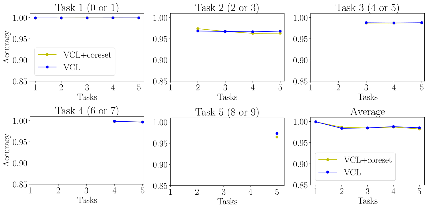
In the multi-head split MNIST task, we have to sequentially solve five binary classification tasks from the MNIST dataset: {0v1}, {2v3}, {4v5}, {6v7}, {8v9}. The challenge in split MNIST is to obtain good performance on new tasks while retaining performance on old ones. We ran a one hidden layer model with 200 units for 600 epochs (with 256 batch size), sharing the lower level weights between tasks, and report the mean and standard deviation over 10 runs. See Table 1 for results. Without coresets, we achieve a final test accuracy of 98.5 $\pm$ 0.4%, an increase from 97.0% reported earlier [14]. With coresets, we achieve 98.2 $\pm$ 0.4%, similar to the 98.4% reported earlier.

We also consider permuted MNIST. In permuted MNIST, we receive tasks sequentially, where each task is the standard (10-way) MNIST classification task, with the pixels having undergone a fixed random permutation, different for each task. Ideally, a network with two or more hidden layers would use lower layer(s) to ‘de-permute’ the images, and higher layer(s) to solve MNIST, which is then constant between tasks. We ran a two hidden layer model with 100 units in each hidden layer for 800 epochs (with 1024 batch size), and report the mean and standard deviation over 5 runs. Without coresets, this achieves a final average test accuracy of 93 $\pm$ 1%, as compared to 90% reported earlier [14] (Table 2). With coresets, we achieve a final average test accuracy of 94.6 $\pm$ 0.3%, as compared to 93% reported earlier. For reference, training the same network but seeing all the data together (batch mode) has an accuracy of 97% (this is an upper bound on the performance possible with this model and inference scheme).

Table 1: Final average test accuracy on multi-head split MNIST. VCL: Variational Continual Learning, EWC: Elastic Weight Consolidation, SI: Synaptic Intelligence. Results for EWC and SI are taken from Nguyen et al. 2018.

Method	Split MNIST	Split MNIST + 40 random coreset
VCL (this paper)	98.5 $\pm$ 0.4%	98.2 $\pm$ 0.4%
Previous VCL [14]	97.0%	98.4%
EWC [10]	63.1%	-
SI [22]	98.9%	-

4 Discussion

We now look into how VCL continually learns tasks, exploring how it uses its model capacity, primarily by looking at the learnt weights in the network.

4.1 Split MNIST

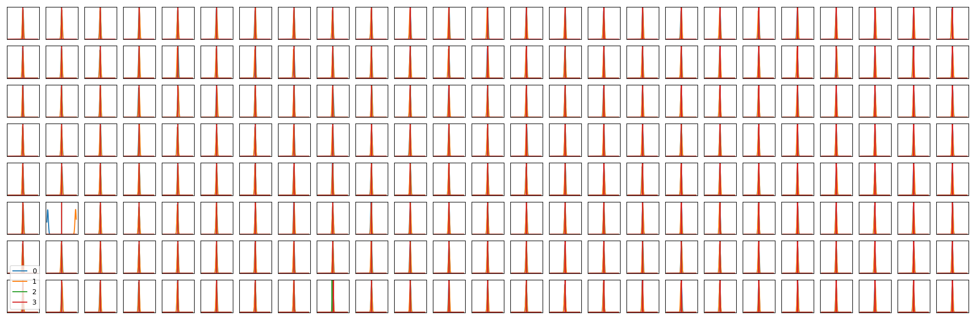
We first consider the model trained without coresets (although exactly the same effects happen with coresets). Appendix B shows plots of weights into and out of each unit after training on each task. Even though we have 200 units in the single hidden layer, it appears as if only one unit is being used per each of the five tasks; the remaining units are pruned out as part of the optimisation process. These active (un-pruned) units are plotted in Figure 1. This effect is similar to that observed in Trippe and Turner 2018, with entire units pruned out, as opposed to just individual weights. The pruned units appear to have input weights at or near the prior (standard normal Gaussian), with output weights near a delta function (zero mean, small variance), therefore minimising their effect on the output prediction. Removing all pruned units from the network does not change the network’s predictions (and therefore accuracy).

This pruning effect seems to be due to the choice of inference scheme. We leave a detailed review of the pruning process for future work, including characterising the mechanism and explaining it mathematically. Intuitively, the pruning effect can be explained by looking at the optimisation function (Equation 1). By reducing the effect of a unit on the output prediction (setting output weights to have zero mean and small variance), the input weights to the unit can be set to their prior. The increase in the $\mathcal{K}\mathcal{L}$ term due to the small variance of the output weights are offset by the reduction in the $\mathcal{K}\mathcal{L}$ term from the numerically more input weights. Provided the likelihood term does not change too much, a pruned solution is therefore more optimal. In this paper, we now focus on what our pruned solutions reveal about how our model approaches continual learning tasks, and debate whether the pruning effect is a feature or a bug for continual learning.

Refer to caption — Figure 1: The active units learnt during split MNIST, without coresets. Rows correspond to stages of continual learning. Left: means, Centre: variances, Right: output weights for each task’s two classes. Exactly the same effect is observed when incorporating coresets.

As the model only uses 1 hidden unit per task, it has learnt to use a fraction of its total capacity to successfully learn binary classifications in the split MNIST experiment. The high test accuracies indicate this is an efficient use of model capacity. Remaining, unused units can be used for other tasks that we may see in the future. This implies that pruning is a beneficial feature for continual learning, forcing the model to efficiently use its capacity.

Additionally, the pruning effect allows us to see some forward and backward transfer (see Figure 1), both important qualities in a good continual learning solution. Forward transfer is visible when previous tasks’ active units have non-zero weights for subsequent tasks. For example, unit 2, which was learnt after task 2 (classifying digits {2v3}), has non-zero output weights after task 4 (classifying {6v7}). The model therefore uses some information about the task {2v3} in solving the task {6v7}. Although less visible in the plots, there is also backward transfer in the same units: unit 2’s input weights change slightly after training on task 4 ({6v7}), potentially changing test accuracy on task 2. In this case however, any backward transfer does not result in different test accuracies; this could be because there is no potential for improvement given the high test accuracies involved.

The exact same effects are seen when we train the model with coresets: the same pruning effect appears (Figure 1 and the figures in Appendix B are similar when trained with coresets), and similar test accuracies are obtained (within one standard deviation). This shows that for a simple task such as multi-head split MNIST, there is no need for incorporating coresets.

This pruning effect is also similar to that considered in Golkar et al. 2019, where they prune out entire units. However, they have hyperparameters that control the degree of pruning (and corresponding accuracy loss). Previous work on Variational Inference for BNNs has found that VI methods can be used to prune large parts of the network [12], and we show here how this pruning is done over units as opposed to weights (see also Trippe and Turner 2018). In comparison to Golkar et al. 2019, our method automatically prunes out entire units, and is able to re-use the units for both forward and backward transfer.

4.2 Permuted MNIST

We now look into how the two hidden layer model approaches permuted MNIST (results in Table 2). We first consider the model trained without coresets. Appendix C shows figures of the weights, showing there is still pruning. The numbers of active (un-pruned) units after training on each task are summarised in Figure 2.

There are more active units in permuted MNIST than were in split MNIST, perhaps due to the more difficult nature of permuted MNIST (classifying between 10 digits, as opposed to between 2). However, only 11 units are used in the second hidden layer, with the remaining 89 units pruned out. Additionally, the output weights on these 11 units do not change between tasks (see Appendix C for weights for training without coresets; the figures with coresets look the same). This confirms that the hidden layers effectively de-permute the images, allowing the output weights to just classify between the 10 digits.

Beyond re-using the upper level weights, there is not much evidence of forward or backward transfer. We should expect this from permuted MNIST because the network trains on all MNIST digits on the first task itself, hence already learning the ‘best’ way to classify between MNIST digits. Any subsequent permuted images cannot improve this. Instead, the remaining focus of permuted MNIST seems to be on ensuring we use available model capacity as efficiently as possible. Increasing the model capacity improves results: training a network with 250 units in the lower hidden layer (instead of 100) improves final average test accuracy to 95.5% (10 tasks).

Incorporating coresets also improves results. However, the number of active units (plotted in Figures 2) and the weight plots (in Appendix C) look the same. Instead, training VCL with coresets (which can be viewed as changing the order in which the model trains on data, or, changing the schedule with which we visit training data) appears to reinforce previous tasks’ images: it lowers forgetting in the network.

Table 2: Final average test accuracy on permuted MNIST for various methods (results taken from respective papers). A hidden layer size of {

n_{1},n_{2}

} indicates two hidden layers, the lower hidden layer having

n_{1}

hidden units, the upper hidden layer having

n_{2}

(followed by a softmax over the 10 MNIST classes). Methods with an asterisk (*) use some sort of episodic memory. Results marked with a double asterisk (**) were read from a graph in the source paper.

Method/Paper	Hidden layer size	Number of tasks	Final average test accuracy
VCL (this paper)	{100, 100}	10	93 $\pm$ 1%
VCL + 200 random coreset (this paper)	{100, 100}	10	94.6 $\pm$ 0.3%
Previous VCL [14]	{100, 100}	10	90%
Previous VCL + 200 random coreset [14]	{100, 100}	10	93%
Kronecker-factored Laplace [16]	{100, 100}	50	90%
Kronecker-factored Laplace [16]	{100, 100}	10	96%**
EWC [10]	{2000, 2000}	10	97%
EWC [10] (result from [14])	{100, 100}	10	84%
SI [22]	{2000, 2000}	10	97%
SI [22] (result from [14])	{100, 100}	10	86%
Continual Learning via Neural Pruning [6]	{2000, 2000}	10	98.42 $\pm$ 0.04%
A-GEM [4]	{256, 256}	20	89.1 $\pm$ 0.14%
A-GEM [4]	{256, 256}	10	92.3%**
GEM [11]	{100, 100}	20	80%
BLLL-REG [5]	{100, 100}	10	92.2%
GEM [11] (result from [4])	{256, 256}	20	89.5 $\pm$ 0.48%
GEM [11] (result from [4])	{256, 256}	10	93.1%**
Riemannian Walk [3] (result from [4])	{256, 256}	20	85.7 $\pm$ 0.56%
Riemannian Walk [3] (result from [4])	{256, 256}	10	91.6%**
Progressive NNs [17] (result from [4])	{256, 256}	20	93.5 $\pm$ 0.07%
Progressive NNs [17] (result from [4])	{256, 256}	10	94.6%**

Table 2 summarises some recent works’ results on permuted MNIST. As can be seen, different papers use different numbers of hidden units in their hidden layers, and test over different numbers of tasks. However, as the findings in this paper indicate, permuted MNIST primarily tests for model capacity, highlighting how we cannot faithfully compare results when model capacity and number of tasks differ. We propose that when using permuted MNIST as a benchmark in continual learning, model capacity is kept fairly limited (for example, two hidden layers with either 100 or 256 hidden units each), and number of tasks is kept high (minimum 10, possibly more). Of all methods, Ritter et al. 2018 achieves significantly superior results, as they use a relatively small network and test over many tasks. Note that 2000 units in two hidden layers is an extremely large model for 10 tasks: as Golkar et al. 2019 note, they can achieve high (as good as single-task) performance having pruned out a large proportion of their network. With such a large model capacity, this benchmark no longer tests any desiderata in continual learning aside from avoiding catastrophic forgetting, which many other benchmarks can also do.

Many papers often use permuted MNIST to demonstrate how their method (and other baseline methods) exhibit some of continual learning’s desiderata. For example, they show some form of resistance to forgetting or efficient use of model capacity via metrics or plots. In this case, comparing the final average test accuracy is no longer so important, but we believe far better comparisons would be achieved if a more challenging hidden layer size and number of tasks was used.

5 Conclusions and future work

This paper has significantly improved the performance of Variational Continual Learning [14] on split MNIST and permuted MNIST. It has also shed light on the mechanism that VCL employs to counter catastrophic forgetting. Future work would involve applying VCL to other, harder benchmarks, where there is more potential for forward and backward transfer. It should also explore the observed pruning effect, a consequence of using mean-field variational Bayesian neural networks. Another avenue for future work would be to consider structured approximations to the distribution over parameters (we currently only consider the mean-field approximation), which can potentially improve results in continual learning [16].

References

Blundell et al. [2015] C. Blundell, J. Cornebise, K. Kavukcuoglu, and D. Wierstra. Weight uncertainty in neural network. In F. Bach and D. Blei, editors, Proceedings of the 32nd International Conference on Machine Learning, volume 37 of Proceedings of Machine Learning Research, pages 1613–1622, Lille, France, 07–09 Jul 2015. PMLR. URL http://proceedings.mlr.press/v37/blundell15.html.
Bui et al. [2016] T. Bui, D. Hernandez-Lobato, J. Hernandez-Lobato, Y. Li, and R. Turner. Deep gaussian processes for regression using approximate expectation propagation. In M. F. Balcan and K. Q. Weinberger, editors, Proceedings of The 33rd International Conference on Machine Learning, volume 48 of Proceedings of Machine Learning Research, pages 1472–1481, New York, New York, USA, 20–22 Jun 2016. PMLR. URL http://proceedings.mlr.press/v48/bui16.html.
Chaudhry et al. [2018] A. Chaudhry, P. K. Dokania, T. Ajanthan, and P. H. S. Torr. Riemannian walk for incremental learning: Understanding forgetting and intransigence. CoRR, abs/1801.10112, 2018. URL http://arxiv.org/abs/1801.10112.
Chaudhry et al. [2019] A. Chaudhry, M. Ranzato, M. Rohrbach, and M. Elhoseiny. Efficient lifelong learning with a-GEM. In International Conference on Learning Representations, 2019. URL https://openreview.net/forum?id=Hkf2_sC5FX.
Ebrahimi et al. [2019] S. Ebrahimi, M. Elhoseiny, T. Darrell, and M. Rohrbach. Uncertainty-guided lifelong learning in bayesian networks, 2019. URL https://openreview.net/forum?id=SJMBM2RqKQ.
Golkar et al. [2019] S. Golkar, M. Kagan, and K. Cho. Continual learning via neural pruning. CoRR, abs/1903.04476, 2019. URL http://arxiv.org/abs/1903.04476.
Goodfellow et al. [2014] I. J. Goodfellow, M. Mirza, D. Xiao, A. Courville, and Y. Bengio. An Empirical Investigation of Catastrophic Forgetting in Gradient-Based Neural Networks. In International Conference on Learning Representations, 2014. URL http://arxiv.org/abs/1312.6211.
Kingma and Ba [2014] D. P. Kingma and J. Ba. Adam: A method for stochastic optimization. CoRR, abs/1412.6980, 2014. URL http://arxiv.org/abs/1412.6980.
Kingma et al. [2015] D. P. Kingma, T. Salimans, and M. Welling. Variational Dropout and the Local Reparameterization Trick. In C. Cortes, N. D. Lawrence, D. D. Lee, M. Sugiyama, and R. Garnett, editors, Advances in Neural Information Processing Systems 28, pages 2575–2583. Curran Associates, Inc., 2015. URL http://papers.nips.cc/paper/5666-variational-dropout-and-the-local-reparameterization-trick.pdf.
Kirkpatrick et al. [2017] J. Kirkpatrick, R. Pascanu, N. Rabinowitz, J. Veness, G. Desjardins, A. A. Rusu, K. Milan, J. Quan, T. Ramalho, A. Grabska-Barwinska, D. Hassabis, C. Clopath, D. Kumaran, and R. Hadsell. Overcoming catastrophic forgetting in neural networks. Proceedings of the National Academy of Sciences, 2017, 2017. URL http://arxiv.org/abs/1612.00796. arXiv: 1612.00796.
Lopez-Paz and Ranzato [2017] D. Lopez-Paz and M. A. Ranzato. Gradient episodic memory for continual learning. In I. Guyon, U. V. Luxburg, S. Bengio, H. Wallach, R. Fergus, S. Vishwanathan, and R. Garnett, editors, Advances in Neural Information Processing Systems 30, pages 6467–6476. Curran Associates, Inc., 2017. URL http://papers.nips.cc/paper/7225-gradient-episodic-memory-for-continual-learning.pdf.
Louizos et al. [2017] C. Louizos, K. Ullrich, and M. Welling. Bayesian compression for deep learning. In I. Guyon, U. V. Luxburg, S. Bengio, H. Wallach, R. Fergus, S. Vishwanathan, and R. Garnett, editors, Advances in Neural Information Processing Systems 30, pages 3288–3298. Curran Associates, Inc., 2017. URL http://papers.nips.cc/paper/6921-bayesian-compression-for-deep-learning.pdf.
Mccloskey and Cohen [1989] M. Mccloskey and N. J. Cohen. Catastrophic interference in connectionist networks: The sequential learning problem. The Psychology of Learning and Motivation, 24:104–169, 1989.
Nguyen et al. [2018] C. V. Nguyen, Y. Li, T. D. Bui, and R. E. Turner. Variational continual learning. In International Conference on Learning Representations, 2018. URL https://openreview.net/forum?id=BkQqq0gRb.
Rebuffi et al. [2017] S. Rebuffi, A. Kolesnikov, G. Sperl, and C. H. Lampert. icarl: Incremental classifier and representation learning. In 2017 IEEE Conference on Computer Vision and Pattern Recognition, CVPR 2017, Honolulu, HI, USA, July 21-26, 2017, pages 5533–5542, 2017. doi: 10.1109/CVPR.2017.587. URL https://doi.org/10.1109/CVPR.2017.587.
Ritter et al. [2018] H. Ritter, A. Botev, and D. Barber. Online structured laplace approximations for overcoming catastrophic forgetting. In S. Bengio, H. Wallach, H. Larochelle, K. Grauman, N. Cesa-Bianchi, and R. Garnett, editors, Advances in Neural Information Processing Systems 31, pages 3738–3748. Curran Associates, Inc., 2018. URL http://papers.nips.cc/paper/7631-online-structured-laplace-approximations-for-overcoming-catastrophic-forgetting.pdf.
Rusu et al. [2016] A. A. Rusu, N. C. Rabinowitz, G. Desjardins, H. Soyer, J. Kirkpatrick, K. Kavukcuoglu, R. Pascanu, and R. Hadsell. Progressive neural networks. CoRR, abs/1606.04671, 2016. URL http://arxiv.org/abs/1606.04671.
Schwarz et al. [2018] J. Schwarz, J. Luketina, W. M. Czarnecki, A. Grabska-Barwinska, Y. W. Teh, R. Pascanu, and R. Hadsell. Progress & Compress: A scalable framework for continual learning. ICML 2018, May 2018. URL http://arxiv.org/abs/1805.06370. arXiv: 1805.06370.
Shin et al. [2017] H. Shin, J. K. Lee, J. Kim, and J. Kim. Continual learning with deep generative replay. In I. Guyon, U. V. Luxburg, S. Bengio, H. Wallach, R. Fergus, S. Vishwanathan, and R. Garnett, editors, Advances in Neural Information Processing Systems 30, pages 2990–2999. Curran Associates, Inc., 2017. URL http://papers.nips.cc/paper/6892-continual-learning-with-deep-generative-replay.pdf.
Trippe and Turner [2018] B. Trippe and R. Turner. Overpruning in Variational Bayesian Neural Networks. arXiv:1801.06230 [stat], Jan. 2018. URL http://arxiv.org/abs/1801.06230. arXiv: 1801.06230.
van der Ven and Tolias [2018] G. M. van der Ven and A. S. Tolias. Generative replay with feedback connections as a general strategy for continual learning. CoRR, abs/1809.10635, 2018. URL http://arxiv.org/abs/1809.10635.
Zenke et al. [2017] F. Zenke, B. Poole, and S. Ganguli. Continual learning through synaptic intelligence. In D. Precup and Y. W. Teh, editors, Proceedings of the 34th International Conference on Machine Learning, volume 70 of Proceedings of Machine Learning Research, pages 3987–3995, International Convention Centre, Sydney, Australia, 06–11 Aug 2017. PMLR. URL http://proceedings.mlr.press/v70/zenke17a.html.

Appendix A

This appendix has figures showing the test accuracy after training on split MNIST and permuted MNIST, both with and without coresets.

Appendix B

This appendix has figures showing the means and variances of weights after training without coresets on each of the five tasks in split MNIST (MLP with 1 hidden layers, 200 hidden units).

Appendix C

This appendix has figures showing the means and variances of weights after training without coresets on tasks 1, 5 and 10 on permuted MNIST (MLP with 2 hidden layers, 100 units in each layer, 10 tasks total).