Detecting Orbital Angular Momentum of Light in Satellite-to-Ground Quantum Communications

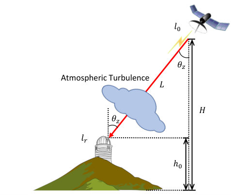
In this work, we consider the scenario of satellite-to-ground quantum communications which is illustrated in Fig. (1). Here we briefly introduce our system settings. A satellite (at an altitude of $H$ and a zenith angle of $\theta_{z}$) sends an OAM eigenstate with the original OAM quantum number $l_{0}$ to the ground station (whose altitude is $h_{0}$) through an atmospheric channel (with a channel distance of $L$). For a higher-dimensional quantum encoding, $l_{0}$ can be chosen from a Hilbert space, $\{-l_{\rm{max}},\ldots,+l_{\rm{max}}\}$, whose dimension is $(2l_{\rm{max}}+1)$. The ground station performs a quantum measurement on the received state and obtains a result $l_{r}$. Throughout this paper, we assume $\theta_{z}<45\degree$ as discussed in [35] in order to satisfy the condition that the atmospheric turbulence within the satellite-to-ground atmospheric channel is weak. We denote the aperture radius at the transmitter and the receiver as $r_{t}$ and $r_{a}$, respectively.

In cylindrical coordinates, the general form of an OAM eigenstate¹¹ 1 Note, in this work our OAM-beams are in fact classical solutions to Maxwell’s equations, and in this sense ‘classical’ states. Even though we will use some formalism from quantum mechanics in our calculations, none of the states we investigate will have negative Wigner functions (e.g. entangled states), and therefore are not formally ‘non-classical’ states. However, it can be shown that these solutions for OAM-beams map to single photons carrying $l\hbar$ of OAM and therefore form an eigenbasis for single-photon descriptions. is given by

$$\varphi_{p,l}(r,\theta,z)=R_{p,l}(r,z)\frac{\exp(il\theta)}{\sqrt{2\pi}},$$

(1)

where $r$ and $\theta$ are the radial and azimuthal coordinates, respectively, $z$ is the longitudinal coordinate, $l$ is the OAM quantum number, $p$ is the radial node number, and $R_{p,l}(r,z)$ is the radial profile. In general, OAM eigenstates with different $l$ values are mutually orthogonal. In this paper, we choose $R_{p,l}(r,z)$ to be Laguerre-Gauss functions, making OAM eigenstates correspond to the Laguerre-Gaussian ($LG$) mode set [13]. $R_{p,l}(r,z)$ can be expressed by

	$\displaystyle R_{p,l}(r,z)=$	$\displaystyle 2\sqrt{\frac{p!}{(p+|l|)!}}\frac{1}{w(z)}\left[\frac{r\sqrt{2}}{w(z)}\right]^{|l|}\exp\left[\frac{-r^{2}}{w^{2}(z)}\right]$		(2)
		$\displaystyle L_{p}^{|l|}\left(\frac{2r^{2}}{w^{2}(z)}\right)\exp\left[\frac{ikr^{2}z}{2\left(z^{2}+z_{R}^{2}\right)}\right]$
		$\displaystyle\exp\left[-i(2p+|l|+1)\tan^{-1}\left(\frac{z}{z_{R}}\right)\right],$

where $w(z)=w_{0}\sqrt{1+(z/z_{R})^{2}}$ with $w_{0}$ being the beam-waist radius, $z_{\mathrm{R}}=\pi w_{0}^{2}/\lambda$ is the Rayleigh range, $\lambda$ is the optical wavelength, $k=2\pi/\lambda$ is the optical wavenumber, and $L_{p}^{|l|}(x)$ is the generalized Laguerre polynomial [14]. In this work, we denote the $LG$ modes and their complex amplitudes as ${LG}_{pl}$, and we set $p=0$ for the transmitted OAM eigenstates, since OAM is only related to $l$.

In general, the power of an $LG_{0l}$ mode is distributed within an infinite transverse plane. However, in practice, we always have a finite aperture size at any transceiver. $LG_{0l}$ modes are single-ring annular modes whose maximum optical intensity is located at $r=\sqrt{|l|/2}w(z)$ [36], indicating an $l$-dependent beam size. In this work, we use a finite quantity, $r_{\textit{0l}}(z)$, within which most ($\sim 90\%$) of the optical power is distributed, to characterize the beam size of the $LG_{0l}$ mode. $r_{\textit{0l}}(z)$ is given by

$$r_{\textit{0l}}(z)=\sqrt{2}r_{\rm{rms}}^{\textit{{0l}}}(z),$$

(3)

where $r_{\rm{rms}}^{\textit{{0l}}}(z)$ is the rms beam radius, which can be evaluated by [37]

	$\displaystyle r_{\mathrm{rms}}^{\textit{{0l}}}(z)$	$\displaystyle=\sqrt{\int\!\!\!\!\int\!\varphi_{0,l}(r,\theta,z)\varphi_{0,l}^{*}(r,\theta,z)r\,\mathrm{d}r\mathrm{d}\theta}$		(4)
		$\displaystyle=\sqrt{\frac{|l|+1}{2}}w(z).$

In practice, the actual transmitter aperture radius $r_{t}$, and the actual receiver aperture radius $r_{a}$ should be set at least equal to $r_{0l}(0)$, and $r_{0l}(z)$, respectively.

In our system model, the transmitter aperture and the receiver aperture are situated at the points $z=0$ and $z=L$, respectively. The transmitted OAM eigenstate will be perturbed by the atmospheric turbulence while propagating. We denote the perturbed state at the ground station as $\Psi(r,\theta,z)$, which is generally a superposition of OAM eigenstates [25], thus is not orthogonal to any OAM eigenstate. Based on Born’s law, we express the conditional probability of obtaining a measurement $l_{r}$ as

$$P(l_{r}|\Psi)=\sum_{p}\left|a_{p,l_{r}}(z)\right|^{2}.$$

(5)

where $a_{p,l_{r}}(z)$ is the probability amplitude which is given by

$$a_{p,l_{r}}(z)=\left\langle\varphi_{p,l_{r}}|\Psi(r,\theta,z)\right\rangle.$$

(6)

The rotational field correlation (RFC) function of the received OAM-beam can be defined as [25]

$$C_{\Psi}(r,\theta,\theta^{\prime},z)=\left\langle\Psi^{*}(r,\theta^{\prime},z)\Psi(r,\theta,z)\right\rangle,$$

(7)

where $\theta$ and $\theta^{\prime}$ denote two arbitrary azimuthal coordinates at $r$ in the transverse plane, and $\langle...\rangle$ denotes an ensemble average. The unconditional probability of detecting $l_{r}$ can now be given by [25]

	$\displaystyle P(l_{r})=$	$\displaystyle\left\langle P(l_{r}|\Psi)\right\rangle$		(8)
	$\displaystyle=$	$\displaystyle\int\!\!\!\!\int\!\!\int\!C_{\Psi}(r,\theta,\theta^{\prime},z)rdr\frac{\exp\left[-il_{r}\left(\theta-\theta^{\prime}\right)\right]}{2\pi}d\theta^{\prime}d\theta.$

The probability $P(l_{0})$ gives the probability of correctly detecting $l_{0}$, and the probability $P(l_{r})$ gives the probability of detecting $l_{r}$ $(l_{r}\neq l_{0})$. In this work, when we refer to the ‘detection probability’, we will be referring to the value $P(l_{0})$. When we refer to the ‘crosstalk’ between OAM eigenstates, we shall be referring to the value $P(l_{r})$.

The effect of atmospheric turbulence on an optical beam manifests itself in both the beam’s intensity profile and the beam’s phase profile. The strength of the refractive index fluctuations within a satellite-based atmospheric channel can be characterized by the structure parameter $C_{n}^{2}(h)$. $C_{n}^{2}(h)$ can be described by the widely used Hufnagel-Valley (HV) model [38]

	$\displaystyle C_{n}^{2}(h)$	$\displaystyle=0.00594(v_{\rm{rms}}/27)^{2}\left(h\times 10^{-5}\right)^{10}\exp{(-h/1000)}$		(9)
		$\displaystyle+2.7\times 10^{-16}\exp{(-h/1500)}+A\exp{(-h/100)},$

where $h$ denotes the altitude, $v_{\rm{rms}}$ is the rms wind speed in m/s, and $A=C^{2}_{n}(0)$. In this work, we consider the Kolmogorov model [39] for the atmospheric turbulence.

The atmospheric turbulence leads to three effects on the intensity profile, namely beam wandering, beam broadening, and elliptical-shape beam deformation (as illustrated in Fig. (2)). These three effects were well described in [34] where good agreements were found with the experimental results in [40, 41, 42]. The three effects mentioned above are characterized by five random parameters, $\{r_{0},\phi_{0},W_{1},W_{2},\phi\}$. The parameters $\{r_{0},\phi_{0}\}$ characterize the centroid wandering of the beam, and $\{W_{1},W_{2},\phi\}$ characterize the elliptical-shape deformation and the broadening of the beam (see Fig. (2)). The distributions of these five parameters have been well established for non-OAM-beams using the Gaussian approximation under the assumption that the atmospheric turbulence is isotropic [34]. Specifically, $\phi$ is uniformly distributed over $[0,\pi/2)$, and is independent of the other parameters. The wandering beam-centroid position (in Cartesian coordinates), $x_{0}=r_{0}\cos{\phi_{0}}$ and $y_{0}=r_{0}\sin{\phi_{0}}$, can be considered as independent zero-mean Gaussian variables. Finally, $W_{1}$ and $W_{2}$ follow a multi-variable log-normal distribution. Denoting $\Theta_{1}=\ln{\frac{W_{1}^{2}}{w_{0}^{2}}}$, and $\Theta_{2}=\ln{\frac{W_{2}^{2}}{w_{0}^{2}}}$, $\{x_{0},y_{0},\Theta_{1},\Theta_{2}\}$ follow a joint Gaussian distribution with mean values of

$$\begin{gathered}\left\langle x_{0}\right\rangle=\left\langle y_{0}\right\rangle=0,\\ \left\langle\Theta_{1}\right\rangle=\left\langle\Theta_{2}\right\rangle=\ln\left[\frac{\left(1+2.96\sigma_{I}^{2}\Omega^{5/6}\right)^{2}}{\Omega^{2}\sqrt{\left(1+2.96\sigma_{I}^{2}\Omega^{5/6}\right)^{2}+1.2\sigma_{I}^{2}\Omega^{5/6}}}\right],\end{gathered}$$

(10)

and a covariance matrix of

$$\mathcal{M}=\left[\begin{array}[]{cccc}{\left\langle x_{0}^{2}\right\rangle}&{0}&{0}&{0}\\ {0}&{\left\langle y_{0}^{2}\right\rangle}&{0}&{0}\\ {0}&{0}&{\left\langle\Theta_{1}^{2}\right\rangle}&{\left\langle\Theta_{1}\Theta_{2}\right\rangle}\\ {0}&{0}&{\left\langle\Theta_{1}\Theta_{2}\right\rangle}&{\left\langle\Theta_{2}^{2}\right\rangle}\end{array}\right].$$

(11)

The elements in Eq. (10) and Eq. (11) are given by

	$\displaystyle\left\langle x_{0}^{2}\right\rangle=\left\langle y_{0}^{2}\right\rangle$	$\displaystyle=0.33w_{0}^{2}\sigma_{I}^{2}\Omega^{-7/6},$		(12)
	$\displaystyle\left\langle\Theta_{1}^{2}\right\rangle=\left\langle\Theta_{2}^{2}\right\rangle$	$\displaystyle=\ln\left[1+\frac{1.2\sigma_{I}^{2}\Omega^{5/6}}{\left(1+2.96\sigma_{I}^{2}\Omega^{5/6}\right)^{2}}\right],$
	$\displaystyle\left\langle\Theta_{1}\Theta_{2}\right\rangle$	$\displaystyle=\ln\left[1-\frac{0.8\sigma_{I}^{2}\Omega^{5/6}}{\left(1+2.96\sigma_{I}^{2}\Omega^{5/6}\right)^{2}}\right],$

where $\Omega={kw_{0}^{2}}/{2L}$ with $L$ being the propagation distance, and $\sigma_{I}^{2}$ is the scintillation index. For satellite-to-ground (downlink) channels, $\sigma_{I}^{2}$ can be calculated by [35]

$$\sigma_{I}^{2}=\exp\left[\frac{0.49\sigma_{R}^{2}}{\left(1+1.11\sigma_{R}^{12/5}\right)^{7/6}}+\frac{0.51\sigma_{R}^{2}}{\left(1+0.69\sigma_{R}^{12/5}\right)^{5/6}}\right]-1,$$

(13)

with $\sigma_{R}^{2}$ being the Rytov variance,

$$\sigma_{R}^{2}=2.25k^{7/6}\sec^{11/6}(\theta_{z})\int_{h_{0}}^{H}C_{n}^{2}(h)\left(h-h_{0}\right)^{5/6}dh.$$

(14)

A before-and-after comparison of the atmospheric turbulence effect on the intensity profile of the $LG_{04}$ mode is shown in Fig. (3) for illustration. Note that for the $LG_{0l}$ mode, $W_{1}$ and $W_{2}$ need to be scaled by a factor of $\sqrt{|l|+1}$ to faithfully characterize the beam divergence.

The atmospheric turbulence effect on the phase profile can be modeled as a single random phase screen $\alpha(r,\theta)$ in the receiver aperture plane [25]. The phase screen $\alpha(r,\theta)$ manifests itself as a phase perturbation term of $\exp{[i\alpha(r,\theta)]}$ in the complex amplitude of the modified beam. The function $\alpha(r,\theta)$ can be statistically characterized by its phase structure function

$$\mathcal{D}_{\alpha}(r,\theta,r^{\prime},\theta^{\prime})=\left\langle|\alpha(r,\theta)-\alpha(r^{\prime},\theta^{\prime})|^{2}\right\rangle,$$

(15)

where $(r,\theta)$ and $(r^{\prime},\theta^{\prime})$ denote two points in the aperture plane. $\mathcal{D}_{\alpha}(r,\theta,r^{\prime},\theta^{\prime})$ can be expressed in a simplified form of

$$\mathcal{D}_{\alpha}(r,\theta,r^{\prime},\theta^{\prime})=D_{\alpha}(|\Delta r|)=6.88\left(\frac{|\Delta r|}{r_{F}}\right)^{5/3},$$

(16)

where $\Delta r$ is the separation distance between $(r,\theta)$ and $(r^{\prime},\theta^{\prime})$, and $r_{F}$ is the well-known Fried parameter [43] that characterizes the phase coherence of the turbulent atmosphere. This parameter is given by [44]

$$r_{F}=\left[0.423k^{2}\sec\theta_{z}\int_{h_{0}}^{H}C_{n}^{2}(h)dh\right]^{-3/5},$$

(17)

for satellite-to-ground channels.

Considering the atmospheric turbulence effect introduced in Section III-A, we now express $\Psi(r,\theta,z)$ as

$$\Psi(r,\theta,z)=H(r)\Psi_{D}(r,\theta,z)\exp[i\alpha(r,\theta)].$$

(18)

In the above equation, $H(r)$ is the symmetrical circular aperture function which is given by

$$H(r)=\left\{\begin{array}[]{l}{1,\ \ \ r\leq r_{a}}\\ {0,\ \ \ r>r_{a}}\end{array},\right.$$

(19)

and $\Psi_{D}(r,\theta,z)$ is given by

$$\Psi_{D}(r,\theta,z)=\frac{\varphi_{0,l_{0}}(r_{i},\theta_{i},z)}{\sqrt{|\mathbf{S}|}},$$

(20)

where

$$\begin{gathered}\begin{aligned} r_{i}=&\sqrt{(x_{i})^{2}+(y_{i})^{2}},\\ \theta_{i}=&\atantwo(y_{i},x_{i}).\end{aligned}\end{gathered}$$

(21)

The parameters in Eq. (20) and Eq. (21) are given by

$$\left[\begin{array}[]{l}{x_{i}}\\ {y_{i}}\end{array}\right]=S^{-1}\left[\begin{array}[]{l}{x_{t}}\\ {y_{t}}\end{array}\right],$$

(22)

	$\displaystyle x_{t}$	$\displaystyle=r\cos\theta-r_{0}\cos\phi_{0},$		(23)
	$\displaystyle y_{t}$	$\displaystyle=r\sin\theta-r_{0}\sin\phi_{0},$

where $\mathbf{S}$ is a matrix that characterizes the beam shape, and it is given by

$$\mathbf{S}=\frac{1}{r_{0l_{0}}(z)}\left[\begin{matrix}{W_{1}\cos\phi}&{-W_{2}\sin\phi}\\ {W_{1}\sin\phi}&{\ \ W_{2}\cos\phi}\end{matrix}\right].$$

(24)

After expressing $\Psi(r,\theta,z)$ as Eq. (18), we are now in a position to evaluate $P(l_{0})$ and $P(l_{r})$. First, we substitute Eq. (18) into Eq. (7), and rewrite the RFC function as

	$\displaystyle C_{\Psi}(r,\theta,\theta^{\prime},z)$	$\displaystyle=\left\langle\Psi_{D}^{*}(r,\theta^{\prime},z)\Psi_{D}(r,\theta,z)\right\rangle$		(25)
		$\displaystyle\times C_{\alpha}(r,\theta,\theta^{\prime})\times H^{2}(r),$

where $C_{\alpha}(r,\theta,\theta^{\prime})$ is given by

$$C_{\alpha}(r,\theta,\theta^{\prime})=\langle\exp\{i[\alpha(r,\theta)-\alpha(r,\theta^{\prime})]\}\rangle.$$

(26)

Assuming the refractive index fluctuations to be a Gaussian random process so that $\langle\exp(ix)\rangle=\exp\left(-\frac{1}{2}\left\langle|x|^{2}\right\rangle\right)$ is true [25], we can express $C_{\alpha}(r,\theta,\theta^{\prime})$ as

	$\displaystyle C_{\alpha}(r,\theta,\theta^{\prime})=$	$\displaystyle\exp\!\left[-\frac{1}{2}D_{\alpha}\left(\left|2r\sin\left(\frac{\theta-\theta^{\prime}}{2}\right)\right|\right)\right]$		(27)
	$\displaystyle=$	$\displaystyle\exp\!\left[-6.88\!\times\!2^{2/3}\!\left(\!\frac{r}{r_{F}}\!\right)^{5/3}\!\left|\sin\left(\frac{\theta-\theta^{\prime}}{2}\right)\!\right|^{5/3}\right]\!\!.$

Substituting Eqs. (19), (20), (27) into Eq. (25), and then substituting Eq. (25) into Eq. (8), we can evaluate $P(l_{0})$ and $P(l_{r})$.

In this work, we carry out Monte Carlo simulations to evaluate $P(l_{0})$ and $P(l_{r})$. First, we generate a large number of realizations of the atmospheric turbulence by randomly generating their characterizing parameters $\{r_{0},\phi_{0},W_{1},W_{2},\phi\}$ following the distributions discussed in Section III-A. Then, for each realization we numerically evaluate $\Psi_{D}(r,\theta,z)$ and $C_{\alpha}(r,\theta,\theta^{\prime})$ to give $C_{\Psi}(r,\theta,\theta^{\prime},z)$. Note that while evaluating $C_{\alpha}(r,\theta,\theta^{\prime})$, $r_{F}$ is fixed, since $r_{F}$ is not dependent on specific realizations of the atmospheric turbulence (see Eq. (17)). Afterwards, realizations of $C_{\Psi}(r,\theta,\theta^{\prime},z)$ are used to obtain realizations of $P(l_{0})$ and $P(l_{r})$. At last, all realizations of $P(l_{0})$ and $P(l_{r})$ are averaged to give their final values.

In our simulation, we generate 2000 independent realizations of the atmospheric turbulence, and then evaluate the corresponding OAM detection performances. The final result of $P(l_{0})$ and $P(l_{r})$ is acquired by averaging over all the realizations.

For the system settings, we consider a vertical satellite-to-ground channel (i.e. $\theta_{z}=0$), and thus we have $H=h_{0}+L$. We restrict our study to the Low Earth Orbit (LEO) setting, and set the maximum satellite altitude to $H_{\rm{max}}=500\rm{km}$. We consider three cases of $h_{0}=0\rm{m}$, $h_{0}=1000\rm{m}$, and $h_{0}=3000\rm{m}$, giving maximum channel distances of $L_{\rm{max}}=500\rm{km}$, $L_{\rm{max}}=499\rm{km}$, and $L_{\rm{max}}=497\rm{km}$, respectively. For the atmospheric channel parameters, we set $C_{n}^{2}(0)=9.6\times 10^{-14}\mathrm{m}^{-2/3}$, and $v_{\rm{rms}}=6\rm{m/s}$. These atmospheric channel parameters accord with a realistic setting which was adopted in [45] to study satellite-based QKD.

For the optical parameters, we are interested in two optical wavelengths, $\lambda=1550\rm{nm}$ and $\lambda=800\rm{nm}$, since they are currently widely used in FSO communications. For all the transmitted $LG_{0l}$ modes, $w_{0}$ is fixed to be $15{\rm{cm}}$. We set $r_{t}=r_{0l_{\rm{max}}}(0)$, and $r_{a}=r_{0l_{\rm{max}}}(L_{\rm{max}})$ in order to achieve reasonable transmission and detection efficiencies. In these simulations, we consider a Hilbert space of $l_{\rm{max}}=4$, leading to $r_{t}=33$cm and $r_{a}=3.7$m (the aperture radius that achieves effectively zero loss due to diffraction). The values of $r_{t}$ and $r_{a}$ chosen in our simulation are reasonable in practice.

Since the spatial phase structure $\exp(il\theta)$ plays an important role in the OAM detection, it is intuitive to think that the adaptive optics (AO) techniques (in the following we will assume phase-only AO techniques) could be helpful in improving the detection performance. As such, in our simulations, we also consider the performance improvement provided an AO system. The AO system with actuator deformable mirrors and Shack-Hartmann wavefront sensors has been used previously (e.g. in [46, 32, 47]) to improve the OAM detection performance. Specifically, [47] sampled the atmospheric turbulence using a beacon beam with a different wavelength, and showed that the wavefront phase distortions of $LG_{0l}$ modes can be significantly compensated (in a real-time fashion) using a properly designed closed-loop AO system.

Before presenting our simulation results it should be pointed out that in all our results we observe that the OAM detection performance is dependent on $|l_{0}|$. An OAM eigenstate with a larger $|l_{0}|$ suffers from a lower detection probability, and a more severe crosstalk. Such observations accord with realistic experimental results in the literature (e.g. [31, 32]), indicating that the atmospheric channel model considered in this work is realistic. We also observe that the detection performances for OAM eigenstates with $\pm l_{0}$ are almost equal, since these eigenstates differ only in the handedness of their azimuthal structures (see Eq. (1)).

First, we consider an OAM-based system utilizing a Hilbert space of $l_{\rm{max}}=4$, and present in Figs. (4) – (6) the simulation results for the OAM detection probability as a function of the satellite altitude. In these figures, for a given $h_{0}$ and $\lambda$, the detection probability decreases as the satellite altitude increases, since the atmospheric turbulence effect becomes more severe.

In Fig. (4), we show the detection probabilities for OAM eigenstates with different $l_{0}$ values under different $h_{0}$ values. In this figure, we can see that a ground station placing at a higher altitude is more preferable for satellite-to-ground OAM quantum communications. This preference is due to the fact that the turbulence strength decreases rapidly with altitude. However, even under $h_{0}=3000\rm{m}$, at $H=500\rm{km}$ we observe poor detection probabilities of $P(l_{0})=0.31$ for $l_{0}=0$, $P(l_{0})=0.17$ for $l_{0}=1$, $P(l_{0})=0.13$ for $l_{0}=2$, $P(l_{0})=0.10$ for $l_{0}=3$, and $P(l_{0})=0.09$ for $l_{0}=4$. Such detection probabilities may only allow for limited discrimination of the received OAM states.

In Fig. (5), we compare the detection probabilities achieved with and without phase-only AO techniques. Here we assume an ideal AO system that can perfectly correct the atmospheric turbulence effect on the phase profile. The results shown in this figure accord with the results presented in [46, 47, 32], confirming the potential to use AO techniques in OAM satellite-to-ground quantum communications for a considerable performance boost. Specifically, under $h_{0}=1000\rm{m}$, at $H=500\rm{km}$ we still observe good detection probabilities of $P(l_{0})=0.87$ for $l_{0}=0$, $P(l_{0})=0.72$ for $l_{0}=1$, $P(l_{0})=0.60$ for $l_{0}=2$, $P(l_{0})=0.50$ for $l_{0}=3$, and $P(l_{0})=0.42$ for $l_{0}=4$ with the help of pure-phase AO techniques. Such detection probabilities are sufficient to achieve reasonably good discrimination of the received OAM states.

From Fig. (5), we can also see that the correction of errors on the phase profile plays a significant role, as indicated by the dashed curves based on the use of AO techniques (the degradation in the OAM detection probability caused by the turbulence on the intensity profile is considerably smaller). Indeed, in satellite-to-ground atmospheric channels, the atmospheric turbulence layer is only in the vicinity of the receiver, making beam wandering and elliptical-shape deformation effects rather insignificant.²² 2 Following transmission from the satellite, the beam size at entry into the turbulence layer is generally larger than the scale of the turbulent eddies [35]. Also, the beam-broadening effect is mainly due to pure diffraction in satellite-to-ground channels [35]. Therefore, the main contributors to the degradation of OAM detection performance in satellite-to-ground channels are the diffraction-induced photonic losses and the atmospheric turbulence effect on the phase profile. In our simulations, the diffraction-only induced photonic losses can be neglected due to our assumption of a large receiver aperture.

In Fig. (6), we compare the OAM detection probabilities achieved at different optical wavelengths. We can see that a larger wavelength is preferable. This is due to the fact that a larger wavelength reduces the atmospheric turbulence effect on both the intensity profile and the phase profile (one could easily show that $\sigma_{R}^{2}\propto\lambda^{-7/6}$ and $r_{0l_{0}}/r_{F}\propto\lambda^{-1/5}$).

Now we consider two systems, with and without AO techniques, utilizing a Hilbert space of $l_{\rm{max}}=4$, and show in Fig. (7) their corresponding channel crosstalk matrices under $h_{0}=3000\rm{m}$ and $H=500\rm{km}$. From both sub-figures, we observe that OAM eigenstates with $\pm l_{0}$ show very similar crosstalk behaviors. We also observe that the atmospheric turbulence preferentially introduces similar degrees of crosstalk into neighboring OAM eigenstates (e.g. $P{(l_{r}=1)}\simeq P{(l_{r}=-1)}$ for $l_{0}=0$, and $P{(l_{r}=2)}\simeq P{(l_{r}=0)}$ for $l_{0}=1$), giving the crosstalk matrices a symmetrical look. After adopting ideal pure-phase AO techniques, we can see the detection probabilities are considerably enhanced. Specifically we have $P(l_{0})=0.94$ for $l_{0}=0$, $P(l_{0})=0.87$ for $l_{0}=1$, $P(l_{0})=0.79$ for $l_{0}=2$, $P(l_{0})=0.72$ for $l_{0}=3$, and $P(l_{0})=0.65$ for $l_{0}=4$, indicating that effective discrimination of OAM states could be achieved. Also, we can see that the crosstalk is significantly reduced after adopting AO techniques.

References

- [1] N. Hosseinidehaj et al., “Satellite-based continuous-variable quantum communications: State-of-the-art and a predictive outlook,” IEEE Commun. Surv. Tutor. 21, pp. 881-919 (2019).
- [2] C. H. Bennett and G. Brassard, “Quantum cryptography: Public key distribution and coin tossing.” Proc. IEEE International Conference on Computers, Systems and Signal Processing, pp. 175–179 (1984).
- [3] J. G. Rarity et al., “Ground to satellite secure key exchange using quantum cryptography,” New J. Phys. 4, 82 (2002).
- [4] C. Bonato et al., “Feasibility of satellite quantum key distribution,” New J. Phys. 11, 045017 (2009).
- [5] A. Tomaello et al., “Link budget and background noise for satellite QKD,” Adv. Space Res. 47, pp. 802–810 (2011).
- [6] J.-P. Bourgoin et al., “A comprehensive design and performance analysis of low Earth orbit satellite quantum communication,” New J. Phys. 15, 023006 (2013).
- [7] N. Hosseinidehaj and R. Malaney, “Gaussian entanglement distribution via satellite,” Phys. Rev. A 91, 022304 (2015).
- [8] N. Hosseinidehaj and R. Malaney, “Entanglement generation via non-Gaussian transfer over atmospheric fading channels,” Phys. Rev. A 92, 062336 (2015).
- [9] J. Yin et al., “Satellite-based entanglement distribution over 1200 kilometers,” Science 356, pp. 1140–1144 (2017).
- [10] S. Liao et al., “Satellite-to-ground QKD,”Nature 549, pp. 43–47 (2017).
- [11] H. Takenaka et al., “Satellite-to-ground quantum-limited communication using a 50-kg-class microsatellite,” Nat. Photon. 11, pp. 502–508 (2017).
- [12] Z. Tang et al., “Generation and analysis of correlated pairs of photons aboard a nanosatellite,” Phys. Rev. Appl. 5, 054022 (2016).
- [13] L. Allen et al., “OAM of light and the transformation of Laguerre-Gaussian laser modes,” Phys. Rev. A 45, pp. 8185–8189 (1992).
- [14] A. M. Yao and M. J. Padgett, “Orbital angular momentum: origins, behavior and applications,” Adv. Opt. Photon. 3, pp. 161–204 (2011).
- [15] M. Mafu et al., “Higher-dimensional OAM-based quantum key distribution with mutually unbiased bases,” Phys. Rev. A 88, 032305 (2013).
- [16] M. Mirhosseini et al., “High-dimensional quantum cryptography with twisted light,” New J. Phys. 17, 033033 (2015).
- [17] L. Kong et al., “Complete orbital angular momentum bell-state measurement and superdense coding,” arXiv preprint:1709.03770 (2017).
- [18] A. Mair et al., “Entanglement of the orbital angular momentum states of photons,” Nature 412, pp. 313–316 (2001).
- [19] S. Franke-Arnold et al., “Two-photon entanglement of orbital angular momentum states,” Phys. Rev. A 65, 033823 (2002).
- [20] C. K. Law and J. H. Eberly, “Analysis and interpretation of high transverse entanglement in optical parametric down conversion,” Phys. Rev. Lett. 92 127903 (2004).
- [21] M. Krenn et al., “Twisted light transmission over 143 km,” PNAS 113, pp. 13648–13653 (2016).
- [22] G. Vallone et al., “Free-space quantum key distribution by rotation-invariant twisted photons,” Phys. Rev. Lett. 113, 060503 (2014).
- [23] D. Cozzolino et al., “Fiber based high-dimensional quantum communication with twisted photons,” arXiv preprint:1803.10138 (2018).
- [24] M. Krenn et al., “Twisted photon entanglement through turbulent air across Vienna,” PNAS, 112 pp. 14197–14201 (2015).
- [25] C. Paterson, “Atmospheric turbulence and OAM of single photons for optical communication,” Phys. Rev. Lett. 94, 153901 (2005).
- [26] C. Gopaul and R. Andrews, “The effect of atmospheric turbulence on entangled orbital angular momentum states,”New J. Phy 9 (2007).
- [27] G. A. Tyler and R. W. Boyd, “Influence of atmospheric turbulence on the propagation of quantum states of light carrying orbital angular momentum,” Opt. Lett. 34, pp. 142–144 (2009).
- [28] B. Rodenburg et al., “Influence of atmospheric turbulence on states of light carrying OAM,” Opt. Lett. 37, pp. 3735–3737 (2012).
- [29] M. Malik et al., “Influence of atmospheric turbulence on optical communications using orbital angular momentum for encoding,” Opt. Express 20, pp. 13195–13200 (2012).
- [30] J. R. Gonzalez Alonso and T. A. Brun, “Protecting orbital-angular-momentum photons from decoherence in a turbulent atmosphere,” Phys. Rev. A (88), 022326 (2013).
- [31] Y. Ren et al., “Atmospheric turbulence effects on the performance of a free space optical link employing orbital angular momentum multiplexing,” Opt. Lett. 38, pp. 4062–4065 (2013).
- [32] B. Rodenburg et al., “Simulating thick atmospheric turbulence in the lab with application to orbital angular momentum communication,” New J. Phys 16, 033020 (2014).
- [33] Y. Yuan et al., “Optimization of the probability of orbital angular momentum for Laguerre-Gaussian beam in Kolmogorov and non-Kolmogorov turbulence,” Opt. Express 26, pp. 21861–21871 (2018).
- [34] D. Vasylyev, A. A. Semenov, and W. Vogel, “Atmospheric quantum channels with weak and strong turbulence,” Phys. Rev. Lett. 117, 090501 (2016).
- [35] L. C. Andrews and R. L. Phillips, Laser beam propagation through random media, Vol. 152 (SPIE, Bellingham, WA, 2005).
- [36] M. J. Padgett et al., “Divergence of an orbital-angular-momentum-carrying beam upon propagation,” New J. Phys. 17, 023011 (2015).
- [37] R. L. Phillips and L. C. Andrews, “Spot size and divergence for Laguerre Gaussian beams of any order,” Appl. Opt. 22, pp. 643–644 (1983).
- [38] R. R. Beland, Propagation through Atmospheric Optical Turbulence, Vol. 2 (SPIE, Bellingham, WA, 1993).
- [39] A. N. Kolmogorov, “The local structure of turbulence in incompressible viscous fluid for very large Reynolds numbers,” Cr Acad. Sci. URSS 30, pp. 301–305 (1941).
- [40] C. Peuntinger et al., “Distribution of squeezed states through an atmospheric channel,” Phys. Rev. Lett. 113, 060502 (2014).
- [41] V. C. Usenko et al., “Entanglement of Gaussian states and the applicability to quantum key distribution over fading channels,” New J. Phys. 14, 093048 (2012).
- [42] I. Capraro et al., “Impact of turbulence in long range quantum and classical communications,” Phys. Rev. Lett. 109, 200502 (2012).
- [43] D. L. Fried, “Optical resolution through a randomly inhomogeneous medium for very long and very short exposures,” J. Opt. Soc. Am. 56, pp. 1372–1379 (1966).
- [44] H. Hemmati, Near-earth laser communications, (CRC Press, 2009).
- [45] Y. Guo et al., “Channel-parameter estimation for satellite-to-submarine continuous-variable QKD,” Phys. Rev. A 97, 052326 (2018).
- [46] S. M. Zhao et al., “Aberration corrections for free-space optical communications in atmosphere turbulence using orbital angular momentum states,” Opt. Express 20, pp. 452–461 (2012).
- [47] M. Li et al., “Evaluation of channel capacities of oam-based fso link with real-time wavefront correction by adaptive optics,” Opt. Express 22, pp. 31337–31346 (2014).