Trajectory Optimization for Rotary-Wing UAVs in Wireless Networks with Random Requests
Abstract
This paper studies the trajectory optimization problem in a scenario where a single rotary-wing UAV acts as a relay of data payloads for downlink transmission requests generated randomly by two ground nodes (GNs) in a wireless network. The goal is to optimize the UAV trajectory in order to minimize the expected average communication delay to serve these random requests. It is shown that the problem can be cast as a semi-Markov decision process (SMDP), and the resulting minimization problem is solved via multi-chain policy iteration. The optimality of a two-scale optimization approach is proved: the optimal trajectory in the communication phase greedily minimizes the communication delay of the current request while moving between the current start position and a target end position (inner optimization); the end positions are selected to minimize the expected average long-term delay in the SMDP (outer optimization). Numerical simulations show that the expected average delay is minimized when the UAV moves towards the geometric center of the GNs during phases in which it is not actively servicing transmission requests, and demonstrate significant improvements over sensible heuristics. Finally, it is revealed that the optimal end positions of communication phases become increasingly independent of the data payload, for large data payload values.
Index Terms:
UAV-assisted wireless networks, adaptive trajectory optimization, semi-Markov decision processI Introduction
Recently, much research has gone into UAVs operating in wireless networks [1, 2, 3, 4, 5]. The drive for this is due to the unique benefits that UAVs acting as flying base stations, mobile relays, etc., provide in enhancing the overall network performance, thanks to their unique advantages over terrestrial counterparts in terms of mobility, maneuverability, and improved line-of-sight (LoS) link probability [1]. However, the design of UAV deployment strategies comes with challenges, namely the determination of optimal positioning or trajectories in the face of constraints imposed on UAV energy consumption, network throughput, and/or delay requirements [1, 2, 3, 4].
Some research has focused on the trajectory optimization under energy constraints, as in [2] and [3]. In [6], the fine-grained structure of LoS conditions is exploited to position UAVs optimally with the goal to maximize throughput. In [4], a model-free Q-learning approach is taken in the trajectory design so as to maximize the transmission sum-rate.
All of these efforts consider situations that are solved in the offline case, i.e., the pattern of transmission requests is known in advance, so that the trajectory may be pre-planned accordingly. However, this may be impractical as transmission requests are often random and cannot be determined in advance. In these cases, trajectory design is much more challenging, since it must be continuously adjusted based on the realization of these random processes, and incorporate the uncertainty in the future evolution of the system dynamics. In this paper, we investigate this problem by developing policies that adapt the trajectory based on the random realization of downlink transmission requests generated by two ground nodes (GNs), so as to optimize the average long-term performance.
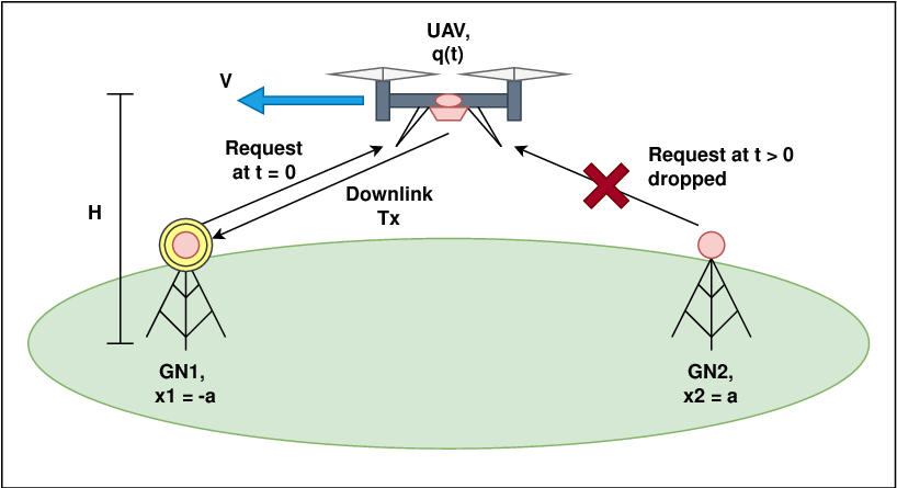
To further motivate the need for this new formulation, consider the scenario depicted in Fig. 1. In this context, the minimum communication delay to serve GN1 is achieved by flying towards it to improve the distance-dependent pathloss. With this design, for a sufficiently large data payload, the UAV will terminate the data transmission hovering above GN1, where channel conditions are most favorable. However, if the UAV is to service a random request generated by GN2 shortly after terminating the transmission to GN1, the delay incurred to serve this second request may be large due to the large distance that separates the UAV from GN2, causing severe pathloss conditions. In other words, under random transmission requests, the greedy delay minimization to serve a certain request may lead the UAV to a position where subsequent random requests cannot be served effectively, yielding poor delay performance in an average long-term sense. This example points to the need to incorporate the random nature of transmission requests in the trajectory design.
To address this question, we consider a scenario in which an UAV is serving two GNs far apart, and receives transmission requests according to a Poisson random process. We formulate the problem as that of designing an adaptive trajectory, so as to minimize the average long-term communication delay incurred to serve the requests of both GNs. We prove that the optimal trajectory in the communication phase operates according to a two-scale optimization: in the outer optimization, the UAV selects a target end position, which optimizes the trade-off between minimizing the delay of the current request, and minimizing the expected average long-term delay; then, in the inner optimization, the UAV travels greedily from the current position to the selected end position while communicating, following the trajectory that greedily minimizes the communication delay for the current request, provided in closed form. We utilize a multi-chain policy iteration algorithm to optimize the selection of the end position in the communication phase and the trajectory during the waiting phase, in which the UAV is not actively servicing downlink transmission requests. Our numerical results reveal that the UAV should always move towards the geometric center of the two GNs during the waiting phase, and that the optimal trajectory during communication phases becomes increasingly independent of the data payload and only determined by system parameters as the data payload value becomes sufficiently large.
The rest of the paper is organized as follows. In Sec. II, we introduce the system model and state the optimization problem; in Sec. III, we formalize the problem as a semi-Markov decision process (SMDP); in Sec. IV, we provide numerical results; lastly, in Sec. V, we conclude the paper with some final remarks.
II System Model and Problem Formulation
II-A System Model
Consider the scenario depicted in Fig. 1, where one rotary-wing UAV services two ground nodes (GNs) with random downlink11 1 This formulation and the analysis can be directly applied to uplink transmissions as well. transmission requests of bits. The two ground units GN1 and GN2 are located at positions and along the -axis, respectively, both at ground level (height ). The UAV moves along the line segment connecting the two GNs, at height from the ground. We let be the UAV’s position along the -axis at time , and we assume that it is either hovering or moving at speed , hence , where denotes derivative of over time.
A base station (BS) connected to the rest of the network is the source of downlink traffic to the two GNs. When a downlink request is generated by a certain GN, the BS transmits the data payload to the UAV, which then relays it to the GN using a decode and forward strategy [7]. We assume that the UAV has a high-capacity link to the BS, hence the communication link between the UAV and the GN constitutes the bottleneck of the overall BS-UAV-GN communication. In the rest of the paper, we thus focus on the UAV-GN communication and neglect the delay over the BS-UAV link. We assume that the UAV transmits at fixed power and that the communication intervals experience LoS links with no probabilistic elements. This is motivated by the fact that UAVs in low-altitude platforms generally tend to have a much higher occurrence of LoS links [8]. We model the instantaneous communication rate between the UAV in position and GN in position as
| (1) |
where is the squared distance between the UAV and GNr, is the channel bandwidth, and is the SNR referenced at meter (see [3]).
When the UAV has no active transmission requests, future requests arrive according to a Poisson process with mean requests/second, independently at each GN. Each request requires the transmission of bits to the corresponding destination. Upon receiving a request from GNr, the UAV enters the communication phase, where it services it by transmitting the bits to GNr; any additional requests received during this communication interval are dropped (see also Fig. 1). After the data transmission is completed, the UAV enters the waiting phase, where it awaits for new requests (with rate for each GN), and the process is repeated indefinitely. During this periodic process of communication and waiting for new requests, the UAV follows a trajectory, part of our design, with the goal to minimize the average long-term communication delay, as discussed next.
II-B Problem Formulation
In this work, we consider the unconstrained delay minimization and neglect the propulsion energy consumption from our problem. In fact, it has been shown that a rotary-wing UAV exhibits comparable energy consumption when either moving or hovering [3]; in the special case when the moving and hovering powers are equal (for instance, based on the model in [3], this occurs at speed m/s), the finite energy in the UAV battery translates into a constraint on the total service time of the UAV, independent of the trajectory followed.
The goal is to define the optimal policy (UAV trajectory) so as to minimize the average communication delay. To this end, let be the delay incurred to complete the transmission of the th request serviced by the UAV. Let be the total number of requests served and completed up to time . Then, we define the expected average delay under a given trajectory policy (to be defined), starting from as22 2 While in practice the operation time of the UAV is constrained by the amount of energy stored in its battery, and the policy should depend on the amount of time left, the asymptotic case is convenient since it gives rise to stationary policies (i.e., time-independent); this is a good approximation when the dynamics of the waiting and communication phases occur at much faster time scales than the total travel time, i.e., when in (2) is large for practical values of the travel time . For perspective, [9] places typical rotary-wing hovering endurance times in the 15-30 minute range.
| (2) |
We then seek to determine to minimize , i.e.,
| (3) |
Note that this is a non-trivial optimization problem. While the minimum delay to serve a request, say from GN1, is achieved by flying towards GN1 at maximum speed to improve the link quality, this strategy may not be optimal in an average delay sense: if the UAV receives a new request from GN2 shortly after completing the request to GN1, the delay to serve this second request may be large due to the large distance that must be covered by the UAV.
II-C Semi-Markov Decision Process (SMDP) formulation
In general, a solution to (3) would involve the optimization of an intractable number of variables over time (i.e., all possible trajectories followed by the UAV at any given time), over a continuous state space (the interval ). Therefore, it is advantageous to approximate the system model through discretization and reformulate (3) as an average-cost SMDP.
We define the state space as , where denotes the request status, i.e., no active request (), or a request is received from GNr (), and
| (4) |
is the set of indices corresponding to discretized positions along the interval . This is a good approximation for sufficiently large , as , making the expected number of requests received over the travel time between two adjacent discretized positions much smaller than one. It is also useful to further partition the state space into waiting states, , and communication states, .
To define this SMDP, we sample the continuous time interval to define a discrete sequence of states with the Markov property. We now define the actions available, the transition probabilities, duration and cost of each state visit.
If the UAV is in state at time , i.e., it is in the discretized position and there are no active requests, then the actions available are , i.e. move right ( to position ), hover (), or move left by one discretized position ( to ). The amount of time required to take this action, i.e., to fly between two adjacent discretized positions, is
| (5) |
The new state is then sampled at time , and is given by . The transition probability from state under action is then given by
| (6) | ||||
depending on whether no request is received during this time interval (, with probability ), or a request is received from GNr (, with probability for each GN).
Upon reaching state with at time , the UAV has received a request to serve bits to GNr. The actions available at this point are all trajectories that start from and allow the UAV to transmit the entire data payload of bits. Assuming a move and transmit strategy (see [3]), the selected trajectory of duration must satisfy
| (7) |
since all bits need to be transmitted during this phase. Under this trajectory, the communication delay is thus . We define the action space in state as the set of all feasible trajectories, , where we have defined as the set of feasible trajectories starting in , ending in , and serving GNr, i.e.,
| (8) |
Upon completing the communication phase, the UAV enters the waiting phase again; the new state is then sampled at time (the amount of time elapsed to complete the selected trajectory), and is given by , corresponding to the position reached at the end of the communication phase. Thus, we have defined the transition probability in the SMDP from state under action as
| (9) |
In other words, the trajectory selection process in the communication phase can be described via a two-scale decision process: 1) given , i.e., the current position of the UAV and the request received from GNr, the UAV first selects some , which defines the target position to be reached at the end of the communication phase; 2) the UAV selects a feasible trajectory from , executes the trajectory while communicating to GNr, and terminates the communication phase in the new position , corresponding to state . After this point, the UAV is in the waiting phase again.
With the states and actions defined, we can define a policy . Specifically, for states , . Likewise, for states , , where (position reached at the end of the communication phase) and (feasible trajectory starting in , ending in , to serve GNr).
The communication delay cost during the waiting phase is zero, i.e. , for all states and actions . When the UAV is in a communicating phase, we denote the communication delay incurred in state under action as . Compactly, we write to denote the delay incurred in state under the action dictated by policy .
With this notation, and having now defined a stationary policy , we can rewrite the average delay in (2) in the context of the SMDP as
| (10) |
where is the indicator function of the event . In fact, the numerator in (2) counts the sample average delay incurred in the communication phases up to slot of the SMDP, whereas the denominator in (2) counts the sample average number of communication slots in the SMDP up to slot . Now, using Little’s Theorem [10], we can rewrite (10) as
| (11) |
where is the steady-state probability in the SMDP of the UAV being in state under policy , and the second equality holds since and for .
III Policy Optimization and Analysis
In this section, we tackle the solution to the optimization problem (3), with given by (II-C). However, (3) cannot be directly solved using dynamic programming techniques, due to the presence of the denominator in (II-C), which depends on the policy selected , hence it affects the optimization. The next lemma demonstrates that the denominator of (II-C) can be expressed as a positive constant, independent from policy and only dependent on system parameters. In doing so, the optimization of only needs to focus on the minimization of , so that (3) can be cast as an average cost per stage problem, solvable with standard dynamic programming techniques.
Lemma 1.
Let and be the steady-state probabilities that the UAV is in the waiting and communication phases, and . We have that
| (12) |
Proof.
Let , , , and be the probabilities of a state request status, , transitioning in the SMDP as , , , and , respectively. Then, (if no request is received, the SMDP remains in the waiting state), , , and (if the SMDP is in the communication state, the next state of the SMDP will be a waiting state, see (9)). Therefore, the steady-state probabilities of being in the waiting and communication states, and , satisfy
whose solution is given as in the statement of the lemma. ∎
When we refer to the denominator of (II-C), it is evident that it is equal to the steady-state probability that the UAV is in a communication state while following policy , . However, with the result of Lemma 1, is simply a positive constant determined by system parameters, yielding
| (13) |
which we now aim to minimize with respect to policy .
As the problem stands now, the communication phase selects an action from , which is a set containing an uncountable number of trajectories. By exploiting the two-scale structure of the problem outlined earlier, we now demonstrate that only a finite set of trajectories from are eligible to be optimal, for each state , hence making the problem a finite state and action SMDP.
III-A Decomposition of Policy
Note from (9) that the transition probability from a communication state under action is only affected by the selection of and not the particular trajectory that leads from to during the communication phase. It follows that the steady-state probability under is only affected by the selection of and not the specific trajectory within .
By establishing this property, we decompose the policy into the waiting policy , which defines the optimal action in state of the waiting phase; the end position policy , which selects the end position with to be reached at the end of the communication phase; and the trajectory policy which, given , selects a trajectory from . Owing to the independence of on the trajectory policy , the delay minimization problem can then be rewritten as
Letting
| (14) |
we can finally write
| (15) |
Note that yields the trajectory that greedily minimizes the communication delay when starting from state , ending in position while serving GNr. This result proves that, for any communication state , there exist only trajectories that are eligible to be optimal, one for each possible ending position . Hence, the problem is finally reduced to that of finding the optimal waiting policy and end position policy , which can be solved efficiently via dynamic programming (Algorithm 1). In the next section, we provide a closed form expression of .
III-B Closed-form Delay Minimizing Trajectory
With the independence of the steady-state probabilities from , we can proceed to solve (14) and then provide the dynamic programming algorithm to solve for and in (15). By definition of in (II-C), we can rewrite as
| (16) |
The minimizer is the trajectory that the UAV should follow when receiving a request from GNr starting in position and ending in position , selected by the end position policy .
In defining the optimal trajectory, the following definitions will be useful. Let be the time needed to fly at maximum speed from to . Along this straight trajectory, let
| (17) |
be the amount of bits transmitted to serve GNr.
Clearly, (), (), and (). The integral can be determined in closed form and is found in [2], for example. We also define the trajectory , as the one in which the UAV starts at position , flies at maximum speed to , hovers at for amount of time, and finally flies at maximum speed from to . Mathematically,
| (18) | ||||
The traffic delivered to GNr when following this trajectory is , with delay . With these definitions, we are now ready to state the main result.
Theorem 1.
Let be the trajectory that minimizes the communication delay . If , then
| (19) |
i.e., the UAV flies at maximum speed from to without interruption; otherwise, if , then
where
| (20) |
i.e., the UAV flies at maximum speed from to , hovers over for amount of time, and then flies to ; finally, if , but , then
where is the unique solution in (if ) or (if ) of ; i.e., the UAV flies at maximum speed towards to the farthest point and then back to , with uniquely defined in such a way as to transmit exactly the data payload upon reaching .
Proof.
Due to space limitations, we provide an outline of the proof. Assume (a similar argument applies to by symmetry). 1) for any trajectory of duration , one can construct another trajectory of same duration , and such that ; such trajectory is obtained by flying at maximum speed towards GN2, possibly hovering on top of GN2 for amount of time (if time allows), and then returning to , yielding , for a proper choice of and such that ; 2) note that the UAV is always closer to GN2 under than it is under , hence it delivers a larger data payload than while incurring the same delay; therefore, is suboptimal; 3) can be further improved by minimizing the delay (by optimizing ), yielding the three cases provided in the statement of the theorem.∎
III-C Multi-chain Policy Iteration (PI) Algorithm
We opt to use a multi-chain PI algorithm to solve (15), as there exist some policies whose induced Markov chain structures are multi-chain. For example, if the waiting policy is , and the end position policy is , then the induced Markov chain has recurrent classes (hence multi-chain). To accommodate this structure, the pseudocode that follows is based upon the multi-chain PI methods of [11] and succinctly describes how to solve for .
In Algorithm 1, we use a vector notation for and , which denote the average delay and relative value for all states, respectively, following the th policy iterate . Likewise, is the vector notation for the delay cost function under policy , supplemented by the optimal minimized communication delays described by (14) and (III-B), and is the transition matrix under policy .
IV Numerical Results
We use the following system parameters, unless specified otherwise: number of states ; channel bandwidth ; -meter reference SNR ; UAV height ; GN locations , ; UAV speed ; and request arrival rate requests/second.
We vary the data payload across a range of values and find numerically that, regardless, the optimal policy in the waiting phase optimized with Algorithm 1 is
| (21) |
In other words, in the waiting phase it is optimal for the UAV to move towards the geometric center of the two GNs along the line segment connecting the two. Intuitively, the UAV can more readily service a request that is originated equally likely from GN1 or GN2, if it is located in the geometric center when the request arrives, since the UAV is equally distant from both GNs, and can thus serve them equally well.

In Fig. 2, we plot the optimal end position policy for different data payload values.33 3 We omit the figure for states , due to the inherent symmetry of the problem. Specifically, if the optimal end point is observed, then is also observed. We note that, for large data payload values , the optimal end position in the communication phase becomes independent of the initial position (in this case, , irrespective of for ). In fact, for large data payload , the UAV hovers over the receiver for a significant amount of time during the communication phase (case in Theorem 1), hence the final part of the trajectory from to the selected end position becomes irrespective of the actual data payload value. However, does depend on other system parameters, such as the request rate and UAV height , as seen in Fig. 3. Interestingly, as the request rate increases (the inter-arrival request time decreases) the end position is closer to the geometric center (i.e., farther away from the receiver); this is because requests arrive more often, hence it is desirable for the UAV to terminate the communication phase closer to the center, in order to more readily serve future requests.

Next, we illustrate how the optimal expected average delay , across the same set of data payload values, fares against a heuristic policy which operates as follows: in the waiting phase, hover in the current position; in the data communication phase, greedily minimize the delay by flying at maximum speed towards the receiver until completion. The comparison between the optimal policy and the heuristic policy is shown for the span of data payload values in Fig. 4. Note that the slope of the line for both the optimal and heuristic policies saturates to . In fact, when , the UAV spends most of the communication time hovering above the receiver (case in Theorem 1), hence in (15), yielding
Overall, the heuristic scheme performs worse, roughly by seconds for large . In fact, when hovering during the waiting phase instead of moving towards the center, the UAV incurs a larger delay to serve a request generated by the more distant GN, due to the longer distance that needs to be covered.
V Conclusions
In this paper, we studied the trajectory optimization problem of one UAV servicing random downlink transmission requests by two GNs, to minimize the expected communication delay. We formulated the problem as an SMDP, and exploited the structure of the problem to simplify the trajectory design in the communication phase. We showed that the problem exhibits an interesting two-scale structure in the optimal trajectory design, and can be solved efficiently via dynamic programming. Numerical evaluations demonstrate consistent improvements in the delay performance over a sensible heuristic, for a variety of data payload values.

References
- [1] Q. Wu, L. Liu, and R. Zhang, “Fundamental Trade-offs in Communication and Trajectory Design for UAV-Enabled Wireless Network,” IEEE Wireless Communications, vol. 26, pp. 36–44, 02 2019.
- [2] Y. Zeng and R. Zhang, “Energy-Efficient UAV Communication With Trajectory Optimization,” IEEE Transactions on Wireless Communications, vol. 16, no. 6, pp. 3747–3760, June 2017.
- [3] Y. Zeng, J. Xu, and R. Zhang, “Energy Minimization for Wireless Communication With Rotary-Wing UAV,” IEEE Transactions on Wireless Communications, vol. 18, no. 4, pp. 2329–2345, April 2019.
- [4] H. Bayerlein, P. De Kerret, and D. Gesbert, “Trajectory Optimization for Autonomous Flying Base Station via Reinforcement Learning,” in IEEE 19th International Workshop on Signal Processing Advances in Wireless Communications (SPAWC), June 2018, pp. 1–5.
- [5] M. Mozaffari, W. Saad, M. Bennis, and M. Debbah, “Optimal transport theory for power-efficient deployment of unmanned aerial vehicles,” in 2016 IEEE International Conference on Communications (ICC), May 2016, pp. 1–6.
- [6] J. Chen and D. Gesbert, “Optimal positioning of flying relays for wireless networks: A LOS map approach,” in 2017 IEEE International Conference on Communications (ICC), May 2017, pp. 1–6.
- [7] T. Cover and A. E. Gamal, “Capacity theorems for the relay channel,” IEEE Transactions on Information Theory, vol. 25, no. 5, pp. 572–584, Sep. 1979.
- [8] Y. Zeng, R. Zhang, and T. J. Lim, “Wireless communications with unmanned aerial vehicles: opportunities and challenges,” IEEE Communications Magazine, vol. 54, no. 5, pp. 36–42, May 2016.
- [9] M. Gatti, F. Giulietti, and M. Turci, “Maximum endurance for battery-powered rotary-wing aircraft,” Aerospace Science and Technology, vol. 45, 09 2015.
- [10] J. D. C. Little and S. Graves, Little’s Law, 07 2008, pp. 81–100.
- [11] M. L. Puterman, Markov decision processes: discrete stochastic dynamic programming. John Wiley & Sons, 2014.