Stationary Markovian Arrival Processes,
Results and Open Problems
Abstract
We consider two classes of irreducible Markovian arrival processes specified by the matrices and . The Markov Modulated Poison Process (MMPP) and the Markovian Switched Poison Process (MSPP). The former exhibits a diagonal while the latter exhibits a diagonal . For these two classes, we consider the following statements: (I) Overdispersion of the counts process. (II) A non-increasing hazard rate of the stationary inter-event time. (III) The squared coefficient of variation of the event stationary process is greater or equal to unity. (IV) A stochastic order showing that the time stationary inter-arrival time dominates the event-stationary time. For general MSPPs and two-state MMPPs, we show that (I)-(IV) hold. Then for general MMPPs, it is easy to establish (I), while (II) is false due to a counter-example of Miklos Telek and Illes Horvath. For general simple point processes, (III) follows from (IV). For MMPPs we conjecture and numerically test that (IV) and thus (III) hold. Importantly, modeling folklore has often treated MMPPs as “bursty” and implicitly assumed that (III) holds. However, this is still an open question.
Keywords: Markovian Arrival Processes (MAPs), Markov Modulated Poisson Process (MMPP), Markov switched Poisson process, overdispersion, hazard rate, squared coefficient of variation, inter-event times, stationary process.
1 Introduction
Point processes on the line, generated by transitions of Continuous Time Markov Chains (CTMCs) have been studied intensely by the applied probability community over the past few decades under the umbrella of Matrix Analytic Methods (MAM), see e.g. [16]. These have been applied to teletraffic [1], business networks [14], social operations research [25], and biological systems [20]. The typical model referred to as the Markovian Arrival Process (MAP) is comprised of a finite state irreducible CTMC which generates events at selected instances of state change and/or according to Poisson processes modulated by the CTMC. MAPs have been shown to be dense in the class of point processes so that they can essentially approximate any point process, [5]. Yet at the same time, they are analytically tractable and may often be incorporated effectively within more complex stochastic models [19].
In general, treating point processes as stationary often yields a useful mathematical perspective which matches scenarios when there is no known dependence on time. In describing a point process we use to denote the number of events during and further use the sequence to denote the sequence of inter-event times. Two notions of stationarity are useful in this respect. Roughly, a point process is time-stationary if the distribution of the number of events within a given interval does not depend on the location of the interval; that is if is distributed as for any non-negative and . A point process is event-stationary if the joint distribution of is the same as that of for any integer sequence of indices and any integer shift . For a given model of a point process, one may often consider either the event-stationary or the time-stationary case. The probability laws of both cases agree in the case of the Poisson process. However, this is not true in general. For MAPs, time-stationarity and event-stationarity are easily characterized by the initial distribution of the background CTMC. Starting it at its stationary distribution yields time-stationarity and starting at the stationary distribution of the embedded Markov chain (jump chain) yields event-stationarity.
A common way to parameterize MAPs is by considering the generator, , of an irreducible finite state CTMC and setting . Roughly speaking, the matrix determines state transitions without event counts and the matrix determines event counts. Such parameterization hints at considering two special cases: Markov Modulated Poisson Processes (MMPP) arising from a diagonal matrix , and Markovian Switched Poisson Processes (MSPP) arising from a diagonal matrix .
MMPPs are a widely used class of processes in modelling and are a typical example of a Cox process, also known as a doubly stochastic Poisson process, [11] and [23]. For a detailed outline of a variety of classic MMPP results, see [10] and references therein. MSPPs were introduced in [9] and to date, have not been as popular for modeling. However, the duality of diagonal vs. diagonal motivates us to consider and contrast both these processes. We also note that hyper-exponential renewal processes are special cases of MSPPs as well as Markovian Transition Counting Processes (as introduced in [3]).
Our focus in this paper is on second order properties of MMPPs and MSPPs and related traits. Consider the squared coefficient of variation and the limiting index of dispersion of counts given by,
| (1) |
where is the time of the first event, taken from the event stationary version. Modelling folklore of MMPP sometimes assumes that . This is perhaps due to the fact that is straightforward to verify and the similarity between these measures (for example for a renewal process, ). However, as we highlight in this paper, establishing such “burstiness” properties is not straightforward.
A related property is having exhibit Decreasing Hazard Rate (DHR), where for a random variable with PDF and CDF the hazard rate is,
A further related property is the stochastic order, where is the first event time in the time-stationary version. We denote the properties as follows:
-
(I) .
-
(II) exhibits DHR.
-
(III) .
-
(IV) The stochastic order .
All these properties are related and in this paper we highlight relationships between (I), (II), (III) and (IV) and establish the following: For MSPPs and MMPPs of order we show that (I)–(IV) holds. For general MMPPs it is known that (I) holds however, a counter-example of Miklos Telek and Illes Horvath shows that (II) does not hold and we conjecture (and numerically test) that (III) and (IV) holds.
Our interest in this class of problems stemmed from relationships between different types of MAPs as in [24] and [3]. Once it became evident that for MMPPs is an open problem even though it is acknowledged as a modeling fact in folklore, we searched for alternative proof avenues. This led to the stochastic order in (IV) as well as to considering DHR properties (the latter via communication with Miklos Telek and Illes Horvaths).
2 Preliminaries
Consider first properties (I)–(IV) and their relationships. With an aim of establishing property (III), , there are several possible avenues based on properties (I), (II) and (IV). We now explain these relationships.
Using property (I):
First, from the theory of simple point processes on the line, note the relationship between and :
| (2) |
However, the autocorrelation structure is typically intractable and hence does not yield results. If we were focusing on a renewal process where and are independent for then this immediately shows that . Our focus is broader and hence property (I) indicating that does not appear to be of use.
Using property (II):
An alternative way is to consider property (II) and use the fact that for any DHR random variable we have (see [22]). Hence if property (II) holds then (III) holds.
Using property (IV):
We have the following Lemma, implying that (III) is a consequence of the stochastic order (IV).
Lemma 2.1.
Consider a simple non-transient point process on the line, and let , represent the first inter-event time in the time-stationary case and event-stationary case respectively. Then if and only if .
Proof.
From point process theory (see for example, Eq. (3.4.17) of [8]), it holds
where,
Now,
and we obtain the result. ∎
MAPs:
We now describe Markovian Arrival Process (MAPs). A MAP of order (MAPp) is generated by a two-dimensional Markov process on state space . The counting process counts the number of “events” in with . The phase process is an irreducible CTMC with state space , initial distribution and generator matrix . A MAP is characterized by parameters , where the matrix has negative diagonal elements and non-negative off-diagonal elements and records the rates of phase transitions which are not associated with an event. The matrix has non-negative elements and describes the changes of the phase process with an event (increase of by 1). Moreover, we have . More details are in [4] (Chapter XI) and [12] (Chapter 2).
MAPs are attractive due to the tractability of many of their properties, including distribution functions, generating functions, and moments of both and the sequence of inter-event times . Since is assumed irreducible and finite, it has a unique stationary distribution satisfying , . Note that from we have . Of further interest is the embedded discrete-time Markov chain with irreducible stochastic matrix and stationary distribution , where and .
Observe the relation between the stationary distributions and :
| (3) |
where .
The following known proposition, as distilled from the literature (see for example [4], Chapter XI) provides the key results of MAPs that we use in this paper. It shows that is a Phase Type (PH) random variable with parameters for the initial distribution of the phase and for the sub-generator matrix. It further shows that the initial distribution of the phase process may render the MAP as time stationary or event stationary.
Proposition 2.2.
Consider a MAP with parameters (,,), then
| (4) |
Further, if then the MAP is time-stationary and if it is event stationary, where and are associated stationary distributions.
Note that for such a random variable the density and the hazard rate , are respectively,
Further, as may be used for showing DHR, the derivative of the hazard rate is,
| (5) |
We now describe second-order properties associated with each case.
Event-Stationary Case:
The MAP is event-stationary11 1 Sometimes an event-stationary MAP is referred to as an interval-stationary MAP, see for instance [10]. if . In this case, the (generic) inter-event time is phase-type distributed, and thus has -th moment:
with the first and second moments (here represented in terms of and ):
The squared coefficient of variation (SCV) of events (intervals) has a simple formula:
| (6) |
Time-Stationary Case:
A MAP with parameters is time-stationary if . In the time-stationary case (), we have (see [4]):
| (7) | ||||
| (8) |
where is the deviation matrix associated with defined by the following formula.
| (9) |
Note that in some sources, for instance [4] and [17], the variance formula (8) is presented in terms of the matrix . The relation between these two matrices is , see [7].
MMPP:
A MAP with a diagonal matrix is an MMPP. MMPPs correspond to doubly-stochastic Poisson processes (also known as Cox processes) where the modulating process is driven by a CTMC. MMPPs have been used extensively in stochastic modelling and analysis, see for example [10]. The parameters of an MMPPp are , where for , and . Here, is the generator matrix of a CTMC. For MMPPs, (7) and (8) can be simplified by using the following relations:
MSPP:
A MAP with a diagonal matrix is is an MSPP. For MSPPp events switch between Poisson processes with rates , where each switch also incurs an event. Here as in MMPPs we denote the diagonal elements of via . However, unlike MMPPs, (irreducible) MSPPs don’t have a diagonal . We also remark that the modulation in the MSPP is of a discrete nature and it occurs at certain event epochs of the counting process, whereas the modulation of the MMPP is performed at epochs without events. See [2] and [12].
As our research attempts have shown, analyzing MSPPs is considerably easier than MMPPs, because a diagonal is much easier to handle than a non-diagonal and in an (irreducible) MMPP, must be non-diagonal.
Properties (I)-(IV) for MAPs:
Using the results above, for any irreducible MAP with matrices and we have that the main properties (I)-(IV) of this paper can be formulated as follows:
| (11) | ||||
| (12) | ||||
| (13) | ||||
| (14) |
3 Main Results
We now present results for MSPP and MMPP2 for properties (I)-(IV) as presented in the introduction. Establishing property (I), is not a difficult task for both MMPPs and MSPPs:
Proposition 3.1.
MMPP and MSPP processes have .
Proof.
This is a well-known result that for all doubly stochastic Poisson processes (Cox processes), . So, we have the proof for an MMPP, for instance see Chapter 6 of [15].
It isn’t difficult to show that property (II), DHR holds for MSPP:
Proposition 3.2.
For an MSPP the hazard rate of the stationary inter-event time is non-increasing.
Proof.
Denote the diagonal matrix with and the positive elements of the column vector with . So, Eq. (12) can be written element-wise as:
| (16) |
Denoting and assuming results in:
The above expression can be viewed as the minus variance of a random variable that takes values with probability . Therefore, we have (12).
∎
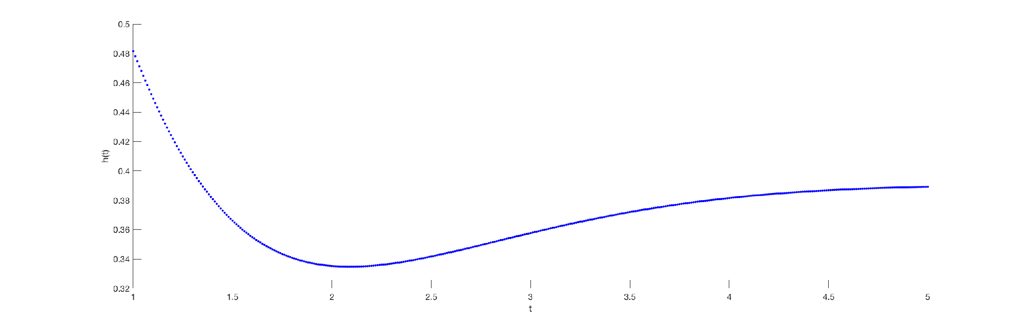
However, somewhat surprisingly, MMPPs don’t necessarily possess DHR. An exception is MMPP2 as shown in Proposition 3.6. However for higher order MMPPs DHR doesn’t always hold. The gist of the following example was communicated to us by Milkos Telek and Illes Horvath. Set
| (17) |
As shown in Figure 1, the hazard rate function for an MMPP with the above matrices is not monotone. Hence at least for general MMPPs, trying to show (III), , via hazard rates is not a viable avenue.
Since hazards rates don’t appear to be a viable paths for establishing (III) for MMPPs, an alternative may be to consider the stochastic order (IV). Starting with MSPPs, we see that this property holds.
Proposition 3.3.
For an MSPP .
Proof.
Using (14), the claim is,
| (18) |
Without loss of generality we assume that there is an order (with for some ) for diagonal elements of matrix . There is a possibility that for , , and , however, in the rest of the proof, we assume that , meaning that all are strictly positive. Adapting to the case of is straightforward.
Now, is a non-increasing sequence and therefore in the sequence when an element is negative, all the elements for are negative. Moreover, both and are probability vectors, so . Therefore, at least the first element in the sequence is positive. Hence, there exists an index such that for is non-negative and for is negative. Therefore, we have:
Assume: :
| (19) |
Then, since , we have . Now from (19) we can conclude that:
Using the fact that , results in:
which is not true. Consequently, the assumption is not true and hence (14) holds.
∎
Corollary 3.4.
For an MSPP .
In fact, for MSPPs this is an easy result and it can also be proved independently by using the Cauchy-Schwarz inequality. Further, we can find an upper bound:
Proposition 3.5.
An MSPP with diagonal matrix for satisfies
where and .
Proof.
From Eq. (6), we have . For , we have and so,
On the other hand, from the Cauchy-Schwarz inequality and the Kantorovich’s Inequality (see [21]), we have:
Combination of the above two equations results in:
which completes the proof.
∎
However, for MMPPs while we believe the result is true (see numerical evidence in the next section) we don’t have a general proof for properties (III) or (IV). Still, for two state MMPPs (MMPP2) things are easier and we are able to show that all properties (I)-(IV) hold:
Proposition 3.6.
For a two-state MMPP2, and , is DHR and the stochastic order holds.
Proof.
Consider an MMPP2 with parameters
Then, . As in [13], evaluation of the transient deviation matrix through (for e.g.) Laplace transform inversion yields:
Therefore from (1), we have
Further, explicit computation yields,
Thus it is evident that the MMPP2 has as long as and when .
For DHR and the stochastic order, first we note that for an MMPP2 with the above parameters, . By setting and , after some simplification, Eq. (12) is given by:
which is strictly negative for and is zero for . For the stochastic order, from Eq. (14), we have:
which is strictly positive for and is zero for .
∎
4 Conjectures for MMPP
We embarked on this research due to the folklore assumption that for MMPP, (III). Initially we believed that it is easy to verify, however to date there isn’t a known proof for an arbitrary irreducible MMPP. Still, we conjecture that both (III) and (IV) hold for MMPPs:
Conjecture 4.1.
For an irreducible MMPP, .
Conjecture 4.2.
For an irreducible MMPP, .
In an attempt to disprove these conjectures or alternatively gain confidence in their validity, we carried out an extensive numerical experiment. Our experiment works by generating random instances of MMPPs . Each instance is generated by first generating a matrix with uniform off-diagonal entries and diagonal entries that ensure row sums are . We then generate a matrix with diagonal elements that are exponentially distributed with rate . Such a pair then implies and . For each such MMPP we calculate as in (13) and as in (14), where we take . We then ensure that both of these quantities are non-negative.
We repeated this experiment for random MMPP instances of orders and . In all cases the calculated quantities were greater that . Note that in certain cases, the quantity associated with (IV) was negative and lying in the range . We attribute this to numerical error stemming from the calculation of the matrix exponential . We ran our experiments with the Julia programming language, V1.0. The calculation time was about 1.5 hours.
This provides some evidence for the validity of Conjectures 1 and 2, although it is clearly not a proof. Further, we note that it is possible that some extreme cases exist that are not likely to come up by uniformly and randomly generating entries of . For example the cyclic matrix in (17). For this we have also considered random cyclic matrices with non-zero entries similar to (17). We generated such (order ) examples and all agreed with (III) and (IV).
5 Conclusion
We have highlighted various related properties for point processes on the line and MAPs exhibiting diagonal matrices ( or ) in particular. Showing that for MMPP and establishing the stochastic order remains an open problem. We have shown this for MMPPs of order and using a similar technique to our MSPP proof, we can also show it for MMPPs with symmetric matrices. However for general MMPPs this remains an open problem.
We note, that stepping outside of the matrix analytic paradigm and considering general Cox processes is also an option. In fact, since any Cox process can be approximated by an MMPP, we believe that versions of conjectures and also hold for Cox processes under suitable regularity conditions.
There is also a related branch of questions dealing with characterizing the Poisson process via and considering when an MMPP is Poisson. For example, for the general class of MAPs, the authors of [6] provide a condition for determining if a given MAP is Poisson. It is not hard to construct a MAP with that is not Poisson. But, we believe that all MMPPs with are Poisson. Yet, we don’t have a proof. Further, we believe that for an MMPP, if then all are equal (the converse is trivially true). We don’t have a proof of this either. Related questions also hold for the more general Cox processes.
We also note that the MSPP class of process that we considered generalized hyper-exponential renewal processes as well as a class of processes called Markovian Transition Counting Processes (MTCP) as in [3].
Acknowledgement
Azam Asanjarani’s research is supported by the Australian Research Council Centre of Excellence for the Mathematical and Statistical Frontiers (ACEMS). Yoni Nazarathy is supported by Australian Research Council Grant DP180101602. We thank Soren Asmussen, Qi-Ming He, Illes Horvath, Peter Taylor and Miklos Telek for useful discussions and insights related to this problem.
References
- [1] Akar N., Oguz N.C., and Sohraby K. Matrix-geometric solutions of M/G/1-type Markov chains: a unifying generalized state-space approach. Selected Areas in Communications, IEEE Journal on, 16(5):626–639 (1998)
- [2] Artalejo J.R., Gómez-Corral A., and He Q.M. Markovian arrivals in stochastic modelling: a survey and some new results. SORT, 34(2):101–144 (2010)
- [3] Asanjarani A. and Nazarathy Y. A queueing approximation of MMPP/PH/1. Queueing Theory and Network Applications, pages 41–51, Springer (2016)
- [4] Asmussen S. Applied Probability and Queues, volume 51. Springer (2003)
- [5] Asmussen S. and Koole G. Marked point processes as limits of Markovian arrival streams. Journal of Applied Probability, 30:365–365 (1993)
- [6] Bean N.G. and Green D.A. When is a MAP Poisson? Mathematical and Computer Modelling, 31(10-12):31–46 (2000)
- [7] Coolen-Schrijner P. and Van Doorn E.A. The deviation matrix of a continuous-time Markov chain. Probability in the Engineering and Informational Sciences, 16(03):351–366 (2002)
- [8] Daley D. and Vere-Jones D. An introduction to the theory of point processes: volume II: general theory and structure. Springer Science & Business Media (2007)
- [9] Liu D. and Neuts M.F. Counter-examples involving Markovian arrival processes. Stochastic Models, 7(3):499–509 (1991)
- [10] Fischer W. and Meier-Hellstern K. The Markov-modulated Poisson process (MMPP) cookbook. Performance Evaluation, 18(2):149–171 (1993)
- [11] Grandel J. Doubly stochastic Poisson processes. volume 529, Springer (2006)
- [12] He Q.M. Fundamentals of Matrix-Analytic Methods. Springer (2014)
- [13] Heffes H. and Lucantoni D. A Markov modulated characterization of packetized voice and data traffic and related statistical multiplexer performance. Selected Areas in Communications, IEEE Journal on, 4(6):856–868 (1986)
- [14] Herbertsson A. and Rootzén H. Pricing kth-to-default swaps under default contagion: the matrix-analytic approach. Available at SSRN 962381 (2007)
- [15] Kingman J.F.C. Poisson Processes. Wiley Online Library (1993)
- [16] Latouche G. and Ramaswami V. Introduction to Matrix Analytic Methods in Stochastic Modeling, volume 5. Siam (1999)
- [17] Narayana S. and Neuts M.F. The first two moment matrices of the counts for the Markovian arrival process. Communications in Statistics. Stochastic Models, 8(3):459–477 (1992)
- [18] Nazarathy Y. and Weiss G. The asymptotic variance rate of the output process of finite capacity birth-death queues. Queueing Systems, 59(2):135–156 (2008)
- [19] Neuts M.F. A versatile Markovian point process. Journal of Applied Probability, pages 764–779 (1979)
- [20] Olsson F. and Hössjer O. Equilibrium distributions and simulation methods for age structured populations. Mathematical Biosciences, 268:45–51 (2015)
- [21] Steele J.M. The Cauchy-Schwarz Master Class: An Introduction to the Art of Mathematical Inequalities. Cambridge University Press (2004)
- [22] Stoyan D. and Daley D.J. Comparison Methods for Queues and Other Stochastic Models. JOHN WILEY & SONS, INC., 605 THIRD AVE., NEW YORK, NY 10158, USA (1983)
- [23] Tang, L.C. Markov-modulated processes and semiregenerative phenomena, World Scientific (2009)
- [24] Nazarathy Y. and Weiss G. The asymptotic variance rate of the output process of finite capacity birth-death queues. Queueing Systems, 59 (2), p. 135. Springer (2008)
- [25] Xing Y., Li L., Bi Z., Wilamowska-Korsak M., and Zhang L. Operations research (OR) in service industries: a comprehensive review. Systems Research and Behavioral Science, 30(3):300–353 (2013)