Reconstruction of domains with algebraic boundaries from generalized polarization tensors Thanks: This work was supported in part by the grant ANR-17-CE40-0029 of the French National Research Agency ANR (project MultiOnde), the LabEx PERSYVAL-Lab (ANR-11-LABX- 0025-01), and the Swiss National Science Foundation grant number 200021–172483.

Habib Ammari Address: Habib Ammari, Department of Mathematics, ETH Zürich, Rämistrasse 101, 8092 Zürich, Switzerland Email address: habib.ammari@math.ethz.ch , Mihai Putinar Address: Mihai Putinar, Department of Mathematics, University of California at Santa Barbara, Santa Barbara, CA 93106-3080, USA, and School of Mathematics & Statistics, Newcastle University Newcastle upon Tyne, NE1 7RU, United Kingdom Email address: mputinar@math.ucsb.edu , Andries Steenkamp Address: Andries Steenkamp, Department of Mathematics, ETH Zürich, Rämistrasse 101, 8092 Zürich, Switzerland Email address: andriess@student.ethz.ch and Faouzi Triki Address: Faouzi Triki, Laboratoire Jean Kuntzmann, UMR CNRS 5224, Université Grenoble-Alpes, 700 Avenue Centrale, 38401 Saint-Martin-d’Hères, France Email address: faouzi.triki@univ-grenoble-alpes.fr

Date: August 11, 2026

Abstract.

This paper aims at showing the stability of the recovery of a smooth planar domain with a real algebraic boundary from a finite number of its generalized polarization tensors. It is a follow-up of the work [H. Ammari et al., Math. Annalen, 2018], where it is proved that the minimal polynomial with real coefficients vanishing on the boundary can be identified as the generator of a one dimensional kernel of a matrix whose entries are obtained from a finite number of generalized polarization tensors. The recovery procedure is implemented without any assumption on the regularity of the domain to be reconstructed and its performance and limitations are illustrated.

Key words and phrases:

inverse problems, generalized polarization tensors, algebraic domains, shape classification

1991 Mathematics Subject Classification

Primary: 35R30, 35C20.

1. Introduction

Let $D$ be a bounded connected Lipschitz domain in ${\mathbf{R}}^{2}$ , and assume that its boundary $\partial D$ contains the origin. Let $\Upsilon$ be the conductivity distribution in ${\mathbf{R}}^{2}$ given by

\displaystyle\Upsilon=k\chi(D)+\chi({\mathbf{R}}^{2}\setminus\overline{D}),

where $\chi$ denotes the indicator function, and $k$ is a fixed constant in $(0,1)\cup(1,+\infty)$ . Let $u_{0}(x)=\frac{1}{2\pi}\ln|x|$ , be the fundamental solution to the Laplacian in ${\mathbf{R}}^{2}$ . For a given position $z$ in ${\mathbf{R}}^{2}$ , we consider the following conductivity equation

\displaystyle\left\{\begin{array}[]{ll}\nabla\cdot\Upsilon\nabla u(x,z)=\delta_{z}(x)&\mbox{in }{\mathbf{R}}^{2},\\ u(x,z)-u_{0}(x,z)=O(|x|^{-1})&\mbox{as }|x|\to\infty,\end{array}\right.

where $\delta_{z}$ is the Dirac function at $z$ and $u_{0}(x,z):=u_{0}(x-z)$ . The system (1) has a unique solution $u$ which is the total voltage potential generated by the point source placed at $z$ [7]. The function $-\nabla u_{0}(x,z)$ represents the background electric field while $u(x,z)-u_{0}(x,z)$ is the perturbation of the voltage potential due to presence of the inclusion $D$ . Then, the far-field perturbation of the voltage potential due to the presence of $D$ is given by [7]

(2)

\displaystyle u(x,z)-u_{0}(x,z)=\sum_{|\alpha|,|\beta|=1}^{\infty}\frac{(-1)^{|\alpha|+|\beta|}}{\alpha!\beta!}\partial^{\alpha}u_{0}(x)\mathbf{M}_{\alpha\beta}\partial^{\beta}u_{0}(z)\qquad\textrm{as }|x|\rightarrow+\infty,

where and throughout this paper, we use the conventional notation:

x^{\alpha}=x_{1}^{\alpha_{1}}x_{2}^{\alpha_{2}},\;\;\alpha=(\alpha_{1},\alpha_{2})\in\mathbf{N}^{2},\;\textrm{ and}\;|\alpha|=\alpha_{1}+\alpha_{2}.

We also use the graded lexicographic order: $\alpha,\,\beta\in\mathbf{N}^{2}$ verifies $\alpha\leq\beta$ if $|\alpha|<|\beta|$ , or, if $|\alpha|=|\beta|$ , then $\alpha_{1}\leq\beta_{1}$ or $\alpha_{1}=\beta_{1}$ and $\alpha_{2}\leq\beta_{2}.$

The quantities $\mathbf{M}_{\alpha\beta}$ that appear naturally in the multi-polar asymptotic expansion (2), are called Generalized Polarization Tensors (GPTs). We emphasize that GPTs are not dependent on the positions $x$ and $z$ . In fact they only depend on the inclusion $D$ and the conductivity ratio $1/k$ or conductivity contrast $\lambda:=\frac{k+1}{2(k-1)}$ . For a fixed contrast $\lambda$ , the GPTs are indeed geometric quantities associated with the shape of the domain $D$ such as eigenvalues, capacities, and moments. The notion of GPTs has been used in diverse fields of academic research as well as of engineering applications such as the theories of composites, inverse problems, bio-medical imaging, bio-sensing, nano-sensing, and electro-sensing [5, 9, 11, 12, 13, 10, 15, 26].

From the asymptotic expansion (2), we deduce that the knowledge of all the GPTs is equivalent to knowing the far-field responses of the inclusion for all harmonic excitations. It is well known that in that case the inverse problem of recovering $(\lambda,D)$ has a unique solution [6], and a number of algorithms have been proposed for its numerical treatment [7, 3, 4, 8]. However, in applications, the GPTs are usually only measured with finite accuracy and only a finite number of them can be determined from noisy data. Hence, studying the well-posedness of the inverse problem when only a finite number of GPTs are available is of importance.

The purpose of this paper is to evaluate how much information one can get from the knowledge of a finite number of these GPTs. Precisely, assuming that the domain has an algebraic boundary, we are interested in the inverse problem of recovering its position, its shape and the contrast for given a finite number of its GPTs. Recently the uniqueness to this inverse problem was established by the same authors [1]. Our goal in the present paper is twofold: (i) to quantify the stability of the inversion and (ii) to implement the inversion procedure and apply it to much more general cases than those discussed in [1]. In particular, we show here how to recover the true domain (with possibly nonsmooth boundary) from the recovered polynomial level set even in the case where several candidate domains have the same polynomial level set. In doing so, we resolve key numerical issues which include handling of bifurcation points, segmentation points, and arc sets. It is worth emphasizing that the stability estimates proved in this paper holds for algebraic domains with smooth boundaries. Their generalization to the nonsmooth case is technically quite challenging.

The paper is organized as follows. In Section 2, we introduce the class under consideration of domains with algebraic boundaries. Stability issues are studied in Section 3. The main stability estimates are given in Theorem 3.2. Section 4 is devoted to the presentation of our new numerical algorithm which is designed to recover algebraic domains from finite numbers of their associated GPTs. It is worth mentioning that based on the density with respect to Hausdorff distance of algebraic domains among all bounded domains, the proposed algorithm can be extended via approximation beyond its natural context. This observation has already turned algebraic curves into an efficient tool for describing shapes and reconstructing them from their associated moments [19, 20, 21, 22, 23, 25].

2. Real algebraic domains

In this section, we introduce the class of bounded open subsets in ${\bf R}^{2}$ with real algebraic boundaries. We recall the following definition.

Definition 2.1.

An open set $G$ in ${\mathbf{R}}^{2}$ is called real algebraic (or simply algebraic) if there exists a finite number of real coefficient polynomials $g_{i}(x),i=1,\cdots,m$ , such that

\displaystyle\partial G\subset V:=\{x\in{\mathbf{R}}^{2}\;:g_{1}(x)=\cdots=g_{m}(x)=0\}.

The ellipse is a simple example of an algebraic domain, since its general boundary coincides with the zero set of the quadratic polynomial function

g(x)=\sum_{|\alpha|\leq 2}g_{\alpha}x^{\alpha}

for given real coefficients $(g_{\alpha})_{{|\alpha|\leq 2}}$ and proper signs in the top degree part.

We further denote by $\mathcal{G}$ the collection of bounded algebraic domains. It is well-known that the differential structure of the boundary $\partial G$ consists of algebraic arcs joining finitely many singular points, see for instance [16].

As mentioned in [1], since the connectedness of the respective sets is not accessible by the linear algebra tools we developed for reconstructing an algebraic domain from a finite number of its generalized polarization tensors, we drop such a constraint here. Nevertheless, we call "domains" all elements $G\in\mathcal{G}$ .

Following [23] we consider a particular class of algebraic domains which are better adapted to the uniqueness and stability of our inverse shape problem. Let

(3)

\displaystyle\mathcal{G}^{*}:=\left\{G\in\mathcal{G}:G=\textrm{int}\,\overline{G}\right\}.

An element of $\mathcal{G}^{\ast}$ is called an admissible domain, although it may not be connected.

The assumption that $G=\textrm{int}\,\overline{G}$ implies that $G$ contains no slits or $\partial G$ does not have isolated points. If $G\in\mathcal{G}^{*}$ , the algebraic dimension of $\partial G$ is one, and the ideal associated to it is principal. To be more precise, $\partial G$ is contained in a finite union of irreducible algebraic sets $X_{j},\ j\in J,$ of dimension one each. The reduced ideal associated to every $X_{j}$ is principal:

I(X_{j})=(P_{j}),\ \ \ j\in J;

see, for instance, [14, Theorem 4.5.1]. We assume that each $P_{j}$ is indefinite, i.e., it changes sign when crossing $X_{j}$ . Therefore, one can consider the polynomial $g=\prod_{j\in J}P_{j}$ , vanishing of the first-order on $\partial G$ , that is $|\nabla g|\not=0$ on the regular locus of $\partial G$ . According to the real version of Study’s lemma (cf. [16, Theorem 12]) every polynomial vanishing on $\partial G$ is a multiple of $g$ , that is $I(\partial G)=(g)$ . We define the degree of $\partial G$ as the degree of the generator $g$ of the ideal $I(\partial G)$ . For a thorough discussion of the reduced ideal of a real algebraic surface in ${\mathbf{R}}^{d}$ , we refer the reader to [17].

Throughout this paper, we denote by $g(x)$ the single polynomial vanishing on $\partial G$ which is the generator of $I(\partial G)$ and satisfying the following normalization condition $g_{\alpha^{*}}=1$ , where $\alpha^{*}=\max_{g_{\alpha}\not=0}\alpha$ . We further assume that $G\in\mathcal{G}^{*}$ .

3. Uniqueness and stability estimates

In this section, we first recall the uniqueness result obtained in [1] and then derive stability estimates for the inversion procedure for smooth algebraic domains.

3.1. Uniqueness

Let ${\mathbf{R}}[x]$ be the ring of polynomials in the variables $x=(x_{1},x_{2})$ and let ${\mathbf{R}}_{n}[x]$ be the vector space of polynomials of degree at most $n$ (whose dimension is $r_{n}=(n+1)(n+2)/2$ ). Any polynomial function $p(x)\in{\mathbf{R}}_{n}[x]$ has a unique expansion in the canonical basis $x^{\alpha},|\alpha|\leq n$ of ${\mathbf{R}}_{n}[x]$ , that is,

\displaystyle p(x)=\sum_{|\alpha|\leq n}p_{\alpha}x^{\alpha},

for some vector coefficients ${\bf p}=(p_{\alpha})\in{\mathbf{R}}_{r_{n}}$ . The following results are established in [1].

Theorem 3.1.

Let $G\in\mathcal{G}^{*}$ with $\partial G$ Lipschitz of degree $d$ , and let $g(x)=\sum_{|\alpha|\leq d}g_{\alpha}x^{\alpha}$ , be a polynomial function that vanishes of the first-order on $\partial G$ , satisfying $I(\partial G)=(g),$ $g_{\alpha^{*}}=1$ , and $g(0)=0$ , where $\alpha^{*}=\max_{g_{\alpha}\not=0}\alpha$ . Then, there exists a discrete set $\Sigma\subset\mathbf{C}_{0}:=\mathbf{C}\setminus[-1/2,1,2]$ , such that for any fixed $\lambda\in\mathbf{C}_{0}\setminus\Sigma$ , ${\bf g}=(g_{\alpha})\in{\mathbf{R}}_{r_{d}}$ is the unique solution to the following normalized linear system:

(4)

\displaystyle{\bf p}=(p_{\alpha})\in{\mathbf{R}}_{r_{d}};\;\;\sum_{|\beta|\leq d}\mathbf{M}_{\alpha\beta}(\lambda,G)p_{\beta}=0\;\;\textrm{for }|\alpha|\leq 2d;\;\;p_{\alpha^{*}}=1,\;\;\alpha^{*}=\max_{p_{\alpha}\not=0}\alpha.

Corollary 3.1.

Let $G,\widetilde{G}\in\mathcal{G}^{*}$ be Lipschitz of degree $d$ . Let $g$ and $\widetilde{g}$ be two polynomials that vanish respectively of the first order on $\partial G$ and on $\partial\widetilde{G}$ satisfying $I(\partial G)=(g)$ and $I(\partial\widetilde{G})=(\widetilde{g})$ . Assume that $g(0)=\widetilde{g}(0)=0$ and $\|\nabla g\|,\,\|\nabla\widetilde{g}\|>0$ on respectively $\partial G$ and $\partial\widetilde{G}$ . Moreover, assume that $G$ is the unique element of $\mathcal{G}^{*}$ containing $0$ such that $\partial G\subset\{g=0\}\cup B_{r}(0)$ , where $B_{r}(0)$ is the disk of center $0$ and radius $r$ large enough. Let $\lambda$ and $\widetilde{\lambda}$ be fixed in $\mathbb{C}_{0}$ such that $\lambda\notin\Sigma,\,\widetilde{\lambda}\notin\widetilde{\Sigma}$ , where the sets $\Sigma(\partial G)$ and $\widetilde{\Sigma}=\Sigma(\partial\widetilde{G})$ are as defined in Theorem 3.1. Then, the following uniqueness result holds:

(5)

\displaystyle(\mathbf{M}_{\alpha\beta}(G,\lambda))_{|\alpha|\leq 2d,0<|\beta|\leq d}=(\mathbf{M}_{\alpha\beta}(\widetilde{G},\widetilde{\lambda}))_{|\alpha|\leq 2d,0<|\beta|\leq d}\;\;\;\;\textrm{iff}\;\;\;\;G=\widetilde{G}\;\mbox{ and }\;\lambda=\widetilde{\lambda}.

Proof.

The result is a direct consequence of Theorem 3.1. Since the generalized polarization tensors coincide, and $\lambda\notin\Sigma$ , we can deduce from Theorem 3.1 that $g=\widetilde{g}$ . The fact that $g(0)=\widetilde{g}(0)=0$ and $\|\nabla g\|,\,\|\nabla\widetilde{g}\|>0$ on respectively $\partial G$ and $\partial\widetilde{G}$ implies that $G=\widetilde{G}$ . A straightforward calculation shows then that $\lambda=\widetilde{\lambda}$ , which finishes the proof. ∎

3.2. Stability estimates

In this section we derive, under some regularity assumption, stability estimates for the considered inverse problem. For fixed integer $d>0$ , and constants $R>0$ , $M_{0}>0$ , $\kappa>0$ , define a reduced set of algebraic domains $\mathcal{G}_{0}^{*}$ by

(6)

\displaystyle\mathcal{G}_{0}^{*}:=\left\{G\in\mathcal{G}_{0}^{*}:G\subset B_{R}(0),\;I(\partial G)=(g),\;g(0)=0,\;\textrm{deg}(g)=d,\;\|{\bf g}\|\leq M_{0},\;\min_{\partial G}\|\nabla g\|\geq\kappa\right\},

where deg denotes the degree. It is not difficult to show that there exists a constant $M>M_{0}$ , that only depends on $\mathcal{G}^{*}_{0}$ , such that

(7)

\displaystyle|g|,\;\|\nabla g\|,\;\|H(g)\|\leq M\quad\textrm{on}\;B_{R}(0)

for all $g$ satisfying $I(\partial G)=(g)$ , where $G\in\mathcal{G}_{0}^{*}$ and $H(g)$ is the Hessian matrix of $g$ .

Let $K_{1}$ and $K_{2}$ be two compact sets in ${\mathbf{R}}^{2}$ . Recall that the Hausdorff distance between $K_{1}$ and $K_{2}$ is defined by

\displaystyle{\bf d_{H}}(K_{1},K_{2})=\max\left\{\sup_{x\in K_{1}}{\bf d}(x,K_{2}),\,\sup_{x\in K_{2}}{\bf d}(x,K_{1})\right\},

where ${\bf d}(x,K_{i})=\inf_{y\in K_{i}}\|x-y\|,\,i=1,2$ . Let $\|\;\|$ denote the Euclidean norm of tensors.

Theorem 3.2.

Let $G\in\mathcal{G}^{*}_{0},\widetilde{G}\in\mathcal{G}^{*}_{0}$ with respectively $\partial G$ and $\partial\widetilde{G}$ . Let $\delta>0$ be a fixed constant and $\lambda_{0}\in{\mathbf{R}}$ satisfying $B_{\delta}(\lambda_{0})\Subset\mathbf{C}\cap\left\{|\lambda|>\frac{1}{2}\right\}$ . Then there exists $\lambda^{*}\in(\lambda_{0}-\delta,\lambda_{0}+\delta)$ , constants $\eta=\eta(\lambda_{0},\delta,\mathcal{G}^{*}_{0})\in(0,1)$ , and $C=C(\lambda_{0},\delta,\mathcal{G}^{*}_{0})>0$ , such that if

\sum_{{|\alpha|\leq 2d,0<|\beta|\leq d}}\left\|\mathbf{M}_{\alpha\beta}(\lambda^{*},G)-\mathbf{M}_{\alpha\beta}(\lambda^{*},\widetilde{G})\right\|^{2}=\varepsilon^{2}<1,

then the following stability result holds:

(8)

\displaystyle{\bf d_{H}}(\partial G,\partial\widetilde{G})\leq C\varepsilon^{\eta}.

In order to prove Theorem 3.2, we need to show several intermediate results. Let $g(x)=\sum_{|\alpha|\leq d}g_{\alpha}x^{\alpha}$ and $\widetilde{g}(x)=\sum_{|\alpha|\leq d}\widetilde{g}_{\alpha}x^{\alpha}$ be respectively polynomial functions that vanish respectively of the first-order on $\partial G$ and $\partial\widetilde{G}$ satisfying $I(\partial G)=(g),\;g_{\alpha^{*}}=1$ , $g(0)=0$ , and $I(\partial\widetilde{G})=(\widetilde{g}),\;\widetilde{g}_{\alpha^{*}}=1,$ $\widetilde{g}(0)=0$ .

Further, we shall use standard notation concerning Sobolev spaces. For a density $\phi\in H^{-1/2}(\partial G)$ , define the Neumann-Poincaré operator: $\mathcal{K}^{*}_{G}:\,H^{-1/2}(\partial G)\rightarrow H^{-1/2}(\partial G),$ by

\displaystyle\mathcal{K}^{*}_{G}[\phi](x)=\frac{1}{2\pi}\mbox{p.v.}\,\int_{\partial G}\frac{\langle x-y,\nu_{G}(x)\rangle}{\|x-y\|^{2}}\phi(y)\,d\sigma(y),\quad x\in\partial G,

where p.v. denotes the principal value, $\nu_{G}(x)$ is the outward unit normal to $\partial G$ at $x\in\partial G,$ $\langle\,,\,\rangle$ denotes the scalar product in ${\mathbf{R}}^{2}$ , and $\|\;\|$ denotes the Euclidean norm in ${\mathbf{R}}^{2}$ .

The following lemma characterizes the resolvent set $\rho({\mathcal{K}}^{*}_{G})$ of the operator ${\mathcal{K}}^{*}_{G}$ , see, for instance, [7] and [18].

Lemma 3.1.

We have $\mathbb{C}\setminus(-1/2,1/2]\subset\rho({\mathcal{K}}^{*}_{G})$ . Moreover, if $|\lambda|\geq 1/2$ , then $(\lambda I-\mathcal{K}^{*}_{G})$ is invertible on $H_{0}^{-1/2}(\partial G):=\{f\in H^{-1/2}(\partial G):\langle f,1\rangle_{-1/2,1/2}=0\}$ . Here, $\langle\;,\;\rangle_{-1/2,1/2}$ denotes the duality pairing between $H^{-1/2}(\partial G)$ and $H^{1/2}(\partial G)$ .

For $|\lambda|>1/2$ and a multi-index $\alpha=(\alpha_{1},\alpha_{2})\in\mathbf{N}^{2}$ , define $\phi_{\alpha}$ by

\displaystyle\phi_{\alpha}(y):=(\lambda I-\mathcal{K}^{*}_{G})^{-1}\left[\nu_{G}(x)\cdot\nabla x^{\alpha}\right](y),\quad y\in\partial G.

The GPTs $\mathbf{M}_{\alpha\beta}$ for $\alpha,\beta\in\mathbf{N}^{2}\;(|\alpha|,|\beta|\geq 1)$ , associated with the contrast $\lambda$ and the domain $G$ can be rewritten as [7]

(9)

\displaystyle\mathbf{M}_{\alpha\beta}(\lambda,G):=\int_{\partial G}y^{\beta}\phi_{\alpha}(y)\,d\sigma(y).

Denote by $\mathbf{C}_{\star}:=\mathbf{C}\setminus(-\infty,-2]\cup[2,+\infty),$ and let $\mu=\lambda^{-1}\in\mathbb{C}_{\star}$ . Define respectively $\mathbb{M}(\mu)$ and $\widetilde{\mathbb{M}}(\mu)$ to be the rectangular matrices with coefficients:

(10)		$\displaystyle\mathbb{M}_{\alpha\beta}(\mu):=\int_{\partial G}(I-\mu\mathcal{K}^{*}_{G})^{-1}\left[\nu_{G}(x)\cdot\nabla x^{\alpha}\right]y^{\beta}\,d\sigma(y),$
(11)		$\displaystyle\widetilde{\mathbb{M}}_{\alpha\beta}(\mu):=\int_{\partial\widetilde{G}}(I-\mu\mathcal{K}^{*}_{\widetilde{G}})^{-1}\left[\nu_{\widetilde{G}}(x)\cdot\nabla x^{\alpha}\right]y^{\beta}\,d\sigma(y).$

Note that $\mathbf{M}_{\alpha\beta}(\lambda,G)=\lambda\mathbb{M}_{\alpha\beta}({1}/{\lambda})$ and $\mathbf{M}_{\alpha\beta}(\lambda,\widetilde{G})=\lambda\widetilde{\mathbb{M}}_{\alpha\beta}({1}/{\lambda})$ .

Recall the following result from [1].

Lemma 3.2.

The functions $\mu\rightarrow\mathbb{M}(\mu),\widetilde{\mathbb{M}}(\mu)\in\mathcal{L}\left({\mathbf{R}}^{r_{d}},{\mathbf{R}}^{r_{2d}}\right)$ are holomorphic matrix-valued on $\mathbf{C}_{\star}$ . In addition, $\textrm{ker}(\mathbb{M}(0))=\left\{c{\bf g};\;\;c\in{\mathbf{R}}\right\}$ and $\textrm{ker}(\widetilde{\mathbb{M}}(0))=\left\{c\widetilde{{\bf g}};\;\;c\in{\mathbf{R}}\right\}$ .

The proof of Theorem 3.2 has two main steps. In the first step, using the normalized linear system (4), we estimate ${\bf g}-{\bf\widetilde{g}}$ in terms of $\mathbb{M}(0)-\widetilde{\mathbb{M}}(0)$ . The second step consists in applying the unique continuation of holomorphic functions on $\mathbb{M}(\mu)-\widetilde{\mathbb{M}}(\mu)$ to "propagate the information" from $0$ to $\mu=\lambda^{-1}$ .

Let

\displaystyle F(\mu):=\sum_{{|\alpha|\leq 2d,0<|\beta|\leq d}}\left\|\mathbb{M}_{\alpha\beta}(\mu)-\widetilde{\mathbb{M}}_{\alpha\beta}(\mu)\right\|^{2}.

We remark that $F(\mu)$ is a real positive function on $\mathbf{C}_{\star}\cap{\mathbf{R}}$ . We deduce from Lemma 3.2 that $F(\mu)$ is holomorphic on $\mathbf{C}_{\star}$ and that $F(0)=0$ implies $\mathbf{g}=\widetilde{\mathbf{g}}$ . We next estimate how much $\mathbf{g}$ is close to $\widetilde{\mathbf{g}}$ when $F(0)$ is very small.

Proposition 3.1.

Let the constants $\kappa$ and $M$ be defined by (6) and (7), respectively. Let $\varepsilon_{0}=\frac{\kappa^{5}}{65M^{4}}$ and $C=64\frac{M^{4}}{\kappa^{5}}$ . Assume that $F(0)\leq\varepsilon_{0}^{2}$ . Then the following inequality holds:

(12)

\displaystyle{\bf d_{H}}^{2}(\partial G,\partial\widetilde{G})\leq CF^{1/2}(0).

In order to prove Proposition 3.1 we need the following three lemmas.

Lemma 3.3.

We have

(13)

\displaystyle\|g-\widetilde{g}\|_{L^{2}(\partial G)}^{2}+\|g-\widetilde{g}\|_{L^{2}(\partial\widetilde{G})}^{2}\leq 2\kappa^{-1}M^{2}F^{1/2}(0).

Proof.

From the definition of the matrices $\mathbb{M}(0)$ and $\widetilde{\mathbb{M}}(0)$ , we have

(14)
	$\displaystyle{\bf q}^{t}\left(\mathbb{M}(0)-\widetilde{\mathbb{M}}(0)\right){\bf p}=\int_{\partial G}\nu_{G}(y)\cdot\nabla q(y)p(y)\,d\sigma(y)-\int_{\partial\widetilde{G}}\nu_{\widetilde{G}}(y)\cdot\nabla q(y)p(y)\,d\sigma(y),\quad\forall p\in{\mathbf{R}}_{d}[x],\,q\in{\mathbf{R}}_{2d}[x],$

where the superscript $t$ denotes the transpose.

Since $g$ and $\widetilde{g}$ are in $\mathcal{G}^{*}$ defined by (3) and they respectively generate the ideals associated to $\partial G$ and $\partial\widetilde{G}$ , we have $\nu_{G}(x)=\frac{\nabla g(x)}{\|\nabla g(x)\|},\,x\in\partial G$ and $\nu_{\widetilde{G}}(x)=\frac{\nabla\widetilde{g}(x)}{\|\nabla\widetilde{g}(x)\|},\,x\in\partial\widetilde{G}$ . Then (14) becomes

\displaystyle{\bf q}^{t}\left(\mathbb{M}(0)-\widetilde{\mathbb{M}}(0)\right){\bf p}=\int_{\partial G}\frac{\nabla g}{\|\nabla g\|}\cdot\nabla q(y)p(y)\,d\sigma(y)-\int_{\partial\widetilde{G}}\frac{\nabla\widetilde{g}}{\|\nabla\widetilde{g}\|}\cdot\nabla q(y)p(y)\,d\sigma(y),\forall p\in{\mathbf{R}}_{d}[x],\,q\in{\mathbf{R}}_{2d}[x].

By taking $q(x)=\widetilde{g}(x)g(x)$ , $p(x)=g(x)+\widetilde{g}(x)$ , and considering the fact that $g(x)$ and $\widetilde{g}(x)$ respectively vanish on $\partial G$ and on $\partial\widetilde{G}$ , one finds that

\displaystyle({\bf\widetilde{g}g})^{t}\left(\mathbb{M}(0)-\widetilde{\mathbb{M}}(0)\right)({\bf g+\widetilde{g}})=\int_{\partial G}\|\nabla g\|\left(g-\widetilde{g}\right)^{2}\,d\sigma+\int_{\partial\widetilde{G}}\|\nabla\widetilde{g}\|\left(g-\widetilde{g}\right)^{2}\,d\sigma,

which in turn implies that

\displaystyle\int_{\partial G}\|\nabla g\|\left(g-\widetilde{g}\right)^{2}\,d\sigma+\int_{\partial\widetilde{G}}\|\nabla\widetilde{g}\|\left(g-\widetilde{g}\right)^{2}\,d\sigma\leq 2\left(\|{\bf g}\|^{2}+\|{\bf\widetilde{g}}\|^{2}\right)F^{1/2}(0).

Hence, (13) holds. ∎

For $r>0$ small, let $\mathscr{O}_{r}\subset{\mathbf{R}}$ being the tubular domain along $\partial G$ , defined by

\mathscr{O}_{r}:=\left\{y+s\nu_{G}(y);\,y\in\partial G,\,s\in(-r,r)\right\}.

Lemma 3.4.

Assume that $0<r\leq\frac{\kappa}{M}$ . Then

(15)

\displaystyle|g(x)|\geq\frac{\kappa}{2}r,\quad\forall x\in\partial\mathscr{O}_{r}.

Proof.

Let $x=y+\pm r\nu_{G}(y)\in\mathscr{O}_{r}$ , for some $y\in\partial G$ be fixed. From the regularity of $g$ , it follows that the function $s\to g(y\pm s\nu_{G}(y))$ is $C^{2}$ and satisfies the following Taylor expansion of order two at zero:

g(y\pm r\nu_{G}(y))=\pm\nabla g(y)\cdot\nu_{G}(y)r+\frac{r^{2}}{2}\nu_{G}^{t}(y)H(g)(y\pm s_{0}\nu_{G}(y))\nu_{G}(y),

where $H(g)(y)$ is the Hessian matrix of $g$ at $y$ , and $s_{0}$ is some constant in between $0$ and $\pm r$ . Recalling that $\nu_{G}(x)=\frac{\nabla g(x)}{\|\nabla g(x)\|}$ , we therefore obtain that

\displaystyle|g(x)|\geq\kappa r-M\frac{r^{2}}{2},

which finishes the proof.

∎

The proof of Lemma 3.4 shows that if the zero level set of $g$ is isolated, that is, $\|\nabla g\|\not=0$ on $\partial G$ , then the polynomial $g$ behaves as a weighted signed distance function to the boundary $\partial G$ in the small tubular neighborhood domain $\mathscr{O}_{r}$ .

Lemma 3.5.

Let $r^{*}=\frac{\kappa}{M}$ and $\varepsilon_{0}=\frac{\kappa^{5}}{65M^{4}}$ . Assume that $F(0)\leq\varepsilon_{0}^{2}$ . Then

(16)

\displaystyle\partial\widetilde{G}\subset\mathscr{O}_{r^{*}}.

Proof.

Let $\widetilde{x}(t)$ be the parametric representation of the boundary $\partial\widetilde{G}$ ( $\partial{\widetilde{G}}=\left\{\widetilde{x}(t),\;t\in{\mathbf{R}}_{+}\right\}$ ) satisfying

(17)

\displaystyle\frac{d\widetilde{x}}{dt}(t)=J\nabla\widetilde{g}(\widetilde{x}(t)),\quad t>0,\;\;\textrm{and}\;\;\widetilde{x}(0)=0,

where $J$ is the counter-clockwise rotation matrix by $\pi/2$ . Since $\widetilde{g}$ is smooth, $\widetilde{x}(t)$ is the unique solution to the system (17), which is in addition of class $C^{1}$ and is periodic on ${\mathbf{R}}_{+}$ .

Now we shall prove that $\widetilde{x}(t)$ lies indeed in $\mathscr{O}_{r^{*}}$ , for all $t\in{\mathbf{R}}_{+}$ . Assume that $\partial\widetilde{G}$ is not entirely included in $\mathscr{O}_{r^{*}}$ , and define

t_{0}=\sup\{t\in{\mathbf{R}}_{+}:\;\;\widetilde{x}(t)\in\mathscr{O}_{r^{*}}\}.

Since $0\in\partial G$ , $t_{0}>0$ is well defined, is finite, and verifies $\widetilde{x}(t_{0})\in\partial\mathscr{O}_{r^{*}}$ . Lemma 3.4 then implies that

(18)

\displaystyle|g(\widetilde{x}(t_{0}))|\geq\frac{\kappa}{2}.

In view of the regularity of $g$ and since $\widetilde{x}$ verifies (17), we have

(19)

\displaystyle|g(\widetilde{x}(t))-g(\widetilde{x}(s))|\leq M^{2}|t-s|,\quad\forall s,t\in{\mathbf{R}}_{+}.

Combining inequalities (18) and (19), we obtain that

\displaystyle|g(\widetilde{x}(t))|\geq\frac{\kappa}{4},

for all $t$ satisfying $|t-t_{0}|\leq\frac{\kappa}{4M^{2}}$ . Whence

\|g-\widetilde{g}\|_{L^{2}(\partial\widetilde{G})}^{2}\geq\int_{t_{0}-\frac{\kappa}{4M^{2}}}^{t_{0}+\frac{\kappa}{4M^{2}}}|g(\widetilde{x}(t))|^{2}\|\nabla\widetilde{g}(\widetilde{x}(t))\|dt\geq\frac{\kappa^{4}}{32M^{2}}.

This together with (13) entail

F^{1/2}(0)\geq\frac{\kappa^{5}}{64M^{4}},

which is in contradiction with the fact that $F(0)\leq\varepsilon_{0}^{2}$ . Then the inclusion (16) is satisfied.

∎

Proof of Proposition 3.1.

Now, we are ready to prove Proposition 3.1. We further assume that $F(0)\leq\varepsilon_{0}^{2}$ . Let $\widetilde{x}(t)$ be defined by (17). Since $\partial\widetilde{G}\subset\mathscr{O}_{r^{*}}$ , for each $t>0$ , there exists $r(t)\in(0,r^{*})$ and $y(t)\in\partial G$ , such that $x(t)=y(t)\pm r(t)\nu_{G}(y(t))$ . Noting that $x(t)\in\mathscr{O}_{r(t)}$ , we get from Lemma 3.4 the following estimate:

\displaystyle|g(\widetilde{x}(t))|\geq\frac{\kappa}{2}r(t).

Following the same arguments as those in the proof of Lemma 3.5, we get

\displaystyle|g(\widetilde{x}(s))|\geq\frac{\kappa}{4}r(t),

for all $s$ satisfying $|t-s|\leq\frac{\kappa}{4M^{2}}$ . Whence

\|g-\widetilde{g}\|_{L^{2}(\partial\widetilde{G})}^{2}\geq\int_{t_{0}-\frac{\kappa}{4M^{2}}}^{t_{0}+\frac{\kappa}{4M^{2}}}|g(\widetilde{x}(t))|^{2}\|\nabla\widetilde{g}(\widetilde{x}(t))\|dt\geq\frac{\kappa^{4}}{32M^{2}}r^{2}(t),

for all $t\in{\mathbf{R}}_{+}$ . Then

\frac{\kappa^{4}}{32M^{2}}{\bf d}^{2}(\widetilde{x}(t),\partial G)\leq\frac{\kappa^{4}}{32M^{2}}r^{2}(t)\leq\|g-\widetilde{g}\|_{L^{2}(\partial\widetilde{G})}^{2},

for all $t\in{\mathbf{R}}_{+}$ , which implies

(20)

\displaystyle\frac{\kappa^{4}}{32M^{2}}\sup_{x\in\partial\widetilde{G}}{\bf d}^{2}(x,\partial G)\leq\|g-\widetilde{g}\|_{L^{2}(\partial\widetilde{G})}^{2}.

Repeating the same steps by interchanging $G$ and $\widetilde{G}$ , we also get

(21)

\displaystyle\frac{\kappa^{4}}{32M^{2}}\sup_{x\in\partial G}{\bf d}^{2}(x,\partial\widetilde{G})\leq\|g-\widetilde{g}\|_{L^{2}(\partial G)}^{2}.

Finally, combining inequalities (20), (21), and (13), we obtain the final result of Proposition 3.1. ∎

The second step in proving Theorem 3.2 consists in showing the following proposition.

Proposition 3.2.

Let $\delta>0$ be a fixed constant and $\lambda_{0}\in{\mathbf{R}}$ satisfying $B_{\delta}(\lambda_{0})\Subset\mathbf{C}\cap\left\{|\lambda|>\frac{1}{2}\right\}$ . Then, there exist constants $\theta=\theta(\lambda_{0},\delta)>0$ and $C=C(\lambda_{0},\delta)>0$ such that

(22)

\displaystyle F(0)\leq C\left\|\lambda\mapsto F(\frac{1}{\lambda})\right\|_{L^{\infty}((\lambda_{0}-\delta,\lambda_{0}+\delta))}^{\theta}.

Proof.

Let $\omega\Subset B_{2}(0)$ be the image of $(\lambda_{0}-\delta,\lambda_{0}+\delta)$ by the complex function $\lambda\mapsto 1/\lambda$ . Then there exists a constant $r_{0}\in(0,2)$ such that $\omega\Subset B_{r_{0}}(0)$ . Denote by $M_{1}=\|\mu\mapsto F(\mu)\|_{L^{\infty}(B_{r_{0}}(0))}$ , and let $w$ be the harmonic measure satisfying

\left\{\begin{array}[]{lll}\Delta w&=&0\quad\textrm{in}\;B_{r_{0}}(0)\setminus\overline{\omega},\\ w&=&0\quad\textrm{on}\;\partial B_{r_{0}}(0),\\ w&=&1\quad\textrm{on}\;\partial\omega.\end{array}\right.

Since $\mu\mapsto F(\mu)$ is holomorphic on $B_{r_{0}}(0)$ , the function $\mu\mapsto\log|F(\mu)|$ is subharmonic, and we can deduce from the Two constants Theorem [24] the following inequality:

\displaystyle F(\mu)\leq M_{1}^{1-w(\mu)}\|\mu\mapsto F(\mu)\|_{L^{\infty}(\omega)}^{w(\mu)}.

Then by taking $\theta=w(0)$ , and $C=M_{1}^{1-w(0)}$ , we obtain the result. ∎

Proof of Theorem 3.2.

Finally, we are now in a position to prove Theorem 3.2. Let $\lambda^{*}\in(\lambda_{0}-\delta,\lambda_{0}+\delta)$ . By combining estimates (12) and (22) together with the fact that $\mathbf{M}_{\alpha\beta}=\lambda\mathbb{M}_{\alpha\beta}$ , we finally obtain the desired stability result stated in Theorem 3.2. ∎

4. Algorithm description and numerical examples

4.1. Algorithm

Before we can dive into the algorithm for recovering algebraic domains from finitely many of their GPTs we must first define a processed form of the GPTs that will form our starting point. In [1, Algorithm 6.2] the GPTs $(\textbf{M}_{\alpha\beta})_{|\alpha|\leq 2d,|\beta|\leq d}$ are flattened out into a linear system. We define one such system explicitly here. For doing so, we use the notation $\textbf{M}_{\alpha\beta}=\textbf{M}_{[\alpha_{1},\alpha_{2}],[\beta_{1},\beta_{2}]}$ , where $\alpha=(\alpha_{1},\alpha_{2})$ and $\beta=(\beta_{1},\beta_{2})$ .

Definition 4.1.

The GPT tessera of order (m,n) is given by

\displaystyle\widetilde{\textbf{M}}_{m,n}:=\begin{bmatrix}\textbf{M}_{[m,0],[n,0]}(\lambda,G)&\textbf{M}_{[m,0],[n-1,1]}(\lambda,G)&\cdots&\textbf{M}_{[m,0],[1,n-1]}(\lambda,G)&\textbf{M}_{[m,0],[0,n]}(\lambda,G)\\ \textbf{M}_{[m-1,1],[n,0]}(\lambda,G)&\textbf{M}_{[m-1,1],[n-1,1]}(\lambda,G)&\cdots&\textbf{M}_{[m-1,1],[1,n-1]}(\lambda,G)&\textbf{M}_{[m-1,1],[0,n]}(\lambda,G)\\ \vdots&\vdots&\ddots&\vdots\\ \textbf{M}_{[1,m-1],[n,0]}(\lambda,G)&\textbf{M}_{[1,m-1],[n-1,1]}(\lambda,G)&\cdots&\textbf{M}_{[1,m-1],[1,n-1]}(\lambda,G)&\textbf{M}_{[1,m-1],[0,n]}(\lambda,G)\\ \textbf{M}_{[0,m],[n,0]}(\lambda,G)&\textbf{M}_{[0,m],[n-1,1]}(\lambda,G)&\cdots&\textbf{M}_{[0,m],[1,n-1]}(\lambda,G)&\textbf{M}_{[0,m],[0,n]}(\lambda,G)\\ \end{bmatrix}.

Definition 4.2.

The Tesselated GPT (TGPT) of order (d) is given by

\displaystyle\textbf{TGPT}_{2d,d}:=\begin{bmatrix}\widetilde{\textbf{M}}_{1,1}&\widetilde{\textbf{M}}_{1,2}&\cdots&\widetilde{\textbf{M}}_{1,d}\\ \widetilde{\textbf{M}}_{2,1}&\widetilde{\textbf{M}}_{2,2}&\cdots&\widetilde{\textbf{M}}_{2,d}\\ \vdots&\vdots&\ddots&\vdots\\ \widetilde{\textbf{M}}_{2d,1}&\widetilde{\textbf{M}}_{2d,2}&\cdots&\widetilde{\textbf{M}}_{2d,d}\\ \end{bmatrix}.

Our algorithm has in total nine steps. The detail of each step is given algorithmically below with an accompanying description and diagrams. The main steps consist in first recovering the polynomial level set from the given GPTs, then then reconstructing the domain candidates and finally selecting one of the domain candidates in order to minimise the discrepancy between its GPTs and those of the true domain. Our algorithm goes far beyond the stability estimates established in the previous section. Here there is no need to assume that the curve to be recovered is smooth. Nevertheless, in order to reconstruct the domain candidates, several issues need to be carefully resolved. These include bifurcation points, segmentation points, and arc sets.

There are also tuning parameters scattered throughout the various processes and for the most part they are fixed. These tuning parameters should not distract from the otherwise straightforward process.

Figure 4.1. This diagram shows in broad terms the process we take to recover a domain from an associated TGPT.

Algorithm 4.1 Recover Domain

1: procedure recDom(

\textbf{TGPT}_{2d,d},\lambda

)

\overline{g}\leftarrow

Algorithm 6.2.

(TGPT,\lambda)

P(x,y):=\Sigma_{i,j}^{n}g_{i,j}x^{i}y^{j}\leftarrow\overline{g}

D^{\prime}\leftarrow

checkLoop

(P(x,y),t_{step},tol_{po},tol)

5: if

D^{\prime}\neq\emptyset

then

6: return

D^{\prime}

7: end if

B\leftarrow

GetBifurcationPoints

(P(x,y),a,b,tol_{bif})

S\leftarrow

GetSegmentationPoints

(P(x,y),B,r_{ini},r_{step},N)

10:

E\leftarrow

FindArcs

(P(x,y),S,Bound)

11:

C\leftarrow

FindCircuits

(E,B,S)

12:

\mathcal{D}\leftarrow

ConstructDomains

(P(x,y),S,C,t_{step},tol)

13:

\overline{D}\leftarrow

rankDomains

(\mathcal{D},\textbf{TGPT}_{2,1})

14: return

\overline{D}

15: end procedureDescription: This is the wrapper that calls the individual procedures that constitute the algorithm. It is included as to see the sequence of steps. The assumed starting point of the algorithm is

\textbf{TGPT}_{2d,d}

. The TGPT is obtained from [1, Algorithm 6.1]. We now go into the details of each step.

Algorithm 4.2 Check for a Loop

1: procedure checkLoop(

P(x,y),t_{step},tol_{po},tol

)

\{[x_{p},y_{p}]:p\in 1,..,N\}\leftarrow

TraceLvlSet

(P(x,y),[0,0],[0,0],t_{step},tol_{po})

\overline{D}:=\{[x_{p},y_{p}]:p\in 1,..,N\}

4: if

\|[x_{0},y_{0}]-[x_{N},y_{N}]\|<tol

then

5: return

\overline{D}

6: else

7: return

\overline{D}=\emptyset

8: end if

9: end procedureDescription: The purpose of this step is to confirm if the recovered polynomial level set is not already a smooth Jordan curve. If this is the case, the rest of the algorithm is unnecessary and inapplicable. To confirm, we trace out the level set using Algorithm 4.3 with the origin as an initial point and terminal points. Minor technicalities are involved in order to make sure that the procedure does not stop exactly where it begins.

Algorithm 4.3 Polynomial Level set trace

1: procedure TraceLvlSet(

P(x,y),p_{0},T,dir=1,t_{step},tol_{po}

)

H(x,y):=[-\partial_{y}P(x,y),\partial_{x}P(x,y)]

[x_{0},y_{0}]=p_{0}\penalty\ ;\penalty\ t_{0}=0

4: while End-condition

=

false do

[x_{n},y_{n}]=dir\cdot H(x_{n-1},y_{n-1})t_{n-1}+[x_{n-1},y_{n-1}]

t_{n}=t_{n-1}+t_{step}

7: if

\min_{\tau\in T}||[x_{n},y_{n}]-\tau||<tol_{po}

then

8: End-condition

=

true

9: end if

10: end while

11:

N:=argmin_{n\in\mathbb{N}}||[X_{n},Y_{n}]-\tau||:{\tau\in T}

12: return

\{[X_{n},Y_{n}]\}_{n\in\{0,1,...,N\}}

13: end procedureDescription: The core notion of this procedure is the following two steps. Firstly define an equation of motion from the polynomial. Secondly use this equation to move along the level set starting from a known point on the level set. The equation of motion is given in line

5

and uses function

H(x,y)

which is the gradient of

P(x,y)

rotated by

\pi/2

H(x,y)

is called the Hamiltonian and is tangent to the level set for points

(x,y)

on the level set. The tracing out is done by a Runga-Kutta algorithm. The stop condition is defined by a set

T

. The stop condition is hence that the traced level set reaches a specified proximity to a point in

T

. The set

T

can consist of a single or several points.

Algorithm 4.4 Bifurcation points

1: procedure GetBifurcationPoints(

P(x,y),a,b,tol_{bif}

)

F(x,y):=[P(x,y),\partial_{x}P(x,y),\partial_{y}P(x,y)]

B_{pre}:=argmin_{(x,y)\in[a,b]^{2}}F(x,y)

B\leftarrow

Cluster points in

B_{pre}

that have distance

<tol_{bif}

5: return

B=\{[b_{x}^{(i)},b_{y}^{(i)}]\}_{i\in M}

6: end procedureDescription: The recovered polynomial level set consists of finitely many smooth arcs. These arcs meet at what is called bifurcation points. Bifurcation points are easily found by minimizing

P(x,y)

and its derivatives. The order of derivatives dependent on the number of arcs meeting. For our purposes it was sufficient to only minimize the first. Two things to note,

a,b

specify a box within which there is searched and

tol_{bif}

is the threshold for the minimization. The code used would automatically increase

tol_{bif}

until at least two bifurcation points were found.

Algorithm 4.5 Segmentation points

1: procedure GetSegmentationPoints(

P(x,y),B,r_{ini},r_{step},N

)

2: for

b_{i}=[b_{x}^{(i)},b_{y}^{(i)}]\penalty\ :\penalty\ i\in M

\overline{s}_{i}=\{\}

r=r_{ini}

5: while

|\overline{s}_{i}|<4

[x^{(i)}_{j},y^{(i)}_{j}]=b_{i}+[r\cos(\theta_{j})\penalty\ ,\penalty\ r\sin(\theta_{j})]\penalty\ \forall\penalty\ \theta_{j}:=2\pi\frac{j}{N};\penalty\ j\in\{1,2,...,N\}

7: if

|\{j:P(x^{(i)}_{j},y^{(i)}_{j})=0\}|>3

then

\overline{s}_{i}:=\{[x^{(i)}_{k},y^{(i)}_{k}]:P(x^{(i)}_{k},y^{(i)}_{k})=0\penalty\ ,\penalty\ k\in M_{i}\}

9: else

10:

r=r+r_{step}

11: end if

12: end while

13:

S\leftarrow\overline{s}_{i}

14: end for

15: return

S=\{[x^{(i)}_{k},y^{(i)}_{k}]:k\in M_{i}\penalty\ ,\penalty\ i\in M\}

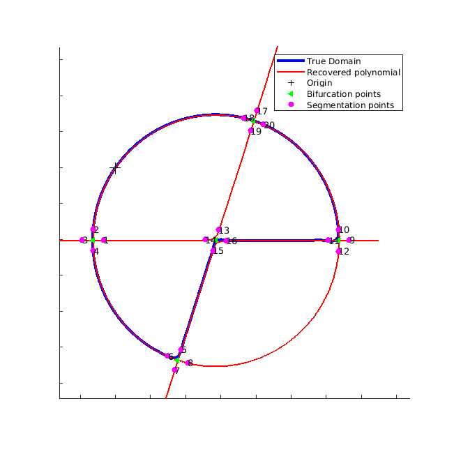
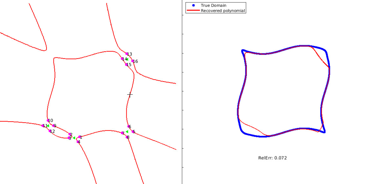
16: end procedureDescription: As seen in Figure 4.3 the bifurcation points seldom lie on the level set. We now seek the nearest points on the level set to a fixed bifurcation point. These segmentation points define the end points of arcs in the level set. Note the double index notation, which is useful for defining arcs. The parameter

N

determines the fineness of the minimization and was fixed at

1000

and left at that.

Refer to caption — Figure 4.2. Recovered polynomial level set with bifurcation and segmentation points.

Algorithm 4.6 Arcs

1: procedure FindArcs(

P(x,y),S,Bound

)

2: TrivArcs

:=\{(ik,il,0):k\neq l\wedge k,l\in M_{i}\penalty\ ,\penalty\ i\in M\}

3: for

[x^{(i)}_{k},y^{(i)}_{k}]\in S

\{[x_{p},y_{p}]:p\in\{1,..,N\}\}=

TraceLvlSet

(P(x,y),s,S\setminus\{s\},1,t_{step})

[x^{(j)}_{l},y^{(j)}_{l}]=:\widehat{s}=argmin_{s^{\prime}\in S\setminus\{s\}}||[x_{N},y_{N}]-s^{\prime}||

6: if

e_{i}\in

TrivArcs or

||[x_{N},y_{N}]||>Bound

then

7: Skip to next segmentation point.

8: else

e_{ik}:=(ik,jl,1)

Positive direction

10:

e_{-ik}:=(jl,ik,2)

Negative direction

11:

E\leftarrow\{e_{ik},e_{-ik}\}

12: end if

13: end for

14:

E\leftarrow

TrivArcs

15: return

E

16: end procedureDescription: The task of this procedure is to find which pairs of segmentation points are connected through the level set. The connection is described as an ordered triple. The first two entries are the indices of the segmentation end points. The third entry is the direction of motion along the level set. Zero is used when the arc does not lie on the level set, see Figure 4.3. The parameter

Bound

here is just to ensure arcs do note race off to infinity.

Algorithm 4.7 Circuits

1: procedure FindCircuits(

E,B,S

)

C^{\prime}\leftarrow

Algorithm from [2]

3: for

c\in C^{\prime}

4: Remove

c

|c|<4

5: Remove

c

|c|>2|B|

6: Remove

c

if it does not containing the origin.

7: Remove

c

if it visits the same bifurcation point twice.

8: Remove

c

if it is a variation of a previous circuit.

9: end for

10: The result is

C\subset C^{\prime}

11: return

C

12: end procedureDescription: This procedure has the goal of making circuits from the previously obtained directed arcs. For clarity this procedure is represented in a more simplified way than the others. The first step is to use a well-known algorithm like the one in [2] in order to find all elementary circuits. Other algorithms are also viable as the arc set is quite small. These circuits represent domain candidates. To reduce the number of candidates, we incorporate some information on the domain. This information takes the form of constraints on the size, inclusion of the origin and internal bifurcation points.

Algorithm 4.8 Constructed Candidate Domains

1: procedure ConstructDomains(

P(x,y),S,C,t_{step},tol

)

2: for

c\in C

3: for

(ik,jl,dir\neq 0):=e\in c

s:=[x^{(i)}_{k},y^{(i)}_{k}]

s^{\prime}:=[x^{(j)}_{l},y^{(j)}_{l}]

\{[x^{(e)}_{j},y^{(e)}_{j}]:j\in[N_{e}]\}

= TraceLvlSet

(P(x,y),s,s^{\prime},dir,t_{step})

7: end for

8: for

(ik,jl,dir=0):=e\in c

\{[x^{(e)}_{j},y^{(e)}_{j}]:j\in[N_{e}]\}\leftarrow

interpolate from other arcs.

10: end for

11:

D^{(c)}:=\bigcup_{e\in c}\{[x^{(e)}_{j},y^{(e)}_{j}]:j\in[N_{e}]\}

12: end for

13:

\mathcal{D}:=\{D^{(c)}\penalty\ :\penalty\ c\in C\}

14: return

\mathcal{D}

15: end procedureDescription: This procedure is used to convert a circuit into a set of boundary points. The circuit can be thought of as a blue print for the domain candidate. This is because the circuit defines the sequence of arcs that constitute a domain. Hence the procedure traces out these arcs using the respective segmentation points as start and stop points. The gaps in between arcs obtained from tracing the level set are filled via interpolation from the existing arcs. The result is a set of domains in the form of a set of boundary points.

Algorithm 4.9 Rank Domains

1: procedure rankDomains(

\mathcal{D},\textbf{TGPT}_{2,1}

)

2: for

D^{(c)}\in\mathcal{D}

3: Export

D^{(c)}

image_{c}.png

4: Read

image_{c}.png

as a curve (see https://github.com/yanncalec/SIES)

5: Compute

\textbf{TGPT}_{2,1}^{(c)}

\overline{c}=argmin_{c}\frac{\|\textbf{TGPT}_{2,c}^{(l)}-\textbf{TGPT}_{2,c}\|}{\|\textbf{TGPT}_{2,c}\|}

\overline{D}\leftarrow D_{\overline{c}}

8: end for

9: return

\overline{D}

10: end procedureDescription: This final procedure is to discern which of the finite set of domain candidates most closely resembles the true domain. The resemblance is determined by the first order TGPT. The reason for the export step is that it sub-samples the domain candidate. Otherwise the recovered domain contains far too many points to be numerically stable.

4.2. Examples

In this section, we apply the algorithm described in the previous subsection to a few examples. We demonstrate its performance by means of a well chosen examples. We also show where the algorithm fails.

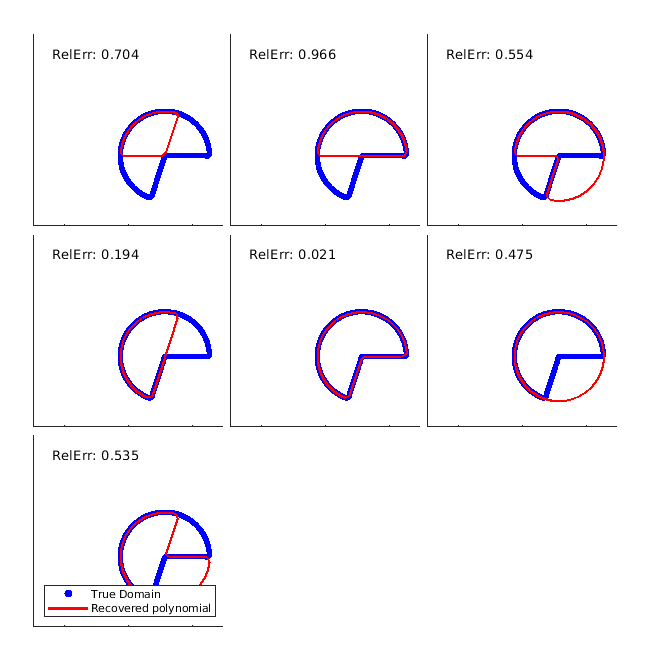
In the first example, Figure 4.7 present the possible seven domain candidates corresponding to a disk with a sector missing shown in Figure 4.6. The true domain is recovered by Algorithm 4.9. Here, it corresponds to the one with relative error $0.021$ .

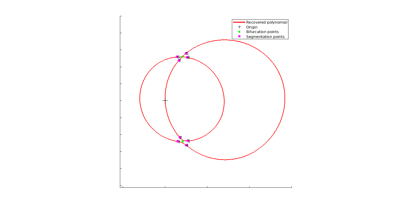
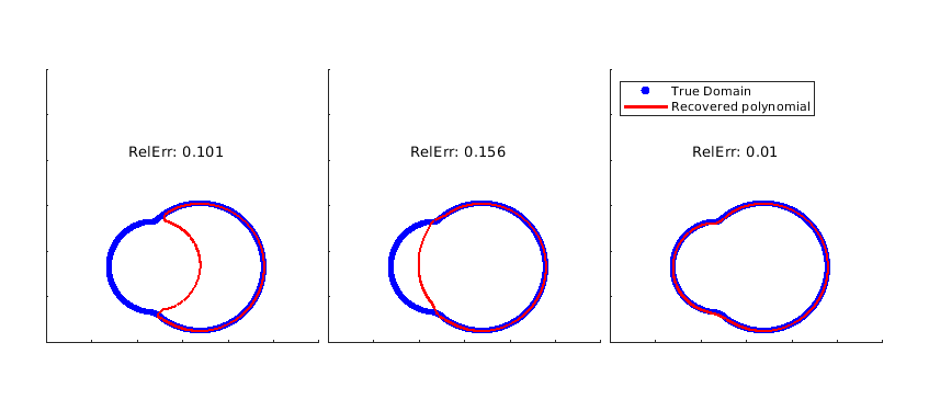
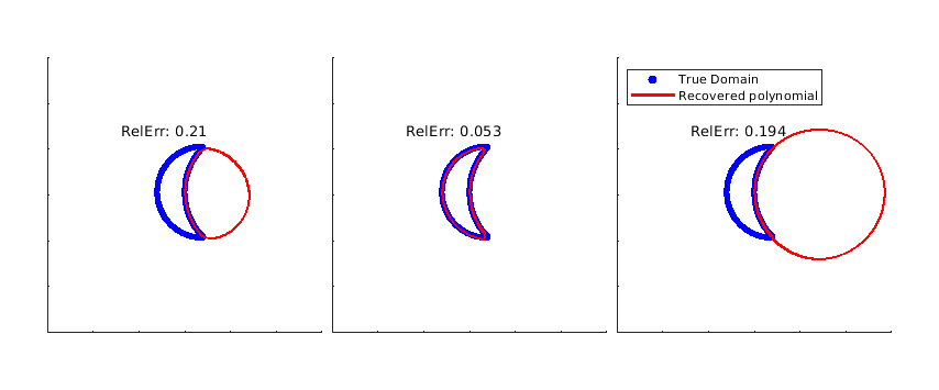
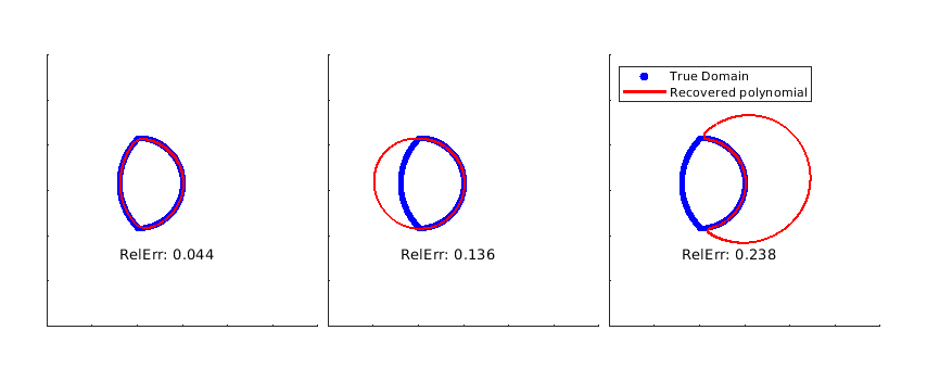
In the second example, we consider domains with the same recovered level set. These are discerned from each other by using some boundary information and matching the associated TGPTs. Figures 4.9, 4.10, and 4.11 show three of the six distinct domains. We call these domains "conjoined circles", "crescent" and "intersection of circles" respectively to indicate the shape. All of these shape have the same level set namely two overlapping circles as seen in Figure 4.8. Among the candidates of the conjoined circles the best candidate was found to have relative error $0.01$ , see Figure 4.9. Among the candidates of the crescent the best candidate was found to have relative error $0.053$ , see Figure 4.10. And among the candidates of the intersection of circles shape the best candidate was found to have relative error $0.044$ , see Figures 4.11.

In the third example, we present in Figure 4.12 a square with sinusoidal sides and its recovery from a single domain candidate.

Finally, we show in Figure 4.13 that sometimes the recovered polynomial simply does not give the right domain. The true domain is in blue while the level set of the reconstructed polynomial from the GPTs is in red. This failure to recover the level set could stem from several reasons. The first reason is that higher degree domains are more unstable due to the higher powers taken in computing their GPTs. The second reason is that the proximity of the origin to a bifurcation point could cause instability. This however is still under investigation. We invite the reader to play around with the algorithm which is open source and available at https://github.com/JAndriesJ/ASPT.

References

[1] Ammari, H., Putinar, M., Steenkamp, A., Triki, F. Identification of an algebraic domain in two dimensions from a finite number of its generalized polarization tensors. Math. Ann. (2018). https://doi.org/10.1007/s00208-018-1780-y
[2] D.B. Johnson, Finding all the elementary circuits of a directed graph, SIAM J. Compt., 4 (1975), 77–84.
[3] H. Ammari, T. Boulier, J. Garnier, W. Jing, H. Kang and H. Wang, Target identification using dictionary matching of generalized polarization tensors, Found. Comput. Math., 14 (2014), no. 1, 27–62.
[4] H. Ammari, J. Garnier, H. Kang, M. Lim, and S. Yu, Generalized polarization tensors for shape description, Numer. Math., 126 (2014), no. 2, 199–224.
[5] H. Ammari, H. Kang, H. Lee, and M. Lim, Enhancement of near cloaking using generalized polarization tensors vanishing structures: Part I: The conductivity problem, Comm. Math. Phys., 317 (2013), no. 1, 253–266.
[6] H. Ammari and H. Kang, Properties of the generalized polarization tensors, SIAM J. Multiscale Modeling and Simulation, 1 (2003), 335–348.
[7] H. Ammari and H. Kang, Polarization and moment tensors with applications to inverse problems and effective medium theory, Applied Mathematical Sciences, Vol. 162, Springer-Verlag, New York, 2007.
[8] H. Ammari and H. Kang, Expansion methods, Handbook of Mathematical Methods of Imaging, 447-499, Springer, 2011.
[9] H. Ammari, H. Kang, M. Lim, and H. Zribi, The generalized polarization tensors for resolved imaging. Part I: Shape reconstruction of a conductivity inclusion, Math. Comp., 81 (2012), 367–386.
[10] H. Ammari, H. Kang, and K. Touibi, Boundary layer techniques for deriving the effective properties of composite materials, Asymptot. Anal. 41 (2005), no. 2, 119–140.
[11] H. Ammari, M. Putinar, M. Ruiz, S. Yu, and H. Zhang, Shape reconstruction of nanoparticles from their associated plasmonic resonances, J. Math. Pures et Appl., 122 (2019), 23–48.
[12] H. Ammari, M. Ruiz, S. Yu, and H. Zhang, Reconstructing fine details of small objects by using plasmonic spectroscopic data, SIAM J. Imaging Sci. 11 (2018), no. 1, 1–23.
[13] H. Ammari, M. Ruiz, S. Yu, and H. Zhang, Reconstructing fine details of small objects by using plasmonic spectroscopic data. Part II: The strong interaction regime, SIAM J. Imaging Sci. 11 (2018), no. 3, 1931–1953.
[14] J. Bochnak, M. Coste, and M.-F. Roy, Real Algebraic Geometry, Springer, Berlin, 1998.
[15] E. Bonnetier, C. Dapogny, and F. Triki, Homogenization of the eigenvalues of the Neumann-Poincaré operator. Preprint (2017).
[16] M. J. de la Puente Real Plane Alegbraic Curves, Expo. Mathematicae, 20 (2002), 291–314.
[17] D. Dubois and G. Efroymson, Algebraic theory of real varieties, in vol. Studies and Essays presented to Yu-Why Chen on his 60-th birthday, Taiwan University, 1970, pp. 107-135.
[18] E. Fabes, M. Sand, and J.K. Seo, The spectral radius of the classical layer potentials on convex domains. Partial differential equations with minimal smoothness and applications (Chicago, IL, 1990), 129–137, IMA Vol. Math. Appl., 42, Springer, New York, 1992.
[19] M. Fatemi, A. Amini, and M. Vetterli, Sampling and reconstruction of shapes with algebraic boundaries, IEEE Trans. Signal Process, 64 (2016), no. 22, 5807–5818.
[20] B. Gustafsson, C. He, P. Milanfar, and M. Putinar, Reconstructing planar domains from their moments, Inverse Problems, 16 (2000), 1053–1070.
[21] B. Gustafsson and M. Putinar, Hyponormal Quantization of Planar Domains, Lect. Notes Math. vol. 2199, Springer, Cham, 2017.
[22] M.-K. Hu, Visual pattern recognition by moment invariants, IRE Trans. Inform. Theory, 8 (1962), 179–187.
[23] J-B Lasserre, and M. Putinar, Algebraic-exponential data recovery from moments, Discrete & Computational Geometry, 54 (2015), 993–1012.
[24] R. Nevanilinna, Analytic functions, Springer (1970) (Translated from German)
[25] G. Taubin, F. Cukierman, S. Sulliven, J. Ponce, and D.J. Kriegman, Parametrized families of polynomials for bounded algebraic curve and surface fitting, IEEE Trans. Pattern Anal. Mach. Intellig., 16 (1994), 287–303.
[26] F. Triki and M. Vauthrin, Mathematical modeling of the Photoacoustic effect generated by the heating of metallic nanoparticles, Quart. Appl. Math. 76 (2018), no. 4, 673–698.