A Logic Framework for P2P Deductive Databases
Abstract
This paper presents a logic framework for modeling the interaction
among deductive databases in a P2P (Peer to Peer) environment.
Each peer joining a P2P system provides or imports
data from its neighbors by using a set of mapping rules,
i.e. a set of semantic correspondences to a set of peers belonging
to the same environment. By using mapping rules, as soon as it
enters the system, a peer can participate and access all data
available in its neighborhood, and through its neighborhood it
becomes accessible to all the other peers in the system.
A query can be posed to any peer in the system and the
answer is computed by using locally stored data and all the
information that can be consistently imported from the neighborhood.
Two different types of mapping rules are defined:
mapping rules allowing to import a maximal set of atoms not leading to inconsistency (called
maximal mapping rules) and mapping rules allowing to import a
minimal set of atoms needed to restore consistency (called minimal mapping rules).
Implicitly, the use of
maximal mapping rules states it is preferable to import as long as no inconsistencies arise; whereas the use of
minimal mapping rules states that it is preferable not to import unless a inconsistency exists.
The paper presents three different declarative semantics of a P2P system:
(i) the Max Weak Model Semantics, in which mapping rules are used to import as much knowledge as possible from a peer’s neighborhood without violating local integrity constraints;
(ii) the Min Weak Model Semantics, in which the P2P system can be locally inconsistent and the information provided by the neighbors is used to restore consistency, that is to only integrate the missing portion of a correct,
but incomplete database;
(iii) the Max-Min Weak Model Semantics that unifies the previous two different perspectives captured by the Max Weak Model Semantics and Min Weak Model Semantics.
This last semantics allows to characterize each peer in the neighborhood as a resource used either to enrich (integrate) or to fix (repair) the knowledge,
so as to define a kind of integrate-repair strategy for
each peer.
For each semantics, the paper also introduces an equivalent and alternative characterization, obtained by rewriting each mapping rule into prioritized rules so as to model a P2P system as a prioritized logic program.
Finally, results about the computational complexity of P2P logic queries, are investigated by considering brave and
cautious reasoning.
Under consideration in Theory and Practice of Logic Programming (TPLP).
KEYWORDS: Peer data Exchange, Incompleteness, Inconsistency, Integrity Constraints, Relational Databa-ses, Prioritized Logic Program.
1 Introduction
Data exchange consists in sharing data from a source schema to a target schema according to specifications fixed by source-to-target constraints [39, 40, 44]. This challenging topic is closely related to data integration and consistent query answering [51, 47, 6, 52, 5, 21, 20]. Data integration is one of the most fundamental processes in intelligent systems, from individuals to societies. At the present, the most important application of data integration is any form of P2P interaction and cooperation. Ideally, in P2P systems there is no selection, but integration of the valuable contributions of every participant.
In a Peer Data Managment System, PDMS, a number of peers interact and exchange data. More specifically, each peer joining a P2P system uses a set of mapping rules, i.e. a set of semantic correspondences to a set of peers belonging to the same environment, to both provide or import data from its neighbors. Therefore, in a P2P system the entry of a new source, peer, is extremely simple as it just requires the definition of the mapping rules. By using mapping rules, as soon as it enters the system, a peer can participate and access all data available in its neighborhood, and through its neighborhood it becomes accessible to all other peers in the system.
The possibility for the users of sharing knowledge from a large number of informative sources, has enabled the development of new methods for data integration easily usable for processing distributed and autonomous data.
Due to this, there have been several proposals which consider the integration of information and the computation of queries in an open ended network of distributed peers [9, 10, 25, 23, 41] as well as the problem of schema mediation [49, 54, 50], query answering and query optimization in P2P environments [1, 61, 48, 39].
Previously proposed approaches investigate the data integration problem in a P2P system by considering each peer as locally consistent. Therefore, the introduction of inconsistency is only caused by the operation of importing data from other peers. These approaches assume that for each peer it is preferable to import as much knowledge as possible.
Our previous works, in the context of P2P data integration, follow this direction.
In [26, 27, 28, 29, 31] it is adopted the classical idea that a peer imports maximal sets of atoms. More specifically, the interaction among deductive databases in a P2P system has been modeled by importing maximal sets of atoms not violating integrity constraints, that is maximal sets of atoms that allow the peer to enrich its knowledge while preventing inconsistency anomalies. The following examples will clarify the perspective used by maximal mapping rules to import in each peer maximal sets of atoms not violating integrity constraints.
Example 1

Consider the P2P system depicted in Figure 1.
- •
Peer stores information about products that should be ordered. It contains the facts:
and . The special syntax used for a fact – its first part is the peer identifier – will be formally presented in Section 3. - •
Peer contains:
- –
the fact , whose meaning is ‘Dan is a supplier of laptops’;
- –
the maximal mapping rule, , whose precise syntax and semantics will be formally defined in Section 3. Intuitively, this rule allows to import as many orders as possible from the relation shopping of into the relation order of . In fact, it states that if is true in the source peer , the atom can be imported in the target peer (that is is true in the target peer) only if it does not imply the violation of some integrity constraints;
- –
the rule stating that a product is available if there is a supplier of
- –
the integrity constraint , stating that the order of a device cannot exist if it is not available.
- –
Intuitively, peer provides two facts, but the maximal set of them that can import, using the mapping rule, is . The fact cannot be imported as it would violate the integrity constraint; in fact, no supplier of the device monitor exists.
Besides the basic classical idea followed in the previous example, a different perspective could be argued. Often, in real world P2P systems, peers use the available import mechanisms to extract knowledge from the rest of the system only if this knowledge is strictly needed to repair an inconsistent local database. The work in [32] stems from this different perspective. A peer can be locally inconsistent and it can use the information provided by its neighbors in order to restore consistency, that is to only integrate the missing portion of a correct, but incomplete database. Then, an inconsistent peer, in the interaction with different peers, just imports the information allowing to restore consistency, that is minimal sets of atoms allowing the peer to enrich its knowledge so as to restore inconsistency anomalies.
The following example will intuitively clarify this perspective.
Example 2

Consider the P2P system depicted in Figure 2. It consists of the following two peers:
- •
Peer stores information about vendors of devices and contains the following facts: , whose meaning is ‘Dan is a vendor of laptops’, and , whose meaning is ‘Bob is a vendor of laptops’.
- •
Peer contains:
- –
the fact , stating that the order of a laptop exists;
- –
the minimal mapping rule , whose precise syntax and semantics will be formally defined in Section 3. The rule is used to import tuples from the relation vendor of into the relation supplier of . Intuitively, the rule states that if is true in the source peer the atom can be imported in the target peer (that is is true in the target peer) only if it implies the satisfaction of some constraints that otherwise would be violated;
- –
the standard rule , stating that a device is available if there is a supplier of ,
- –
the integrity constraint , stating that the order of a device cannot exist if it is not available.
- –
Peer is inconsistent. The integrity constraint is violated as the ordered device laptop is not available (there is no supplier of laptops). The device needs to be provided by a supplier. Therefore, ‘needs’ to import from its neighbors minimal sets of atoms in order to restore consistency. The intuition is that either or can be imported into to satisfy the constraint (but not both).
The two concepts proposed in [26, 27, 28, 29, 31] and in [32] can be merged. The basic idea is that a peer of a P2P system can use each neighbor to extract either as much knowledge as possible (i.e. to integrate its knowledge) or just the portion that is strictly needed (i.e. to repair the knowledge of the system). This unified framework defines a sort of integrate-repair strategy.
The following example will intuitively clarify our perspective and will be used as a running example in the rest of the paper.
Example 3

Consider the P2P system depicted in Figure 3.
- •
Peer stores information about vendors of devices and contains the facts:
, whose meaning is ‘Dan is a vendor of laptops’ and
, whose meaning is ‘Bob is a vendor of laptops’; - •
Peer stores information about devices that should be ordered:
and
; - •
Peer contains:
- –
the integrity constraint
disallowing to import the order of a device that cannot be provided by any supplier. - –
the standard rule
, stating that a device is available if there is a supplier of - –
two mapping rules
- that, intuitively, allows to import as many orders as possible from and
- that allows to import minimal sets of supplier from able to provide the ordered devices.
- –
The intuitive meaning of the P2P system is the following: the fact
, belonging to the adding resource , can be
used to derive . This fact does not violate the
integrity constraint in thanks to the repair resource whose
role is to try to guarantee the consistency of .
In more detail, either
or can be
used to derive the fact and thus to satisfy
the constraint.
Therefore, the preferred scenarios of the system, called max-min weak models, contain besides the base predicates, either the facts
or the
facts .
Observe that, we cannot act in a similar way with respect to the fact
belonging to : no repair mechanism can be
activated in order to support the derived predicate
.
Summarizing, the presence of the repair resource allows the
system to fix the knowledge imported from .
In the previous example, peer aims at
enriching its knowledge by importing from as much
knowledge as possible, and uses to (eventually)
restore inconsistencies. Therefore, with respect to
, peer acts as an adding resource, whereas peer acts as a repair resource.
Different alternative semantics for P2P systems, that will be extensively discussed in Section 6, have been proposed in the literature. In any case, in each of them mapping rules are used as a vehicle to import data.
Our approach, as well as in general P2P data management systems, can be viewed as a special case of Multi-Context Systems (MCS) as it models autonomous logic-based entities (peers) that interchange pieces of information using mapping rules. In any case, the essential feature of P2P system is that each peer may leave and join the system arbitrarily. Due to this specific dynamic nature, the focus in the P2P context is not that of finding the explanations of inconsistencies, but just cope with them. In our work, due to the two different forms of mapping rules, each peer is given the possibility to decide how to interact with a neighbor peer: as a source used to maximize its own knowledge or as a source used to fix its own knowledge. This specific notion has not a counterpart in any of the previous works in the literature, neither in the field of MCS, nor in the field of P2P systems.
Contributions.
The paper presents a logic-based framework for modeling the interaction among peers. It is assumed that each peer consists of a database, a set of standard logic rules, a set of mapping rules of two possible types and a set of integrity constraints. In such a context, a query can be posed to any peer in the system and the answer is provided by using locally stored data and all the information that can be consistently imported from the neighborhood.
In synthesis, the main contributions of the paper are:
- •
The introduction of two different forms of mapping rules: maximal mapping rules used to import maximal sets of atoms while preventing inconsistency anomalies and minimal mapping rules used to fix the knowledge by importing minimal sets of atoms allowing to restore consistency. In other words, maximal mapping rules state that it is preferable to import as long as no local inconsistencies arise; whereas minimal mapping rules state that it is preferable not to import unless a local inconsistency exists. By using, these two forms of mapping rules a generic peer is able to decide how to interact with a neighbor peer: as a source used to maximize its own knowledge or as a source used to fix its own knowledge.
- •
The proposal of the Max Weak Model Semantics, in which mapping rules are used to import as much knowledge as possible from its neighborhood without violating local integrity constraints.
- •
The proposal of the Min Weak Model Semantics, in which the P2P system can be locally inconsistent and the information provided by the neighbors is used to restore consistency, that is to only integrate the missing portion of a correct, but incomplete database.
- •
The Max-Min Weak Model Semantics that unifies the previous two different perspectives captured by the Max and Min Weak Model Semantics. This more general declarative semantics, allows to characterize each peer in the neighborhood as a resource used either to enrich (integrate) or to fix (repair) the knowledge, so as to define a kind of integrate-repair strategy for each peer in the P2P setting.
- •
The definition of an alternative characterization of the Max-Min Weak Model Semantics (resp. Max Weak Model Semantics and Min Weak Model Semantics) obtained by rewriting mapping rules into prioritized rules. Therefore, a P2P system is rewritten into an equivalent prioritized logic program, , such that the max-min weak models of (resp. maximal weak models and minimal weak models) are the preferred stable models of .
- •
Results on the complexity of answering queries. The paper, by considering analogous results on stable model semantics for prioritized logic programs, proves that for disjunction-free () prioritized programs deciding whether an interpretation is a max-min weak model (resp. maximal weak models and minimal weak model) of is complete; deciding whether an atom is true in some max-min weak model (resp. maximal weak models and minimal weak model) is -complete, whereas deciding whether an atom is true in every preferred model is -complete [60]. Moreover, the paper also provides results on the existence of a max-min weak model (resp. maximal weak model and minimal weak model) showing that the problem is in .
- •
An extensive section, Discussion, reporting different features of the proposal. In more detail, the practical aspects of the proposal are highlighted and several additional and alternative issues, arising from the basic framework, are presented: a technique allowing to deal with P2P systems locally inconsistent; a deterministic semantics, derived from the max weak model semantics, allowing to assign a unique three value model to particular types of P2P systems; a polynomial distributed algorithm for its computation; a system prototype.
Structure of the paper.
The remainder of the paper is organized as follows. Section 2 introduces relevant background information. Section 3 describes the syntax of P2P systems. Section 4 describes alternative semantics, namely the Max Weak Model Semantics in [26], the Min Weak Model Semantics in [32] and introduces a new formal declarative semantics, called Max-Min Weak Model Semantics, that unifies the previous two into a more general perspective. Moreover, it introduces, for each of the proposed semantics, an alternative characterization, modeled in terms of logic programs with priorities. Section 5 presents results on computational complexity, Section 6 focuses on some relevant discussions related to practical aspects of the proposed framework and Section 7 introduces a comprehensive discussion of related works. Finally, Section 8 reports concluding remarks and directions for further research.
2 Background
We assume that there are finite sets of predicates, constants and variables [2]. A term is either a constant or a variable. An atom is of the form where is a predicate and are terms. A literal is either an atom or its negation . As in this work we use the Closed World Assumption, we adopt negation as failure. A rule is of the form:
- •
, where is an atom and is a conjunction of literals or
- •
, where is a conjunction of literals.
is called head of the rule and is called body of the rule. A rule of the form is also called constraint. A program is a finite set of rules. is said to be positive if it is negation free.
An exclusive disjunctive rule is the form and it is a notational shorthand for , and 11 1 We use for the operator and both ’,’ and ’’. . Its intuitive meaning is that if is true then exactly one of and must be true.
It is assumed that programs are safe, i.e. variables occurring in the head or in negated body literals are range restricted as they occur in some positive body literal.
An atom (resp. literal, rule, program) is ground if no variable occurs in it. A ground atom is also called fact. The set of ground instances of an atom (resp. literal , rule , program ), denoted by (resp. , , ) is built by replacing variables with constants in all possible ways. An interpretation is a set of facts. The truth value of ground atoms, literals and rules with respect to an interpretation is as follows: , , and , where is an atom, are literals and . An interpretation is a model for a program , if all rules in are true w.r.t. . A model of a program is said to be minimal if there is no model of such that . We denote the set of minimal models of a program with . Given an interpretation and a predicate , denotes the set of -tuples in . The semantics of a positive program is given by its unique minimal model which can be computed by applying the immediate consequence operator until the fixpoint is reached (). The semantics of a program with negation is given by the set of its stable models, denoted as . An interpretation is a stable model of if is the unique minimal model of the positive program , where is obtained from by: (i) removing all rules such that there exists a negative literal in the body of and is in and (ii) removing all negative literals from the remaining rules [46]. It is well known that stable models are minimal models (i.e. ). .
2.1 Prioritized Logic Programs
Several works have investigated various forms of
priorities into logic languages
[15, 17, 36, 60].
In this paper we refer to the extension proposed in [60].
A preference relation among ground atoms is
defined as follows.
For any ground atoms and , if then we say that
has a higher priority than .
stands for and .
The statement is called a priority.
The statement , where and are tuples containing variables, stands
for every priority , where and are instances of and respectively.
If , and do not have common ground instances.
Indeed, assuming that there is a ground atom which
is an instance of and , the statements and
would hold at the same time (a contradiction).
Given a set of priorities, we define the closure as the set of priorities which are reflexively or transitively derived using priorities in .
Let be a class of sets of ground atoms and a set of priorities.
The relation is defined over the sets of
as follows. For any sets and of :
- •
;
- •
if such that and such that ;
- •
if and , then .
If holds, then we say that is preferable to w.r.t. . Moreover, we write if and . A set is a preferred set of if is in and there is no set in such that . The class of preferred sets of will be denoted by . A prioritized logic program (PLP) is of the form where is a logic program and , with , are sets of priorities. The preferred stable models of denoted as are the stable models of selected by applying consecutively the sets of priorities . More formally:
- •
- •
3 P2P Systems
A peer identifier is a number . A (peer) predicate is a pair , where is a peer identifier and is a predicate22 2 Whenever the reference to a peer predicate (resp. peer atom, peer literal, peer fact, peer rule, peer standard rule, peer integrity constraint, peer maximal mapping rule, peer minimal mapping rule) is clear from the context, the term peer can be omitted.. A (peer) atom is of the form , where is a peer identifier, is an atom and is a list of terms. A (peer) literal is a peer atom or its negation . A conjunction , where is a conjunction of built-in atoms33 3 A built-in atom is of the form , where and are terms and . It is also denoted as ., will be also denoted as .
Definition 1
[Peer Rule]. A (Peer) rule can be of one of the following types:
- 1.
(Peer) standard rule.
It is of the form , where and . - 2.
(Peer) integrity constraint.
It is of the form , where , - 3.
(Peer) maximal mapping rule.
It is of the form , where , and . - 4.
(Peer) minimal mapping rule.
It is of the form , where , and .
In the previous definition, (resp. ) is the peer identifier (resp. source peer identifier) of the rule, is the head of the rule and is the body of rule. With the term mapping rule we refer to a maximal mapping rule or to a minimal mapping rule. The concepts of ground rule, fact and interpretation are similar to those reported in Section 2. Given a fact , is its peer identifier.
In our setting, a predicate is of exactly one of the following three types: base predicate, derived predicate
and mapping predicate.
A derived predicate is a predicate occurring in the head of a standard rule, a mapping predicate is a predicate occurring in the head of a mapping rule. If a predicate is neither a derived predicate nor a mapping predicate, then it is a base predicate.
An atom is a base atom (resp. derived atom, mapping atom)
if is a base predicate (resp. derived predicate, mapping predicate).
The intuitive meaning of a standard rule is that whenever its body
is true, its head has to be true.
This meas that an interpretation satisfies a standard rule if
for each ground instance of it, does not satisfy the body of
or satisfies the head of .
The intuitive meaning of an integrity constraint is that its body has to be false.
Therefore, an interpretation satisfies an integrity constraint if
for each ground instance of it, does not satisfy the body of
.
The intuitive meaning of a maximal rule is that whenever its body
is true, its head has to be true if it does not violate (directly or indirectly) any integrity constraint.
Finally, the intuitive meaning of a minimal rule is that whenever its body
is true, its head has to be true if it prevents the violation (directly or indirectly) of some integrity constraint.
In the following sections, we will see how the semantics of a maximal mapping rule and a minimal mapping rule can be captured
by an exclusive disjunctive rule and a priority.
Given an interpretation , (resp. , ) denotes the subset of base atoms (resp. derived atoms, mapping atoms) in .
Definition 2
[P2P SYSTEM]. A peer , with a peer identifier , is a tuple , where
- •
is a set of facts whose peer identifier is equal to (local database);
- •
is a set of standard rules whose peer identifier and source peer identifier are equal to ;
- •
is a set of mapping rules whose peer identifier is equal to and
- •
is a set of constraints over predicates defined by , and whose peer identifier is equal to .
A P2P system is a set of peers s.t. for each source peer identifier occurring in its mapping rules, .
Given a peer , we denote as:
- •
the subset of maximal mapping rules in
- •
the subset of minimal mapping rules in .
Clearly, . Without loss of generality, we assume that every mapping predicate is defined by only one mapping rule of the form (resp. ). Indeed, a mapping predicate consisting of rules of the form , with and , can be rewritten into rules of the form and with . Observe that, becomes a derived predicates and , with , are new mapping predicates. Moreover, there is no loss of generality in considering mapping rules having a positive body. Indeed, allowing negation in the body of mapping rules, a mapping rule , where and , could be rewritten into the mapping rule and the standard rule .
Given a P2P system , where with , the sets , , and denote, respectively, the global sets of ground facts, standard rules, mapping rules, integrity constraints, maximal mapping rules and minimal mapping rules that is:
- •
,
- •
,
- •
,
- •
,
- •
,
- •
In the rest of the paper, with a little abuse of notation, will be denoted both with the
tuple and with the set
.
Moreover, we call a P2P system only containing maximal mapping rules, a maximal P2P system and a P2P system only containing minimal mapping rules, a minimal P2P system.
A peer is locally consistent if . A P2P system whose peers are locally consistent is locally consistent. A peer (resp. P2P system) that is not locally consistent is locally inconsistent.
Given a mapping rule (resp. ), the corresponding standard logic rule will be denoted as .
Analogously, given a set of mapping rules , and given a P2P system , .
In this context an interpretation is a set of peer facts. The truth value of a peer fact (resp. literal, rule, maximal mapping rule, minimal mapping rule) with respect to an interpretation is as follows:
- •
,
- •
,
- •
,
- •
,
- •
,
- •
.
Therefore, while a standard rule is satisfied if its body is false or its body is true and its head is true, a mapping rule is satisfied if its body is true or its body is false and its head is false.
4 Semantics for P2P Systems
Recent literature proposed different semantics for P2P systems that will be discussed in Section 7.
The simplest semantics for a P2P system is the First Order Logic (FOL) semantics obtained by interpreting mapping rules as standard rules. The FOL semantics of a
P2P system is given by the set
of minimal models of .
The problem with the FOL semantics is that it leads to global inconsistency () as soon as an atom imported in a peer
causes a violation of one of its integrity constraints.
It’s clear that more robust semantics, derived by assuming more flexible behaviors of mapping rules, are needed.
It is worth noting that, in the FOL semantics, classical negation is used. In this paper, instead, we adopt negation as failure suited for all the non monotonic semantics here presented.
Our insight is that a peer of a P2P system can use its mapping rules to import from its neighborhood either as much knowledge as possible preserving its consistency or just the knowledge that is strictly needed to restore the consistency of the system.
Starting from this idea, in this section we first present two alternative semantics for P2P systems:
the Max Weak Model Semantics and the Min Weak Model Semantics.
In the Max Weak Model Semantics, the peers of a P2P system only have maximal mapping rules and use them to import maximal sets of facts not violating local integrity constraints.
In the Min Weak Model Semantics, the peers of a P2P system only have minimal mapping rules and use them to import minimal sets of facts that are strictly needed to restore the consistency of the system.
In the Max-Min Weak Model Semantics, the peers of a P2P system have maximal and minimal mapping rules and
unifies the two previous perspectives.
A peer can use each neighbor as a resource either to enrich (integrate) or to fix (repair) its knowledge,
adopting a kind of integrate-repair strategy.
All these semantics guarantee that a P2P system that is
locally consistent admits at least a model, i.e. remains consistent.
In order to present the three different semantics first of all we introduce the concept of weak model, that is common to all of them.
Definition 3
[Weak Model]. Given a P2P system , an interpretation is a weak model for if , where is the program obtained from by:
- •
removing all peer rules such that a negative literal occurs in the body of and is not in ;
- •
removing from the remaining peer rules each negative literal.
- •
removing all mapping rules whose head is not in ;
The set of weak models of will be denoted as .
Observe that, is an Horn program and it
can be partitioned into a set of standard rules , a set of integrity constraints and a set of facts (i.e. ).
As is a positive normal program, it admits exactly one minimal model . Therefore, is the minimal model of if
, otherwise does not admit any minimal model. If then is a weak model of .
Note that,
the definition of weak model presents interesting analogies with the definition of stable model (see Section 2).
Indeed, given a logic program , an interpretation is a stable model of if is the minimal model of the reduct , where the reduct is obtained by removing from each rule such that a negative literal occurs in the body of and is not in and removing from the remaining rules each negative literal.
The fact that is a minimal model of the reduct ensures that each atom is supported, i.e. there is a rule in whose head is and whose body is satisfied by .
Similarly, in Definition 3 the fact
that is a minimal model of ensures that each atom is supported. In particular, for each mapping atom there is a mapping rule in whose head is and whose body is satisfied by .
Example 4

Consider the P2P system depicted in Figure 4. contains the facts and , whereas contains the maximal mapping rule and the constraint . The weak models of the system are , and .
We shall denote with (resp. , , , ) the set of ground atoms of which are defined in (resp. , , , ).
Given a pair , where and are generic objects, (resp. ) denotes the object (resp. ).
The next proposition shows that for a P2P system having only positive rules in , checking if an interpretation is a weak model is simpler because a simpler reduct involving only can be used.
Proposition 1
Given a P2P system s.t. no negation occurs in , an interpretation is a weak model for if and only if , where is the program obtained from by removing all mapping rules whose head is not in .
Proof. can be obtained from by simply removing from
each negative literal s.t. that is
if , then , where is obtained from by removing each negative literal s.t. .
As is a weak model for , it is the minimal model
of and . As all the negative literals
occurring in are s.t. , it follows that . Therefore, is a minimal model of .
If is the minimal model of
, it is the minimal model
of and .
Let us consider an integrity constraint
(observe that, the body of only contains positive literals).
There are the following cases:
- •
. In this case, no negative atom has been removed from the original integrity constraint in order to obtain . We have that and .
- •
. In this case has been obtained from a ground integrity constraint . All negative literals removed from in order to obtain are not in (otherwise could not belong to ). Moreover, . As and each negative literal occurring in is true w.r.t. , at least a positive literal occurring in has to be false w.r.t. . It follows that .
Therefore, and is a minimal model of , that is is a weak model for .
4.1 Max Weak Model Semantics
We recall that a maximal mapping rule (see Definition 1) is of the form . Intuitively, means that if the body conjunction is true in the source peer, the atom will be imported in the target peer (that is is true in the target peer) only if it does not imply (directly or indirectly) the violation of some constraints. In this section, we assume that all mapping rules of a P2P system are maximal mapping rules i.e. is a maximal P2P system.
Example 5
Consider a P2P system consisting of two peers and , where:
In this case, the fact cannot be imported in as it
indirectly violates the integrity constraint.
Definition 4
[Maximal Weak Model]. Given a maximal P2P system and two weak models and of , is said max-preferable to , and is denoted as , if . Moreover, if and , then . A weak model of is maximal if there is no weak model of such that . The set of maximal weak models of will be denoted as .
In the Max Weak Model Semantics peers import maximal sets of facts not violating integrity constraints. Therefore, each peer of the system can be thought as an integration resource. We will show that a locally consistent P2P system always admits a maximal weak model while a locally inconsistent P2P system not always has this property. A generalization of our semantics that guarantees the existence of at least a model even for locally inconsistent P2P system will be presented in a following section.
Example 6
In Example 4 the maximal weak models are and .
The Max Weak Model Semantics easily allows to express a classical problem, the three- colorability problem, as follows.
Example 7
Three-colorability. We are given two peers: , containing a set of nodes and a set of colors which are defined by the unary relations and respectively, and , containing a set of edges defined by the binary relation , the mapping rule:
and the integrity constraints:
stating, respectively, that a node cannot be colored with two different colors and two connected nodes cannot be colored with the same color. The mapping rule states that the node can be colored with the color , only if in doing this no constraint is violated, that is if the node is colored with a unique color and there is no adjacent node colored with the same color. Each maximal weak model computes a maximal subgraph which is three-colorable.
The following proposition shows an important property of relation .
Proposition 2
For any maximal P2P system s.t. no negation occurs in , defines a partial order on the set of weak models of .
Proof. We prove that relation is antisymmetric and transitive.
- •
(Antisymmetry) Let us consider two weak models and in . We prove that if and , then . As , then . Similarly, as , then . It follows that . As and are weak models, by Proposition 1, and . Moreover, as , . It follows that .
- •
(Transitivity) Let us consider three weak models , and in . We prove that if and , then .
As , then . Similarly, as , then . It follows that and then .
If the standard rules of a P2P system contain negation, in general is not antisymmetric. To prove it, let’s consider a P2P system only containing a peer , with the standard rules and . The P2P system admits two weak models: and . As , it follows that and , but .
The next theorem shows that consistent maximal P2P systems always admit maximal weak models.
Theorem 1
For every locally consistent maximal P2P system, .
Proof. Let us consider a set such that , that is a minimal model of a P2P system obtained from by deleting all mapping rules. As is locally consistent, such a model exists. Let be the logic program obtained by deleting from all peer rules whose body is false w.r.t. and by removing from the remaining rules the negative literals (observe that, they are true w.r.t. ). is an Horn program and admits only one minimal model. This minimal model has to be . Moreover, as does not contain any mapping atoms, . It follows that . This means that is a weak model for . As there is at least a weak model of , then .
If a P2P system contains at least a locally inconsistent peer, the Max Weak Model semantics does not guarantee the existence of a maximal weak model.
Example 8
Let us consider a P2P system containing only peer . Clearly, is locally inconsistent and there is no way to import mapping atoms able to restore its consistency. Observe that, the only way to make the peer consistent is to remove at least one fact from its local database. In the following, we present an extension of our framework allowing deletions of facts from local databases.
4.1.1 An Alternative Characterization of the Max Weak Models Semantics
In this section, we present an alternative characterization of the Max Weak Model Semantics based on the rewriting of
mapping rules into prioritized rules [17, 60].
Definition 5
[Rewriting of a Maximal P2P System into a Prioritized Logic Program]. Given a maximal P2P system and a maximal mapping rule , then:
- •
denotes the pair , consisting of a disjunctive mapping rule and a priority statement,
- •
and
- •
.
In the above definition the atom (resp. ) means that the fact is imported (resp. not imported) in the peer .
Intuitively, the rewriting of the maximal mapping rule states that if is true in the source peer then two alternative actions can be performed in the target peer: can be either imported or not imported; but the presence of the priority statement establishes that the action of importing is preferable over the action of not importing .
Example 9
The rewriting of the P2P system in Example 4 is:
has three stable models:
,
,
.
The set of preferred stable models are .
Example 10
Given a maximal P2P system and a preferred stable model for ,
we denote with the subset of non-primed atoms of and
we say that is a preferred stable model of .
We denote the set of preferred stable models of as .
The following theorem shows the equivalence of
preferred stable models and maximal weak models.
Theorem 2
[Equivalence Between Preferred Stable Models and Maximal Weak Models]. For every maximal P2P system , .
Proof.
- 1.
()
Let and . First we prove that is a weak model. Let us consider a ground mapping rule and its rewriting . The rule is equivalent to the rules , and the constraint . There are three cases:- •
. In this case, . Then the bodies of and are false and so .
- •
and . In this case the body of is false and . Moreover, .
- •
and . In this case the body of is false and . Moreover, .
Then, by construction, we have that .
We have that:
- •
The minimal model of is , as is a stable model of ;
- •
;
- •
Non primed atoms can be only inferred by rules in and
- •
No primed atom occurs in the body of any rule of .
Therefore, the minimal model of is and is a weak model of .
Now we prove that is a maximal weak model of . Let us assume by contradiction that there is a weak model such that . Then the ground mapping rules that will be deleted from to derive are a subset of those that will be deleted to to derive .Let us consider the set . By construction, is the minimal model of . Then is a stable model of . Observe that, must exist two atoms and and, by construction, there cannot exist two atoms and . Moreover, contains the preference . Therefore, and is not a preferred stable model of . This is a contradiction.
- •
- 2.
()
Let and . First we prove that is a stable model of i.e. it is the minimal model of .By construction,
.
We have that:
- •
The minimal model of is , as is a weak model of ;
- •
The minimal model of is ;
- •
Non primed atoms can be only inferred by rules in and
- •
No primed atom occurs in the body of any rule of .
Therefore, the minimal model of is and is a stable model of .
Now we prove that is a preferred stable model for . Let us assume by contradiction that there is a stable model for s.t. . From point 1. and preferences in , we have that is a weak model for and , that is is not a maximal weak model for . This is a contradiction.
- •
This characterization of the Max Weak Model Semantics makes evident that importing a mapping atom is preferable over not importing it and provides a computational mechanism allowing to derive the maximal weak models of a maximal P2P system.
Example 11
Consider the P2P system of Example 9, we have:
.
This example shows that the preferred stable models of coincide with its maximal weak models.
4.2 Min Weak Model Semantics
In [32] the authors introduced the Min Weak Model Semantics: a peer can be locally inconsistent and the P2P system it joins provides support to restore its consistency.
The basic idea, yet very simple, is the following:
an inconsistent peer, in the interaction with
other peers, just imports the missing part of its local database which is correct, but incomplete.
The proposal of the Min Weak Model Semantics stems from the observations
that in real world P2P systems, peers often use the available import mechanisms
to extract knowledge from the rest of the system only if this knowledge
is strictly needed to repair inconsistencies of the system.
A minimal mapping rule (see Definition 1) is of the form . Intuitively, means that if the body conjunction is true in the source peer the atom is imported in the target peer (that is is true in the target peer) only if it implies (directly or indirectly) the satisfaction of some constraints that otherwise would be violated. In this section, we assume that all mapping rules of a P2P system are minimal mapping rules i.e. is a minimal P2P system.
Definition 6
[Minimal Weak Model]. Given a minimal P2P system and two weak models and of , is said min-preferable to , and is denoted as , if . Moreover, if and then . A weak model of is said to be minimal if there is no weak model of such that . The set of minimal weak models will be denoted by .
Next example will clarify the concept of minimal weak model.
Example 12
Consider the P2P system presented in Example 2.
The weak models of the system are:
,
and
,
whereas the minimal weak models are
and because they contain minimal subsets of mapping atoms
(resp. and ).
We observe that, adopting the Min Weak Model Semantics, if each peer of a P2P system is locally consistent then no mapping atom is inferred. Clearly, not always a minimal weak model exists. This happens when there is at least a peer which is locally inconsistent and there is no way to import mapping atoms that could repair its local database so that its consistency can be restored.
Example 13
Let us consider the simple P2P system presented in Example 8. Also adopting the Min Weak Model Semantics, does not admit any minimal weak model.
It is important to observe that a peer uses its minimal mapping rules to import minimal sets of atoms allowing the satisfaction of integrity constraints belonging not only to it but also to other peers.
Example 14

Consider the P2P system depicted in Figure 5.
- •
Peer contains the fact
- •
Peer contains the minimal mapping rule
- •
Peer contains the fact , the minimal mapping rule and the integrity constraint .
Peer imports the atom from to guarantee the satisfaction of an integrity constraint belonging to . Min Weak Model Semantics assigns to the system its unique minimal weak model: .
The following proposition shows an important property of relation .
Proposition 3
For any maximal P2P system s.t. no negation occurs in , defines a partial order on the set of weak models of .
Proof. We prove that relation is antisymmetric and transitive.
- •
(Antisymmetry) Let us consider the weak models and in . We prove that if and , then . As , then . Similarly, as , then . It follows that . As and are weak models, by Proposition 1, and . Moreover, as , . It follows that .
- •
(Transitivity) Let us consider the weak models , and in . We prove that if and , then .
As , then . Similarly, as , then . It follows that and then .
In the Min Weak Model Semantics a peer may import an atom from a neighbor peer even if such atom is not needed to repair its own inconsistency, but is needed to restore the consistency of a different peer. In this way, the system behaves in a global way.
4.2.1 An Alternative Characterization of the Min Weak Models Semantics
Similarly to Section 4.1.1, here we present an alternative characterization of the Min Weak Model Semantics
based on the rewriting of
mapping rules into prioritized rules [17, 60].
Definition 7
[Rewriting of a Maximal P2P System into a Prioritized Logic Program]. Given a minimal P2P system and a mapping rule , then:
- •
denotes the pair , consisting of a disjunctive mapping rule and a priority statement,
- •
and
- •
.
In the above definition, the atom (resp. ) means that the fact is imported (resp. not imported) in the peer .
Intuitively, the rewriting of the mapping rule states that if is true in the source peer then two alternative actions can be performed in the target peer: can be either imported or not imported; but the presence of the priority statement establishes that the action of not importing is preferable over the action of importing .
Example 15
Consider again the system presented in Example 2.
The rewriting of the system is:
has three stable models:
,
,
.
The preferred stable models are and .
The following theorem shows the equivalence of preferred stable models and minimal weak models.
Theorem 3
[Equivalence Between Preferred Stable Models and Minimal Weak Models]. For every minimal P2P system , .
Proof.
- 1.
()
Let and . First we prove that is a weak model. Let us consider a ground mapping rule and its rewriting . The rule is equivalent to the rules , and the constraint . There are three cases:
- •
. In this case, . Then the bodies of and are false and so .
- •
and . In this case the body of is false and . Moreover, .
- •
and . In this case the body of is false and . Moreover, .
Then, by construction, we have that .
We have that:
- •
The minimal model of is , as is a stable model of ;
- •
;
- •
Non primed atoms can be only inferred by rules in and
- •
No primed atom occurs in the body of any rule of .
Therefore, the minimal model of is and is a weak model of .
Now we prove that is a minimal weak model of . Let us assume by contradiction that there is a weak model such that . Then the ground mapping rules that will be deleted from to derive are a superset of those that will be deleted to to derive .Let us consider the set . By construction, is the minimal model of . Then is a stable model of . Observe that must exist two atoms and and, by construction, there cannot exist two atoms and . Moreover, contains the preference . Therefore, and is not a preferred stable model of . This is a contradiction.
- •
- 2.
()
Let and . First we prove that is a stable model of i.e. it is the minimal model of .
By construction, . We have that:
- •
The minimal model of is , as is a weak model of ;
- •
The minimal model of is ;
- •
Non primed atoms can be only inferred by rules in and
- •
No primed atom occurs in the body of any rule of .
Therefore, the minimal model of is and is a stable model of .
Now we prove that is a preferred stable model for . Let us assume by contradiction that there is a stable model for s.t. . From point 1. and preferences in , we have that is a weak model for and , that is is not a minimal weak model for . This is a contradiction.
- •
This characterization of the Min Weak Model Semantics makes evident that not importing a mapping atom is preferable over importing it and provides a computational mechanism allowing to derive the minimal weak models of a minimal P2P system.
4.3 Max-Min Weak Model Semantics
This section presents a unified semantics for P2P systems, the Max-Min Weak Model Semantics, that represents a generalization of those introduced in
Section 4.1 and Section 4.2.
A peer, which can be locally inconsistent, can use two import mechanisms for importing knowledge from other peers: maximal mapping rules to import maximal sets of mapping atoms not violating local integrity constraints and minimal mapping rules
to restore local consistency.
These two mechanisms can be combined and used in the same peer. With this semantics, a peer
can consider each of its neighbors as a resource
used either to enrich (integrate) or to fix (repair) its knowledge,
so as to define a kind of integrate-repair strategy.
Example 16
Consider again the P2P system presented in Example 3. As we observed, peer is locally consistent. It imports from all the orders that can be satisfied by suppliers imported from peer . Moreover, a minimum set of suppliers will be imported in .
The fact will be imported in from because there is at least a supplier of the object ‘laptop’ that can be imported in from . Instead, there is no way to import a supplier of the object ‘monitor’. Therefore, the fact will not be imported in . Finally, there are two possible ways to import a supplier of the object ‘laptop’: importing from either the fact or the fact .
Definition 8
[Max-Min Weak Model.] Given a P2P system and two weak models and of , we say that is max-min-preferable to , and we write , if
- •
or
- •
and
Moreover, if and we write . A weak model is said to be max-min if there is no weak model such that . The set of max-min weak models will be denoted by .
The above definition states that a weak model is a max-min weak model if it maximizes the set of atoms imported by means of maximal mapping rules while minimizing the set of atoms imported my means of minimal mapping rules (used to maintain local consistency). The approach follows the classical and natural strategy of enriching as much as possible the knowledge of an information source (by means of maximal mapping rules) guaranteeing consistency (by using minimal mapping rules).
Example 17
Consider the P2P system presented in Example 3.
The weak models of the system are:
,
,
,
,
,
,
.
whereas the max-min weak models are and .
The following proposition shows an important property of relation . It is easy to show that a locally consistent P2P system always admits a max-min weak model.
Proposition 4
For any maximal P2P system s.t. no negation occurs in , defines a partial order on the set of weak models of .
Proof. We prove that relation is antisymmetric and transitive.
- •
(Antisymmetry) Let us consider the weak models and in . We prove that if and , then . As , then or and . Similarly, as , then or and . As the conditions and cannot holds at the same time, it follows that and , that is . As and are weak models, by Proposition 1, and . Moreover, as , . It follows that .
- •
(Transitivity) Let us consider the weak models , and in . We prove that if and , then .
If and , then and so .
If , and , then and so .
If , , and , then and so .
If , , and , then , and so .
4.3.1 An Alternative Characterization of the Max-Min Weak Models
Similarly to Section 4.1.1 and Section 4.2.1, this section presents an alternative characterization of the Max-Min
Weak Model Semantics based on the rewriting of mapping rules into
prioritized rules [17, 60].
Given an atom
we denote as the atom
.
Definition 9
[Rewriting of a P2P System into a Prioritized Logic Program]. Given a P2P system and the mapping rules and , then:
- •
denotes the pair
, - •
denotes the pair
, - •
denotes the pair
- •
denotes the pair
and - •
denotes the prioritized logic program
.
In the above definition, the atom (resp. ) means that the
fact is imported in peer (resp. is imported in peer ).
Intuitively, the rewriting of the maximal (resp. minimal) mapping rule states that
if (resp. ) is true in the source peer then
two alternative actions can be performed in the target peer: (resp. ) can be either imported or not imported; but the presence of the priority statement (resp. ) establishes that the action of importing is preferable over the
action of not importing (resp. the action of not importing is preferable over the
action of importing ).
Observe that, is a prioritized logic program with two levels of priorities. The one applied as first models the preference to import as much maximal mapping atoms as possible. The other one, applied over the models selected in the first step, expresses the preference to import as less minimal mapping atoms as possible.
Example 18
Consider again the system reported in Example 3.
The rewriting of the system is:
},
The logic program has the following stable models:
,
,
,
,
,
,
,
The preferred stable models are and .
Given a P2P system and a preferred stable model for we denote with the subset of non-primed atoms of and we say that is a preferred stable model of . We denote the set of preferred stable models of as .
The following theorem shows the equivalence of preferred stable models and max-min weak models.
Theorem 4
[Equivalence Between Preferred Stable Models and Max-Min Weak Models]. For every P2P system , .
Proof.
- 1.
()
Let and . First we prove that is a weak model. Let us consider a ground mapping rule and its rewriting . The rule is equivalent to the rules , and the constraint . There are three cases:
- •
. In this case, . Then the bodies of and are false and so .
- •
and . In this case the body of is false and . Moreover, .
- •
and . In this case the body of is false and . Moreover, .
Then, by construction, we have that .
We have that:
- •
The minimal model of is , as is a stable model of ;
- •
;
- •
Non primed atoms can be only inferred by rules in and
- •
No primed atom occurs in the body of any rule of .
Therefore, the minimal model of is and is a weak model of .
Now we prove that is a preferred weak model of . Let us assume by contradiction that there is a weak model such that or . Let us consider these cases:- •
(). In this case, the ground maximal mapping rules that will be deleted from to derive are a subset of those that will be deleted to to derive .
Let us consider the set . By construction, it is the minimal model of . Then is a stable model of . Observe that must exist two atoms and and, by construction, there cannot exist two atoms and . Moreover, contains the preference . Therefore, and is not a preferred stable model of . This is a contradiction.
- •
(). In this case, the maximal mapping rules that will be deleted from to derive coincide with those that will be deleted to derive . Moreover, the ground minimal mapping rules that will be deleted from to derive are a superset of those that will be deleted to to derive .
Let us consider the set . By construction, it is the minimal model of . Then is a stable model of . Observe that, must exist two atoms and and, by construction, there cannot exist two atoms and . Moreover, contains the preference . Therefore, and is not a preferred stable model of . This is a contradiction.
- •
- 2.
()
Let and . First we prove that is a stable model of i.e. it is the minimal model of .
By construction, 1 . We have that:
- •
The minimal model of is , as is a weak model of ;
- •
The minimal model of is ;
- •
Non primed atoms can be only inferred by rules in and
- •
No primed atom occurs in the body of any rule of .
Therefore, the minimal model of is and is a stable model of .
Now we prove that is a preferred stable model for . Let us assume by contradiction that there is a stable model for s.t. . From point 1. and preferences in , we have that is a weak model for and or , that is is not a max-min weak model for . This is a contradiction.
- •
This characterization of the Max-Min Weak Model Semantics provides a computational mechanism allowing to derive the max-min weak models of a P2P system.
5 Query Answers and Complexity
We consider now the computational complexity of calculating max-min weak models and answers to queries [57]. As a P2P system may admit more than one max-min weak model, the answer to a query is given by considering brave or cautious reasoning (also known as possible and certain semantics). Issues related to the distributed computation will be discussed in Section 6.3.
Definition 10
Given a P2P system and a ground peer atom , then is true under
- •
brave reasoning if ,
- •
cautious reasoning if .
We assume here a simplified framework not considering the distributed complexity as we suppose that the complexity of communications depends on the number of computed atoms which are the only elements exported by peers.
Theorem 5
Let be a P2P system, then:
- 1.
Deciding whether an interpretation is a max-min weak model of is complete.
- 2.
Deciding whether a max-min weak model for exists is in .
- 3.
Deciding whether an atom is true in some max-min weak model of is complete.
- 4.
Deciding whether an atom is true in every max-min weak model of is complete.
Proof
- 1.
(Membership) We prove that the complementary problem, that is the problem of checking whether is not a max-min weak model, is in . We can guess an interpretation and verify in polynomial time that (i) is a weak model, that is , and (ii) either is not a weak model, that is , or , that is or . Therefore, the original problem is in .
(Hardness) We will reduce the SAT problem to the problem of checking whether a weak model is not max-min. Let be a set of variables and a CNF formula over . Then the problem that will be reduced is checking whether the QBF formula is . We define a P2P system with two peers: and . Peer contains the atoms:The relation stores the variables in and the relation stores the truth values and .
Peer contains the atoms:the mapping rule:
stating that the truth value could be assigned to the variable ,
the standard rules:defining a from the occurrences of its positive and negated variables (first and second rule), whether a clause holds with a given assignment of values (third and fourth rule) and whether an assignment of values actually exists (fifth rule), and the integrity constraints:
stating that two different truth values cannot be assigned to the same variable (first constraint), that if there is an assignment then there cannot be an unsatisfied clause (second constraint) and cannot be an unevaluated variable (third constraint). Let the set of atoms in , the set of mapping rules in , the set of standard rules in and the set of integrity constraints in . Let be the minimal model of , that is the model containing no mapping atom. As is locally consistent, is a weak model of . Observe that, the integrity constraints in are satisfied when no mapping atom is imported in that is if no assignment of values is performed for the variables in . If is not satisfiable, then there is no way to import mapping atoms in preserving consistency because the second constraint will be violated. In this case is a max-min weak model. If is satisfiable there is a weak model whose set of mapping atoms corresponds to an assignment of values to the variables in that satisfies . Clearly, as , is not a max-min weak model. Moreover, if is not a max-min weak model there must be another weak model whose set of mapping atoms corresponds to an assignment of values to the variables in that satisfies . In other words, is satisfiable if and only if is not a max-min weak model.
- 2.
Let us guess an interpretation . By (1), deciding whether is a max-min weak model can be decided by a call to a oracle.
- 3.
From Theorem 4, an atom is in some max-min weak model of if and only if it is true in some preferred stable model of . The complexity of this problem has been presented in [60]. For disjunction-free () prioritized logic programs, deciding whether an atom is true in some preferred stable model is complete.
- 4.
From Theorem 4, an atom is in every max-min weak model of if and only if it is true in every preferred stable model of . The complexity of this problem has been presented in [60]. For disjunction-free () prioritized logic programs, deciding whether an atom is true in every preferred stable model is complete.
6 Discussion
This section introduces some useful discussions on some features of the proposed semantics.
6.1 Dealing with Locally Inconsistent P2P Systems
The framework presented so far does not guarantee that a locally inconsistent P2P system (i.e. containing at least a locally inconsistent peer) has a weak model.
Indeed, there could be locally inconsistent peers that cannot reach a consistent state by importing sets of atoms from other peers.
This happens because the only mechanism modeled by
our original framework is an ‘enriching’ mechanism that does not allow deletions of atoms from local databases.
Therefore, if a peer is locally inconsistent and there is no way to
import mapping atoms able to restore its consistency, the peer remains inconsistent because no atom can be deleted.
In this section, we present an extension of our framework that
simulates deletions of atoms by using maximal mapping rules.
Informally, the idea is to create for each peer an auxiliary peer, move the database from the original peer to the auxiliary one and equip the original peer with a set of
maximal mapping rules allowing to import, from the auxiliary peer, maximal sets of atoms
not violating its integrity constraints.
Definition 11
Let and , with , a peer in .
Then, is the set containing the following peers:
- •
- •
, where
Moreover:
In the previous definition, peer is derived from peer by deleting its local database and inserting a set of maximal mapping rules allowing to import facts into the old base relations (which now are mapping relations) from the auxiliary peer .
Given a P2P system , we define .
We now present a generalization of our semantics allowing to deal with locally inconsistent P2P systems.
Definition 12
Let . The generalized weak models of , denoted as , are obtained from the weak models of by removing all the atoms with .
Definition 13
[Generalized Max-Min Weak Model] Given a P2P system and two generalized weak models and of , we say that is G-preferable to , and we write , if
- •
or
- •
and or
- •
and and
Moreover, if and we write . A weak model is said to be a generalized Max-Min weak model if there is no weak model such that . The set of generalized Max-Min weak models will be denoted by .
Example 19
Consider the P2P system depicted in Figure
6. contains the facts and , whereas
contains
the minimal mapping rule ;
the constraint stating that the base relation can contain at most one tuple, the constraint stating that if contains the fact then the fact has to be derived; and the facts and .
This P2P system is inconsistent because the local database of peer
violates the constraint .
is depicted in Figure 7.

The generalized Max-Min weak models of are:
- •
- •
.
Observe that if contains negation this technique does not guarantee that consistency can be achieved.
6.2 Computing the Max Weak Model Semantics
This section recalls an alternative characterization of the
max weak model semantics that allows to model a maximal P2P system , where only contains positive peer standard rules, with a single disjunctive logic program embedding the set of priorities presented in Section 4.3.1 [28].
In [28] it has been shown that the stable models of correspond to the maximal weak models of .
Using this rewriting, the computation of the preferred
weak models of a P2P system can be performed in a centralized way by using an inference engine like DLV [52] able to process
and compute its stable models.
Although this approach is still not pragmatic, because the computation
is centralized and its complexity is prohibitive for real cases,
the program can be used as a starting
point for a distributed technique, as will be pointed out in
Section 6.3.
The formal details of this approach are out of the scope of this
section and can be found in [28].
Here we want to show how to make our
approach pragmatic by implementing a derived version of max weak model
semantics into a real P2P system.
Let’s firstly introduce some concepts and definitions.
Given a peer atom , denotes the atom and denotes the atom .
is called testing atom, whereas is called violating atom.
A testing atom corresponds to the mapping atom that could be derived in the target peer.
While is derived only if its existence does not cause any inconsistency,
is always derived in order to test whether can be inferred safely.
If the presence of violates at least one
integrity constraint, the corresponding violating atom is derived.
In this case, the atom blocks the derivation of and the inconsistency that would cause is prevented.
Definition 14
Given a conjunction
| (1) |
where () is a mapping atom or a derived atom, () is a base atom and is a conjunction of built in atoms, we define
| (2) |
From the previous definition it follows that given a negation free conjunction of the form
| (3) |
then
| (4) |
Definition 15
[Rewriting of an integrity constraint]. Given an integrity constraint44 4 Recall that is of the form (1). , its rewriting is defined as .
If the body (that is of the form (2)), in the previous definition is true, then it can be deduced that at least one of the violating atoms is true. This states that in order to avoid inconsistencies, at least one of the atoms cannot be inferred.
Definition 16
[Rewriting of a standard rule]. Given a standard rule44footnotemark: 4 , its rewriting is defined as .
In order to find the mapping atoms that, if imported, generate some inconsistencies
(i.e. in order to find their corresponding violating atoms), all possible
mapping testing atoms are imported and the derived testing atoms are inferred.
In the previous definition, if (that is of the form (4)),
is true and the violating atom is true, then the body of the disjunctive rule
is true and therefore it can be deduced
that
at least one of the
violating atoms is true (i.e. to avoid such inconsistencies
at least one of atoms cannot be inferred).
Definition 17
[Rewriting of a maximal mapping rule] Given a mapping rule55 5 Recall that is of the form (3). , its rewriting is defined as .
Intuitively, to check whether a mapping atom generates some inconsistencies, if imported in its target peer, a testing atom is imported in the same peer. Rather than violating some integrity constraint, it (eventually) generates, by rules obtained from the rewriting of standard rules and integrity constraints, the atom . In this case , cannot be inferred and inconsistencies are prevented.
Definition 18
[Rewriting of a Maximal P2P system] Given a Maximal P2P system , then
- •
- •
- •
- •
Example 20
The stable models of are:
Definition 19
[Total Stable Model] Given a P2P system and a stable model for , the interpretation obtained by deleting from its violating and testing atoms, denoted as , is a total stable model of . The set of total stable models of is denoted as .
Example 21
For the P2P system reported in Example 20, .
In [28] it has been shown that the set of total stable models is equivalent to the set of maximal weak models, i.e. .
Observe that, this rewriting technique allows computing
the maximal weak models of a P2P system with an arbitrary topology.
The topology of the system will be encoded in its rewriting.
As an example, if a system is cyclic, its rewriting
could be recursive.
6.3 A System Prototype
The rewriting presented in the previous section has been used in
[28, 34, 33]
as a starting point to implement a system prototype of a P2P
system based on a deterministic version of our maximal weak model
semantics.
The first important observation is that a P2P system may admit many maximal weak models whose computational complexity has been shown to be prohibitive.
Therefore, it is needed to look for
a more pragmatic solution for assigning a semantics to a P2P system. Starting from this observation, a deterministic
model whose computation is guaranteed to be polynomial time has been proposed in [28, 34, 33].
The new proposed semantics, called well founded semantics, assigns to a P2P system its Well Founded Model, a three valued partial deterministic model that captures the intuition that if an atom is true in a maximal weak model and it is false in another one,
then it is undefined in the well founded model [45, 53].
It has been shown that, given a maximal P2P system whose standard rules are positive, the rewriting presented in Section 6.2 is Head Cycle Free [8].
Therefore, it can be normalized obtaining a normal program that we denote as .
The next step is to adopt for a Well Founded Model
Semantics. The program,
admits a well founded model that can be computed in polynomial time.
Example 22
Consider the P2P system presented in Example 4.
The normal version of the rewriting presented in Example 20 is:
;
The well founded semantics of is given by the well founded model of , 66
6
The first component of the pair is the set of true facts while the second one is the set of false facts..
The facts and are true, while the facts
and are undefined.
Although the adoption of a well founded model for a maximal P2P system represents a step forward in the implementation of a real system prototype – as it can be computed in polynomial time–
it is evident that the evaluation of a unique logic program requires a centralized computation and this is not
realistic: a distributed computation is needed.
In [34, 33] a technique allowing to compute the well founded model in a distributed way has been presented.
The basic idea is that each peer computes its own portion of , sending the result to the other peers.
In more detail, if a peer receives a query, then it recursively queries the peers to which
it is connected through mapping rules, before being able to calculate its answer.
Formally, a local query submitted by a user to a peer does not differ from a remote query submitted by another peer.
The only substantial difference is in the construction of the answer that in the case of remote query, must be returned to the requesting peer.
Once retrieved the necessary data from neighbor peers, the peer computes its well founded model and evaluates the query (either local or remote) on that model. If the query is a remote query, the answer is sent to the requesting peer.
Details on the architecture and implementation of
this system prototype can be found in [33].
The paper in [33] also reports an application scenario related to the integration of biomedical data from PubMed (http://www.ncbi.nlm.
nih.gov/pubmed/).
The experiment has been conducted by considering three peers: Peer1, Peer2 and Peer3. Peer1 contains information about papers related to the HIV virus, Peer2 about papers related to the Ebola virus and Peer3 integrates data provided by Peer1 and Peer2. The final aim of this experiment is the integration of all the papers related to both HIV and Ebola virus into a unique data source in Peer3.
7 Related Works
Semantic Peer Data Management Systems.
The present paper is placed among the works on semantic peer data management systems. This research topic formally started with the work in [49] in which the problem of schema mediation in a P2P system is investigated A formalism, , for mediating peer schemas, which uses the GAV and LAV [51] formalism to specify mappings, is proposed. Mappings relate two conjunctive queries expressed in terms of the schema of disjoint peers. The semantics is assigned using classical first-order logic (FOL) and query answering is defined by extending the notion of certain answer. More specifically, certain answers for a peer are those that are true in every global instance that is consistent with local data. This choice implies, as a consequence, the need for the consistency of each peer with respect to the whole P2P system. As for a comparison, in this paper we do not adopt a FOL interpretation for a P2P system and tolerate inconsistencies. A mapping rule [49] is a logical implication between two peers. It is often the case that preference is given to external data over internal data, or equivalently by using the concept of trust given in [12] denotes that the peer trusts itself less than . This paper formalizes a different proposal: mapping rules are a means used either to import maximal sets of atoms while preventing inconsistency anomalies or to fix the knowledge by importing the minimal sets of atoms allowing to restore consistency. In both cases, in our basic framework, we implicitly satisfy the preference that a peer trusts more its own data over data provided by other peers.
In [25] a sound, complete and terminating procedure that returns the certain answers to a query submitted to a peer, is proposed. The paper presents a semantics for a P2P system, based on epistemic logic. Mapping rules between two peers and are of the form , where and are conjunctive queries over the schema of and . An advantage of this framework is that certain answers of fixed conjunctive queries posed on a peer can be computed in polynomial time. The proposal does not manage local inconsistency. Each peer has to be consistent with respect to its integrity constraints, otherwise the entire P2P system is considered inconsistent. Moreover, if inconsistencies arise due to mapping rules the whole P2P system is considered inconsistent. An extension of the epistemic theory that ensures local inconsistency tolerance has been presented in [24]. The paper extends the epistemic theory with an additional operator so as to tolerate local inconsistency. More specifically, it ignores a peer inconsistent with respect to its own local constraints. No consistency restoration process is proposed; on the contrary in our proposal an inconsistent peer is not cut off of the system, but can be repaired by means of mapping rules so as to restore consistency.
In [41, 43, 42] a characterization of P2P database
systems and a model-theoretic semantics dealing with inconsistent
peers is proposed. The basic idea is that if a peer does not have
models all the (ground) queries submitted to the peer are true
(i.e. are true with respect to all models). Thus, if some
databases are inconsistent it does not mean that the entire system
is inconsistent.
The semantics in [41] coincides with
the epistemic semantics in [25, 19].
The semantics in [41, 43, 42]
also provides a distributed algorithm to compute queries; the setting assumes the existence of a super peer instructor that updates peers’ data. The proposal is not inconsistency tolerant as the arise of an inconsistency causes the entire P2P system to became inconsistent.
As for a comparison with the present proposal, the works in [25, 19, 24]
and in [41, 43, 42] are significantly different.
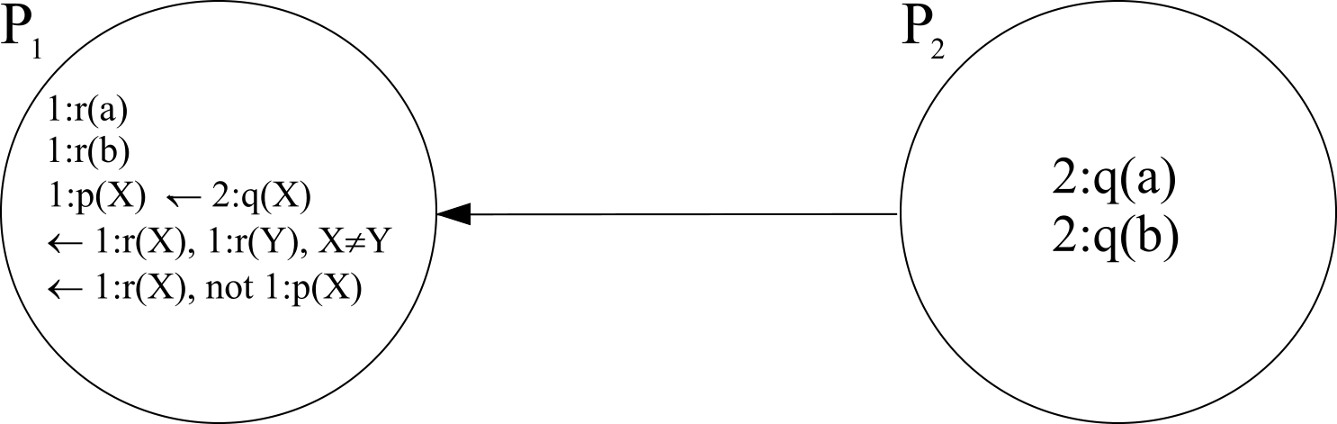
Consider the P2P system in Fig. 8.

The epistemic semantics proposed in [25, 24] states that both atoms and are imported in peer which becomes inconsistent. In this case the semantics assumes that the whole P2P system is inconsistent and every atom is true as it belongs to all minimal models. Consequently, and are true. The semantics proposed in [41] assumes that only is inconsistent as it has no model. Thus, as the atoms and are true in (they belong to all models of ) and the atoms and can be derived in . Finally, and are true. The Maximal weak model semantics, here proposed, states that with and being true in , either or could be imported in (but not both, otherwise the integrity constraint is violated) and, consequently, only one tuple is imported in the relation of the peer . Note that, whatever is the derivation in , is derived in while is not derived. Therefore, the atoms and are, respectively, true and false in . Considering Example 2, as the peer is inconsistent the semantics presented in [25, 24] cut it off from the system, whereas our semantics restore consistency in by importing either or .
In all previous proposals mapping rules are of ‘import kind’. None of them uses mapping rules to fix the knowledge of a correct, but incomplete database as we do by means of minimal mapping rules. They all adopt the traditional classical idea of importing knowledge and use mapping rules as logical implications. In this paper, we follow a different perspective. Maximal mapping rules are used by a peer to import as much knowledge as possible, while preventing inconsistencies, whereas minimal mapping rules are used by a peer as a means to restore consistency by importing minimal sets of data. Moreover, the combined use of both maximal and minimal mapping rules allows to characterize each peer in the neighborhood as a resource used either to enrich (integrate) or to fix (repair) the knowledge, so as to define a kind of integrate-repair strategy. This feature has no counterpart in the above mentioned proposals.
Preferences in P2P Data Management Systems.
In a more general perspective, interesting semantics for data exchange systems, that offer the possibility of explicitly modeling some preference criteria while performing the data integration process, has been proposed in [10, 11, 12, 29, 30]. In [10, 11, 12] a semantics is proposed that allows for cooperation among pairwise peers that are related to each other by means of data exchange constraints (i.e. mapping rules) and trust relationships. The decision by a peer on what other data to consider (besides its local data) does not depend only on its data exchange constraints, but also on the trust relationship that it has with other peers. Given a peer in a P2P system a solution for is a database instance that respects the exchange constraints and trust relationship has with its ‘immediate neighbors’. Trust relationships are of the form: stating that trusts itself less that , stating that trusts itself more that and stating that trusts itself the same as . These trust relationships are static and are used in the process of collecting data in order to establish preferences in the case of conflicting information.
The introduction of preference criteria among peers is out of the scope of this paper, and in the present proposal no explicit preference is formally defined. In any case, note that, an implicit preference is embedded into maximal and minimal mapping rules. Specifically, maximal mapping rules state that it is preferable to import as long as no local inconsistencies arise; whereas minimal mapping rules state that it is preferable not to import unless a local inconsistency exists. In addition, a second implicit level of preference exists in our proposal. Each peer trusts more local data over imported data, therefore our framework always gives more preference to local data over data imported by external peers. This setting can be easily modified in order to cope with the different perspectives in which a generic peer trusts less or the same its own data w.r.t. data provided by external peers.
We have proposed in recent papers extensions of the Max Weak Model Semantics that allow to explicitly express preferences between peers: in [29] a mechanism is defined that allows to set different degrees of reliability for neighbor peers.
More specifically, the paper extends the Max Weak Model Semantics with a mechanism that allows to set priorities among mapping rules. While collecting data it is quite natural for a source peer to associate different degrees of reliability to the portion of data provided by its neighbor peers. Starting from this simple observation, the paper in [29] enhances the Max Weak Model Semantics by using priority levels among mapping rules in order to select the maximal weak models containing a maximum number of mapping atoms according to their importance. Trusted Weak Models can be computed as stable models of a logic program with weak constraints [18, 22].
Both in [29] and in [10, 12] the mechanism is rigid in the sense that the preference among conflicting sets of atoms that a peer can import from only depends on the priorities (trust relationship) fixed at design time.
To overcome static preferences, in [30] ‘dynamic’ preferences, that allow to select among different scenarios looking at the properties of data provided by the peers, is introduced.
The work in [30] allows to model concepts like “in the case of conflicting information, it is preferable to import data from the neighbor peer that
can provide the maximum number of tuples” or “in the case of conflicting information, it is preferable to import data from the neighbor peer such that the sum of the values of an attribute is minimum” without selecting a-priori preferred peers.
Relationship to Multi-Context Systems.
General peer to peer data management systems are related to Multi-Context Systems (MCS). A MCS consists of a set of contexts and a set of inference rules (known as mapping or bridge rules) that allows the information flow between different contexts. The general nonmonotonic MCS model has been defined in [16]. The paper proposes a general framework for multi-context reasoning that enables to combine arbitrary monotonic and nonmonotonic logics. Information flows among contexts by means of nonmonotonic bridge rules and several different notions of equilibrium for acceptable belief have been investigated.
In [37, 38] inconsistencies are analyzed in MCSs, in order to understand where and why they occur and how they can be managed. Each context is assumed to be consistent, therefore the reason of inconsistencies just relies on the application of mapping rules. The paper introduces two approaches of explaining inconsistencies in MCSs in terms of bridge rules: the first notion characterizes inconsistencies in terms of mapping rules that need to be altered to restore consistency, and the second notion looks for combinations of rules which cause inconsistency. The two notions, following the classical terminology in [58], are called respectively diagnosis and explanation.
Using the concept of diagnosis it is possible to capture the semantics of maximal P2P systems
in terms of MCSs. A Multi Context System is a collection of contexts , where , is a logic, is a knowledge base and is a set of bridge rules, for .
An equilibrium is a tuple , where, for , is the knowledge derived from and the heads of the bridge rules in whose bodies are satisfied by .
We consider equilibria that are minimal under component wise set inclusion.77
7
For precise definitions of these concepts see [16]
A diagnosis is a pair , where and are subsets of , such that removing from the bridge rules in and adding to the bridge rules of in inconditional form (obtained from the rules in by removing the bodies), is consistent.
A maximal P2P system , where
, with , can be modeled with a MCS system , where, for , , is
the ASP logic and is obtained by removing the peer identifier from .
One can show that the set of maximal weak models of correspond to the minimal equilibria
of the MCS obtained by removing from the bridge rules of diagnosis of the form , where is minimal.
A P2P system cannot be modeled by an MCS (in its basic form) if it contains minimal mapping rules.
Example 23
Let’s consider the P2P system presented in Example 4. It can be modeled by a MCS
having two ASP contexts, and , where is the ASP logic,
, ,
and . Clearly, is inconsistent because it does not admit any equilibrium. Indeed, the atoms and are derived in , its integrity
constraint is violated and it does not have an acceptable state.
admits two minimal diagnosis of the form .
The first one is . If we remove its bridge rule from , we obtain an MCS having only one minimal equilibrium: . It corresponds to the maximal weak model .
The second one is and removing its bridge rule from , we obtain an MCS having the only minimal equilibrium . It corresponds to the maximal weak model .
As for additional element of discussion, our proposal falls within the area of P2P system,
in which a generic peer is a kind of dynamic context whose presence is not guaranteed in the system, that is a peer may enter and leave the system, arbitrarily. Therefore, the focus in the P2P context (and also in our paper) is not that of finding the
explanations of inconsistencies, but just to cope with them.
Moreover, in our work a generic peer is given the possibility to decide
how to interact with a neighbor peer:
the use of maximal mapping rules states that it is preferable to import as long as no local inconsistencies arise; whereas the use of
minimal mapping rules states that it is preferable not to import unless a local inconsistency exists.
This specific notion has not a counterpart in any of the above works in the field of MCS.
In [13] a fully distributed approach for reasoning in Ambient Intelligent Environments, based on the multi context system paradigm has been proposed.
The paper refers to the propositional case and inconsistencies are managed
by prioritizing mapping rules that cause inconsistency, and specifically
the decision which mapping rule to ignore is based, for every context, on the imposed strict total order of all contexts.
Specifically, the user is forced to establish, at design time, the preference ordering on all the contexts and, as a consequence,
this allow to obtain a unique solution in polynomial time. As for a comparison,
our approach models autonomous logic-based entities (peers) that interchange pieces of information
using mapping rules.
The essential feature of a P2P system is that each peer may leave and join the system arbitrarily. Due to this specific dynamic nature, our proposal avoids forcing any a priori preference ordering and as a consequence may admit many preferred weak models, whose computational complexity is in the second level of the polynomial hierarchy.
In addition the work in [13] does not deal with the case in which the peer is locally inconsistent, whereas we can cope with this issue.
More generally, our proposal supports information flow between different agents through mapping rules, enables reasoning with inconsistent local information (minimal model semantics) and handles agents that provide mutually inconsistent information.
On the other hand, it assumes that all peers share a common alphabet of constants and does not include any notion of privacy.
In addition, the present proposal in its basic framework does not include any notion of preference between
peers, which could be used to resolve potential conflicts caused by mutually inconsistent
information sources and does not provide an algorithm for distributed computation.
These last two features have been already investigated in other works of the same authors and have been briefly discussed in
Section 6.
More specifically, different extensions including preference criteria and aggregate functions have been proposed in [29, 30, 31] and
a distributed computation assigning semantics to a P2P system in polynomial time has been presented in [34, 33].
Context theories can also be modeled as
theories of defeasible logic [4, 55, 56], mappings as defeasible rules and
a preference ordering on the system contexts is used to solve conflicts.
8 Concluding Remarks and Directions for Further Research
In this paper we have proposed three different semantics for P2P deductive databases.
In the Max Weak model Semantics a peer imports maximal sets of atoms from its neighborhood to enrich its knowledge while maintaining inconsistency anomalies.
In the Min Weak model semantics the P2P system can be locally inconsistent, and the information provided by the neighbors is used in order to restore consistency, that is to only integrate with a missing portion of knowledge a correct but incomplete database.
In addition, the present paper unifies the previous two different perspectives captured by the Maximal and Minimal Weak Model Semantics into the Max-Min Weak Model Semantics. This declarative semantics, being more general, allows to characterize each peer in the neighborhood as a resource used either to enrich (integrate) or to fix (repair) the knowledge, so as to define a kind of integrate-repair strategy for each peer in the P2P setting.
The paper also introduces an alternative characterization of the Max-Min Weak Model Semantics (resp. Max Weak Model Semantics and Min Weak Model Semantics) by rewriting a P2P system into an equivalent prioritized logic program. Results on the complexity of answering queries are also presented. The paper, by considering analogous results on stable model semantics for prioritized logic programs, proves that for disjunction-free () prioritized programs deciding whether an interpretation is a max-min weak model of is complete; deciding whether an atom is true in some preferred model is -complete, whereas deciding whether an atom is true in every preferred model is -complete [60]. Moreover, the paper also provides results on the existence of a max-min weak model showing that the problem is in .
Our work opens several avenues for future research. As a direction for further research, the work could be enriched by the introduction of preference criteria and explicit level of trusts so as to allow, in the presence of multiple alternatives, the selection of data satisfying specific criteria and/or provided by the most reliable sources.
References
- Abiteboul and Duschka (1998) Abiteboul, S. and Duschka, O. M. 1998. Complexity of answering queries using materialized views. In Proceedings of the Seventeenth ACM SIGACT-SIGMOD-SIGART Symposium on Principles of Database Systems, June 1-3, 1998, Seattle, Washington, USA. 254–263.
- Abiteboul et al. (1995) Abiteboul, S., Hull, R., and Vianu, V. 1995. Foundations of Databases. Addison-Wesley.
- Adjiman et al. (2006) Adjiman, P., Chatalic, P., Goasdoué, F., Rousset, M., and Simon, L. 2006. Distributed reasoning in a peer-to-peer setting: Application to the semantic web. J. Artif. Intell. Res. 25, 269–314.
- Antoniou and Williams (1997) Antoniou, G. and Williams, M. 1997. Nonmonotonic reasoning. MIT Press.
- Arenas et al. (1999a) Arenas, M., Bertossi, L., and Chomicki, J. 1999a. Consistent query answers in inconsistent databases. In Proceedings of the Eighteenth ACM SIGMOD-SIGACT-SIGART Symposium on Principles of Database Systems. PODS ’99. ACM, New York, NY, USA, 68–79.
- Arenas et al. (1999b) Arenas, M., Bertossi, L. E., and Chomicki, J. 1999b. Consistent query answers in inconsistent databases. In Proceedings of the Eighteenth ACM SIGACT-SIGMOD-SIGART Symposium on Principles of Database Systems, May 31 - June 2, 1999, Philadelphia, Pennsylvania, USA. 68–79.
- Ariew (1976) Ariew, R. 1976. ckham’s razor: A historical and philosophical analysis of ockham’s principle of parsimony.
- Ben-Eliyahu and Dechter (1992) Ben-Eliyahu, R. and Dechter, R. 1992. Propositional sematics for disjunctive logic programs. In Logic Programming, Proceedings of the Joint International Conference and Symposium on Logic Programming, JICSLP 1992, Washington, DC, USA, November 1992. 813–827.
- Bernstein et al. (2002) Bernstein, P. A., Giunchiglia, F., Kementsietsidis, A., Mylopoulos, J., Serafini, L., and Zaihrayeu, I. 2002. Data management for peer-to-peer computing : A vision. In Proceedings of the Fifth International Workshop on the Web and Databases, WebDB 2002, Madison, Wisconsin, USA, June 6-7, 2002, in conjunction with ACM PODS/SIGMOD 2002. Informal proceedings. 89–94.
- Bertossi and Bravo (2004) Bertossi, L. E. and Bravo, L. 2004. Query answering in peer-to-peer data exchange systems. In Current Trends in Database Technology - EDBT 2004 Workshops, EDBT 2004 Workshops PhD, DataX, PIM, P2P&DB, and ClustWeb, Heraklion, Crete, Greece, March 14-18, 2004, Revised Selected Papers. 476–485.
- Bertossi and Bravo (2007) Bertossi, L. E. and Bravo, L. 2007. The semantics of consistency and trust in peer data exchange systems. In Logic for Programming, Artificial Intelligence, and Reasoning, 14th International Conference, LPAR 2007, Yerevan, Armenia, October 15-19, 2007, Proceedings. 107–122.
- Bertossi and Bravo (2017) Bertossi, L. E. and Bravo, L. 2017. Consistency and trust in peer data exchange systems. TPLP 17, 2, 148–204.
- Bikakis et al. (2011) Bikakis, A., Antoniou, G., and Hassapis, P. 2011. Strategies for contextual reasoning with conflicts in ambient intelligence. Knowl. Inf. Syst. 27, 1, 45–84.
- Binas and McIlraith (2008) Binas, A. and McIlraith, S. A. 2008. Peer-to-peer query answering with inconsistent knowledge. In Principles of Knowledge Representation and Reasoning: Proceedings of the Eleventh International Conference, KR 2008, Sydney, Australia, September 16-19, 2008. 329–339.
- Brewka and Eiter (1999) Brewka, G. and Eiter, T. 1999. Preferred answer sets for extended logic programs. Artif. Intell. 109, 1-2, 297–356.
- Brewka and Eiter (2007) Brewka, G. and Eiter, T. 2007. Equilibria in Heterogeneous Nonmonotonic Multi-Context Systems. In Robert C. Holte and Adele Howe, editors, 22nd AAAI Conference on Artificial Intelligence (AAAI’07), AAAI Press, 2007. 1-2, 385–390.
- Brewka et al. (2003) Brewka, G., Niemelä, I., and Truszczynski, M. 2003. Answer set optimization. In IJCAI-03, Proceedings of the Eighteenth International Joint Conference on Artificial Intelligence, Acapulco, Mexico, August 9-15, 2003. 867–872.
- Buccafurri et al. (2000) Buccafurri, F., Leone, N., and Rullo, P. 2000. Enhancing disjunctive datalog by constraints. IEEE Trans. Knowl. Data Eng. 12, 5, 845–860.
- Calvanese et al. (2005) Calvanese, D., De Giacomo, G., Lembo, D., Lenzerini, M., and Rosati, R. 2005. Inconsistency tolerance in P2P data integration: An epistemic logic approach. In Database Programming Languages, 10th International Symposium, DBPL 2005, Trondheim, Norway, August 28-29, 2005, Revised Selected Papers. 90–105.
- Calì et al. (2004) Calì, A., Calvanese, D., De Giacomo, G., and Lenzerini, M. 2004. Data integration under integrity constraints. Inf. Syst. 29, 2, 147–163.
- Calì et al. (2003) Calì, A., Lembo, D., and Rosati, R. 2003. On the decidability and complexity of query answering over inconsistent and incomplete databases. In Proceedings of the Twenty-Second ACM SIGACT-SIGMOD-SIGART Symposium on Principles of Database Systems, June 9-12, 2003, San Diego, CA, USA. 260–271.
- Calimeri et al. (2006) Calimeri, F., Faber, W., Pfeifer, G., and Leone, N. 2006. Pruning operators for disjunctive logic programming systems. Fundam. Inform. 71, 2-3, 183–214.
- Calvanese et al. (2003) Calvanese, D., Damaggio, E., De Giacomo, G., Lenzerini, M., and Rosati, R. 2003. Semantic data integration in P2P systems. In Databases, Information Systems, and Peer-to-Peer Computing, First International Workshop, DBISP2P, Berlin Germany, September 7-8, 2003, Revised Papers. 77–90.
- Calvanese et al. (2008) Calvanese, D., De Giacomo, G., Lembo, D., Lenzerini, M., and Rosati, R. 2008. Inconsistency tolerance in P2P data integration: An epistemic logic approach. Inf. Syst. 33, 4-5, 360–384.
- Calvanese et al. (2004) Calvanese, D., De Giacomo, G., Lenzerini, M., and Rosati, R. 2004. Logical foundations of peer-to-peer data integration. In Proceedings of the Twenty-third ACM SIGACT-SIGMOD-SIGART Symposium on Principles of Database Systems, June 14-16, 2004, Paris, France. 241–251.
- Caroprese et al. (2006) Caroprese, L., Greco, S., and Zumpano, E. 2006. A logic programming approach to querying and integrating P2P deductive databases. In Proceedings of the Nineteenth International Florida Artificial Intelligence Research Society Conference, Melbourne Beach, Florida, USA, May 11-13, 2006. 31–36.
- Caroprese et al. (2006) Caroprese, L., Molinaro, C., and Zumpano, E. 2006. Integrating and querying P2P deductive databases. In Tenth International Database Engineering and Applications Symposium (IDEAS 2006), 11-14 December 2006, Delhi, India. 285–290.
- Caroprese and Zumpano (2007) Caroprese, L. and Zumpano, E. 2007. Consistent data integration in P2P deductive databases. In Scalable Uncertainty Management, First International Conference, SUM 2007, Washington, DC, USA, October 10-12, 2007, Proceedings. 230–243.
- Caroprese and Zumpano (2008) Caroprese, L. and Zumpano, E. 2008. Modeling cooperation in P2P data management systems. In Foundations of Intelligent Systems, 17th International Symposium, ISMIS 2008, Toronto, Canada, May 20-23, 2008, Proceedings. 225–235.
- Caroprese and Zumpano (2011) Caroprese, L. and Zumpano, E. 2011. Aggregates and priorities in P2P data management systems. In 15th International Database Engineering and Applications Symposium (IDEAS 2011), September 21 - 27, 2011, Lisbon, Portugal. 1–7.
- Caroprese and Zumpano (2012a) Caroprese, L. and Zumpano, E. 2012a. Handling preferences in P2P systems. In Foundations of Information and Knowledge Systems - 7th International Symposium, FoIKS 2012, Kiel, Germany, March 5-9, 2012. Proceedings. 91–106.
- Caroprese and Zumpano (2012b) Caroprese, L. and Zumpano, E. 2012b. Restoring consistency in P2P deductive databases. In Scalable Uncertainty Management - 6th International Conference, SUM 2012, Marburg, Germany, September 17-19, 2012. Proceedings. 168–179.
- Caroprese and Zumpano (2017a) Caroprese, L. and Zumpano, E. 2017a. P2P deductive databases: a system prototype. In Proceedings of the 19th International Conference on Information Integration and Web-based Applications & Services, iiWAS 2017, Salzburg, Austria, December 4-6, 2017. 258–265.
- Caroprese and Zumpano (2017b) Caroprese, L. and Zumpano, E. 2017b. P2P deductive databases: Well founded semantics and distributed computation. In New Trends in Databases and Information Systems - ADBIS 2017 Short Papers and Workshops, AMSD, BigNovelTI, DAS, SW4CH, DC, Nicosia, Cyprus, September 24-27, 2017, Proceedings. 91–99.
- Chatalic et al. (2006) Chatalic, P., Nguyen, G. H., and Rousset, M. 2006. Reasoning with inconsistencies in propositional peer-to-peer inference systems. In ECAI 2006, 17th European Conference on Artificial Intelligence, August 29 - September 1, 2006, Riva del Garda, Italy, Including Prestigious Applications of Intelligent Systems (PAIS 2006), Proceedings. 352–356.
- Delgrande et al. (2003) Delgrande, J. P., Schaub, T., and Tompits, H. 2003. A framework for compiling preferences in logic programs. TPLP 3, 2, 129–187.
- Eiter et al. (2010) Eiter, T., Fink, M., Schüller, P., and Weinzierl, A. 2010. Finding explanations of inconsistency in multi-context systems. In Principles of Knowledge Representation and Reasoning: Proceedings of the Twelfth International Conference, KR 2010, Toronto, Ontario, Canada, May 9-13, 2010.
- Eiter et al. (2014) Eiter, T., Fink, M., Schüller, P., and Weinzierl, A. 2014. Finding explanations of inconsistency in multi-context systems. Artif. Intell. 216, 233–274.
- Fagin et al. (2005) Fagin, R., Kolaitis, P. G., Miller, R. J., and Popa, L. 2005. Data exchange: semantics and query answering. Theor. Comput. Sci. 336, 1, 89–124.
- Fagin et al. (2005) Fagin, R., Kolaitis, P. G., and Popa, L. 2005. Data exchange: getting to the core. ACM Trans. Database Syst. 30, 1, 174–210.
- Franconi et al. (2003) Franconi, E., Kuper, G. M., Lopatenko, A., and Serafini, L. 2003. A robust logical and computational characterisation of peer-to-peer database systems. In Databases, Information Systems, and Peer-to-Peer Computing, First International Workshop, DBISP2P, Berlin Germany, September 7-8, 2003, Revised Papers. 64–76.
- Franconi et al. (2004a) Franconi, E., Kuper, G. M., Lopatenko, A., and Zaihrayeu, I. 2004a. A distributed algorithm for robust data sharing and updates in P2P database networks. In Current Trends in Database Technology - EDBT 2004 Workshops, EDBT 2004 Workshops PhD, DataX, PIM, P2P&DB, and ClustWeb, Heraklion, Crete, Greece, March 14-18, 2004, Revised Selected Papers. 446–455.
- Franconi et al. (2004b) Franconi, E., Kuper, G. M., Lopatenko, A., and Zaihrayeu, I. 2004b. Queries and updates in the codb peer to peer database system. In (e)Proceedings of the Thirtieth International Conference on Very Large Data Bases, Toronto, Canada, August 31 - September 3 2004. 1277–1280.
- Fuxman et al. (2006) Fuxman, A., Kolaitis, P. G., Miller, R. J., and Tan, W. C. 2006. Peer data exchange. ACM Trans. Database Syst. 31, 4, 1454–1498.
- Gelder (1989) Gelder, A. V. 1989. The alternating fixpoint of logic programs with negation. In Proceedings of the Eighth ACM SIGACT-SIGMOD-SIGART Symposium on Principles of Database Systems, March 29-31, 1989, Philadelphia, Pennsylvania, USA. 1–10.
- Gelfond and Lifschitz (1988) Gelfond, M. and Lifschitz, V. 1988. The stable model semantics for logic programming. In Logic Programming, Proceedings of the Fifth International Conference and Symposium, Seattle, Washington, August 15-19, 1988 (2 Volumes). 1070–1080.
- Greco et al. (2003) Greco, G., Greco, S., and Zumpano, E. 2003. A logical framework for querying and repairing inconsistent databases. IEEE Trans. Knowl. Data Eng. 15, 6, 1389–1408.
- Gribble et al. (2001) Gribble, S. D., Halevy, A. Y., Ives, Z. G., Rodrig, M., and Suciu, D. 2001. What can database do for peer-to-peer? In Proceedings of the Fourth International Workshop on the Web and Databases, WebDB 2001, Santa Barbara, California, USA, May 24-25, 2001, in conjunction with ACM PODS/SIGMOD 2001. Informal proceedings. 31–36.
- Halevy et al. (2003) Halevy, A. Y., Ives, Z. G., Suciu, D., and Tatarinov, I. 2003. Schema mediation in peer data management systems. In Proceedings of the 19th International Conference on Data Engineering, March 5-8, 2003, Bangalore, India. 505–516.
- Halevy et al. (2005) Halevy, A. Y., Ives, Z. G., Suciu, D., and Tatarinov, I. 2005. Schema mediation for large-scale semantic data sharing. VLDB J. 14, 1, 68–83.
- Lenzerini (2002) Lenzerini, M. 2002. Data integration: A theoretical perspective. In Proceedings of the Twenty-first ACM SIGACT-SIGMOD-SIGART Symposium on Principles of Database Systems, June 3-5, Madison, Wisconsin, USA. 233–246.
- Leone et al. (2005) Leone, N., Greco, G., Ianni, G., Lio, V., Terracina, G., Eiter, T., Faber, W., Fink, M., Gottlob, G., Rosati, R., Lembo, D., Lenzerini, M., Ruzzi, M., Kalka, E., Nowicki, B., and Staniszkis, W. 2005. The INFOMIX system for advanced integration of incomplete and inconsistent data. In Proceedings of the ACM SIGMOD International Conference on Management of Data, Baltimore, Maryland, USA, June 14-16, 2005. 915–917.
- Lonc and Truszczynski (2000) Lonc, Z. and Truszczynski, M. 2000. On the problem of computing the well-founded semantics. In Computational Logic - CL 2000, First International Conference, London, UK, 24-28 July, 2000, Proceedings. 673–687.
- Madhavan and Halevy (2003) Madhavan, J. and Halevy, A. Y. 2003. Composing mappings among data sources. In VLDB 2003, Proceedings of 29th International Conference on Very Large Data Bases, September 9-12, 2003, Berlin, Germany. 572–583.
- Marek and Truszczynski (1993) Marek, V. W. and Truszczynski, M. 1993. Nonmonotonic logic - context-dependent reasoning. Artificial intelligence. Springer.
- Nute (1994) Nute, D. 1994. Defeasible logic. In Handbook of logic in artificial intelligence and logic programming, volume 3: Nonmonotonic reasoning and uncertain reasoning, pages 353–395. Oxford University Press.
- Papadimitriou (1994) Papadimitriou, C. H. 1994. Computational complexity. Addison-Wesley.
- Reiter (1987) Reiter, R. 1987. A theory of diagnosis from first principles. Artif. Intell. 32, 1, 57–95.
- Rousset et al. (2006) Rousset, M., Adjiman, P., Chatalic, P., Goasdoué, F., and Simon, L. 2006. SomeWhere: A Scalable Peer-to-Peer Infrastructure for Querying Distributed Ontologies. In On the Move to Meaningful Internet Systems 2006: CoopIS, DOA, GADA, and ODBASE, OTM Confederated International Conferences, CoopIS, DOA, GADA, and ODBASE 2006, Montpellier, France, October 29 - November 3, 2006. Proceedings, Part I.
- Sakama and Inoue (2000) Sakama, C. and Inoue, K. 2000. Prioritized logic programming and its application to commonsense reasoning. Artif. Intell. 123, 1-2, 185–222.
- Tatarinov and Halevy (2004) Tatarinov, I. and Halevy, A. Y. 2004. Efficient query reformulation in peer-data management systems. In Proceedings of the ACM SIGMOD International Conference on Management of Data, Paris, France, June 13-18, 2004. 539–550.