Model reconstruction from temporal data for coupled oscillator networks
Abstract
In a complex system, the interactions between individual agents often lead to emergent collective behavior like spontaneous synchronization, swarming, and pattern formation. The topology of the network of interactions can have a dramatic influence over those dynamics. In many studies, researchers start with a specific model for both the intrinsic dynamics of each agent and the interaction network, and attempt to learn about the dynamics that can be observed in the model. Here we consider the inverse problem: given the dynamics of a system, can one learn about the underlying network? We investigate arbitrary networks of coupled phase-oscillators whose dynamics are characterized by synchronization. We demonstrate that, given sufficient observational data on the transient evolution of each oscillator, one can use machine learning methods to reconstruct the interaction network and simultaneously identify the parameters of a model for the intrinsic dynamics of the oscillators and their coupling.
Keywords: nonlinear dynamics, phase oscillators, Kuramoto oscillators, network reconstruction, network topology, machine learning, computational methods
1 Introduction
Nature and society brim with systems of coupled oscillators, including pacemaker cells in the heart, insulin-secreting cells in the pancreas, neural networks in the brain, fireflies that synchronize their flashing, chemical reactions, Josephson junctions, power grids, metronomes, and applause in human crowds, to name merely a few [1, 2, 3, 4, 5, 6, 7, 8, 9]. The dynamics of coupled oscillators in complex networks have been studied extensively. In particular, networks of interacting oscillators governed by the seminal Kuramoto model [10, 11, 12] or its variants are known to exhibit a rich variety of behaviors including spontaneous synchronization, phase transitions, and pattern formation [13, 14]. The connections in the network can play a pivotal role in determining these dynamics.
Given oscillators where the governing equations and network topology are known, it is fairly straightforward to explore the dynamics of the system using numerical methods and, in special cases, analytical methods. Unfortunately, in many systems, the topology of the interaction network and the intrinsic oscillator properties can be difficult or impossible to observe directly. Imagine, for example, experimental results that track neuronal cell network or gene regulatory network activity for a large number of oscillators, giving rise to time series data. One might like to infer model information from these time series.
It is crucial to distinguish between functional network connections and structural network connections. Functional connectivity refers to the temporal correlation of the oscillators and is often directly observable. For instance, neurons that fire synchronously are functionally connected. In contrast, structural connectivity, also called network topology, refers to the underlying connections present in the network. For instance, neurons that are connected by synapses or neurotransmitters are structurally connected. In many systems these structural connections can be difficult or impossible to observe.
Network reconstruction is an active area of research [15, 16, 17, 18, 19, 20, 21, 22, 23, 24, 25, 26, 27, 28, 29]. In section 2.2, we review the literature most closely related to our approach. In our work, we solve an inverse problem using observed time series data of the coupled oscillators to reconstruct both the network topology, i.e. the structural network connections, and the intrinsic oscillator dynamics. For the remainder of this paper, when we refer to inferring or reconstructing the model, we mean both of the aforementioned components: network connections and intrinsic oscillator properties.
In this paper, our primary contribution is an algorithm that addresses certain challenges of existing methods mentioned above. One such challenge is that existing methods set up the inverse problem as a linear system that involves many unknown parameters. Consequently, a large amount of time series data is necessary. In contrast, our algorithm results in a system of equations that is smaller, and is nonlinear. We solve these using optimization tools designed for neural networks. As a result, we are able to infer the model with a much smaller amount of data. A second challenge, as mentioned in [21, 17, 28], is that it is typically quite difficult to infer the model for networks that are synchronized. For such networks, we explore what perturbations of the synchronized state are needed to enable accurate inference of the model.
The mathematical setting of our study is oscillator networks composed of limit-cycle oscillators. These are also known as phase oscillators, meaning they are characterized by a single phase variable defined on the circle. We explore four different choices of oscillator models, all of which fall into the general framework for uniformly coupled phase oscillators developed in [30]: the classic Kuramoto model [10]; a Kuramoto-like model with square-wave coupling function; the Kuramoto-Sakaguchi model [31]; and a phase-field reduction of weakly-coupled Hodgkin-Huxley oscillators [32] (see A). We take all networks to be Erdös-Rényi random graphs [33]. We attempt to infer the network topology, the intrinsic frequency of each model oscillator, and the so-called coupling function that specifies the influence of one oscillator on others.
To carry out the model reconstruction, we begin with simulated time series for the oscillator phases and estimated phase velocities. We set up an optimization problem involving the mean squared error for the predicted phase velocities generated by a system of nonlinear differential equations, which can be represented as a convolutional neural network. We then use computational methods designed for neural networks to estimate the optimal parameters, thereby inferring the adjacency matrix for network connectivity, the oscillator coupling strength, the oscillator frequencies, and the Fourier coefficients of the coupling function. This approach is effective for a variety of different networks and model parameters. More specifically, we find that:
- •
Accurate inference of the coupling network, frequencies and coupling functions is possible independent of the model when the system does not synchronize or when sufficient perturbations from synchronization are permitted.
- •
Model reconstruction is possible with a smaller amount of data than previous approaches that set up the problem as a large system of linear equations.
- •
Computational methods designed for neural networks, such as mini-batch gradient-descent implemented in TensorFlow [34], can be used to solve the optimization problem associated with model reconstruction.
- •
Synchronizing networks can be reconstructed using random phase resets or sufficiently large phase perturbations to a small randomly-chosen set of oscillators.
- •
Synchronizing networks can also be reconstructed using perturbations to a sufficiently large fixed subset of oscillators.
The rest of this paper is organized as follows. In section 2 we introduce the Kuramoto model (a standard model for the dynamics of coupled oscillators), set up the inverse problem for reconstruction, and discuss approaches for solving this inverse problem. In section 3 we describe a series of experiments used to test the effectiveness of these reconstruction techniques over a wide range of model parameters. In section 4, we present the results of the aforementioned experiments and discuss perturbation strategies for improving the reconstruction when the system synchronizes. Finally, in section 5, we summarize our primary findings and discuss extensions to our methodology.
2 Models and Methods
The Kuramoto model is a standard model for the dynamics of coupled oscillators. We consider oscillators with phases for , each with an intrinsic frequency . These oscillators are coupled through an interaction network with adjacency matrix , with the entry determining whether oscillators and are coupled. The dynamics of are governed by the equation
| (1) |
Here represents the strength of the coupling between oscillators and , and represents the coupling function. If the coupling function is continuous and periodic, and is piecewise continuous, then it can be represented using a uniformly convergent Fourier series
| (2) |
where the coefficients satisfy for some . Therefore, these coefficients decay to for large and this function can be approximated to arbitrary accuracy using a truncated Fourier series
| (3) |
with sufficiently large . Note that within the model, one can set without loss of generality, using the change of variables .
In Kuramoto’s original formulation [10], the oscillators were globally coupled () with coupling strengths where scales the global coupling strength. He used the coupling function , and showed that, for where is a critical value related to the width of the distribution of intrinsic frequencies, the oscillators begin to synchronize, achieving identical phase velocities with phases distributed around the population mean. Analogous results were obtained later for systems with periodic coupling functions possessing only odd harmonics [30, 11] and arbitrary complex networks [35].
2.1 Simulated data generation
We investigate a method for inferring the parameters of the Kuramoto model for phase oscillators on random graphs with uniform coupling strengths . In our experiments, we focus on undirected Erdős-Rényi graphs, where each possible edge in the network is present with probability of . It is straightforward to extend our approach to arbitrary networks with non-uniform coupling strengths, though this would likely require a larger amount of time series data. The details of our method appear in sections 2.2 and 2.3.
| Parameter | Description | Value | Sweep values |
|---|---|---|---|
| number of oscillators | 10 | ||
| average intrinsic frequency | 1.0 | N/A | |
| standard deviation of intrinsic frequencies | 0.5 | ||
| network connection probability | 0.5 | ||
| coupling function | See A | ||
| dyn_noise | noise in system dynamics | 0 |
| Parameter | Description | Value | Sweep values |
|---|---|---|---|
| duration of each transient | 20 | ||
| sampling time step | 0.1 | N/A | |
| noise | observation noise | 0 | |
| number of transients observed | 10 |
In order to test our method, we generate data according to the following procedure:
- 1.
Generate an Erdős-Rényi network for a fixed connection probability where the nodes represent individual oscillators with natural frequencies sampled from a normal distribution with mean and standard deviation .
- 2.
- 3.
Compute the phases at times with timestep and for where to obtain observations that are evenly spaced in time.
- 4.
Estimate the phase velocities using central differencing in time with Savitsky-Golay filtering [38]. We used a window length of with first degree polynomials.
- 5.
Repeat steps (ii-iv) times with different uniform random initial conditions to obtain sufficient data during the transient evolution of the system.
See tables 1 and 2 for the network parameters and numerical solution parameters used in this procedure.
The aforementioned process is intended to produce simulated data mimicking that which experimentalists might collect when observing real world networks. Note however, that it may not be possible to control the initial phases in an experiment. We therefore evaluate the reconstruction methods for varying , as well as for cases in which small perturbations are used instead of different initial conditions (see section 4.1).
2.2 Inverse problem formulation
We will formulate a set of equations whose least squares solution can be used to estimate the natural frequencies of each oscillator, the adjacency matrix of the coupling network, the coupling strength , and the coupling function , from observed phases and phase velocities generated using the method outlined above. This work builds on prior work by Shandilya and Timme [17], where the adjacency matrix for a network of oscillators is estimated from a time series. We summarize their approach below.
Define vectors and consisting of the oscillator phases and phase velocities. When the coupling strength and coupling function are known, the phase velocity for oscillator ,
| (4) |
is linear in the unknown parameters and . Therefore, one can infer both the natural frequencies and adjacency matrix by solving a linear system of equations, where is the number of time steps and each timestep provides equations of the form
| (5) |
Here is an matrix where each row is determined from (4) for a particular oscillator, and is an vector with the unknown natural frequencies and the entries in the adjacency matrix . The number of unknowns in can be reduced to if one assumes and .
Since the number of equations in the linear system is determined by the number of observed timesteps and the number of oscillators , one can ensure that the system is over-determined by collecting enough observations so that . One can then estimate the parameters by minimizing a loss function such as the mean squared error,
where denotes the observed value and denotes the predicted value of the velocity.
As long as the system remains far from synchronization, increasing the number of observations will provide additional linearly independent equations to aid with reconstruction. However, as networks synchronize, i.e. , additional observations become (nearly) linearly dependent. This causes the system of equations to become highly ill-conditioned and makes numerical solutions sensitive to noise and rounding errors. As a result, it is often necessary to perturb the system away from equilibrium to ensure that a sufficient number of linearly independent observations can be collected.
Although the approach of [17] outlined above is effective, it is limited by the requirement that the coupling function be known a priori. In [28], Pikovsky addresses this limitation by expressing as a Fourier series so that it, too, can be estimated by solving an analogous optimization problem. However, a challenge remains. If one represents the coupling function as in (3), then the system of equations is no longer linear as terms of the form and appear. Pikovsky [28] circumvents this issue by defining distinct coupling functions
for each pair of oscillators and by setting . In this formulation, if oscillators and are uncoupled, then for all . This modification preserves the linearity of the system of equations and allows for the description of a more general class of networks with distinct coupling functions for each pair of oscillators. Unfortunately, it comes at a cost: the number of unknown parameters increases dramatically from to . Therefore, even longer observation times are required. Additionally, as with the method of [17], if the system synchronizes, there may be numerical difficulties when inferring parameters. Finally, the large number of free parameters makes this model particularly prone to overfitting. As before, one could assume that connections in the network are symmetric, i.e., that and that self edges are not included , allowing for a reduction in the number of parameters to .
We propose an alternative approach. We use a single coupling function represented by a Fourier series as described in (3) for all coupling terms and attempt to infer the Fourier coefficients and along with the intrinsic frequencies , adjacency matrix , and global coupling strength . This leads to a total inferred parameters or with symmetry constraints and no self-connections. This is therefore a modest increase of parameters over the case considered by Shandilya and Timme [17] without requiring prior knowledge of the coupling function.
As mentioned previously, this leads to a set of nonlinear equations due to the appearance of terms of the form and in (4). Since always appears in products involving and , these parameters are not structurally identifiable. One could set without loss of generality. Instead, we include as an inferred parameter and introduce penalty terms to the objective function we seek to minimize:
| (6) | |||||
The inclusion of a penalty function ensures the existence of a non-degenerate local minimum. In this objective function, the first term above represents the mean squared error. The remaining terms are penalty terms with weights , , and . These hyper-parameter values were tuned initially to provide satisfactory reconstruction performance, and then kept constant in all subsequent experiments (see also table 3). Additional tuning of these parameters for specific networks could further improve the accuracy of the model reconstruction. The second term with introduces regularization which favors smaller estimates of the parameter values and . This is useful for combating overfitting and promoting sparse representations, and is analogous to using a Bayesian prior centered at 0 for the Fourier coefficients [39]. The last term with and penalizes adjacency values that are far from 0 and 1 as well as those that are negative or greater than 1 to ensure that the estimates fall within the desired range of . We do not penalize and instead allow it to be as large as necessary to counteract the parameter shrinkage caused by the penalty terms.
2.3 Inverse problem solution
Minimizing (6) poses a number of challenges. First of all, due to the nonlinearity of (4), this function may not be convex and there are no guarantees that local optimization methods will converge to a global minimum. Secondly, when the number of observations is large, this function may be costly to compute, and minimizing the number of function evaluations is paramount.
Fortunately, the theoretical challenge of nonconvexity does not prevent our method from obtaining consistently reliable model reconstruction, as we show in section 4. The computational difficulties can be addressed by using tools designed for neural networks and implemented in TensorFlow to efficiently compute gradients and perform minimization with a variant of mini-batch gradient descent [40].
To elucidate the connection with neural networks, we comment that (3) can be viewed as a 2-d convolutional neural network with a convolution of size and stride 1 applied to the tensor consisting of phase differences . The hidden layer consists of the harmonics of the form and applied to each entry in this tensor. To avoid redundant weights, we fix the weights in the first hidden layer to be 1 and the biases to be 0. In the second hidden layer, each harmonic is assigned a fixed bias of 0 and a variable weight or corresponding to the Fourier coefficients. Figure 1 provides a schematic of this neural network. Once the coupling terms have been computed, the rest of (4) and the resulting loss function (6) are straightforward to compute using vectorized operations.

We initialize the inferred parameters as follows: the adjacency matrix has initial entries drawn from , the frequencies are initialized from , the coupling strength is drawn from , and the Fourier coefficients of the coupling function are initialized at .
TensorFlow maintains a computational graph for these operations which allows one to automatically compute gradients. One can therefore use gradient descent methods to compute the optimal estimates (,,,,) for the parameters. We used a mini-batch gradient descent method with batch size of , i.e., we randomly assign the data to batches of 100 time-steps. For each batch we calculate the gradient of the loss function and update the estimated parameters by taking a small step in a direction determined from the gradient. Once this has been repeated for all batches (one epoch), we pass through the data again for a total of or more epochs. We determined the number of epochs experimentally by iterating until the mean squared error no longer decreased. Typically, 300 epochs were sufficient. However for certain sweeps examining the role of , , and , the number of epochs required for convergence was as high as 10000.
By using small random batches of time steps, the gradient can be estimated quickly. This has the added benefit of introducing stochasticity into gradients which makes the algorithm less susceptible to getting caught in local minima. We use AdamOptimizer, which is a gradient descent method with momentum and an adaptive learning rate [41], with default parameter values for optimization in TensorFlow.
| Parameter | Description | Value |
|---|---|---|
| n_epochs | iterations through the training data | 300 |
| batch size | time-steps of data per gradient descent batch | 100 |
| number of inferred Fourier coefficients | 5 | |
| weight of penalty on non-sparse coupling | 0.0001 | |
| weight of penalty on network connectivity | ||
| weight of penalty on |
There is minor variability in the success of the algorithm due to the random initialization of the inferred parameters and to the batching of the observed data. In order to ensure an accurate network reconstruction, we can retrain the model with new initial values several times and choose the result which has the smallest mean squared error for the velocity predictions on the validation set, which was not considered during the training process. For any individual model network, this validation error is correlated with the accuracy of the inferred parameters. In all examples below, we attempt to reconstruct each network five times before choosing the best reconstruction.
2.4 Post-processing
The method described in section 2.3 produces continuous estimates for the parameters (,,,,) which could be used to predict the dynamics of the system under a variety of initial conditions. However, we are interested in evaluating whether these parameter estimates are an accurate reconstruction of the original model. Before these values can be compared to the model parameters used to generate the data, additional post-processing is needed. We therefore redefine our parameter estimates via the transformations , where and are selected to minimize , and These transformation are necessary to address the aforementioned identifiability issues with and to allow to have nonzero mean.
In the original model, the adjacency matrix entries are either zero or one. However, we treat the entries as continuous variables during optimization and then choose a threshold so that is chosen to be 0 and is chosen to be 1. In practice, one could fix or select so that the reconstructed model minimizes the mean squared error for the data set. However, we explore a range of threshold values using ROC curves and report the reconstruction error rates using the value of that yields the largest score for the adjacency matrix reconstruction (see B). These optimal values are robust and good performance is typically obtained over a wide range of thresholds (see section 4 for details).
3 Experimental design
In order to validate the robustness of our approach, we test the reconstruction method on data simulated with a variety of networks and parameter values. We explore this high-dimensional parameter space by fixing all of the model parameters except for one and then sweeping the remaining parameter over a wide range of values. See tables 1 and 2 for a list of default values as well as the ranges considered. For each set of parameter values, we compute 30 networks with random initial phases and intrinsic frequencies. We then attempt to reconstruct the underlying model for each network and compute various performance metrics for each reconstruction.
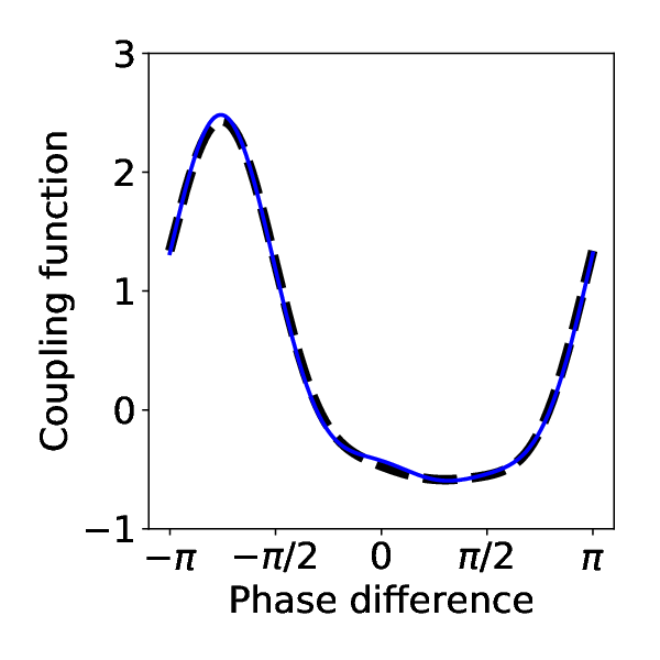
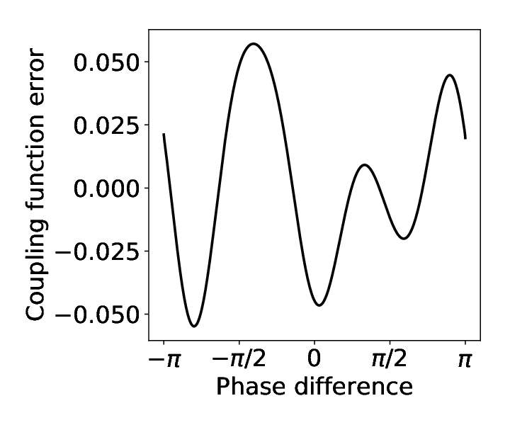
Coupling function — We evaluate the inferred coupling function by comparing it to the true coupling function via the normalized difference in area defined as follows:
| (7) |
This represents the area between the true and estimated coupling function curves, weighted by the area under the curve of the true function. This quantity serves as a measure of the error in the reconstruction. A perfect reconstruction would have a normalized difference in area of zero. In the Kuramoto case , the initial estimate corresponds to a value of 1. Therefore values significantly lower than 1 indicate progress towards a correct reconstruction.
Intrinsic Frequencies — We compare the inferred intrinsic frequencies to the true intrinsic frequencies using the mean absolute deviation defined as follows:
| (8) |
Values near zero indicate accurate reconstructions. We considered alternative metrics such as relative deviations and the correlation between true and inferred frequencies, but these were less informative because they tend to amplify errors when the the intrinsic frequencies are close to zero.



Adjacency matrix — We investigate several methods for evaluating the success of adjacency matrix reconstruction. The accuracy can be inspected visually by plotting the true and reconstructed matrices along with the absolute differences in a grid where values range from (black) to (white); see figure 2(a-c). Since we are primarily interested in discrete adjacency values, we interpret reconstruction as a classification problem and compute three standard evaluation metrics: the score, the classification error rate for the connections, and the area under the ROC curve. See B for precise definitions of these metrics.
4 Results


Here we discuss the key results from the parameter sweeps outlined in section 3.
Our method can successfully reconstruct models with a variety of coupling functions. Figure 3a and table 5 show the results for four different coupling functions (see A for details), three of which come from popular coupled oscillator models: the Kuramoto model, the Kuramoto-Sakaguchi model, and a phase reduction of the Hodgkin-Huxley model, and a fourth, a square wave which represents a generic discontinuous function with high frequency Fourier harmonics. We note that for the square wave coupling function, the accuracy of the reconstruction suffers since the reconstruction includes only five Fourier harmonics and the true coupling function contains an infinite number of harmonics with amplitudes that decay slowly due to the discontinuities. Despite these limitations, the adjacency matrix was still estimated with a high degree of accuracy.
Counterintuitively, as the number of oscillators increases (figure 3b and table 6), we find that reconstruction accuracy improves. This can be explained by the observation that although increasing the number of oscillators increases the number of unknown parameters, it also provides a greater number of pairwise phase differences which can aid in reconstruction of the coupling function. The resulting modest improvements in the estimate of the coupling function can then allow for better inference of the adjacency matrix and intrinsic frequencies as well. This is illustrated by the normalized difference in area plot in figure 3b.
In figure 4 and table 7, we consider simulations where the standard deviation of the oscillator frequencies ranges from to . The normalized difference in area of the coupling function and the mean absolute deviation of the inferred frequencies both show that we can infer the network well for . For larger standard deviations, the quality of the reconstruction suffers slightly, since the large frequencies dominate the coupling terms within the phase velocity relationship.


We also explore the impact of noise on the model reconstruction since both observation noise and dynamic noise would be present in experiments. In table 8 and table 9, we demonstrate that our model reconstruction method is robust to moderate amounts of both types of noise. As in [17], we introduce dynamic noise using stochastic differential equations with Gaussian noise. Observation noise was also Gaussian and was added after integrating the governing differential equations. For both types of noise, we used mean and standard deviations between and . It is worth noting that dynamic noise with a standard deviation less than helps with the reconstruction of both coupling function and frequencies. This can be explained by the fact that a small amount of noise keeps the system from reaching equilibrium, effectively increasing the duration of the transients that provide useful information about the structure of the network.
We carry out additional parameter sweeps with varying network connectivity (table 10), maximum simulation time (table 11) and the number of simulation restarts (table 12) with all other parameters set using the default values given in tables 1, 2, and 3. In each case, we are consistently able to reconstruct the coupling function, the underlying network and the intrinsic frequencies model over a wide range of model parameters. The tables in C illustrate averaged numerical results for 30 trials of each of these parameter sweeps in terms of evaluation metrics such as normalized difference in area, mean absolute deviation, error rate, area under ROC curve, and a range of thresholds that yield scores within of the largest value.
4.1 Results for perturbations of synchronous dynamics
As both [17] and [28] point out, when a network remains synchronized, i.e. when , one cannot infer the model parameters due to the fact that the observed phases no longer provide linearly independent equations. Furthermore, even with precise knowledge of the adjacency matrix, one could not hope to reconstruct the coupling function without data over a wide range of phase differences .
As such we investigated a method for using small perturbations to introduce brief transients into the dynamics to allow for successful model reconstruction. To test this, we used nearly identical oscillators with frequency standard deviation , which causes the system to quickly converge to a synchronized state for almost all initial conditions. We then initialized so that the system begins from perfect synchrony. Then, at times for we added a phase perturbation to a subset of the oscillators. Each perturbation causes some of the oscillators to briefly become desynchronized. In this way, the total number of observed phases remains constant, but the fraction of those observations that occur during transient dynamics is proportional to the number of perturbations, . The observed phases during these transients provide meaningful data about the structure of the network. Figure 6 demonstrates that, as expected, with too few or too small perturbations, model reconstruction is unsuccessful. However, as the number of perturbations increases, the accuracy of the estimated coupling function, adjacency matrix, and the oscillator frequencies improves.


We explored two methods for selecting which oscillators to perturb: fixed subsets, in which the subset of perturbed oscillators was selected at the beginning of the experiment and these same oscillators were perturbed repeatedly, and random subsets, in which a random subset of the system was selected for each perturbation. Although a perturbation to the phase of a particular oscillator does propagate to the phases of neighboring oscillators through the coupling terms, those perturbations decay quickly and are therefore most effective for revealing the local structure of the network. As such, although perturbations to a fixed subset might be more practical in a physical experiment, one must typically perturb a larger fraction of the system to obtain comparable performance to that which is obtained with perturbations to random subsets.
We also considered two types of phase perturbations: phase resets, in which selected oscillators had their phases reset to 0, and phase shifts, in which selected oscillators had their phases modified by adding a random shift . Phase resets may be more feasible from an experimental perspective, but have the drawback of preserving the mutual synchrony of the subset of oscillators that are perturbed. As such one will typically need to use random subsets in tandem with phase resets in order to be able to resolve the connections between the perturbed oscillators.
In figure 6(a-c), we used phase shifts with to a fixed subset of size 1, i.e. a single oscillator out of . This gives poor reconstruction regardless of the number of perturbations due to the small size of the perturbation. On the other hand, in figure 6(d-f) we perturb a fixed subset (3 out of 10 oscillators) with random phase shifts with 11 1 This is virtually indistinguishable from uniform perturbations . In this case, the perturbations affect a sufficiently large proportion of the oscillators and performance begins to improve once there are 5 or more perturbations. The results in figure 6(g-i) illustrate that one only needs to perturb 1 out of 10 oscillators to obtain similar performance when the oscillators selected are chosen randomly. In figure 6(j-l), we show the results using phase resets to random subsets of 3 oscillators. Again, performance begins to improve dramatically once 5 or more perturbations are used. The tables summarizing the results of these perturbation strategies are provided in C.
4.2 Comparison with reference [28]
The amount of transient data necessary for reconstruction is also useful in comparing our method to previous approaches. As discussed in section 2.2, Pikovsky proposes an alternative method where distinct coupling functions are considered for the interaction of each pair of oscillators [28]. This ensures that the system of equations in the optimization is linear, however it also increases the number of unknown coefficients significantly. Our approach relies on the assumption that the same coupling function is used for all pairs of oscillators. This is a reasonable approximation for physical systems when the physical mechanisms governing the interactions between oscillators are the same. Pikovsky [28] uses a more general model in which the coupling functions may be different for each pair of oscillators.


Figure 7 shows that when the coupling functions are identical, our method provides more accurate reconstructions of both the network topology and the coupling function with smaller amounts of transient data. As the amount of transient data increases, both methods ultimately achieve perfect network reconstruction while the approach in [28] ultimately obtains slightly better estimates for the coupling function. Therefore, our approach would be preferred under circumstances where the amount of data is limited and when the coupling functions are nearly identical.
5 Discussion and conclusions
In this paper, we have designed a method for reconstructing models of coupled oscillator networks including both the network connections and the intrinsic oscillator properties. We hope analysts might investigate (non)convexity of our penalty function and properties of minimizers. These issues aside, after testing our method with many different parameters, we conclude that our algorithm can successfully infer the model.
A common challenge that our method and many related ones encounter is that the procedure fails if the system synchronizes too quickly. One remedy is to have a sufficient number of observations during the desynchronized transients. As we demonstrate, one can ensure that this data is available by repeating experiments with multiple initial conditions or by adjusting the model parameters to inhibit synchronization by instituting large frequency variability () or dynamic noise. An alternative remedy is to move the system away from synchrony using perturbations, preferably ones that are physically realizable. The introduction of these perturbations provides useful transient data. By perturbing a sufficiently large subset of oscillators with a large enough change, we are able to infer the model accurately. Our hope is that this method will be adopted by experimentalists and used with experimental data to aid with the construction of interpretable models for the dynamics of networks of coupled oscillators.
Although the numerical experiments outlined here involve Erdös-Rényi networks, the method can be applied more generally to a broad class of networks. Preliminary testing suggests that similar results can be obtained for other topologies such as star, small-world, scale-free networks, and clique networks.
It is also straightforward to extend this approach to other models for coupled phase oscillators such as the Winfree model [42] or even more general oscillator models such as the Stuart-Landau model [43] in which both phase and amplitude variations are permitted. Indeed, any system where the unknown functions are periodic can be represented using our technique.
For models containing unknown functions that are not periodic such as the Hodgkin-Huxley model [44], a Fourier series representation is not possible. In these cases, one could represent the coupling functions using feed-forward neural networks, which are capable of representing continuous functions to arbitrary accuracy using a finite number of parameters [45]. Given a sufficiently rich data set, one could still use our approach with back-propagation to learn the structure of the neural network approximation for the coupling function.
Appendix A Coupling functions
The coupling functions investigated are described in table 4. The first three classes of functions were selected due to their use in popular coupled oscillator models. The last was an example of a generic coupling function with higher order harmonics that was tested to verify that reconstruction of the adjacency matrix is possible even with an imperfect approximation to the coupling function.
Appendix B Evaluation metrics for classification
The score is defined as
Here, is the fraction of true positives among all inferred positives, while is the fraction of true positives among all positives. The score is a value between and ; when reporting the error rate for the reconstructed adjacency matrix, we use the threshold that corresponds to the largest score. We also determine the interval of thresholds that yield scores within 90% of this largest value. The width of this interval is reported in the tables in C as “Interval width ”.
The error rate is defined as the percentage of entries in that are incorrectly classified. We report the error rate for the optimal threshold discussed in section 2.4.
The ROC curve, or receiver operating characteristic, is a parametric curve that uses the classification threshold as a parameter and uses the true positive rate and the false positive rate as the the variables [46]. The area under the ROC curve measures the quality of a classifier independent any particular threshold. A value of is consistent with blind guesses, and a value of indicates a perfect classifier since it implies the existence of a threshold for which the rate of true positives is and the rate of false positives is . Our ROC curves were generated using the scikit-learn package in Python [47].
Appendix C Tables of results
Here we include several tables which report the averaged numerical results of the experimental parameter sweeps described in section 3 and reported on in section 4. The performance metrics used are defined in B. Values given in the tables represent the mean plus or minus one standard deviation of the corresponding performance metric over the 30 trials run at that parameter value. We note that some of the distributions, such as the error rate (which is nonnegative by definition), are skewed.
| Param | Value |
|
|
Error rate |
|
| ||||||||
|---|---|---|---|---|---|---|---|---|---|---|---|---|---|---|
| Kuramoto | 0.0175 0.0075 | 0.004 0.001 | 0.0 0.0 | 1.0 0.0 | 0.4338 | |||||||||
| Kuramoto-Sakaguchi | 0.0169 0.0054 | 0.005 0.002 | 0.0 0.0 | 1.0 0.0 | 0.3924 | |||||||||
| Hodgkin-Huxley | 0.0343 0.0159 | 0.011 0.004 | 0.0 0.0 | 1.0 0.0 | 0.7054 | |||||||||
| Square wave | 0.1518 0.0044 | 0.006 0.002 | 0.0 0.0 | 1.0 0.0 | 0.4059 |
| Param | Value |
|
|
Error rate |
|
| ||||||||
|---|---|---|---|---|---|---|---|---|---|---|---|---|---|---|
| 5 | 0.026 0.0125 | 0.0052 0.003 | 0.0 0.0 | 1.0 0.0 | 0.1193 | |||||||||
| 10 | 0.0164 0.007 | 0.0047 0.0031 | 0.0 0.0 | 1.0 0.0 | 0.4057 | |||||||||
| 20 | 0.015 0.0057 | 0.0046 0.0016 | 0.140 0.601 | 0.9997 0.0016 | 0.3041 | |||||||||
| 40 | 0.0189 0.0104 | 0.0045 0.0011 | 1.231 1.018 | 0.9946 0.0053 | 0.223 |
| Param | Value |
|
|
Error rate |
|
| ||||||||
|---|---|---|---|---|---|---|---|---|---|---|---|---|---|---|
| 0.01 | 0.0198 0.0052 | 0.0022 0.0008 | 0.0 0.0 | 1.0 0.0 | 0.8142 | |||||||||
| 0.1 | 0.0175 0.0057 | 0.004 0.0014 | 0.0 0.0 | 1.0 0.0 | 0.8095 | |||||||||
| 1 | 0.0161 0.0049 | 0.0042 0.0021 | 0.0 0.0 | 1.0 0.0 | 0.7975 |
| Param | Value |
|
|
Error rate |
|
| ||||||||
|---|---|---|---|---|---|---|---|---|---|---|---|---|---|---|
| noise | 0 | 0.0193 0.0098 | 0.0048 0.002 | 0.0 0.0 | 1.0 0.0 | 0.4204 | ||||||||
| noise | 1e-05 | 0.0202 0.0108 | 0.0053 0.0024 | 0.0 0.0 | 1.0 0.0 | 0.3845 | ||||||||
| noise | 0.0001 | 0.018 0.0076 | 0.0048 0.0023 | 0.0 0.0 | 1.0 0.0 | 0.4365 | ||||||||
| noise | 0.001 | 0.0186 0.0081 | 0.0053 0.002 | 0.0 0.0 | 1.0 0.0 | 0.3956 | ||||||||
| noise | 0.01 | 0.0186 0.0079 | 0.0052 0.0025 | 0.0 0.0 | 1.0 0.0 | 0.4135 | ||||||||
| noise | 0.1 | 0.0385 0.0138 | 0.0086 0.0021 | 0.0 0.0 | 1.0 0.0 | 0.3544 | ||||||||
| noise | 1 | 0.831 0.1343 | 0.118 0.0629 | 46.296 8.579 | 0.5122 0.0741 | 0.0472 |
| Param | Value |
|
|
Error rate |
|
| ||||||||
|---|---|---|---|---|---|---|---|---|---|---|---|---|---|---|
| dyn_noise | 0 | 0.0211 0.0067 | 0.0055 0.0018 | 0.0 0.0 | 1.0 0.0 | 0.3814 | ||||||||
| dyn_noise | 1e-05 | 0.0117 0.0069 | 0.0032 0.0023 | 0.0 0.0 | 1.0 0.0 | 0.4048 | ||||||||
| dyn_noise | 0.0001 | 0.0146 0.0049 | 0.0032 0.0013 | 0.0 0.0 | 1.0 0.0 | 0.411 | ||||||||
| dyn_noise | 0.001 | 0.0241 0.0056 | 0.0049 0.0017 | 0.0 0.0 | 1.0 0.0 | 0.4517 | ||||||||
| dyn_noise | 0.01 | 0.0633 0.0189 | 0.0128 0.0034 | 0.370 1.025 | 0.9982 0.0072 | 0.3282 | ||||||||
| dyn_noise | 0.1 | 0.2136 0.065 | 0.0312 0.0055 | 14.148 5.003 | 0.8903 0.0496 | 0.2224 | ||||||||
| dyn_noise | 1 | 0.9716 0.0399 | 0.1552 0.0971 | 42.444 8.953 | 0.5177 0.1004 | 0.0406 |
| Param | Value |
|
|
Error rate |
|
| ||||||||
|---|---|---|---|---|---|---|---|---|---|---|---|---|---|---|
| 0.1 | 0.1199 0.2314 | 0.0054 0.0047 | 3.111 14.97 | 0.9688 0.1548 | 0.3387 | |||||||||
| 0.2 | 0.023 0.0098 | 0.004 0.0022 | 0.074 0.41 | 0.9999 0.0006 | 0.5222 | |||||||||
| 0.3 | 0.0186 0.0073 | 0.0047 0.0025 | 0.0 0.0 | 1.0 0.0 | 0.5175 | |||||||||
| 0.4 | 0.0207 0.0089 | 0.0047 0.0022 | 0.0 0.0 | 1.0 0.0 | 0.5167 | |||||||||
| 0.5 | 0.0189 0.0097 | 0.0051 0.0024 | 0.0 0.0 | 1.0 0.0 | 0.4669 | |||||||||
| 0.6 | 0.0183 0.0072 | 0.006 0.0019 | 0.0 0.0 | 1.0 0.0 | 0.349 | |||||||||
| 0.7 | 0.0169 0.0071 | 0.005 0.0025 | 0.0 0.0 | 1.0 0.0 | 0.3227 | |||||||||
| 0.8 | 0.0194 0.0077 | 0.0057 0.0026 | 0.0 0.0 | 1.0 0.0 | 0.2725 | |||||||||
| 0.9 | 0.0289 0.0271 | 0.0077 0.0056 | 0.0 0.0 | 1.0 0.0 | 0.2739 |
| Param | Value |
|
|
Error rate |
|
| ||||||||
|---|---|---|---|---|---|---|---|---|---|---|---|---|---|---|
| 2 | 0.0204 0.011 | 0.0042 0.002 | 0.0 0.0 | 1.0 0.0 | 0.8225 | |||||||||
| 5 | 0.0185 0.0064 | 0.0047 0.0022 | 0.0 0.0 | 1.0 0.0 | 0.8186 | |||||||||
| 10 | 0.0193 0.0066 | 0.004 0.0013 | 0.0 0.0 | 1.0 0.0 | 0.8175 | |||||||||
| 20 | 0.0192 0.0053 | 0.0041 0.0013 | 0.0 0.0 | 1.0 0.0 | 0.565 | |||||||||
| 50 | 0.0191 0.0093 | 0.0064 0.0038 | 0.0 0.0 | 1.0 0.0 | 0.2964 |
| Param | Value |
|
|
Error rate |
|
| ||||||||
|---|---|---|---|---|---|---|---|---|---|---|---|---|---|---|
| 1 | 0.0513 0.0266 | 0.0237 0.0127 | 3.111 3.531 | 0.9815 0.027 | 0.447 | |||||||||
| 2 | 0.0343 0.0222 | 0.0082 0.007 | 0.148 0.564 | 0.9986 0.0067 | 0.6943 | |||||||||
| 5 | 0.019 0.0094 | 0.0039 0.002 | 0.0 0.0 | 1.0 0.0 | 0.806 | |||||||||
| 10 | 0.0201 0.0084 | 0.0042 0.0028 | 0.0 0.0 | 1.0 0.0 | 0.808 | |||||||||
| 20 | 0.018 0.0033 | 0.0042 0.0017 | 0.0 0.0 | 1.0 0.0 | 0.8295 | |||||||||
| 40 | 0.0192 0.0055 | 0.0041 0.0016 | 0.0 0.0 | 1.0 0.0 | 0.8178 |
| Param | Value |
|
|
Error rate |
|
| ||||||||
|---|---|---|---|---|---|---|---|---|---|---|---|---|---|---|
| 1 | 0.9318 0.082 | 0.118 0.0719 | 48.667 7.459 | 0.2934 0.0999 | 0.0252 | |||||||||
| 2 | 0.9054 0.1176 | 0.3284 0.0747 | 49.778 6.920 | 0.2904 0.0783 | 0.0306 | |||||||||
| 5 | 0.7928 0.1568 | 0.3853 0.1243 | 51.852 8.702 | 0.3281 0.0895 | 0.0688 | |||||||||
| 10 | 0.7828 0.1698 | 0.2566 0.1579 | 50.593 5.110 | 0.3843 0.0697 | 0.1403 | |||||||||
| 20 | 0.9818 0.0083 | 0.0024 0.0011 | 43.630 9.383 | 0.5153 0.0959 | 0.1026 | |||||||||
| 40 | 0.931 0.0234 | 0.0019 0.0007 | 47.556 9.403 | 0.4909 0.0935 | 0.0931 |
| Param | Value |
|
|
Error rate |
|
| ||||||||
|---|---|---|---|---|---|---|---|---|---|---|---|---|---|---|
| 1 | 0.9193 0.1111 | 0.1161 0.0643 | 49.778 7.042 | 0.3189 0.1051 | 0.0298 | |||||||||
| 2 | 0.7919 0.2112 | 0.343 0.0724 | 49.852 6.331 | 0.279 0.0949 | 0.0409 | |||||||||
| 5 | 0.4298 0.1535 | 0.3328 0.0691 | 39.778 11.032 | 0.5271 0.1261 | 0.2041 | |||||||||
| 10 | 0.3211 0.1187 | 0.1697 0.0769 | 22.741 10.975 | 0.7388 0.0974 | 0.2111 | |||||||||
| 20 | 0.1311 0.0931 | 0.0288 0.0302 | 4.667 5.296 | 0.9536 0.0601 | 0.3584 | |||||||||
| 40 | 0.0447 0.0311 | 0.0036 0.0026 | 0.222 0.679 | 0.9988 0.0057 | 0.4824 |
| Param | Value |
|
|
Error rate |
|
| ||||||||
|---|---|---|---|---|---|---|---|---|---|---|---|---|---|---|
| 1 | 0.8851 0.1332 | 0.1203 0.0716 | 50.0 5.277 | 0.316 0.1035 | 0.0293 | |||||||||
| 2 | 0.7678 0.215 | 0.2857 0.0916 | 50.963 6.879 | 0.315 0.0915 | 0.0326 | |||||||||
| 5 | 0.286 0.0821 | 0.1973 0.0625 | 30.963 9.096 | 0.6136 0.1118 | 0.1767 | |||||||||
| 10 | 0.1567 0.0624 | 0.0788 0.0609 | 15.704 4.246 | 0.7659 0.0863 | 0.3186 | |||||||||
| 20 | 0.0783 0.056 | 0.0268 0.06 | 10.815 4.943 | 0.8699 0.0777 | 0.4238 | |||||||||
| 40 | 0.0262 0.0191 | 0.0041 0.0078 | 7.185 4.837 | 0.9391 0.0565 | 0.5419 |
| Param | Value |
|
|
Error rate |
|
| ||||||||
|---|---|---|---|---|---|---|---|---|---|---|---|---|---|---|
| 1 | 0.891 0.1231 | 0.1058 0.0706 | 46.889 8.444 | 0.3337 0.1156 | 0.0299 | |||||||||
| 2 | 0.9214 0.088 | 0.3684 0.0897 | 50.444 7.031 | 0.2938 0.0783 | 0.0474 | |||||||||
| 5 | 0.2075 0.0319 | 0.0313 0.0179 | 23.704 10.379 | 0.7769 0.0874 | 0.2803 | |||||||||
| 10 | 0.0294 0.0061 | 0.0033 0.0014 | 1.926 2.592 | 0.9894 0.0157 | 0.3855 | |||||||||
| 20 | 0.0184 0.003 | 0.0015 0.0007 | 0.074 0.406 | 0.9999 0.0008 | 0.522 | |||||||||
| 40 | 0.0116 0.0028 | 0.0015 0.0005 | 0.0 0.0 | 1.0 0.0 | 0.6206 |
| Param | Value |
|
|
Error rate |
|
| ||||||||
|---|---|---|---|---|---|---|---|---|---|---|---|---|---|---|
| 1 | 0.8188 0.1236 | 8633.13 25993.8 | 45.852 8.159 | 0.5239 0.0886 | 2012.5215 | |||||||||
| 2 | 0.8895 0.2663 | 3481.08 9497.15 | 23.037 11.635 | 0.7415 0.1298 | 1.6593 | |||||||||
| 5 | 0.2267 0.3482 | 2.5746 11.3136 | 2.148 7.063 | 0.9756 0.0733 | 0.75 | |||||||||
| 10 | 0.0238 0.0242 | 0.0061 0.0078 | 0.074 0.406 | 0.9979 0.0114 | 0.8436 | |||||||||
| 20 | 0.0099 0.0037 | 0.0024 0.001 | 0.0 0.0 | 1.0 0.0 | 0.9131 | |||||||||
| 40 | 0.0077 0.0033 | 0.0023 0.001 | 0.0 0.0 | 1.0 0.0 | 0.9329 |
References
- [1] Trautwein W and Kassebaum D G 1961 J. Gen. Phys. 45 317–330
- [2] Stagner J I, Samols E and Weir G C 1980 J. Clin. Invest. 65 939–942
- [3] Buzsaki G and Draguhn A 2004 Science 304 1926–1929
- [4] Buck J 1988 Q. Rev. Biol. 63 265–289
- [5] Tinsley M R, Nkomo S and Showalter K 2012 Nat. Phys. 8 662–665
- [6] Hadley P, Beasley M and Wiesenfeld K 1988 Phys. Rev. B 38 8712–8719
- [7] Motter A E, Myers S A, Anghel M and Nishikawa T 2013 Nat. Phys. 9 191–197
- [8] Pantaleone J 2002 Am. J. Phys. 70 992–1000
- [9] Néda Z, Ravasz E, Vicsek T, Brechet Y and Barabási A L 2000 Phys. Rev. E 61 6987–6992
- [10] Kuramoto Y 1975 Self-entrainment of a population of coupled non-linear oscillators International symposium on mathematical problems in theoretical physics (Springer) pp 420–422
- [11] Acebron J A, Bonilla L L, Perez Vicente C J, Ritort F and Spigler R 2005 Rev. Mod. Phys. 77(1) 137–185
- [12] Arenas A, Diaz-Guilera A, Kurths J, Moreno Y and Zhou C 2008 Phys. Rep. 469 93–153
- [13] Strogatz S H 2000 Physica D 143 1–20
- [14] Panaggio M J and Abrams D M 2015 Nonlinearity 28 R67–R87
- [15] Wang W X, Chen Q, Huang L, Lai Y C and Harrison M A F 2009 Phys. Rev. E 80(1) 016116
- [16] Ta H X, Yoon C N, Holm L and Han S K 2010 BMC Syst. Biol. 4 70
- [17] Shandilya S G and Timme M 2011 New J. Phys. 13 013004
- [18] Ching E S C, Lai P Y and Leung C Y 2013 Phys. Rev. E 88(4) 042817
- [19] Ching E S C, Lai P Y and Leung C Y 2015 Phys. Rev. E 91(3) 030801
- [20] Lin W, Wang Y, Ying H, Lai Y C and Wang X 2015 Phys. Rev. E 92(1) 012912
- [21] Timme M and J C 2014 J. Phys. A: Math. Theor. 47 343001
- [22] Tirabassi G, Sevilla-Escoboza R, Buldú J M and Masoller C 2015 Scientific reports 5 10829
- [23] Tirabassi G, Sevilla-Escoboza R, Buldu J M and Masoller C 2015 Sci. Rep. 5 10829
- [24] Bianco-Martinez E, Rubido N, Antonopoulos C G and Baptista M 2016 Chaos 26 043102
- [25] Alderisio F, Fiore G and di Bernardo M 2017 Phys. Rev. E 95(4) 042302
- [26] Angulo M T, Moreno J A, Lippner G, Barabási A L and Liu Y Y 2017 J. Roy. Soc. Int. 14
- [27] Stolz B J, Harrington H A and Porter M A 2017 Chaos 27 047410
- [28] Pikovsky A 2018 Phys. Lett. A 382 147–152
- [29] Leguia M G, Levnajic Z, Todorovski L and Zenko B 2019 1–22 (Preprint arXiv/1902.03896)
- [30] Daido H 1992 Prog. Theor. Phys. 88 1213–1218
- [31] Sakaguchi H and Kuramoto Y 1986 Prog. Theor. Phys. 76 576–581
- [32] Hansel D, Mato G and Meunier C 1993 Europhys. Lett. 23 367
- [33] Erdős P and Rényi A 1960 Publ. Math. Inst. Hung. Acad. Sci 5 17–60
- [34] Abadi M, Agarwal A, Barham P, Brevdo E, Chen Z, Citro C, Corrado G S, Davis A, Dean J, Devin M, Ghemawat S, Goodfellow I, Harp A, Irving G, Isard M, Jia Y, Jozefowicz R, Kaiser L, Kudlur M, Levenberg J, Mané D, Monga R, Moore S, Murray D, Olah C, Schuster M, Shlens J, Steiner B, Sutskever I, Talwar K, Tucker P, Vanhoucke V, Vasudevan V, Viégas F, Vinyals O, Warden P, Wattenberg M, Wicke M, Yu Y and Zheng X 2015 TensorFlow: Large-scale machine learning on heterogeneous systems software available from tensorflow.org URL https://www.tensorflow.org/
- [35] Rodrigues F A, Peron T K D, Ji P and Kurths J 2016 Phys. Rep. 610 1 – 98 ISSN 0370-1573 the Kuramoto model in complex networks
- [36] Dormand J and Prince P 1980 Journal of Computational and Applied Mathematics 6 19 – 26 ISSN 0377-0427
- [37] Honeycutt R L 1992 Phys. Rev. A 45(2) 600–603
- [38] Savitzky A and Golay M J 1964 Analytical chemistry 36 1627–1639
- [39] Murphy K P 2012 Machine learning: a probabilistic perspective (MIT press)
- [40] Panaggio M J, Ciocanel M V and Lazarus L 2019 Coupled oscillator network modelreconstruction https://github.com/mpanaggio/coupled_oscillator_network_model_reconstruction/tree/published
- [41] Kingma D P and Ba J 2014 (Preprint arXiv:1412.6980)
- [42] Winfree A T 2001 The geometry of biological time vol 12 (Springer Science & Business Media)
- [43] Nakagawa N and Kuramoto Y 1993 Progress of Theoretical Physics 89 313–323
- [44] Hodgkin A L and Huxley A F 1952 The Journal of physiology 117 500–544
- [45] Hornik K 1991 Neural Netw. 4 251 – 257
- [46] Fawcett T 2006 Pattern Recognit. Lett. 27 861–874
- [47] Pedregosa F, Varoquaux G, Gramfort A, Michel V, Thirion B, Grisel O, Blondel M, Prettenhofer P, Weiss R, Dubourg V, Vanderplas J, Passos A, Cournapeau D, Brucher M, Perrot M and Duchesnay E 2011 J. Mach. Learn. Res 12 2825–2830