Numerical study of the negative nonlocal resistance and the backflow current in a ballistic graphene system
Abstract
Besides the giant peak of the nonlocal resistance , an anomalous negative value of has been observed in graphene systems, while its formation mechanism is not quite understood yet. In this work, utilizing the non-equilibrium Green’s function method, we calculate the local-current flow in an H-shaped non-interacting graphene system locating in the ballistic regime. Similar to the previous conclusions made from the viscous hydrodynamics, the numerical results show that a local-current vortex appears between the nonlocal measuring terminals, which induces a backflow current and a remarkable negative voltage drop at the probe. Specifically, the stronger the vortex exhibits, the more negative manifests. Besides, a spin-orbital coupling is added as an additional tool to study this exotic vortex, which is not a driving force for the arising vortex at all. Moreover, a breakdown of the nonlocal Wiedemann-Franz law is obtained in this ballistic system, and two experimental criteria are further provided to confirm the existence of this exotic vortex. Notably, a discussion is made that the vortex actually originates from the collision between the flowing current and the boundaries, due to the long electron mean free path and the consequent ballistic transport caused by the specific linear spectrum of graphene.
pacs
71.70.Ej, 72.10.-d, 73.23.-bI Introduction
Nonlocal measurement indicates the detection of a voltage signal away from the path that the current is expected to follow, and has been developed as a powerful tool to discover nontrivial interactions difficult to detect directly, such as the electron-electron () interaction, viscosity, spin-orbital coupling, etc Huber; Abanin1; Balakrishnan; Nowack; Gorbachev; Shimazaki; Sui; Michihisa; Bandurin1; Bandurin2; Braem; Wu; Berdyugin. Besides the giant peak of the nonlocal resistance , more and more experiments have observed an anomalous negative value of the nonlocal resistance Bandurin1; Bandurin2; Berdyugin, which means the local current close to the nonlocal terminals flows in direction opposite to the injected current. Till now, kinds of theories have been proposed to explain this exotic phenomenon, such as the viscous hydrodynamic fluidBandurin1; Levitov; Alekseev; Levin, the ballistic transportWang; Tuan; Shytov; Chandra, the magnetoelectric couplingHuang and so on.
Among these theories, viscous hydrodynamics is the most developed one Bandurin1; Levitov; Alekseev; Levin, and has been supported by the recent experiments for a two-dimensional fluid of electrons in grapheneBerdyugin; Gallagher. The condition for viscous hydrodynamics happens when the extrinsic scattering length is far greater than the collision mean free path . That is to say, electrons injected into the system must undergo frequent collisions with each other inside the bulk, which can be well described by the theory of hydrodynamics Jong; Scaffidi; Lucas. For instance, Bandurin et al. detected an anomalous nonlocal negative voltage drop in a multi-terminal graphene device on the order of Bandurin1. By solving the hydrodynamic equations, a submicrometer-size whirlpool in the electron flow can be obtained. Moreover, the calculation results show that the whirlpool enhances with the increase of the viscosity, and disappears with zero viscosity, which fits the experiment well. Thus, this negative nonlocal resistance is attributed to the formation of a local-current vortex.
More comprehensively, some literatures further propose that in the interaction dominated but quasi-ballistic regime, where is much smaller than , the negative value of the nonlocal resistance can occur as wellShytov; Bandurin2; Braem. Furthermore, as a direct prove to the ballistic transport without collision, our previous work and others based on the non-equilibrium Green’s function (NEGF) method predict that the ballistic transport itself could induce a negative nonlocal resistance Wang; Tuan. In addition, with the help of the semi-classical Boltzmann equation and phenomenological conditions, recent work could even obtain a vortex in the ballistic regime classicallyChandra. However, compared with the well-studied theory in hydrodynamics, the formation mechanism of the negative observed in ballistic system without interaction desperately needs in-depth analysis, such as the demonstration of the local-current flow in the view of quantum transport.
In this work, we further study the origin of the negative nonlocal resistance in a non-interacting graphene model with an external Rashba effect, and try to confirm whether the local-current vortex also exists in this ballistic system, similar as that in a viscous fluidBandurin1. First, in an H-shaped four-terminal graphene system, we calculate the local-current distribution with different Fermi energy and different Rashba strength . The results show that an exotic vortex emerges between the two nonlocal measuring terminals similar to that in a viscous fluid. Further calculation indicates that this vortex strengthens with the decrease of . In comparison with the fact that the negative value of the nonlocal resistance also increases with weakening Rashba effect, we confirm that the vortex has a positive relation to the negative nonlocal resistance. Thus, a conclusion can be made that the ballistic transport in the nonlocal measurement does exist in the form of a vortex, which consists of backflow current and induces a negative contribution to the nonlocal resistance. Then, the local and nonlocal thermal conductance of this system are also obtained within the NEGF framework. In comparison to the scaled local (nonlocal) electrical conductance (), we find that our ballistic system actually breaks the nonlocal Wiedemann-Franz (WF) law instead of the local one found in hydrodynamicsCrossno, and this violation gradually disappears with weakening vortex strength. Based on the above results, we further propose two experimental methods to confirm the existence of the local-current vortex in a ballistic system. Specifically, with increasing , both the negative value of and the breakdown of the nonlocal WF law should gradually disappear in ballistic regime. At last, a discussion is made that it is actually the collision between the flowing current and the boundaries that induces this exotic vortex. Since this collision highly relies on a long electron mean free path and the consequent ballistic transport, the vortex will be much easier to be observed in graphene due to its unique linear energy dispersion.
The rest of this paper is organized as follows. In Sec.II, we first numerically obtain the local-current flow and find a vortex in an H-shaped four-terminal ballistic graphene system. Then, in Sec.III, we propose two experimentally feasible methods to confirm the existence of this vortex indirectly in the ballistic regime. Next, a discussion about the possible origin of the vortex flow is made in Sec.IV. And finally, a conclusion is presented in Sec.V.
II Local-current flow in H-shaped four-terminal system

In this work, we consider an H-shaped four-terminal graphene systemfoot1, whose schematic diagram is shown in Fig.1(a), to simulate the local current distribution in the nonlocal measuring experiment. The central region for this system is marked with parameters and . For instance, in Fig.1, we show a sample with and . During the calculation process, the current is injected from lead 1 and flows out from lead 2. Meanwhile, the nonlocal voltage is detected between lead 3 and 4. In this paper, we only show the local current distributed in the rectangle region, which is surrounded by the black dashed line. This is due to the fact that we find the local-current flow exhibits nontrivial characteristics only between the nonlocal measuring terminals, and exhibits the classical Ohmic distribution in other regions.
Similar as our previous work of Ref.[Wang], the tight-binding Hamiltonian for this system is written as:
| (1) |
The first term is the on-site potential with on the th carbon atom. The second term represents the nearest-neighbor hopping with strength . In the following calculation, we take as the energy unit and all other parameters are normalized based on eV. The last term describes the external Rashba effect with strength . The disorder existing in the central region is modeled by Anderson disorder with random potential uniformly distributed in , where is the disorder strength. In this work, we choose .

In Ref.[Wang], we have specifically introduced how to calculate the local and the nonlocal resistance: and based on the Landauer-Buttiker formulabook. Since it’s the local-current distribution that we focus on in this work, the size of the central region is limited for the convenience and clearness to read the local-current flow vectors inside the black dashed line. Thus, the size parameters , , and are chosen as , , and , which means the size of this system we calculated is about foot2.
In order to simulate the local-current flow in the nonlocal measuring experiment, a small external voltage bias is applied between lead 1 and 2. With the help of the NEGF method, the local current flows from site to its neighbor can be deduced asJauho; Jiang:
| (2) |
where , denote the spin indices, and is the Keldysh Green’s function. When the applied voltage is small and the system is in the zero temperature, by applying the Keldysh equation and assuming , the Eq.(2) can be rewritten as:
| (3) | |||||
where is the voltage of the th lead, and can be obtained in the calculation of . is the electron correlation function. The linewidth function is , and the Green’s function reads . Here, is the retarded self-energy due to the coupling to the th lead, and is the Hamiltonian used in the central region. The first part of Eq.(3) gives rise to the equilibrium current , which equals zero due to the time-reversal symmetry of the Hamiltonian described by Eq.(1). Thus, the local current flows from site to its neighbor can be simplified as:
| (4) |
Moreover, based on Eq.(4), the current flowing from lead to the central region can be obtained by summing over all the local current at the boundary between lead and the central region. In comparison with acquired from the previous calculation of and , we can further testify the correctness of Eq.(4) and the accuracy of our calculation program.
In Fig.2, we first show the spatial distributions of the local current inside the black dashed rectangle marked in Fig.1, when the Rashba effect is fixed at . Throughout this work, we only discuss the negative part of the Fermi energy for simplicity, and the conclusion for positive is the same. From Fig.2(a) to 2(c), the Fermi energy locates at , and , respectively. Here, the size and the orientation of the arrows indicate the strength and the direction of the local-current flow.
As shown in Fig.2(a), it is obvious that there exists a counter-clockwise vortex of the local current between the two nonlocal measuring terminalsfoot3, which seems like the whirlpools obtained in viscous hydrodynamic systems. Importantly, the appearance of this vortex induces a kind of backflow current flowing from lead 4 to lead 3, which is in the direction opposite to the injected current. Consequently, there exists a competition between the positive voltage drop caused by the Ohmic transport and the negative one caused by the backflow current. Thus, it is natural for us to anticipate that if the “vortex strength”foot4 is strong enough, a negative voltage drop between and will be detected, and a negative nonlocal resistance will be obtained consequently as people have shown in previous work.


Moreover, from Fig.2(a) to 2(c), we find that the strength of the vortex reaches its maximum at , then weakens gradually with the increase of the Fermi energy, and finally disappears when the Fermi energy is large enough. In order to confirm the relationship between the vortex of the local current and the appearance of the negative , in Fig.3(a), we show how and vary with the Fermi energy when the Rashba effect is fixed at . The macroscopic oscillations come from the resonance in the Fabry-Pérot cavity, because the size of our system is very small. As a contrast, in Fig.3(c) and 3(d), we show the result with a system twice the size of that in Fig.3(a) and 3(b), where the oscillations become relatively negligible now. Notably, in Fig.3(c) and 3(d), we find the whole shape of vs shrinks along the axis and the negative peak move towards the original point. Since the Rashba effect always appears in the form of during the calculation, the shrink of indicates that a smaller is needed with a larger system size, which is more practical in experiments. In Fig.3(a), it is obvious that the blue lines of exhibits a giant peak near the Dirac point, then decays rapidly to its negative maximum at about , and finally approaches zero as the absolute value of continues to increase. The giant peak of has been discussed in our previous workWang, which is assumed resulting from the extremely small density of states at the Dirac point, and has no relationship to the vortex in our system. Thus, in order to eliminate this effect, we only consider the region where throughout this work. As expected, by comparing Fig.2 and Fig.3(a), the most negative locates exactly where the strongest vortex emerges, and the negative value of decreases as the vortex disappears gradually. Thus, we can make a conclusion that the negative value of originates from the vortex emerging between the nonlocal measuring terminals. The stronger the vortex exhibits, the more negative manifests.
Another method to further study the relationship between the negative value of and the strength of the vortex is to alter the Rashba strength while remains unchanged. In Fig.3(b), we show how varies with under three different Rashba strengths , 0.15 and 0.2. As one can see, apart from the region close to the Dirac point, the negative value of decreases with increasing . This phenomenon can be understood as follows: if the Rashba effect is extremely strong, the current injected into lead 1 will first transport to lead 3 along the upper edge of the system due to the spin Hall effect, then undergoes collisions with the boundary of the system, and finally flows from lead 3 to lead 4. As above, the Rashba effect actually makes a positive contribution to the nonlocal resistance , which is in consistent with our previous calculation of shown in Ref.[Wang]. However, since the Rashba effect and the vortex always coexist with each other in reality, the local-current flow induced by the Rashba effect will eliminate the strength of the vortex caused by the ballistic transport in a certain degree. Consequently, the vortex should gradually disappear as the Rashba effect strengthens.
Following this line of reasoning, in Fig.4, we show the spatial distributions of the local current inside the black dashed rectangle marked in Fig.1, when the Fermi energy is fixed at . From Fig.4(a) to 4(c), the strength of the Rashba effect increases from to and . As expected before, the vortex exhibits most obviously at , and gradually disappears with the increase of . Now, based on the calculation of the local-current flow, we demonstrate that the ballistic transport proposed in previous works indeed gives rise to a vortex in the local-current distribution, which further induces backflow current in the direction opposite to the injected current and results in the negative observed both in theory and experiment. Specifically, the stronger the vortex is, the more negative exhibits.
III Two experimental criteria to the existence of the backflow current
Interestingly, the backflow current induced by the vortex shown in Fig.2 and 4 has also been obtained theoretically in graphene system dominated by interactionBandurin1; Levitov. To be specific, although the Hamiltonian of Eq.(1) has no terms of interaction and locates at the ballistic regime, both our system and the dominated one described by viscous hydrodynamics exhibit similar properties: the negative value of and the backflow current. Significantly, in hydrodynamic theories, the vortex strength highly depends on the viscosity magnitude, and the vortex disappears with zero viscosity. In contrast, for our ballistic system, according to Fig.4, the vortex strength decreases with the increasing Rashba effect. Thus, the backflow current and the negative value of proposed in our ballistic system can be controlled by tuning the Rashba strength , which mainly relies on external electric field and can be realized in experiments. Furthermore, since has little relation to the viscosity, we believe that one possible method to distinguish the appearance of the vortex current between the ballistic and the hydrodynamic system is to tune the external electric field in order to alter the extrinsic Rashba strength . Specifically, by increasing the external electric field, a reduction of the negative will be detected in experiment, which indicates the weakening of the backflow current in the ballistic regime. While the hydrodynamic regime is not sensitive to the varying Rashba effect.
In addition, there also exist other signatures for the appearance of backflow current in the ballistic regime. For instance, the breakdown of the nonlocal WF law based on the NEGF calculation. The local and nonlocal thermal conductances are defined as: and , respectively. Here, indicates the temperature of lead and represents the heat current flowing from lead to the central region. Based on the NEGF method, can be calculated asLiu:
| (5) |
where is the Fermi distribution function. And is the transmission coefficient from lead to , which can be obtained during the calculation of and .

In Fig.5(a), we first plot the local thermal conductance alongside at when . For a direct quantitative comparison based on the WF law, the scaled local conductance in the same units as is also shown, where is the Lorenz ratio. It is obvious that these two values coincide with each other when the absolute value of is larger than 0.1. Then, in Fig.5(b), we also show the nonlocal thermal conductance and its corresponding scaled nonlocal conductance . The major difference between Fig.5(a) and 5(b) is that: the latter one exhibits an obviously additional violation of the nonlocal WF law at , while the former one does not. Moreover, in Fig.5(b), is higher than near the Dirac point, and this relationship reverses at . The above phenomena indicate that the physical pictures behind the violations at and must be totally different. Since the vortex only exists between the nonlocal measuring terminals, which affects the nonlocal WF law instead of the local one, it is most likely that the violation at results from this exotic vortex.
In order to further confirm the origin of the violation at , we enlarge the Rashba strength from to 0.2 and 0.3 in Fig.5(c) and 5(d), respectively. It is clear that the nonlocal WF law breakdown at gradually weakens with the increase of , which provides evidence for the claim that this nonlocal WF law violation actually originates from the vortex and its subsequent backflow current. Thus, it is another feasible method in experiments that the appearance of the vortex in ballistic system could be testified indirectly with the nonlocal thermal conductance and the consequent breakdown of the nonlocal WF law. More accurate analysis for the formation mechanism of this violation needs a comparison between the local electrical current flow and local thermal current flow, which is not shown in this work.
Above all, by altering the Rashba spin-orbital interaction strength , two possible experimental methods have been proposed to distinguish the appearance of the local-current vortex in ballistic regime. The first one is to detect the negative value of and its variation with , and the second one is to probe the nonlocal thermal conductance and compared it with the nonlocal WF law.
IV Discussion
In this section, let’s focus on the possible mechanisms to the formation of the exotic vortex. First, the effect of the impurity scattering needs to be clarified in our analysis. For comparison, we also calculate under a weaker disorder strength compared with presented above. However, the calculating results show that with exhibits more negative value than that with . Therefore, the collision between the electrons and the impurities inside actually plays a negative role to the formation of the vortex.
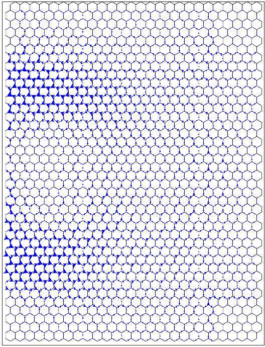
Then, based on the Boltzmann equation, a recently published literature proved that a vortex could also be found in the ballistic regimeChandra. In this semi-classical calculation, the momentum relaxation time is set so small that the system has a sufficient long electron mean free path () and definitely locates in the ballistic regime. Thus, there must exist collisions between the flowing electrons and the boundaries, which seems like the key role to the observation of the vortex. In Fig.6, by adding a list of very strong Anderson disorder at the boundaries of our model, the boundary condition of the specular reflection can be changed to a diffuse one, which loses momentum but keeps energy conservation. As we can see, there still exists a vortex between the nonlocal measuring terminals. The main difference between Fig.6 and 2(a) is that the vortex in Fig.6 tends to move left into the central region. This phenomenon comes from the fact that the net momentum parallel to the boundary becomes zero after the diffuse scattering, while the net perpendicular momentum still exists. Based on the above analysis, we believe that the vortex directly originates from the collisions between the injected current and the boundaries, which is the result of ballistic transport and the corresponding long .

Following the above analysis, the kernel question turns into which condition could guarantee such a long that the system locates in the ballistic regime. In Fig.7, we further calculate the local-current distribution of a square lattice model whose size and Hamiltonian are the same as those of the graphene model used previously. In order to make a better comparison between the graphene and square lattice, the Fermi energy is fixed at , which guarantees locates near the bottom band of the square lattice spectrum. Thus, both the energy and the momentum are nearly the same and consequently comparable between the graphene and the square lattice model.
As shown in Fig.7, though the Rashba strength is chosen as , which is the same as that in Fig.2(a), it is clear that only the classical Ohm-like current could be found and no vortex exists in the square lattice model. This phenomenon comes from the fact that at the small momentum , both the graphene and the square lattice structures have relatively large wavelength. However, since there exists linear spectrum relationship in honeycomb lattice, graphene is delocalized compared with the strong Anderson localization in square lattice. Thus, in square lattice will be much smaller than that in honeycomb lattice. To a certain degree, when of the square lattice decreases to be shorter than the size of the system, there is no ballistic transport, which results in the disappearance of the vortex in square lattice as shown in Fig.7.
To sum up, we can now make a conclusion that the vortex directly results from the elastic or semi-elastic collision between the injected current and the boundaries. However, this collision needs the existence of a sufficient long and the consequent ballistic transport, which highly relies on the linear spectrum of the graphene and the electron delocalization. Thus, it will be much easier for us to obtain a vortex with a relatively pure graphene sample than others.
Finally, the difference between the classical Boltzmann equation and our NEGF method should also be clarified. Specifically, the use of the classical Boltzmann equation needs a sufficient long , which is not calculated microscopically but only considered phenomenologically. That is to say, the establishment of the Boltzmann equation depends on the condition that the system has already located in the ballistic regime, which makes no difference to the honeycomb and square lattices. In contrast, our calculation based on the NEGF method originates from the basic Hamiltonian. And the quantum transport could deal with different values of disorder strength, which is more accurate and helps us better understand the specific differences between the honeycomb and square lattice structures.
V Conclusion
In conclusion, using the NEGF method, we first calculate the local-current flow in an H-shaped noninteracting graphene system locating in the ballistic regime. Interestingly, an obvious vortex, similar to the one appears in a viscous hydrodynamic fluid, can be found between the nonlocal measuring terminals. This vortex strengthens with decreasing of the external Rashba effect, and induces a backflow current in the direction opposite to that of the injected current. These properties highly accord with the confusing negative nonlocal resistance , which has been observed in both experiments and theories previously. The consistency comes from the fact that the backflow current results in a negative voltage drop between the nonlocal measuring terminals, and further induces a competition to the positive one caused by the spin Hall transport. Furthermore, we demonstrate that with enlarging Rashba effect strength, both the vortex and the corresponding negative value of become smaller, and disappear simultaneously when the Rashba effect strength is sufficiently strong. Thus, we conclude that the ballistic transport can also give rise to a vortex, and may serve as a different origin of the observed negative nonlocal , providing an alternative picture to that of the viscous hydrodynamic fluid. We have to emphasize that the above alternative mechanism of the local current vortex does not imply that the previous conclusion obtained from the hydrodynamics is incorrect, but only an important supplement, because the model and the sample size used here are quite different.
Next, we propose two experimental methods to verify the existence of vortex in ballistic regime by tuning the strength of the external Rashba effect : the variations of the negative value of and the breakdown of the nonlocal WF law. Since the interaction dominated system is relatively insensitive to the Rashba effect, these two methods can, in principle, be used to distinguish the physics in the ballistic and viscous systems as well. Moreover, since the vortex always leads to the existence of a magnetic flux, this exotic vortex could also be detected with the newly developed superconducting quantum interference device (SQUID)Kirtley.
Finally and notably, based on a comparison between our graphene system and a square lattice model, a discussion is made that the unique linear spectrum of graphene results in a sufficient long , which makes the system easier to enter into the ballistic regime. Furthermore, the exotic vortex directly originates from this ballistic transport and the consequent collisions between the flowing current and the boundaries.
ACKNOWLEDGMENTS
We thank the insightful discussions with Qing-feng Sun and Jie Liu. This work was financially supported by the Science Challenge Project (SCP) under Grant No. TZ2016003-1, NSFC under Grants Nos. 11704348, 11534001, 11822407, 11674028, and NBRPC under Grants Nos. 2017YFA0303301, 2017YFA0303304.
References
- (1) M. E. Huber, N. C. Koshnick, H. Bluhm, L. J. Archuleta, T. Azua, P. G. Björnsson, B. W. Gardner, S. T. Halloran, E. A. Lucero, and K. A. Moler, Rev. Sci. Instrum 79, 053704 (2008).
- (2) D. A. Abanin, S. V. Morozov, L. A. Ponomarenko, R. V. Gorbachev, A. S. Mayorov, M. I. Katsnelson, K. Watanabe, T. Taniguchi, K. S. Novoselov, L. S. Levitov, and A. K. Geim, Science 332, 328 (2011).
- (3) J. Balakrishnan, G. K. Koon, M. Jaiswal, A. H. Castro Neto, and B. Özyilmaz, Nat. Phys. 9, 284 (2013).
- (4) K. C. Nowack, E. M. Spanton, M. Baenninger, M. König, J. R. Kirtley, B. Kalisky, C. Ames, P. Leubner, C. Brüne, H. Buhmann, L. W. Molenkamp, D. Goldhaber-Gordaon, and K. A. Moler, Nat. Mater. 12, 787 (2013).
- (5) R. V. Gorbachev, J. C. W. Song, G. L. Yu, A. V. Kretinin, F. Withers, Y. Cao, A. Mishchenko, I. V. Grigorieva, K. S. Novoselov, L. S. Levitov, and A. K. Geim, Science 346, 448 (2014).
- (6) Y. Shimazaki, M. Yamamoto, I. V. Borzenets, K. Watanabe, T. Taniguchi, and S. Tarucha, Nat. Phys. 11, 1032-1036 (2015).
- (7) M. Sui, G. Chen, L. Ma, W. Shan, D. Tian, K. Watanabe, T. Taniguchi, X. Jin, W. Yao, D. Xiao, and Y. Zhang, Nat. Phys. 11, 1027-1031 (2015).
- (8) M. Yamamoto, Y. Shimazaki, I. V. Borzenets, and S. Tarucha, J. Phys. Soc. Jpn 84, 121006 (2015).
- (9) D. A. Bandurin, I. Torre, R. Krishna Kumar, M. Ben Shalom, A. Tomadin, A. Principi, G. H. Auton, E. Khestanova, K. S. Novoselov, I. V. Grigorieva, L. A. Ponomarenko, A. K. Geim, and M. Polini, Science 351, 1055 (2016).
- (10) D. A. Bandurin, A. V. Shytov, L. S. Levitov, R. K. Kumar, A. I. Berdyugin, M. B. Shalom, I. V. Grigorieva, A. K. Geim, and G. Falkovich, Nat. Commun. 9, 4533 (2018).
- (11) B. A. Braem, F. M. D. Pellegrino, A. Principi, M. Roosli, C. Gold, S. Hennel, J. V. Koski, M. Berl, W. Dietsche, W. Wegscheider, M. Polini, T. Ihn, and K. Ensslin, Phys. Rev. B 98, 241304(R) (2018).
- (12) Y. Wu, L. Zhang, C. Li, Z. Zhang, S. Liu, Z. Liao, and D. Yu, Adv. Mater. 30, 1707547 (2018).
- (13) A. I. Berdyugin, S. G. Xu, F. M. D. Pellegrino, R. Krishna Kumar, A. Principi, I. Toree, M. Ben Shalom, T. Taniguchi, K. Watanabe, I. V. Grigorieva, M. Polini, A. K. Geim, and D. A. Bandurin, Science 364, 162 (2019).
- (14) L. Levitov, and G. Falkovich, Nat. Phys. 12, 672 (2016).
- (15) P. S. Alekseev, Phys. Rev. Lett. 117, 166601 (2016).
- (16) A. D. Levin, G. M. Gusev, E. V. Levinson, Z. D. Kvon, and A. K. Bakarov, Phys. Rev. B 97, 245308 (2018).
- (17) A. Shytov, J. F. Kong, G. Falkovich, and L. Levitov, Phys. Rev. Lett. 121, 176805 (2018).
- (18) Z. Wang, H. Liu, H. Jiang, and X. C. Xie, Phys. Rev. B 94, 035409 (2016).
- (19) D. Van Tuan, J. M. Marmolejo-Tejada, X. Waintal, B. K. Nikolic, S. O. Valenzuela and S. Roche, Phys. Rev. Lett. 117, 176602 (2016).
- (20) M. Chandra, G. Kataria, D. Sahdev, and R. Sundararaman, Phys. Rev. B 99, 165409 (2019).
- (21) C. Huang, Y. D. Chong, and M. A. Cazalilla, Phys. Rev. Lett. 119, 136804 (2017).
- (22) P. Gallagher, C. Yang, T. Lyu, F. Tian, R. Kou, H. Zhang, K. Watanabe, T. Taniguchi, and F. Wang, Science 364, 158 (2019).
- (23) M. J. M. de Jong, and L. W. Molenkamp, Phys. Rev. B 51, 13389 (1995).
- (24) T. Scaffidi, N. Nandi, B. Schmidt, A. P. Mackenzie, and J. E. Moore, Phys. Rev. Lett. 118, 226601 (2017).
- (25) A. Lucas, and K. C. Fong, J. Phys.: Condens. Matter 30, 053001 (2018).
- (26) J. Crossno, J. K. Shi, K. Wang, X. Liu, A. Harzheim, A. Lucas, S. Sachdev, P. Kim, T. Taniguchi, K. Watanabe, T. A. Ohki, and K. C. Fong, Science 351, 1058 (2016).
- (27) The calculation process is actually based on a six-terminal system. That is to say, there exist additional two leads at the left and right side of the center region, marked by lead L and lead R, because the definitions of and in some experiments require these two leads. However, the deductions of and in our paper need no imformation from lead L and lead R, and we just assume the both the electrical and the thermal current flowing through lead L and lead R is zero. Therefore, we claim that it is a four-terminal system that we use for simplicity.
- (28) The collision mean free path is usually on the order of in graphene. Thus, this system definitely lies in the ballistic regime no matter whether the interaction exists or not in Eq.1.
- (29) A.-P. Jauho, N. S. Wingreen, and Y. Meir, Phys. Rev. B 50, 5528 (1994).
- (30) H. Jiang, L. Wang, Q. Sun, and X. C. Xie, Phys. Rev. B 80, 165316 (2009).
- (31) Electronic Transport in Mesoscopic Systems, edited by S. Datta (Cambridge University Press, Cambridge, England, 1995).
- (32) We strongly suggest the readers to zoom in Fig.2 and Fig.4 on a computer screen for the convenience to read the vortex clearly. These two figures have sufficiently high DPI.
- (33) Actually, the vortex strength can not be well defined in the ballistic regime. However, since the vortex is composite by a series of arrows arranging in a counter-clockwise line, the vortex strength can be approximately estimated with the size of these counter-clockwise arrows. Thus, from now on, we take the phrase “vortex strength” to represent the “local-current strength in the vortex” for simplicity.
- (34) J. Liu, Q. Sun, and X. C. Xie, Phys. Rev. B 81, 245323 (2010).
- (35) J. R. Kirtley, M. B. Ketchen, K. G. Stawiasz, J. Z. Sun, W. J. Gallagher, S. H. Blanton, and S. J. Wind, Appl. Phys. Lett. 66, 1138 (1995).