The Classical and Loop Quantum Cosmology Phase Space of Interacting Dark Energy and Superfluid Dark Matter
Abstract
In this paper we study in detail the phase space of a cosmological system consisting of two coupled fluids, namely a dark energy fluid coupled with a superfluid dark matter fluid. The dark matter fluid is assumed to have a superfluid equation of state, hence it is not pressureless and our aim is to find the impact of this non-trivial equation of state on the phase space of the coupled system. We shall use two theoretical contexts, namely that of classical cosmology and that of loop quantum cosmology. In the classical case, we investigated the existence and stability of fixed points, and as we will show, no de Sitter fixed points occur, however matter and radiation domination fixed points occur, which are hyperbolic and unstable. We also show that there exist limited sets of initial conditions for which singular solutions occur in the phase space. With regard to the loop quantum cosmology case, we demonstrate that stable de Sitter fixed points exist, for some values of the free parameters of the theory, and interestingly enough, for the same values, singular solutions corresponding to general sets of initial conditions occur. To our knowledge this feature does not occur so frequently in loop quantum cosmological frameworks. We also demonstrate that non-singular solutions corresponding to a general set of initial conditions occur, however these occur when the dark matter superfluid has negative pressure, so it is a rather physically unappealing situation.
I Introduction
The evolution of the Universe at present time seems to be driven by dark forces of unknown nature and form, which currently are known as dark energy and dark matter. The dark energy controls the current acceleration of the Universe which was discovered in the late 90’s Riess:1998cb, to a percentage of nearly , and it characterizes a negative pressure fluid, while dark matter corresponds to the of the total energy density of the Universe. With regard to dark matter, its presence is compelling since the successful -Cold Dark Matter (CDM) model relies on the existence of this dark component. Indeed, the formation of galaxies and the galactic rotation curves assume the presence of a non-interacting pressureless fluid component of our Universe. Its nature is up to date still unknown, however there exist several particle physics models which indicate that dark matter is actually a non-interacting particle, see for example Oikonomou:2006mh, nevertheless no indication of the particle nature of dark matter exists for the moment. One appealing description for dark energy is provided by modified gravity models reviews1; reviews2; reviews3; reviews4; reviews5; reviews6, with the most popular description coming from gravity. In fact, it is possible to harbor both the early-time and late-time acceleration eras of our Universe in the theoretical framework of gravity, see for example the model developed in Nojiri:2003ft. Since the dark sector still remains a great mystery for theoretical cosmologists, there exists a research stream in modern theoretical cosmology which assumes that both dark energy and dark matter are modelled by some interacting fluids, with the dark energy having a generalized equation of state (EoS), see for example Refs. Gondolo:2002fh; Farrar:2003uw; Cai:2004dk; Bamba:2012cp; Guo:2004xx; Wang:2006qw; Bertolami:2007zm; He:2008tn; Valiviita:2008iv; Jackson:2009mz; Jamil:2009eb; He:2010im; Bolotin:2013jpa; Costa:2013sva; Boehmer:2008av; Li:2010ju; Yang:2017zjs. The fluid cosmological description is frequently adopted in the literature to explain several evolutionary features of the Universe, see for example Refs. Barrow:1994nx; Tsagas:1998jm; HipolitoRicaldi:2009je; Gorini:2005nw; Kremer:2003vs; Brevik:2018azs; Carturan:2002si; Buchert:2001sa; Hwang:2001fb; Cruz:2011zza; Oikonomou:2017mlk; Brevik:2017juz; Brevik:2017msy; Nojiri:2005sr; Capozziello:2006dj; Nojiri:2006zh; Elizalde:2009gx; Elizalde:2017dmu; Brevik:2016kuy; Balakin:2012ee; Zimdahl:1998rx; Odintsov:2018obx, for an important stream of papers and reviews. A non-trivial interaction between the dark sector fluids is motivated due to the fact that the dark energy component of our Universe utterly dominates after the galaxy formation period, during the matter domination era, and this dominance continues until present time. Another motivation to use a non-trivial interaction between the dark fluids is the interdependence of dark energy and dark matter, since evidence is provided that the energy density of dark matter cannot be calculated without knowing the dark energy density , see Ref. Kunz:2007rk where the dark energy models degeneracy is discussed. Notably, interacting dark energy-dark matter models are known to cause instabilities during the primordial acceleration of the Universe, so this should be kept in mind for an accurate model building. It is also useful to note that in all interacting dark energy-dark matter models, the luminous mass, that is the baryonic matter, must be uncoupled from the dark sector fluids, because this would generate a fifth force in the Universe, which is a rather unphysical effect, at least for the time being.
In all the above mentioned interacting multifluid studies, the dark matter fluid was assumed to be a pressureless perfect fluid, however an interesting proposal appeared by the authors of Berezhiani:2015bqa, see also Berezhiani:2015pia; Hodson:2016rck; Berezhiani:2017tth, indicating that dark matter might be some sort of superfluid at the galactic scale, and also at cosmological scales may be described as an ordinary pressureless fluid. This interesting theoretical idea is supported by the fact that the CDM model has several shortcomings at the galactic level, see for example the review Tulin:2017ara. Indeed, as was also indicated in Berezhiani:2015bqa, three major obstacles challenge the CDM model at galactic scales, namely, the regularity of the galaxies and the corresponding Baryonic Tully Fisher Relation, the dwarf galaxies of the Local Group, and the tidal dwarfs recycled galaxies which emanate from the tidal material created by merging spirals. As was shown in Berezhiani:2015bqa, a superfluid dark matter EoS at a galactic level may actually provide useful insights towards the understanding galactic scale dynamics. To this end, in this paper we shall investigate the dynamical evolution of a cosmological system consisting of two interacting fluids, namely dark energy with superfluid dark matter. We shall focus on the phase space structure of the model, in order to investigate which are the fixed points of such a system and examine their stability. Our main interest is to see what effects would have a local superfluid dark matter component on the dark energy fluid, and in effect on the evolution of the Universe, in terms of fixed points and their stability. Although dark matter at large scales seems to be better modelled by a pressureless fluid, our interest is to check the effect of a superfluid EoS at the phase space of interacting dark energy dark matter fluids. Our results will provide hints about the global effect of superfluid dark matter on the phase space of the cosmological system. As for the dark matter fluid, we shall assume that it will have a generalized EoS of polynomial form, used frequently in research articles in the field Odintsov:2018uaw; Odintsov:2018awm. The structure of the cosmological system consisting of dark energy and superfluid dark matter motivates us to use specific appropriately chosen variables in order to construct an autonomous dynamical system, which can provide concrete information about the phase space structure. The approach of using dynamical systems in cosmology is frequently adopted in the literature Odintsov:2018uaw; Odintsov:2018awm; Odintsov:2019ofr; Boehmer:2014vea; Bohmer:2010re; Goheer:2007wu; Leon:2014yua; Guo:2013swa; Leon:2010pu; deSouza:2007zpn; Giacomini:2017yuk; Kofinas:2014aka; Leon:2012mt; Gonzalez:2006cj; Alho:2016gzi; Biswas:2015cva; Muller:2014qja; Mirza:2014nfa; Rippl:1995bg; Ivanov:2011vy; Khurshudyan:2016qox; Boko:2016mwr; Odintsov:2017icc; Granda:2017dlx; Landim:2016gpz; Landim:2015uda; Landim:2016dxh; Bari:2018edl; Chakraborty:2018bxh; Ganiou:2018dta; Shah:2018qkh; Oikonomou:2017ppp; Odintsov:2017tbc; Dutta:2017fjw; Odintsov:2015wwp; Kleidis:2018cdx, and it provides concrete results on the phase space structure of several cosmological systems. We will examine the fixed points of the cosmological system at hand and their stability and also we investigate the dynamical evolution of the system. The results indicate the existence of instabilities and of singular solutions. Thus by using dynamical systems techniques, we demonstrate that there exist singular trajectories in the phase space of the cosmological system, which however correspond to a limited set of initial conditions. This result is intriguing, so a question naturally spring to mind, does these singular solutions exist even if Loop Quantum Cosmology (LQC) effects are taken into account? The LQC theoretical framework LQC1; LQC3; LQC4; LQC5; Salo:2016dsr; Xiong:2007cn; Amoros:2014tha; Cai:2014zga; deHaro:2014kxa; Kleidis:2018plu; Kleidis:2017ftt, is known to remove any classical singularities of cosmological models, see for example Sami:2006wj for a characteristic example of this sort of behavior. Thus, we shall extend the analysis performed in the classical case, and study the dynamical system of the interacting dark energy and superfluid dark matter fluids. As we demonstrate, in this case too, it is also possible to construct an autonomous dynamical system, so the investigation by using the dominant balance analysis becomes reliable. By using well known techniques of autonomous dynamical systems, we find the fixed points of the system, discuss their stability and we also investigate whether singular solutions corresponding to global initial conditions exist. To our great surprise, there exist general singular solutions for some parameter values, and this is our first time that we find such singular solutions in the context of LQC. Intriguingly enough, for the same values of the free parameters, there also exist stable de Sitter fixed points. Also as we demonstrate, there exist general non-singular solutions too, for different values of the free parameters, and we also question the physical significance of the singular solutions, due to the fact that these originate from a negative pressure dark matter fluid. As a final task, we discuss the type of global finite-time singularities that may occur even in the LQC system, by using the classification performed firstly in Ref. Nojiri:2005sx.
This paper is organized as follows: In section II we study the classical coupled dark energy superfluid dark matter system, and we investigate how to construct a polynomial autonomous dynamical system. We also investigate the existence and stability of hyperbolic fixed points and by using well-known techniques, we investigate whether singular solutions exist. In section III we perform the same analysis for the LQC coupled dark energy superfluid dark matter system, and we emphasize on the existence and stability of de Sitter fixed points. Also we investigate the conditions under which singular solutions exist in the phase space. Finally the concluding remarks appear in the end of the paper.
Before starting, we need to discuss the geometric framework we shall use in this work, which is a flat Friedmann-Robertson-Walker (FRW) spacetime, with metric,
| (1) |
where is as usual the scale factor of the Universe. The corresponding Ricci scalar is,
| (2) |
with denoting the Hubble rate of the Universe.
II The Classical Cosmology Framework and Interacting Dark Energy with Superfluid Dark Matter
We start off our analysis with the classical cosmological system of dark energy-dark matter interacting fluids, with the dark energy component having energy density denoted as and the dark matter component having energy density . The cosmological equations in the flat FRW background (1) read,
| (3) |
with , and being Newton’s gravitational constant, and also with we denote the total energy density of the cosmological system, which is equal to,
| (4) |
In the following we shall use a physical units system in which . Due to the conservation of energy-momentum for the interacting dark energy-dark matter system, we have the following conservation of energy equations,
| (5) | ||||
where with and we denote the pressure of the dark matter and dark energy component respectively, hence we assume that the dark matter component has non-zero pressure, the exact form of which we present shortly. Also the parameter in Eq. (5) denotes the non-trivial interaction between the dark sector fluids, the sign of which indicates which fluid loses energy. Obviously, if the dark matter sector will lose energy and the dark energy sector gains, and the converse occurs if . A phenomenologically motivated form of the interaction term is the following CalderaCabral:2008bx; Pavon:2005yx; Quartin:2008px; Sadjadi:2006qp; Zimdahl:2005bk,
| (6) |
with , being real constants of the same sign. By differentiating Eq. (3), and making use of the continuity equations (5) we obtain,
| (7) |
with being the total pressure, which is equal to , since the dark matter component has non-zero pressure too. Let us now assume that the superfluid dark matter component has an EoS of the form Berezhiani:2015bqa, and for the purpose of this paper we assume it has the following form,
| (8) |
where is a dimensionless variable. Also, we assume that the dark energy fluid obeys the generalized EoS, Nojiri:2005sr,
| (9) |
with being a real dimensionless constant. Having Eqs. (3), (5), (7), (8) and (9) at hand, we can construct an autonomous dynamical system by choosing the variables of the dynamical system as follows,
| (10) |
and we need to stress that all the variables of the dynamical system are dimensionless. By using the variables , and , the Friedmann equation (3) becomes,
| (11) |
to which we shall refer as “Friedmann constraint” hereafter. In terms of the variables (10), the interaction term (6) can be written as follows,
| (12) |
By combining Eqs. (3), (5), (7), (8), (9), (10) and (12), and also by using the -foldings number as the dynamical variable instead of the cosmic time , we obtain the following autonomous dynamical system,
| (13) | ||||
Finally, the total EoS parameter which is defined as , in terms of the variables (10) can be expressed as follows,
| (14) |
where we took into account the Friedman constraint (11). The dark energy EoS (9) for a single fluid Universe leads to finite-time singularities, and the same applies for a system of three cosmological fluids, namely consisting of baryons, dark energy and dark matter fluid, as it was shown in Ref. Odintsov:2018uaw. However in Ref. Odintsov:2018uaw the dark matter fluid was assumed to be pressureless, hence it is the purpose of this paper to investigate what happens in the case that the dark matter component has the generalized EoS of the form (8). In the following we shall use the techniques firstly developed in goriely in order to investigate the singularity structure of the dynamical system, but first let us demonstrate what is the structure of the phase space.
The standard techniques in order to reveal the phase space structure of an autonomous dynamical system, is to rely on the Hartman-Grobman theorem, which applies to hyperbolic fixed points. Essentially, the Hartman-Grobman theorem states that given an autonomous dynamical system of the form,
| (15) |
where , at the vicinity of a hyperbolic fixed point, it is sufficient to study the linearized dynamical system,
| (16) |
where is the Jacobian,
| (17) |
Recall that a hyperbolic fixed point has a Jacobian matrix at a hyperbolic fixed point, with eigenvalues that have non-zero real part. In our case, the functions appearing in Eq. (15) are equal to,
| (18) | ||||
and hence the Jacobian matrix is equal to,
| (19) | ||||
By solving simultaneously the equations , we obtain the following fixed points for the dynamical system at hand,
| (23) | ||||
The fixed point does not seem to have any physical significance at all, however the rest of the fixed points, namely and do seem to have physical interest. Indeed, the eigenvalues , and of the Jacobian (19) for the fixed point are,
| (24) |
which clearly shows that the fixed point is non-hyperbolic, so it is impossible to apply the Hartman-Grobman theorem. Also let us note that the EoS parameter (14) evaluated at the fixed point reads , which clearly describes a matter dominated epoch. However this case has no physical interest so we do not further analyze this case, so let us focus our analysis on the rest of the fixed points, and . With regard to , the eigenvalues , and of the Jacobian (19) are equal to,
| (25) | ||||
where the function stands for,
| (26) | ||||
Clearly, the fixed point is a hyperbolic one, for a wide range of values of and . A numerical analysis of the parameter space shows that the fixed point is unstable, due to the existence of positive eigenvalues of . Let us focus on some specific cases with physical interest, and the most interesting case is when is close to . The current observational bounds predict that , so let us consider three cases, namely , and . The case is problematic, since we cannot have for any value of and , and therefore no de Sitter fixed points of the dynamical system exist. With regard to the case , the parameters and must satisfy,
| (27) |
and as it can be shown, the eigenvalues of the Jacobian matrix corresponding to the fixed point , have for all the numerical values of the structure , with and . Thus the fixed point is hyperbolic and unstable, and it can also be seen the same applies for the fixed point , however we omit the details for brevity. Finally the case is similar to the case , and in this case the parameters and must be related as follows,
| (28) |
and the same procedure as above reveals that the fixed point is an unstable hyperbolic fixed point.
Our analysis so far clearly shows strong instabilities in the classical interacting dark energy superfluid dark matter phase space, and we also need to validate this numerically. To this end, we solve numerically the dynamical system for various initial conditions, and in Fig. 1, we present the phase space trajectories in the plane (left plot) and in the plane. As it can be seen, there exist initial conditions which make the corresponding trajectories blow up in the phase space.
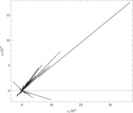
This is a clear indication for the existence of finite-time singularities in the cosmological system at hand. In Refs. Odintsov:2018uaw; Odintsov:2018awm, this issue was clearly explained, and following the discussions in Refs. Odintsov:2018uaw; Odintsov:2018awm, a dynamical system singularity, may be also a finite-time singularity for the cosmological system. In fact, a singularity in the variables , and may correspond to a Type III singularity or a Big Rip singularity of the cosmological system, we refer to Refs. Odintsov:2018uaw; Odintsov:2018awm for further details on this, and to Ref. Nojiri:2005sx for the classification of finite-time singularities.
In principle, it is very hard to find finite-time singularities using the dynamical systems approach, so one can rely on numerical investigations. We need to note though the finite-time singularities can be found by using some other analytic techniques beyond the dynamical system approach, see for example Barrow:2006xb; Ivanov:2011np. In addition, in Refs. Odintsov:2018uaw; Odintsov:2018awm we used a powerful technique, which we called “Dominant Balance Analysis”, which can be applied to any polynomial autonomous dynamical system. Since the dynamical system (13) is a polynomial dynamical system, we shall also make use of the dominant balance analysis in this paper too. The dominant balance analysis is based on a theorem proved in Ref. goriely, and this analysis was also used in cosmological contexts in Ref. barrowcotsakis. It is worth recalling its basic features in this paper too, which can be summarized in the following:
What we seek is proof that the variables of the dynamical system (13), namely, , and become infinite at some finite-time instance . So consider the general dynamical system,
| (29) |
with being a vector of , namely, , and a vector of of the form , where the functions are strictly polynomials of the variables of the dynamical system. At a finite-time singularity a variable of the dynamical system will be have as , with , so the method of goriely goes as follows,
- •
Find all possible truncations of the function in Eq. (29). A dominant truncation controls the evolution of the dynamical system near finite-time singularities, which we denote as , hence the dynamical system becomes,
(30) Many different truncations may be found, but finding a consistent truncation that satisfies the constraints we present now, is the main aim of the method. For a truncation , we write the dynamical system variables in the following form,
(31) so by assuming that the solution can be written in -series form as functions of , we substitute the ’s from Eq. (31) in Eq. (30). After that, one needs to equate the exponents of the resulting polynomials, and therefore the parameters , , are determined, which must be real fractional numbers or integers. We form the vector , and by equating the polynomials in Eqs. (30), (31), we obtain the coefficients , from which we form the vector . The set is called dominant balance.
- •
If takes complex values for some of the coefficients ’s, it is certain that the dynamical system develops no finite-time singularities. On the other hand if takes real non-zero values for all ’s, then the dynamical system develops finite-time singularities.
- •
The singular and non-singular solutions found in the previous step might correspond to general initial conditions or to a limited set of initial conditions, and this must be ensured. This feature can be validated by finding the Kovalevskaya matrix , which is defined as follows,
(32) which must be calculated at a non-zero balance of the previous step. Next one needs to calculate the eigenvalues of , which must have the form .
- •
If , , then the solutions, singular or not, are general solutions, which means that these correspond to a general set of initial conditions. In the opposite case, the solutions are not general and these correspond to a limited set of initial conditions.
In the case at hand, we will apply the method we presented above, having in mind that the variables and are required to satisfy the Friedmann constraint (11), even a singular point. The dynamical system (13) is written as , where is , and in addition the vector function is,
| (33) |
with the functions , being equal to,
| (34) | ||||
A consistent truncation of (33), is the following,
| (35) |
and by following the steps of the dominant balance analysis method, we easily obtain,
| (36) |
and also,
| (37) |
Clearly cannot be complex for any values of , hence we definitely have singular solutions. It now remains to determine whether the singular solutions are general or these correspond to a limited set of initial conditions. To this end, we evaluate the Kovalevskaya matrix , which is,
| (38) |
and when it is evaluated on , it is equal to,
| (39) |
the eigenvalues of which are,
| (40) |
Due to the fact that it contains negative eigenvalues, this indicates that the singular solutions found for the classical dark energy superfluid dark matter system are not general, which means that these correspond to a limited set of initial conditions.
In conclusion, our analysis of the phase space of the classical dark energy superfluid dark matter cosmological system indicates that no de Sitter fixed points exist, and the rest of the fixed points, which can be of various physical forms, for example radiation or matter domination ones, are strongly unstable. Also the dominant balance analysis we performed showed that there exist singular solutions which are not general solutions though, which means that these correspond to a limited set of initial conditions. What now remains is to investigate whether the LQC effects affect the phase space structure of the dark energy-dark matter system. This is the subject of the next section.
III The Loop Quantum Cosmology Framework and Interacting Dark Energy with Superfluid Dark Matter
Having discussed the classical phase space of the coupled dark energy superfluid dark matter system, in this section we shall thoroughly investigate the LQC phase space of this cosmological system. We shall focus on the existence of stable attractors, with particular emphasis given on de Sitter attractors, which are relevant for the late-time acceleration. Also we shall investigate whether the singular solutions of the classical dynamical system persist in the LQC case too. However it is worth discussing briefly what superfluid dark matter brings along and why it is worth studying. Superfluid dark matter was introduced in Ref. Berezhiani:2015bqa, and further developed in Refs. Berezhiani:2015pia; Hodson:2016rck; Berezhiani:2017tth. The dark matter superfluid model of Ref. Berezhiani:2015bqa has the appealing property of reproducing the -Cold Dark Matter model at large scales, and it simultaneously matches the phenomenological predictions of Modified Newtonian Dynamics on Galactic scales. In the theory of Ref. Berezhiani:2015bqa consists of axion-like particles with eV-scale mass, which strongly interact between them. The effects of the superfluid dark matter condensates are apparent only on galactic scales, but not when galactic clusters are considered. The resulting theory has many appealing observational features, like for example it explains the low-density vortices in galaxies, it also explains the infall dependent and phonon speed of sound low-density vortices in galaxies. In addition, bullet-like clusters are also very well fitted by the theory which leads to distinct mass peaks, and furthermore the the superfluid effective theory has similarities with a unitary Fermi Gas. For further discussions and phenomenological implications on superfluid dark matter, we refer the reader to Refs. Berezhiani:2015pia; Hodson:2016rck; Berezhiani:2017tth.
Before we start, we shall briefly review some essential information of LQC, and for details, the reader is referred to Refs. LQC1; LQC3; LQC4; LQC5; Salo:2016dsr; Xiong:2007cn; Amoros:2014tha; Cai:2014zga; deHaro:2014kxa; Kleidis:2018plu; Kleidis:2017ftt. We focus on holonomy corrected LQC, in the context of which, the spacetime is discrete, and the Hamiltonian of the theory is written in terms of the holonomies , where denote the Pauli matrices, and it is equal to,
| (41) |
In the Hamiltonian (41), the parameter is and it is the Barbero-Immirzi parameter, and also the parameter is , and it has dimension of length. Furthermore, stands for the spacetime volume, which for the flat FRW metric reads , and finally denotes the Universe’s total energy density. Moreover, the dynamical variable is the canonical conjugate variable , and these two have the following Poisson bracket . The trace of the Hamiltonian can easily be evaluated and it reads,
| (42) |
and by also taking into account the Hamiltonian constraint , we have,
| (43) |
which is the LQC version of the Friedmann equation. By taking into account the equation , then by combining the above we obtain,
| (44) |
which can be written as,
| (45) |
By using Eqs. (45) and (43), we obtain,
| (46) |
and after some algebraic manipulations, we obtain the final form of the LQC Friedmann equation, which has the following form,
| (47) |
The critical density parameter is of great importance, due to the fact that it is the maximum energy density of the LQC Universe, and it is equal to . Notably, the limit in Eq. (47) restores the classical Friedmann equation (3).
Let us now proceed in finding the LQC dynamical system of the coupled dark energy superfluid dark matter fluid for the flat FRW metric (1), so let us write the LQC Friedman equation in the following form,
| (48) |
with being in this case too the total energy density . The continuity equations for the dark energy and the dark matter fluids remain the same as in Eq. (5) and also the interaction term is assumed to have the form (6). Upon differentiation of Eq. (48) with respect to the cosmic time, in conjunction with Eq. (5), we get,
| (49) |
where is the total pressure which is equal to . In addition, for the purposes of this section, we assume that the dark energy EoS of equation (9), has the following form,
| (50) |
where is a free parameter of the theory, and also that the dark matter EoS has the superfluid form of the form,
| (51) |
where and are dimensionless constant parameters. Our aim is to construct a polynomial autonomous dynamical system for the cosmological system at hand, analogous to the one appearing in Eq. (13), so we shall choose the dimensionless variables of the dynamical system to have the following form in this case,
| (52) |
In view of Eq. (48), the variables , and satisfy the LQC version of the Friedmann constraint, which is,
| (53) |
Moreover, the total EoS parameter has in the LQC case the following form,
| (54) |
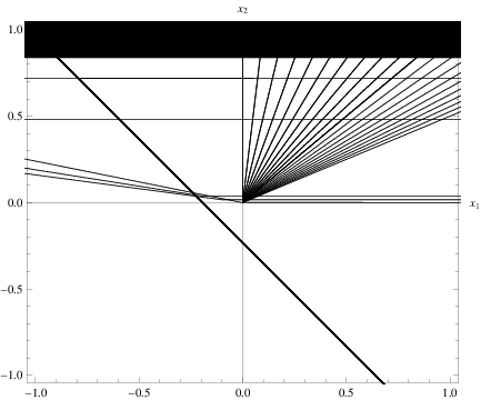
By combining Eqs. (48), (49), (5), and (52), and also by using the -foldings number as a dynamical variable, after some extensive algebraic manipulations, we obtain the dynamical system,
| (55) | ||||
where we also took into account Eq. (12). The dynamical system (55) describes the LQC coupled dark energy superfluid dark matter cosmological system, and it is an autonomous polynomial dynamical system, which we now study thoroughly. As we will demonstrate, the phase space structure of the LQC cosmological system is very rich. We start off with the fixed points, which are,
| (56) | ||||
where stands for,
| (57) |
Apart from the above, it can be shown that there exist other classes of fixed points, which are determined by the simultaneous validity of various algebraic equations, which are too lengthy to quote here. We denote these fixed points . Actually the class of fixed points are more interesting phenomenologically, since some of these are stable when the de Sitter cosmology is considered. In principle, by requiring or , we can obtain the radiation and matter domination fixed points, however we shall not be interested in these fixed points, but we emphasize on de Sitter fixed points, which as we show these exist. Let us start with the fixed point which is unphysical since the total EoS parameter is infinite, so let us proceed in the study of the fixed point . In this case we require that , which describes a de Sitter evolution. The condition is satisfied when,
| (58) |
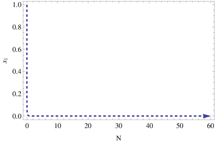
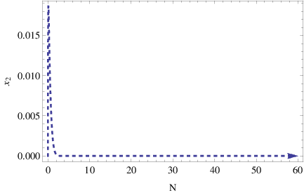
and this covers the fixed point too. So let us investigate the stability of these de Sitter vacua, and by calculating the Jacobian matrix and the corresponding eigenvalues, the resulting picture is that these vacua are hyperbolic fixed points, however unstable for all the values of and . Note that due to the extended and complicated form of the Jacobian matrix and of the resulting eigenvalues, we do not quote these here. Let us now investigate the stability of the class of fixed points , so we perform a numerical analysis for this case. The resulting picture is that for and for , , and for small negative values of , some de Sitter vacua of are hyperbolic fixed points with negative real parts of the eigenvalues of the Jacobian matrix, hence stability is ensured. In order to have a more clear picture of how the trajectories behave in the phase space, we shall perform a numerical investigation. As we shall see, the trajectories in the phase space approach a stable fixed point, and this can be seen in the numerical analysis of the phase space trajectories which we present in Fig. 2. As it can be seen in Fig. 2 where we plot the trajectories in the plane, and as it can be seen a stable equilibrium is reached by the trajectories for various initial conditions. Also, in Fig. 3 we plot the behavior of , and as functions of , for the values of the free parameters chosen as and , , , and as it can be seen a stable fixed point is reached.
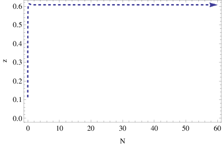
An important feature in order for stable and physically acceptable fixed points to occur, is that must be negative and also . If or if some of these are negative, the final value of the variable is negative, so this is not physically acceptable.
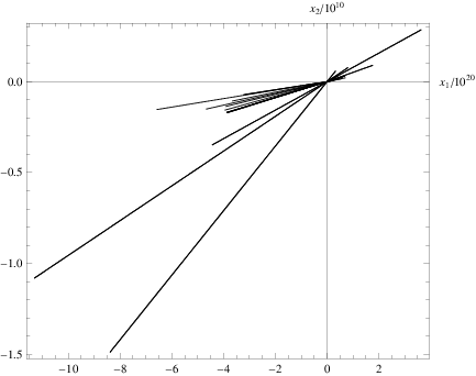
A deeper analysis revealed strong singular solutions, for which the variables blow-up, see for example Fig. 4, where we plot the trajectories in the plane. This mean that there exist initial conditions which make the variables blow-up strongly, and thus we shall use the dominant balance analysis we presented briefly in the previous section, in order to investigate whether the singular solutions correspond to general initial conditions or to a limited set of initial conditions.
To this end, we can write the dynamical system as (55) , with the vector being of the form , and in addition the vector function being defined in the following way,
| (59) |
with the functions , being equal to,
| (60) | ||||
A consistent truncation of the function appearing in Eq. (59), is the following,
| (61) |
The vector can easily be found by applying the method of the previous section, so we obtain,
| (62) |
and accordingly, the vector reads,
| (63) |
The vector can be complex for and real for , so we shall investigate both cases of the sign of the parameter . The Kovalevskaya matrix for the truncation (61) reads,
| (64) |
and therefore, when it is evaluated on it reads,
| (65) |
The eigenvalues of the above matrix are,
| (66) |
regardless of the choice of the parameter . Therefore, the resulting picture is quite interesting, since it validates our earlier numerical analysis considerations which indicated that for positive values of , singular solutions exist. Indeed, the eigenvalues (66) indicate that for positive , is real and therefore there exist singular solutions which correspond to general initial conditions (due to the form of the eigenvalues (66)), a feature that we also demonstrated in Fig. 4. Also, for negative , our analysis shows that no general singular solutions exist, but in this case, no stable de Sitter equilibria exist in the phase space of the LQC system. With regard to the relation of the dynamical system singular solutions (for ) with the finite time singularities, when and actually blow up, the finite-time singularities may be of Big Rip or even Type II or Type III type depending on the value of the parameter . Due to the form of the vector , we may conclude that in the case , both and blow up in the phase space, and therefore is finite, which means that the singularities are of Type III, according to the classification of Ref. Nojiri:2005sx. Finally, we need to question the physical significance of the cases with , since in this case, the dark matter EoS (8) would describe a negative pressure fluid, which is highly unlikely however. Hence the case is rather physically unappealing.
In conclusion, the LQC extended coupled dark energy superfluid dark matter cosmological system has interesting phase features, which we list in Table 1, along with the classical cosmological system and we discuss here in brief. The LQC system has many de Sitter vacua, which for can be stable de Sitter equilibria. Also for , general singular solutions exist in the phase space, along with stable de Sitter equilibria, which means that apart from the set of initial conditions which may lead to the stable de Sitter fixed points, there exist general initial conditions which lead to singular solutions. For however, we demonstrated that no singular solutions exist in the phase space. This behavior is to be contrasted with the classical case, where no de Sitter fixed points existed and also only a limited set of initial conditions leaded to singular solutions.
| Theoretical Framework | Existence and Stability of de Sitter Fixed points | Singular Solutions |
|---|---|---|
| Classical Case: | No de Sitter fixed Points | Non general singular solutions |
| LQC case: | Stable de Sitter fixed points for | General singular solutions for |
| LQC case: | Non-stable de Sitter fixed points for | No singular solutions for |
Before closing, an important question arises, related to the era were LQC effects are expected to be found. Particularly it is known that the LQC effects should be found in early-time eras, were gravity is expected to be considerably strong. In the case at hand, when interacting dark energy-dark matter fluids are considered in the context of LQC, we found stable de Sitter attractors for the theory. These attractor solutions should be interpreted correctly, mathematically these solutions exist, but the question is what do they represent? Obviously, this question cannot be answered by using only the fixed points of the dynamical system, since there is no obvious answer on when these fixed points are reached from the dynamical system. Our numerical analysis showed that these fixed points are reached quite fast, before the first sixty e-foldings, see for example Fig. 3. Thus these could be viewed as possibly some early-time inflationary attractors, which are reached quite fast from the dynamical system. Also the existence of singular solutions in this case, shows that there exist initial conditions in the system that will generate finite-time singularities, which possibly can be related to the late-time era, since the early-time era is quite stable and de Sitter like. To our opinion, in order to be accurate, the quantum equations of motion will be those of LQC only when the energy density of the Universe is quite close to , otherwise one effectively has the classical equations of motion. Therefore, the possible interpretation of the results is that the dark energy fluid coupled with the dark matter fluid gives some early inflationary attractors in the theory, when LQC are strong, but as the Universe evolves, and the cosmological equations become effectively classical, the coupled superfluid dark matter-dark energy system has no de Sitter attractor solutions. Thus this makes superfluid dark matter quite important for early-time considerations, at least when dark energy is represented by a fluid coupled to the dark matter fluid. We need to note that it is quite interesting to check whether the superfluid composed by axion-like particles has strong effects if it is considered in the context of other theories, like for example modified gravity. Work is in progress in this research line.
IV Conclusions
In this paper we investigated the classical and the LQC phase space of a cosmological system consisting of two interacting dark fluids, namely the dark energy fluid and the superfluid dark matter fluid. For the dark matter fluid we assumed that the EoS describes superfluid dark matter, so the fluid has non-zero pressure, in contrast to cold dark matter which is pressureless. With regard to the classical case, we investigated the existence and stability of cosmological fixed points, and as we demonstrated there exist matter and radiation domination fixed points which are unstable, however no de Sitter fixed points occur in the phase space for any value of the free parameters. Due to the structure of the dynamical system, which was a polynomial autonomous dynamical system, we were able to perform a dominant balance analysis, which revealed that no general singular solutions exist, however singular solutions corresponding to a limited set of initial conditions exist. With regard to the LQC phase space, the situation is much more interesting due to the fact that the phase space contains much more physical structures in comparison to the classical one. Specifically, in this case stable de Sitter fixed points occur when the free parameter , appearing in the superfluid dark matter EoS, is positive. In this case too, the phase space has also singular solutions, which correspond to a general set of initial conditions, so these are general solutions. In addition, the singular solutions of the dynamical system correspond to Type III physical finite-time singularities. We believe that we covered the most general case for the coupled system of dark energy and superfluid dark matter system, and the only modification which could be done in principle is to use an EoS for the dark energy fluid of the form , , which could have strong effects in the singularity occurrence phenomenon. We defer this task to a future work. Different EoS for dark energy, such as logarithmic Odintsov:2018obx or even Chaplygin gas, like in the form used in Bamba:2012cp; Bento:2002ps; Bilic:2001cg (see also Khurshudyan:2018kfk where a non-trivial interacting varying Chaplygin gas EoS is used with tachyonic matter, which would correspond to in the case studied in this paper), would make the form of the dynamical system quite complicated, since it would cease to be a polynomial dynamical system, so the method of dominant balance analysis which we used in this paper, would be inapplicable in this case. Such a task would require different approaches, and work is in progress along this research line.
References
- (1) A. G. Riess et al. [Supernova Search Team], Astron. J. 116 (1998) 1009 doi:10.1086/300499 [astro-ph/9805201].
- (2) V. K. Oikonomou, J. D. Vergados and C. C. Moustakidis, Nucl. Phys. B 773 (2007) 19 doi:10.1016/j.nuclphysb.2007.03.014 [hep-ph/0612293].
- (3) S. Nojiri, S. D. Odintsov and V. K. Oikonomou, Phys. Rept. 692 (2017) 1 doi:10.1016/j.physrep.2017.06.001 [arXiv:1705.11098 [gr-qc]].
- (4) S. Nojiri, S.D. Odintsov, Phys. Rept. 505, 59 (2011);
- (5) S. Nojiri, S.D. Odintsov, eConf C0602061, 06 (2006) [Int. J. Geom. Meth. Mod. Phys. 4, 115 (2007)].
- (6)
S. Capozziello, M. De Laurentis,
Phys. Rept. 509, 167 (2011);
V. Faraoni and S. Capozziello, Fundam. Theor. Phys. 170 (2010). doi:10.1007/978-94-007-0165-6 - (7) A. de la Cruz-Dombriz and D. Saez-Gomez, Entropy 14 (2012) 1717 doi:10.3390/e14091717 [arXiv:1207.2663 [gr-qc]].
- (8) G. J. Olmo, Int. J. Mod. Phys. D 20 (2011) 413 doi:10.1142/S0218271811018925 [arXiv:1101.3864 [gr-qc]].
- (9) S. Nojiri and S. D. Odintsov, Phys. Rev. D 68 (2003) 123512 doi:10.1103/PhysRevD.68.123512 [hep-th/0307288].
- (10) P. Gondolo and K. Freese, Phys. Rev. D 68 (2003) 063509 doi:10.1103/PhysRevD.68.063509 [hep-ph/0209322].
- (11) G. R. Farrar and P. J. E. Peebles, Astrophys. J. 604 (2004) 1 doi:10.1086/381728 [astro-ph/0307316].
- (12) R. G. Cai and A. Wang, JCAP 0503 (2005) 002 doi:10.1088/1475-7516/2005/03/002 [hep-th/0411025].
- (13) Z. K. Guo, R. G. Cai and Y. Z. Zhang, JCAP 0505 (2005) 002 doi:10.1088/1475-7516/2005/05/002 [astro-ph/0412624].
- (14) B. Wang, J. Zang, C. Y. Lin, E. Abdalla and S. Micheletti, Nucl. Phys. B 778 (2007) 69 doi:10.1016/j.nuclphysb.2007.04.037 [astro-ph/0607126].
- (15) O. Bertolami, F. Gil Pedro and M. Le Delliou, Phys. Lett. B 654 (2007) 165 doi:10.1016/j.physletb.2007.08.046 [astro-ph/0703462 [ASTRO-PH]].
- (16) J. H. He and B. Wang, JCAP 0806 (2008) 010 doi:10.1088/1475-7516/2008/06/010 [arXiv:0801.4233 [astro-ph]].
- (17) J. Valiviita, E. Majerotto and R. Maartens, JCAP 0807 (2008) 020 doi:10.1088/1475-7516/2008/07/020 [arXiv:0804.0232 [astro-ph]].
- (18) B. M. Jackson, A. Taylor and A. Berera, Phys. Rev. D 79 (2009) 043526 doi:10.1103/PhysRevD.79.043526 [arXiv:0901.3272 [astro-ph.CO]].
- (19) M. Jamil, E. N. Saridakis and M. R. Setare, Phys. Rev. D 81 (2010) 023007 doi:10.1103/PhysRevD.81.023007 [arXiv:0910.0822 [hep-th]].
- (20) J. H. He, B. Wang and E. Abdalla, Phys. Rev. D 83 (2011) 063515 doi:10.1103/PhysRevD.83.063515 [arXiv:1012.3904 [astro-ph.CO]].
- (21) Y. L. Bolotin, A. Kostenko, O. A. Lemets and D. A. Yerokhin, Int. J. Mod. Phys. D 24 (2014) no.03, 1530007 doi:10.1142/S0218271815300074 [arXiv:1310.0085 [astro-ph.CO]].
- (22) A. A. Costa, X. D. Xu, B. Wang, E. G. M. Ferreira and E. Abdalla, Phys. Rev. D 89 (2014) no.10, 103531 doi:10.1103/PhysRevD.89.103531 [arXiv:1311.7380 [astro-ph.CO]].
- (23) C. G. Boehmer, G. Caldera-Cabral, R. Lazkoz and R. Maartens, Phys. Rev. D 78 (2008) 023505 doi:10.1103/PhysRevD.78.023505 [arXiv:0801.1565 [gr-qc]].
- (24) S. Li and Y. Ma, Eur. Phys. J. C 68 (2010) 227 doi:10.1140/epjc/s10052-010-1338-y [arXiv:1004.4350 [astro-ph.CO]].
- (25) W. Yang, S. Pan and J. D. Barrow, arXiv:1706.04953 [astro-ph.CO].
- (26) S. D. Odintsov, V. K. Oikonomou, A. V. Timoshkin, E. N. Saridakis and R. Myrzakulov, Annals Phys. 398 (2018) 238 doi:10.1016/j.aop.2018.09.015 [arXiv:1810.01276 [gr-qc]].
- (27) K. Bamba, S. Capozziello, S. Nojiri and S. D. Odintsov, Astrophys. Space Sci. 342 (2012) 155 doi:10.1007/s10509-012-1181-8 [arXiv:1205.3421 [gr-qc]].
- (28) J. D. Barrow and J. P. Mimoso, Phys. Rev. D 50 (1994) 3746. doi:10.1103/PhysRevD.50.3746
- (29) C. G. Tsagas and J. D. Barrow, Class. Quant. Grav. 15 (1998) 3523 doi:10.1088/0264-9381/15/11/016 [gr-qc/9803032].
- (30) W. S. Hipolito-Ricaldi, H. E. S. Velten and W. Zimdahl, JCAP 0906 (2009) 016 doi:10.1088/1475-7516/2009/06/016 [arXiv:0902.4710 [astro-ph.CO]].
- (31) V. Gorini, A. Kamenshchik, U. Moschella, V. Pasquier and A. Starobinsky, Phys. Rev. D 72 (2005) 103518 doi:10.1103/PhysRevD.72.103518 [astro-ph/0504576].
- (32) G. M. Kremer, Phys. Rev. D 68 (2003) 123507 doi:10.1103/PhysRevD.68.123507 [gr-qc/0309111].
- (33) I. Brevik, V. V. Obukhov and A. V. Timoshkin, Int. J. Geom. Meth. Mod. Phys. 15 (2018) no.09, 1850150 doi:10.1142/S0219887818501505 [arXiv:1805.01258 [gr-qc]].
- (34) D. Carturan and F. Finelli, Phys. Rev. D 68 (2003) 103501 doi:10.1103/PhysRevD.68.103501 [astro-ph/0211626].
- (35) T. Buchert, Gen. Rel. Grav. 33 (2001) 1381 doi:10.1023/A:1012061725841 [gr-qc/0102049].
- (36) J. c. Hwang and H. Noh, Class. Quant. Grav. 19 (2002) 527 doi:10.1088/0264-9381/19/3/308 [astro-ph/0103244].
- (37) N. Cruz, S. Lepe and F. Pena, Phys. Lett. B 699 (2011) 135. doi:10.1016/j.physletb.2011.03.049
- (38) V. K. Oikonomou, Int. J. Mod. Phys. D 26 (2017) no.10, 1750110 doi:10.1142/S0218271817501103 [arXiv:1703.09009 [gr-qc]].
- (39) I. Brevik, E. Elizalde, S. D. Odintsov and A. V. Timoshkin, Int. J. Geom. Meth. Mod. Phys. 14 (2017) no.12, 1750185 doi:10.1142/S0219887817501857 [arXiv:1708.06244 [gr-qc]].
- (40) I. Brevik, O. Gron, J. de Haro, S. D. Odintsov and E. N. Saridakis, Int. J. Mod. Phys. D 26 (2017) no.14, 1730024 doi:10.1142/S0218271817300245 [arXiv:1706.02543 [gr-qc]].
- (41) S. Nojiri and S. D. Odintsov, Phys. Rev. D 72 (2005) 023003 doi:10.1103/PhysRevD.72.023003 [hep-th/0505215].
- (42) S. Capozziello, S. Nojiri, S. D. Odintsov and A. Troisi, Phys. Lett. B 639 (2006) 135 doi:10.1016/j.physletb.2006.06.034 [astro-ph/0604431].
- (43) S. Nojiri and S. D. Odintsov, Phys. Lett. B 639 (2006) 144 doi:10.1016/j.physletb.2006.06.065 [hep-th/0606025].
- (44) E. Elizalde and D. Saez-Gomez, Phys. Rev. D 80 (2009) 044030 doi:10.1103/PhysRevD.80.044030 [arXiv:0903.2732 [hep-th]].
- (45) E. Elizalde and M. Khurshudyan, arXiv:1711.01143 [gr-qc].
- (46) I. Brevik and A. V. Timoshkin, Int. J. Geom. Meth. Mod. Phys. 14 (2017) no.04, 1750061 doi:10.1142/S021988781750061X [arXiv:1612.06689 [gr-qc]].
- (47) A. B. Balakin and V. V. Bochkarev, Phys. Rev. D 87 (2013) no.2, 024006 doi:10.1103/PhysRevD.87.024006 [arXiv:1212.4094 [gr-qc]].
- (48) W. Zimdahl and A. B. Balakin, Class. Quant. Grav. 15 (1998) 3259 doi:10.1088/0264-9381/15/10/026 [gr-qc/9807078].
- (49) S. D. Odintsov, V. K. Oikonomou, A. V. Timoshkin, E. N. Saridakis and R. Myrzakulov, arXiv:1810.01276 [gr-qc].
- (50) M. Kunz, Phys. Rev. D 80 (2009) 123001 doi:10.1103/PhysRevD.80.123001 [astro-ph/0702615].
- (51) L. Berezhiani and J. Khoury, Phys. Rev. D 92 (2015) 103510 doi:10.1103/PhysRevD.92.103510 [arXiv:1507.01019 [astro-ph.CO]].
- (52) L. Berezhiani and J. Khoury, Phys. Lett. B 753 (2016) 639 doi:10.1016/j.physletb.2015.12.054 [arXiv:1506.07877 [astro-ph.CO]].
- (53) A. Hodson, H. Zhao, J. Khoury and B. Famaey, Astron. Astrophys. 607 (2017) A108 doi:10.1051/0004-6361/201630069 [arXiv:1611.05876 [astro-ph.CO]].
- (54) L. Berezhiani, B. Famaey and J. Khoury, arXiv:1711.05748 [astro-ph.CO].
- (55) S. Tulin and H. B. Yu, Phys. Rept. 730 (2018) 1 doi:10.1016/j.physrep.2017.11.004 [arXiv:1705.02358 [hep-ph]].
- (56) S. D. Odintsov and V. K. Oikonomou, Phys. Rev. D 98 (2018) no.2, 024013 doi:10.1103/PhysRevD.98.024013 [arXiv:1806.07295 [gr-qc]].
- (57) S. D. Odintsov and V. K. Oikonomou, Phys. Rev. D 97 (2018) no.12, 124042 doi:10.1103/PhysRevD.97.124042 [arXiv:1806.01588 [gr-qc]].
- (58) S. D. Odintsov and V. K. Oikonomou, arXiv:1902.01422 [gr-qc].
- (59) C. G. Boehmer and N. Chan, doi:10.1142/9781786341044.0004 arXiv:1409.5585 [gr-qc].
- (60) C. G. Boehmer, T. Harko and S. V. Sabau, Adv. Theor. Math. Phys. 16 (2012) no.4, 1145 doi:10.4310/ATMP.2012.v16.n4.a2 [arXiv:1010.5464 [math-ph]].
- (61) N. Goheer, J. A. Leach and P. K. S. Dunsby, Class. Quant. Grav. 24 (2007) 5689 doi:10.1088/0264-9381/24/22/026 [arXiv:0710.0814 [gr-qc]].
- (62) G. Leon and E. N. Saridakis, JCAP 1504 (2015) no.04, 031 doi:10.1088/1475-7516/2015/04/031 [arXiv:1501.00488 [gr-qc]].
- (63) J. Q. Guo and A. V. Frolov, Phys. Rev. D 88 (2013) no.12, 124036 doi:10.1103/PhysRevD.88.124036 [arXiv:1305.7290 [astro-ph.CO]].
- (64) G. Leon and E. N. Saridakis, Class. Quant. Grav. 28 (2011) 065008 doi:10.1088/0264-9381/28/6/065008 [arXiv:1007.3956 [gr-qc]].
- (65) J. C. C. de Souza and V. Faraoni, Class. Quant. Grav. 24 (2007) 3637 doi:10.1088/0264-9381/24/14/006 [arXiv:0706.1223 [gr-qc]].
- (66) A. Giacomini, S. Jamal, G. Leon, A. Paliathanasis and J. Saavedra, Phys. Rev. D 95 (2017) no.12, 124060 doi:10.1103/PhysRevD.95.124060 [arXiv:1703.05860 [gr-qc]].
- (67) G. Kofinas, G. Leon and E. N. Saridakis, Class. Quant. Grav. 31 (2014) 175011 doi:10.1088/0264-9381/31/17/175011 [arXiv:1404.7100 [gr-qc]].
- (68) G. Leon and E. N. Saridakis, JCAP 1303 (2013) 025 doi:10.1088/1475-7516/2013/03/025 [arXiv:1211.3088 [astro-ph.CO]].
- (69) T. Gonzalez, G. Leon and I. Quiros, Class. Quant. Grav. 23 (2006) 3165 doi:10.1088/0264-9381/23/9/025 [astro-ph/0702227].
- (70) A. Alho, S. Carloni and C. Uggla, JCAP 1608 (2016) no.08, 064 doi:10.1088/1475-7516/2016/08/064 [arXiv:1607.05715 [gr-qc]].
- (71) S. K. Biswas and S. Chakraborty, Int. J. Mod. Phys. D 24 (2015) no.07, 1550046 doi:10.1142/S0218271815500467 [arXiv:1504.02431 [gr-qc]].
- (72) D. Muller, V. C. de Andrade, C. Maia, M. J. Reboucas and A. F. F. Teixeira, Eur. Phys. J. C 75 (2015) no.1, 13 doi:10.1140/epjc/s10052-014-3227-2 [arXiv:1405.0768 [astro-ph.CO]].
- (73) B. Mirza and F. Oboudiat, Int. J. Geom. Meth. Mod. Phys. 13 (2016) no.09, 1650108 doi:10.1142/S0219887816501085 [arXiv:1412.6640 [gr-qc]].
- (74) S. Rippl, H. van Elst, R. K. Tavakol and D. Taylor, Gen. Rel. Grav. 28 (1996) 193 doi:10.1007/BF02105423 [gr-qc/9511010].
- (75) M. M. Ivanov and A. V. Toporensky, Grav. Cosmol. 18 (2012) 43 doi:10.1134/S0202289312010100 [arXiv:1106.5179 [gr-qc]].
- (76) M. Khurshudyan, Int. J. Geom. Meth. Mod. Phys. 14 (2016) no.03, 1750041. doi:10.1142/S0219887817500414
- (77) R. D. Boko, M. J. S. Houndjo and J. Tossa, Int. J. Mod. Phys. D 25 (2016) no.10, 1650098 doi:10.1142/S021827181650098X [arXiv:1605.03404 [gr-qc]].
- (78) S. D. Odintsov, V. K. Oikonomou and P. V. Tretyakov, Phys. Rev. D 96 (2017) no.4, 044022 doi:10.1103/PhysRevD.96.044022 [arXiv:1707.08661 [gr-qc]].
- (79) L. N. Granda and D. F. Jimenez, arXiv:1710.07273 [gr-qc].
- (80) F. F. Bernardi and R. G. Landim, Eur. Phys. J. C 77 (2017) no.5, 290 doi:10.1140/epjc/s10052-017-4858-x [arXiv:1607.03506 [gr-qc]].
- (81) R. C. G. Landim, Eur. Phys. J. C 76 (2016) no.1, 31 doi:10.1140/epjc/s10052-016-3894-2 [arXiv:1507.00902 [gr-qc]].
- (82) R. C. G. Landim, Eur. Phys. J. C 76 (2016) no.9, 480 doi:10.1140/epjc/s10052-016-4328-x [arXiv:1605.03550 [hep-th]].
- (83) P. Bari, K. Bhattacharya and S. Chakraborty, arXiv:1805.06673 [gr-qc].
- (84) S. Chakraborty, arXiv:1805.03237 [gr-qc].
- (85) M. G. Ganiou, P. H. Logbo, M. J. S. Houndjo and J. Tossa, arXiv:1805.00332 [gr-qc].
- (86) P. Shah, G. C. Samanta and S. Capozziello, arXiv:1803.09247 [gr-qc].
- (87) V. K. Oikonomou, Int. J. Mod. Phys. D 27 (2018) no.05, 1850059 doi:10.1142/S0218271818500591 [arXiv:1711.03389 [gr-qc]].
- (88) S. D. Odintsov and V. K. Oikonomou, Phys. Rev. D 96 (2017) no.10, 104049 doi:10.1103/PhysRevD.96.104049 [arXiv:1711.02230 [gr-qc]].
- (89) J. Dutta, W. Khyllep, E. N. Saridakis, N. Tamanini and S. Vagnozzi, JCAP 1802 (2018) 041 doi:10.1088/1475-7516/2018/02/041 [arXiv:1711.07290 [gr-qc]].
- (90) S. D. Odintsov and V. K. Oikonomou, Phys. Rev. D 93 (2016) no.2, 023517 doi:10.1103/PhysRevD.93.023517 [arXiv:1511.04559 [gr-qc]].
- (91) K. Kleidis and V. K. Oikonomou, arXiv:1808.04674 [gr-qc].
- (92) A. Ashtekar and P. Singh, Class. Quant. Grav. 28 (2011) 213001 [arXiv:1108.0893 [gr-qc]]
- (93) A. Ashtekar, T. Pawlowski and P. Singh, Phys. Rev. Lett. 96 (2006) 141301 [gr-qc/0602086].
- (94) A. Ashtekar, T. Pawlowski and P. Singh, Phys. Rev. D 73 (2006) 124038 [gr-qc/0604013].
- (95) A. Ashtekar, T. Pawlowski and P. Singh, Phys. Rev. D 74 (2006) 084003 [gr-qc/0607039].
- (96) L. Areste Salo, J. Amoros and J. de Haro, Class. Quant. Grav. 34 (2017) no.23, 235001 doi:10.1088/1361-6382/aa9311 [arXiv:1612.05480 [gr-qc]].
- (97) H. H. Xiong, T. Qiu, Y. F. Cai and X. Zhang, Mod. Phys. Lett. A 24 (2009) 1237 doi:10.1142/S0217732309030667 [arXiv:0711.4469 [hep-th]].
- (98) J. Amoros, J. de Haro and S. D. Odintsov, Phys. Rev. D 89 (2014) no.10, 104010 doi:10.1103/PhysRevD.89.104010 [arXiv:1402.3071 [gr-qc]].
- (99) Y. F. Cai and E. Wilson-Ewing, JCAP 1403 (2014) 026 doi:10.1088/1475-7516/2014/03/026 [arXiv:1402.3009 [gr-qc]].
- (100) J. de Haro and J. Amoros, JCAP 1408 (2014) 025 doi:10.1088/1475-7516/2014/08/025 [arXiv:1403.6396 [gr-qc]].
- (101) K. Kleidis and V. K. Oikonomou, Int. J. Geom. Meth. Mod. Phys. 15 (2018) no.05, 1850071 doi:10.1142/S0219887818500718 [arXiv:1801.02578 [gr-qc]].
- (102) K. Kleidis and V. K. Oikonomou, Int. J. Geom. Meth. Mod. Phys. 15 (2017) no.04, 1850064 doi:10.1142/S0219887818500640 [arXiv:1711.09270 [gr-qc]].
- (103) M. Sami, P. Singh and S. Tsujikawa, Phys. Rev. D 74 (2006) 043514 doi:10.1103/PhysRevD.74.043514 [gr-qc/0605113].
- (104) S. Nojiri, S. D. Odintsov and S. Tsujikawa, Phys. Rev. D 71 (2005) 063004 doi:10.1103/PhysRevD.71.063004 [hep-th/0501025].
- (105) G. Caldera-Cabral, R. Maartens and L. A. Urena-Lopez, Phys. Rev. D 79 (2009) 063518 doi:10.1103/PhysRevD.79.063518 [arXiv:0812.1827 [gr-qc]].
- (106) D. Pavon and W. Zimdahl, Phys. Lett. B 628 (2005) 206 doi:10.1016/j.physletb.2005.08.134 [gr-qc/0505020].
- (107) M. Quartin, M. O. Calvao, S. E. Joras, R. R. R. Reis and I. Waga, JCAP 0805 (2008) 007 doi:10.1088/1475-7516/2008/05/007 [arXiv:0802.0546 [astro-ph]].
- (108) H. M. Sadjadi and M. Alimohammadi, Phys. Rev. D 74 (2006) 103007 doi:10.1103/PhysRevD.74.103007 [gr-qc/0610080].
- (109) W. Zimdahl, Int. J. Mod. Phys. D 14 (2005) 2319 doi:10.1142/S0218271805007784 [gr-qc/0505056].
- (110) J. D. Barrow and S. Hervik, Phys. Rev. D 74 (2006) 124017 doi:10.1103/PhysRevD.74.124017 [gr-qc/0610013].
- (111) M. Ivanov and A. V. Toporensky, Int. J. Mod. Phys. D 21 (2012) 1250051 doi:10.1142/S0218271812500514 [arXiv:1112.4194 [gr-qc]].
- (112)
A. Goriely, C Hyde, Journal of Differential Equations 161, 422-448 (2000)
https://doi.org/10.1006/jdeq.1999.3688 - (113) S. Cotsakis and J. D. Barrow, J. Phys. Conf. Ser. 68 (2007) 012004 doi:10.1088/1742-6596/68/1/012004 [gr-qc/0608137].
- (114) M. C. Bento, O. Bertolami and A. A. Sen, Phys. Rev. D 66 (2002) 043507 doi:10.1103/PhysRevD.66.043507 [gr-qc/0202064].
- (115) N. Bilic, G. B. Tupper and R. D. Viollier, Phys. Lett. B 535 (2002) 17 doi:10.1016/S0370-2693(02)01716-1 [astro-ph/0111325].
- (116) M. Khurshudyan, Int. J. Geom. Meth. Mod. Phys. 15 (2018) no.09, 1850155. doi:10.1142/S0219887818501554