In this paper we focus on $2\to 2$ S-matrix elements of identical particles of mass $m$, with incoming momenta $p_{1},p_{2}$ and outgoing momenta $-p_{4},-p_{3}$, ordered according to figure 1. The Mandelstam variables are defined as

In terms of the relative rapidity $\theta$ of particles 1 and 2, we can write

Note that the map from $s$ to $\theta$ is not single-valued, and the choice of branch will be determined through the analytic continuation procedure (see figure 2).

The $2\to 2$ S-matrix element, denoted simply $S(s)$, is an analytic function on the complex $s$-plane (“first sheet”) away from the branch cuts along $(-\infty,0]\cup[4m^{2},\infty)$, the $s$-channel pole at $s=m^{2}$ and the $t$-channel pole at $s=3m^{2}$, as well as other possible poles corresponding to on-shell particles in the $s$ or $t$ channel.

We will further assume that the particle of mass $m$ is the lightest particle in the theory. Under this assumption there will be no further singularities on the $s$-plane corresponding to anomalous thresholds [13, 14]. Resonances, on the other hand, correspond to poles on the “second sheet” of $S(s)$ analytically continued through the branch cut of $2$ particle states of the lightest particle.

Crossing symmetry amounts to

The physical $2\to 2$ scattering amplitude is given by the value of $S(s)$ approaching the right branch cut from above, namely

For physical energies in the $s$-channel, $S(s)$ is subject to the unitarity constraint

In particular, below the inelastic threshold, namely for $4m^{2}\leq s\leq{\rm min}((m+m_{2})^{2},9m^{2})$, where $m_{2}$ is the mass of the second lightest particle (if it exists), we have $|S(s)|=1$.

Furthermore, $S(s)$ is subject to the real analyticity condition

where $S(s^{*})$ is defined as the value of $S(s^{\prime})$ at $s^{\prime}=s^{*}$ on the first sheet. It follows that the value of $S(s)$ approaching the branch cut $[4m^{2},\infty)$ from below is the complex conjugate of the physical amplitude.

On the complex rapidity $\theta$-plane, the branch cuts are located at $\theta\in(-\infty,-\theta_{0}]\cup[\theta_{0},\infty)$ along the real $\theta$ axis and their translations by integer multiples of $\pi i$, where $\theta_{0}$ is the rapidity value that corresponds to the inelastic threshold. The pole at $s=m^{2}$ and $3m^{2}$ translate to poles at $\theta={2\pi i\over 3}$ and ${\pi i\over 3}$, as well as their images under shifts by integer multiples of $2\pi i$. Physical amplitudes are given by

The first sheet of the complex $s$-plane is mapped to the “physical strip” $0<{\rm Im}\,\theta<\pi$. The second sheet corresponds to $-\pi<{\rm Im}\,\theta<0$. The crossing symmetry is expressed in terms of $S(\theta)$ as

The real analyticity condition can be expressed as

This is because the regions above and below the physical cut $s\in[4m^{2},\infty)$ on the $s$-plane, related by complex conjugation, are mapped to the regions above the positive and negative real $\theta$ axis on the $\theta$-plane, which are related by complex conjugation combined with a sign flip (see figure 2).

The unitarity constraint can be expressed as

where $f(\theta)$ is a real-valued function for $\theta\in\mathbb{R}$ that obeys $f(\theta)=1$ for $|\theta|<\theta_{0}$ and $f(\theta)\leq 1$ for $|\theta|\geq\theta_{0}$. Since $S(\theta)S^{*}(\theta)=1$ in the elastic regime, we can analytically continue this relation to the whole physical strip, and write

It follows that poles in the physical strip (first sheet) correspond to zeros on the second sheet and vice versa (see figure 2).

It is generally expected from causality [13, 15] that all poles on the $\theta$-plane away from the above mentioned branch cuts are either due to intermediate on-shell particles (poles on the physical strip) or resonances (poles on the second sheet). It is further expected that in a local quantum field theory $S(s)$ is bounded near infinity on the $s$-plane [16, 17, 18].³³ 3 The usual statement is that $S(s)$ is polynomial bounded at large complex $s$. Together with the unitarity bound along the physical branch cut, a theorem of Fuchs [19] implies that $S(s)$ is in fact bounded at large complex $s$. Under these assumptions, we can write $S(\theta)$ in the form

where $f(\theta)$ is the function appearing in (2.10). $S_{\rm CDD}(\theta)$, known as the Castillejo-Dalitz-Dyson (CDD) factor, is meromorphic on the physical strip and is a pure phase for real $\theta$.

If one further assumes that there is no essential singularity at infinity, then the CDD factor can be written as

The ${\alpha}_{j}$’s with ${\rm Re}({\alpha}_{j})\in(0,\pi)$ give rise to poles in the physical strip, which we refer to as “CDD poles”, whereas those with ${\rm Re}({\alpha}_{j})\in(-\pi,0)$ give rise to poles on the second sheet, or zeros in the physical strip, which we refer to as “CDD resonances” or “CDD zeros”. The CDD poles are due to intermediate on-shell particles, and are expected to lie on the imaginary $\theta$-axis (absent anomalous thresholds). The CDD zeros could be anywhere in the physical strip, and would generally come in quadruples with respect to the reflection $\theta\to-\theta^{*}$ and with respect to crossing transformation $\theta\to\pi i-\theta$, unless either ${\rm Re}\,\theta=0$ or ${\rm Im}\,\theta={\pi\over 2}$.

In the rest of this paper, while we will be guided by (2.13) in producing the numerical approximation of $S(\theta)$, the method of bounding the error in section 2.2 does not require the assumption of absence of essential singularity at infinity.

To proceed, it will be convenient to introduce the $z$ variable

(2.14) maps half of the physical strip, namely the domain $0\leq{\rm Im}\,\theta\leq{\pi\over 2}$, to the unit disc $|z|\leq 1$. The physical amplitude is given by the value of $S(z)$ at the boundary of the unit $z$-disc. We will denote by ${\cal I}$ the arc on the boundary of the disc that correspond to the image of $[-\theta_{0},\theta_{0}]$, where $S(z)$ is a phase, and by ${\cal J}$ the complement of ${\cal I}$ on the boundary of the disc that correspond to energies above the inelastic threshold where $|S(z)|\leq 1$ (see figure 3).

The $t$-channel pole at $\theta={\pi i\over 3}$, due to the exchange of a particle that is identical to the external particles, is mapped to $z=0$. Any other poles of $S(z)$ on the unit $z$-disc would correspond to the exchange of another (stable) particle, whose mass is between $m$ and $2m$ (since we have assumed that the external particle of mass $m$ is the lightest). Such a pole corresponds to a CDD factor of the form

where $z_{*}$ lies on the interval $(-1,7-4\sqrt{3})$ (corresponding to purely imaginary values of $\theta$).

Resonances, on the other hand, correspond to zeros of $S(z)$ in the unit disc. They come in complex conjugate pairs due to the relation $S(z)=(S(z^{*}))^{*}$, unless they lie on the real $z$-axis.

The function

where the product over $j$ ranges over all CDD poles other than the one at $z=0$, is analytic in the interior of the unit $z$ disc, obeys $|g(z)|\leq 1$ on the boundary of the disc, and by assumption is bounded near $z=1$ in the interior of the disc. Note that we will not need to assume the absence of essential singularity at $z=1$, allowing for instance the possibility of gravitational dressing factors in the S-matrix [20, 18].

Our objective is to determine $g(z)$ from its values on the arc ${\cal I}$, namely the elastic scattering phases that will be computed independently in the next section using TFFSA and Luscher’s method. For this, we make use of the following

The proof of the above lemma is given in Appendix A.

For our application, $F(z)$ will be the difference between the function $g(z)$ defined in (2.16) and a trial function $\widetilde{g}(z)$ with similar properties (e.g. $|\widetilde{g}(z)|\leq 1$ on the unit circle) that closely approximates $g(z)$ in the elastic regime (the arc ${\cal I}$). The lemma then places a bound on the “error” $|g(z)-\widetilde{g}(z)|$ in the interior of the disc. In this case, $B_{z}\leq 2$, and we will simply replace $B_{z}$ by 2 in practical evaluations of the error bound. We now describe two practical methods of constructing such numerical approximations of $g(z)$.

In terms of the $z$ variable, we can write (2.12) as

where $\mathfrak{f}(\phi)$ is $f(\theta)$ evaluated at $z=e^{i\phi}$. $-\log\mathfrak{f}(\phi)$ is expected to be a positive even function in the range $\phi\in(-\phi_{0},\phi_{0})$, corresponding to energies above the particle production threshold.

Our approximation to $g(z)$ takes the form

where $Q(x)$ is taken to be a sum of squares of polynomials, constrained by $Q(1)=0$. The “trial zeros” $z_{1}^{\prime},\cdots,z_{M}^{\prime}$ as well as $Q(x)$ are chosen by fitting the phase of $\widetilde{g}(z)$ to that of $g(z)$ on the elastic arc ${\cal I}$.

Application of both methods will be illustrated in section 4. We find method II more feasible in practice, as in many cases the scattering phase can be reliably extracted from TFFSA only on a set of disjoint arcs in the elastic regime. Nonetheless, the error bound given by the lemma is typically quite small away from the inelastic arc ${\cal J}$, when reasonable assumptions on resonance zeros are made. A priori, zeros of $S(z)$ can appear anywhere on the $z$-disc, so long as they come in complex conjugate pair when they are away from the real line. In IFT, as we increase $\eta$ from zero to positive values, the 5 heavier particles of $E_{8}$ theory are expected to turn into complex resonances. The simplest possibility is that the only other zeros of $S(z)$ appear on the real interval $(-1,1)$. Our analysis will be consistent with this scenario in that, by numerically fitting (2.25) with $z_{k}^{\prime}$ constrained to lie on the real interval $(-1,1)$, we will be able to rigorously bound the error of our approximation to $S(z)$ on the $z$-disc, and exclude the possibility of additional complex zeros outside of a small neighborhood of the inelastic arc ${\cal J}$.

Let us comment that the existence of analytic continuation to the interior of the $z$-disc subject to the unitarity bounds on the boundary and the analytic assumptions imposes highly nontrivial constraints on the elastic scattering data themselves. Numerical errors in the elastic data (as obtained from TFFSA) could in principle lead to different fits of $S(z)$ with incompatible (e.g. mutually exclusive) error bounds.

Note that the error bound becomes loose near the inelastic arc on the boundary of the $z$-disc. Indeed, based on effective field theory one expects that the low energy scattering data is insensitive to a high energy resonance of very small width.

To compute the energy spectrum of Ising field theory on a cylinder of radius $R$, we write the Hamiltonian as

where $H_{0}$ is the Hamiltonian of a free Majorana fermion field of mass $|m_{f}|$ that results from the Ising CFT deformed by the energy operator. The free fermion Hilbert space ${\cal H}^{\rm free}$ and the spectrum of $H_{0}$, however, depend on the sign of the deformation parameter $m_{f}$. ${\cal H}^{\rm free}$ is the direct sum of Neveu-Schwarz (NS) and Ramond (R) sectors,

where ${\cal H}_{\rm NS}$ is spanned by states of the form

where $N$ is an even positive integer, and $n_{i}$ are distinct momentum quantum numbers (in units of $1/R$) of the $N$ fermions. The R sector, on the other hand, is spanned by states of the form

where $N$ is odd for the “high temperature” theory with $m_{f}>0$, and even for the “low temperature” theory with $m_{f}<0$. A fermion mode labeled by $n$ carries momentum $p_{n}$ and energy $\omega_{n}$,

The ground state energy of NS and R sector are denoted $E_{0}^{\rm NS}(R)$ and $E_{0}^{\rm R}(R)$ respectively, with their difference given by

where we write $E\equiv\sqrt{p^{2}+m_{f}^{2}}$. Note that in the large $R$ limit, (3.6) is of order $e^{-|m_{f}|R}$.

The spin field $\sigma$ has only nonzero matrix elements (form factors) between NS and R sector states, given by [7]⁵⁵ 5 In [7] $R$ denotes the circumferences of the circle, whereas here we use $R$ to denote the radius, hence a factor $2\pi$ difference.

where

with $A_{G}$ being Glaisher’s constant and the functions $s(R)$ and $\kappa(R,p)$ are given by

where we again wrote $E\equiv\sqrt{p^{2}+m_{f}^{2}}$ and similarly for $E^{\prime}$. Note that both $s(R)$ and $\kappa(R,p)$ vanish in the $R\to\infty$ limit.

We will restrict to the sector of the Hilbert space with zero total momentum along the circle. Starting from the free massive fermion Hilbert space, including both NS and R sectors, we will truncate to the finite dimensional subspace spanned by states involving any number of left or right moving fermions, such that the total right moving momentum is no more than $L/R$. $L$ will be referred to as the “truncation level”. We then evaluate the matrix elements of the IFT Hamiltonian for a basis of the truncated Hilbert space, and numerically diagonalize the resulting finite dimensional Hamiltonian matrix to obtain the energy spectrum. This is known as the TFFSA [6]. The error of such an approximation to the energy levels is expected to be suppressed by inverse powers of the truncation level $L$, as a consequence of asymptotic decoupling between low and high energy states [21, 22].

A typical set of resulting energy spectrum obtained from TFFSA is shown in figure 4. In this example we have taken the truncation level $L=19$, fixing a suitable choice of the circle radius $R$ in units of $|h|^{-{8\over 15}}$, and scanned over a range of $\eta$. In the plot we displayed the first 10 energy levels after subtracting the ground state energy, and normalized in units of the first excitation energy (identified with the mass $m_{1}$ of the lightest particle). The energy levels below $2m_{1}$ correspond to stable particles, whereas those above $2m_{1}$ generically correspond to scattering states.

To minimize the error due to level truncation, we can perform an extrapolation to $L=\infty$ by fitting the finite level data to

following [7]. In determining the mass of the stable particles, we first extrapolate the excitation energies to $L=\infty$ at fixed radii $R$, and then extrapolate to infinite radius using an exponential fit.

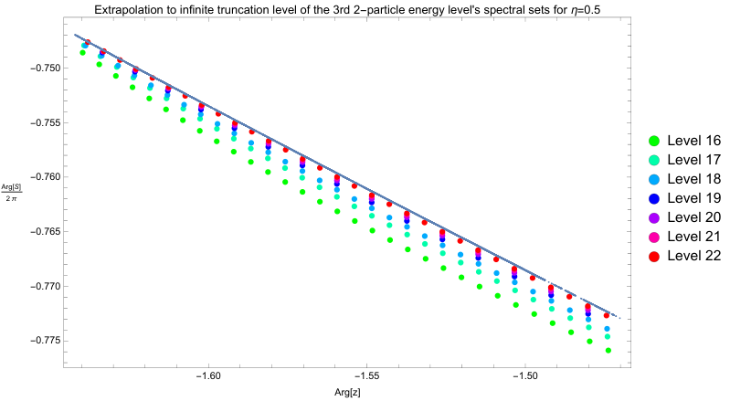
As for the scattering states in the elastic regime, we work at a given truncation level $L$ and extract the scattering phase using Luscher’s method as explained in the next section, for a range of radii. We then extrapolate the resulting graph for the scattering phase as a function of energy to $L=\infty$ by a power law fit analogous to (3.11).

Focusing on the energy range of elastic scattering states of two of the lightest particle with zero total momentum, we define the spectral set

Here the energies $E_{n}$ are labeled by the level $n$ in increasing order, with the understanding that for sufficiently large radius $R$, $E_{n}$ can be thought of as the scattering state of a pair of particles carrying momentum $p_{n}$ and $-p_{n}$ on the circle, with

such that $p_{n}$ is subject to the Bohr-Sommerfeld quantization condition

where $\varphi(E)$ is the elastic scattering phase at center of mass energy $E$. Thus, for sufficiently large $R$, the spectral set ${\cal S}$ is expected to lie on the graph of the function ${1\over 2\pi}\varphi(E)$. Examples of finite size effects are shown in Figure 5. On the other hand, errors due to the level truncation in TFFSA becomes worse at large $R$. The convergence with increasing truncation level is demonstrated in Figure 6.

In practice, it is typically sufficient to take the union of spectral sets collected over suitable moderate ranges of $R$. The smallness of finite size effects is justified a posteriori by observing the approximate overlap of spectral sets for different energy levels of 2-particle states, as demonstrated in Figure 7.

We now present results on the $2\to 2$ scattering amplitude $S(z)$ of the lightest particle in IFT, analytically continued into the interior of the complex $z$-disc (or equivalently, to the physical strip in the $\theta$-plane). We adopt method II of section 2.2, in which we begin by making simple assumptions on the number of CDD/resonance zeros of $S(z)$ on the disc, and then fit both the CDD zero locations and the function $\mathfrak{f}(\phi)$ in (2.24) against the elastic scattering phase computed using TFFSA via Luscher’s method.

Our data for the elastic phase is subject to two types of errors: those due to level truncation on the Hamiltonian in TFFSA, and finite size effects on the circle of radius $R$. The former is handled by an extrapolation to infinite truncation level using (3.11). The finite size effects, which corrects both the mass of the particles and the quantization condition (3.14), is exponentially suppressed at sufficiently large $R$. As the TFFSA data are collected over a range of $R$, the finite size effects are handled by imposing a suitable lower bound on $R$, as illustrated in section 3.2. Consequently, the reliable data for the elastic phase may only cover a collection of disjoint arcs ${\cal I}^{\prime}$ within the elastic arc ${\cal I}$ on the boundary of the $z$-disc. In this case, we simply replace ${\cal I}$ by ${\cal I}^{\prime}$ in applying the method of section 2.2.

To assume a certain number of resonance zeros may appear to be a gross (and incorrect) simplification. However, the Lemma of section 2.2 gives a rigorous bound on the error of such a fit to $S(z)$ in the interior of the disc, provided that its errors on elastic arc ${\cal I}$, or rather the subset ${\cal I}^{\prime}$, are known. That is to say, if we could ignore the error in determining the elastic scattering phase and the stable particle masses from TFFSA, we would have a rigorous bound on the analytically continued $S(z)$ despite the presumption on the resonance zeros. If the error bound in the interior of the $z$-disc ends up small, then our assumptions are justified a posteriori. On the other hand, if we made incorrect assumptions on the locations of resonance zeros, the error bounds would necessarily be large in the relevant domain, thereby indicating that the fit for $S(z)$ is problematic.

From the residues of $S(z)$ at its poles, we can extract the on-shell 3-point coupling $g_{j}$ between two lightest particles and the $j$-th lightest particle via [18]

where $z_{j}$ is the pole position corresponding to the mass $m_{j}$ of the exchanged particle in either $s$ or $t$-channel. The error bound on our numerical approximation to $S(z)$ in the disc allows us to bound the error of the residue. The results for $g_{111}$ and $g_{112}$ at positive $\eta$ are shown in Figure 9 (note that the second stable particle only exists up to a finite value of $\eta$).

As $\eta$ increases past certain positive values, the second lightest particle (of mass $m_{2}$) and the third lightest particle (of mass $m_{3}$) turn into resonances, as will be discussed in section 4.2. These resonances will appear as simple zeros of $S(z)$ on the real axis at $z_{2}^{\prime}$ and $z_{3}^{\prime}$ respectively. The numerical determination of $z_{2}^{\prime}$ and $z_{3}^{\prime}$, together with error bars obtained from (2.17), are shown in Figures 10. Note that the graphs for $z_{2}^{\prime}$ and $z_{3}^{\prime}$ as functions of $\eta$ smoothly join those of $1/z_{2}$ and $1/z_{3}$ ($z_{j}$ being the pole associated with the $j$-th stable particle), as expected from the poles moving into the second sheet.

The fourth lightest particle (of mass $m_{4}$), on the other hand, gives rise to a pair of resonance zeros $z_{4}^{\prime}$ and $z_{4}^{\prime*}$ at complex values near the boundary of the $z$-disc. Our numerical results for $z_{4}^{\prime}$ over a range of $\eta$ is shown in the LHS of Figure 15.

While there may well be other resonance zeros that are not taken into account by our approximation to $S(z)$, the error bound (2.17) allow us to exclude their presence in much of the $z$-disc. Such exclusion plots are shown in Figure 11, where unknown resonances are excluded in the yellow region but are possible in the blue “non-exclusion” regions. For a view of the analogous exclusion plot on the $s$-plane, see Figure 12. Note that our error bound is loose near $z=-1$ and near $z=1$, giving rise to non-exclusion regions near both. The non-exclusion region near $z=-1$ is presumably an artifact of our approach, as Luscher’s method does not allow us to access the elastic scattering at energies very close to $2m_{1}$. It is very unlikely that there would be unknown low energy resonances near $z=-1$. On the other hand, there may well be unknown resonances in the non-exclusion region near $z=1$ (high energy limit).

For $0.2<\eta\leq 1.6$, it turns out that including an additional pair of complex zeros $z_{x}^{\prime}$ and $(z_{x}^{\prime})^{*}$, corresponding to a narrow resonance with energy above the inelastic threshold, improves the fit for $S(z)$ and reduces the error bounds. While our fit suggests the existence of such a resonance, the latter cannot be justified rigorously through our error bound. In particular, the non-exclusion region where we cannot rule out the existence of extra resonance zeros has a connected domain that contains both $z_{x}^{\prime}$ and the inelastic arc ${\cal J}$, as shown in the RHS of Figure 15. In contrast, the other known resonances (including $z_{4}^{\prime}$) lie in their own “islands” of non-exclusion regions (these islands are too small to be visible in Fig 11). A comparison of the error bounds for $zS(z)$ at real $z$ with or without including $z_{x}^{\prime}$ in the fit is shown in Figure 21.

Finally, our numerical results for $\log|S(z)|$ on the entire unit disc and $zS(z)$ on the real interval $(-1,1)$ are shown in Figure 13 and Figure 14 respectively, with the error bounds indicated in the latter.

We now describe a simple scenario for the evolution of the poles and zeros of $S(z)$ as functions of $\eta$, which was proposed in [1] and is corroborated by our results. We focus on positive real values of $\eta$, interpolating between the $E_{8}$ affine Toda theory at $\eta=0$ and the free fermion point in the high temperature limit $\eta\to+\infty$.

Starting at $\eta=0$, where the IFT is integable (Figure 13a), $S(z)$ is known to be given exactly by the CDD factors associated with three poles. Apart from the self-coupling pole at $z=0$, there is a CDD pole at $z_{2}\approx 0.0467965$ corresponding to the second lightest particle with $m_{2}=2\cos{\pi\over 5}m_{1}$, and another CDD pole at $z_{3}\approx-0.612751$ corresponding to the third lightest particle with $m_{3}=2\cos{\pi\over 30}m_{1}$. There is no particle production and no resonance in this case. The infinite energy limit of the S-matrix element is $S(z=1)=1$.

A pole of $S(z)$ can only leave the disc by meeting a mirror zero on the second sheet at $z=-1$ (see Figures 13, 14), as the corresponding particle becomes unstable. Note that $S(z=-1)=-1$ is maintained throughout. When a pole leaves the first sheet, its mirror zero enters the disc as a resonance zero. In particular, the third lightest particle (of mass $m_{3}$) decays at $\eta\approx 0.144$, where the pole $z_{3}$ moves out of the disc and the zero $z_{3}^{\prime}$ enters. As $\eta$ increases, $z_{3}^{\prime}$ moves along the real $z$-axis with increasing $\eta$ (Figures 13b-13e) toward $z=1$.

We do not know the fate of $z_{3}^{\prime}$ at large $\eta$. There are three possible scenarios. One possibility is that $z_{3}^{\prime}$ reaches $z=1$ at a finite value of $\eta$ (around $\approx 1.8$ by our crude estimate) and then disappears from the disc. Another possibility is that $z_{3}^{\prime}$ “stays” at $z=1$ rather than “exits” the disc, and that $S(z)$ vanishes at $z=1$ for $\eta$ greater than some finite value (the latter is suggested by [23]). The third possibility is that $z_{3}^{\prime}$ meets another zero of $S(z)$ on the real $z$-axis, and become a pair of complex resonances which then move toward the inelastic arc on the boundary, as $\eta$ increases. This scenario is quite plausible as it is similar to the expected behavior of complex resonances at negative $\eta$ (discussed at the end of this section).

The second lightest particle (of mass $m_{2}$) becomes unstable at $\eta\approx 2.078$, where the pole $z_{2}$ moves out of the disc and the zero $z_{2}^{\prime}$ enters from $z=-1$. As $\eta$ increases further, $z_{2}^{\prime}$ moves to the right along the real $z$ axis (Figures 13f-13h), and approaches $z=0$ as $\eta\to\infty$. In the latter limit, $z_{2}^{\prime}$ annihilates the self-coupling pole at $z=0$, as the lightest particle becomes a free fermion.

Simultaneously, as $\eta$ becomes nonzero, the 5 heavier particles of the $E_{8}$ theory immediately decay and give rise to complex resonances [1, 24]. In particular, the mass $m_{4}$ of the fourth lightest particle is below the inelastic threshold at $\eta=0$. For a range of positive $\eta$, the corresponding resonance zero $z_{4}^{\prime}$ (and its complex conjugate $z_{4}^{\prime*}$) is close to the boundary of the $z$-disc, and is visible as a jump by $2\pi$ in the elastic scattering phase (see Figure 8 for $\eta=0.3$ and $0.8$). We can take into account such a pair of CDD zeros in the ansatz for fitting $S(z)$ (via method II of section 2.2), which then allows us to determine the position of $z_{4}^{\prime}$ up to a small known bound on its error.

The evolution of $z_{4}^{\prime}$ with $\eta$ between 0 and $1.6$ is portrayed in the LHS of Figure 15. It begins at the point corresponding to $m_{4}=4\cos{\pi\over 5}\cos{7\pi\over 30}$, and stays close to the elastic arc for $\eta$ up to $\approx 2$. Note that the inelastic threshold $m_{1}+m_{2}$ moves with $\eta$ until $m_{2}$ reaches $2m_{1}$ and the second lightest particle decays. In Figure 16, we show the real and imaginary part of the energy of the $z_{4}^{\prime}$ resonance for positive $\eta$, with a comparison to results from leading order form factor perturbation theory around $\eta=0$ [10, 11].⁶⁶ 6 We thank G. Mussardo and G. Takács for bringing the results of [10, 11] to our attention.

For $\eta\leq 1.8$, we find reasonably good fitting for $S(z)$ with the additional complex resonance zero $z_{x}^{\prime}$ included, but with large uncertainty in the location of $z_{x}^{\prime}$ (RHS of Figure 15). We are unable to determine reliably the location or the existence of $z_{x}^{\prime}$ or any higher energy resonances, e.g. those coming from the more massive particles at the $\eta=0$ point, corresponding to pairs of complex zeros, or other possible real zeros near $z=1$.

As for the “low temperature” $\eta<0$ regime, where more stable particles (“mesons”) are present in the spectrum of IFT, some preliminary results on the elastic scattering phase are presented in Figure 17. Here we see evidence for the way in which the fourth stable particle enters the spectrum, suggested in [2]. Namely, as $\eta$ is decreased below 0, the $m_{4}$ resonance becomes wider and moves to lower energies, until its corresponding pair of complex zeros in the $z$-disc meet on the real $z$-axis. As $\eta$ is decreased further, one of the zeros moves in the positive-$z$ direction, remaining a resonance, whereas the other zero moves toward $z=-1$. The latter eventually exits the disc, as its mirror pole enters at $z=-1$ from the second sheet, giving rise to the stable $m_{4}$ particle. The $m_{5}$ resonance is visible in Figure 17 as well. Detailed corroboration and further analysis of the low temperature regime are of interest and are left for future work.

In the elastic scattering regime, that is, for $|\theta|<\theta_{0}$ where $\theta_{0}$ is the rapidity at the inelastic threshold, the deviation of the scattering phase from that of the CDD factor is related to the function $f(\theta)$ in (2.12) via

Note that in this regime (4.2) is positive and monotonically increasing. $f(\theta)$ is further related to the total inelastic scattering probability $\sigma_{\rm tot}(\theta)$ via

For weak magnetic field $h$ in the high temperature regime, namely $\eta\gg 1$, there is only one stable particle, and $\sigma_{\rm tot}(\theta)$ is dominated by the $2\to 3$ scattering probability $\sigma_{2\to 3}(\theta)$. The latter is computed to order $h^{2}$ in [23], with the result (written in $m_{f}=1$ units)

where $A_{G}$ is Glaisher’s constant, $E\equiv 2\cosh{\theta\over 2}$, and $\mu,\nu,\lambda$ are defined as

The leading perturbative contribution to $\Delta\phi(\theta)$ is

A comparison between our numerical fit for the (non-perturbative) S-matrix element $S(z)$ and the perturbative result based on (4.4), (4.6) is shown in Figure 18. The agreement is close for $\eta=2.4$ and nearly perfect for $\eta=4$.

In applying method II to determine the analytic continuation of $S(z)$ from the elastic arc ${\cal I}$ to the interior of the $z$-disc, we have fitted the function $f(\theta)$ appearing in (2.12) or (2.24). Naively, this could give a numerical estimate of the inelastic scattering probability via (4.3). However, the bound (2.17) becomes loose when $z$ approaches the inelastic arc ${\cal J}$ on the boundary of the disc, and we cannot rigorously bound the error on the fit for $f(\theta)$. Our inability to exclude narrow resonances close to the inelastic arc $\mathcal{J}$ is the other side of the same coin, as their effects on the elastic phase can hardly be distinguished numerically from (4.2) due to inelastic processes.⁷⁷ 7 For instance, had we missed a CDD zero $z_{*}^{\prime}$ (and its complex conjugate) close to the inelastic arc ${\cal J}$, with $z_{*}^{\prime}={\sinh(\theta_{*}+i\delta_{*})-{\sqrt{3}\over 2}i\over\sinh(\theta_{*}+i\delta_{*})+{\sqrt{3}\over 2}i}$ for real $\theta_{*}>\theta_{0}$ and small positive $\delta_{*}$, the corresponding CDD factor $\displaystyle{\sinh(\theta_{*}+i\delta_{*})-\sinh\theta\over\sinh(\theta_{*}+i\delta_{*})+\sinh\theta}\cdot{\sinh(-\theta_{*}+i\delta_{*})-\sinh\theta\over\sinh(-\theta_{*}+i\delta_{*})+\sinh\theta}=e^{-2i\delta_{*}\left[{1\over\sinh(\theta-\theta_{*})}+{1\over\sinh(\theta+\theta_{*})}\right]+{\cal O}(\delta_{*}^{3})}$ (4.7) would imitate a contribution to $-\log f(\theta)$ by $4\pi\delta_{*}\delta(\theta-\theta_{*})+{\cal O}(\delta_{*}^{3})$, resulting in an extra “resonance peak” in the numerical fit for $-\log f(\theta)$.

References

- [1] A. Zamolodchikov, Ising Spectroscopy II: Particles and poles at , arXiv:1310.4821.
- [2] P. Fonseca and A. Zamolodchikov, Ising spectroscopy. I. Mesons at T ¡ T(c), hep-th/0612304.
- [3] A. B. Zamolodchikov, Integrals of Motion and S Matrix of the (Scaled) T=T(c) Ising Model with Magnetic Field, Int. J. Mod. Phys. A4 (1989) 4235.
- [4] T. J. Hollowood and P. Mansfield, Rational Conformal Field Theories At, and Away From, Criticality as Toda Field Theories, Phys. Lett. B226 (1989) 73.
- [5] H. W. Braden, E. Corrigan, P. E. Dorey, and R. Sasaki, Affine Toda Field Theory and Exact S Matrices, Nucl. Phys. B338 (1990) 689–746.
- [6] V. P. Yurov and A. B. Zamolodchikov, Truncated fermionic space approach to the critical 2-D Ising model with magnetic field, Int. J. Mod. Phys. A6 (1991) 4557–4578.
- [7] P. Fonseca and A. Zamolodchikov, Ising field theory in a magnetic field: Analytic properties of the free energy, hep-th/0112167.
- [8] M. Luscher, Volume Dependence of the Energy Spectrum in Massive Quantum Field Theories. 1. Stable Particle States, Commun. Math. Phys. 104 (1986) 177.
- [9] M. Luscher, Volume Dependence of the Energy Spectrum in Massive Quantum Field Theories. 2. Scattering States, Commun. Math. Phys. 105 (1986) 153–188.
- [10] G. Delfino, G. Mussardo, and P. Simonetti, Nonintegrable quantum field theories as perturbations of certain integrable models, Nucl. Phys. B473 (1996) 469–508, [hep-th/9603011].
- [11] B. Pozsgay and G. Takacs, Characterization of resonances using finite size effects, Nucl. Phys. B748 (2006) 485–523, [hep-th/0604022].
- [12] M. Luscher, Signatures of unstable particles in finite volume, Nucl. Phys. B364 (1991) 237–251.
- [13] R. J. Eden, P. V. Landshoff, D. I. Olive, and J. C. Polkinghorne, The analytic S-matrix. Cambridge Univ. Press, Cambridge, 1966.
- [14] P. Goddard, Anomalous threshold singularities in s-matrix theory, Nuovo Cim. A59 (1969) 335–355.
- [15] X. O. Camanho, J. D. Edelstein, J. Maldacena, and A. Zhiboedov, Causality Constraints on Corrections to the Graviton Three-Point Coupling, JHEP 02 (2016) 020, [arXiv:1407.5597].
- [16] A. M. Jaffe, HIGH-ENERGY BEHAVIOR OF LOCAL QUANTUM FIELDS, .
- [17] H. Epstein, V. Glaser, and A. Martin, Polynomial behaviour of scattering amplitudes at fixed momentum transfer in theories with local observables, Commun. Math. Phys. 13 (1969) 257–316.
- [18] M. F. Paulos, J. Penedones, J. Toledo, B. C. van Rees, and P. Vieira, The S-matrix bootstrap II: two dimensional amplitudes, JHEP 11 (2017) 143, [arXiv:1607.06110].
- [19] W. H. J. Fuchs, A phragmén-Lindelöf theorem conjectured by d. j. newman, Trans. Amer. Math. Soc. 267 (1981), no. 1 285–293.
- [20] S. Dubovsky, R. Flauger, and V. Gorbenko, Solving the Simplest Theory of Quantum Gravity, JHEP 09 (2012) 133, [arXiv:1205.6805].
- [21] P. Giokas and G. Watts, The renormalisation group for the truncated conformal space approach on the cylinder, arXiv:1106.2448.
- [22] M. Hogervorst, S. Rychkov, and B. C. van Rees, Truncated conformal space approach in d dimensions: A cheap alternative to lattice field theory?, Phys. Rev. D91 (2015) 025005, [arXiv:1409.1581].
- [23] A. Zamolodchikov and I. Ziyatdinov, Inelastic scattering and elastic amplitude in Ising field theory in a weak magnetic field at : Perturbative analysis, Nucl. Phys. B849 (2011) 654–674, [arXiv:1102.0767].
- [24] G. Delfino, P. Grinza, and G. Mussardo, Decay of particles above threshold in the Ising field theory with magnetic field, Nucl. Phys. B737 (2006) 291–303, [hep-th/0507133].
- [25] S. Rychkov and L. G. Vitale, Hamiltonian truncation study of the theory in two dimensions, Phys. Rev. D91 (2015) 085011, [arXiv:1412.3460].
- [26] S. Rychkov and L. G. Vitale, Hamiltonian truncation study of the theory in two dimensions. II. The -broken phase and the Chang duality, Phys. Rev. D93 (2016), no. 6 065014, [arXiv:1512.00493].