Shadowed FSO/mmWave Systems with Interference
Abstract
We investigate the performance of mixed free space optical (FSO)/millimeter-wave (mmWave) relay networks with interference at the destination. The FSO/mmWave channels are assumed to follow Málaga-/ Generalized- fading models with pointing errors in the FSO link. The H-transform theory, wherein integral transforms involve Fox’s H-functions as kernels, is embodied to unifying the performance analysis framework that encompasses closed-form expressions for the outage probability, the average bit error rate (BER) and the average capacity. By virtue of some H-transform asymptotic expansions, the high signal-to-interference-plus-noise ratio (SINR) analysis reduces to easy-to-compute expressions for the outage probability and BER, which reveals inside information for the system design. We finally investigate the optimal power allocation strategy, which minimizes the outage probability. ††footnotetext: Work supported by the Discovery Grants and the CREATE PERSWADE (www.create-perswade.ca) programs of NSERC and a Discovery Accelerator Supplement (DAS) Award from NSERC.
Index Terms:
Millimeter wave, dual-hop relaying, free-space optics (FSO), cochannel interference (CCI), Málaga- fading, power allocation, shadowing.I Introduction
Millimeter wave (mmWave) small-cell concept is envisioned to enable extremely high data rates and ubiquitous coverage through the resources reuse over smaller areas and the huge amount of available spectrum. One significant concern in the deployment of such networks is backhauling in order to handle the unprecedented data traffic surge between all small cells across the network. Recently, due to its cost-efficient and high data rate capabilities and immunity to interference, the current perspectives advocate the use of free-space optics (FSO) technology as a promising solution for constructing low-cost backhaul for small-cells. In this perspective, relay-assisted FSO-based backhaul framework and mmWave-based access links, where relays are applied as optical to radio frequency (RF) “converter” to assist the communications of small cells, is considered as a powerful candidate to provide high-data rate reliable communications in high-density heterogeneous networks [1], [2]. Nevertheless, several hurdles must be overcome to enable mixed FSO/mmWave communications and make them work properly. One of the major challenges facing the application of FSO communication is its vulnerability to atmospheric turbulence and strong path-loss [3]. On the RF side, on the other hand, the mmWave signals can be blocked due to shadowing thereby inferring coverage holes that prevent mmWave communication from delivering uniform capacity for all users in the network [4]. Moreover, in ultra-dense cellular networks, the mmWave RF interference issue may arise when the signals emitted from a large number of unintended transmitters are captured by the beam at an intended receiver via line-of-sight (LoS) and/or reflection paths, thereby critically exacerbating the link quality deterioration [5].
I-A State-of-The Art and Motivation
In recent years, understanding the fundamental performance limits of mixed FSO/RF systems has attracted a lot of research interest (see [6]-[16] and references therein). Also, the effective utilization of resources (e.g., power) in both combined systems becomes of paramount importance. In [6] and [7], the authors investigated the performance of an amplify-and-forward (AF) mixed RF/FSO relay network over Nakagami- and Gamma-Gamma fading channels. Exact closed-form and analytical expressions were, respectively, derived in [6] and [7] for the outage probability, average bit error rate (BER), and channel capacity. Considering the outdated channel-state-information (CSI) effect on the RF link and misalignment error on the FSO link, the authors in [8] evaluated the performance of an AF mixed RF/FSO relay network over Rayleigh and Gamma-Gamma fading models. The same system model was studied in [9], but with - and - fading models for the RF link and a Gamma-Gamma fading model for the FSO link. Whereas it was studied in [10] assuming Rayleigh fading for the RF link and a Málaga- distribution model for the FSO link. In [11], the authors investigated the performance of an AF mixed RF/FSO relay network while including the direct link between the source and destination. They assumed Nakagami- fading model for the RF links and a generalized Gamma-Gamma fading model for the FSO link when deriving closed-form expressions for the outage and bit error probabilities. Work on AF mixed RF/FSO relay networks continued in [12] where the authors considered a millimeter-wave (mmWave) Rician distributed RF channel and a Málaga- distributed FSO channel. The same system model was also considered in [13], while assuming Weibull and Gamma-Gamma fading models for the mmWave RF and FSO links, respectively. In [14], the authors studied the performance of a mixed FSO/RF relay network assuming Málaga-/shadowed - fading models. They derived exact and asymptotic (i.e., at high signal-to-noise ratio (SNR) values) closed-form expressions for the system outage probability and channel capacity. Several studies on the effect of interference on the performance of AF mixed FSO/RF relay networks are presented in [15], [16], and [17]. The mixed RF/FSO relay network was investigated in [18] from a security point of view and in a cognitive radio scenario in [19]. The performance of an AF mixed RF/FSO relay network with multiple antennas at the source and multiple apertures at the destination was investigated in [20]. Most recently, Balti et al. [21] proposed a mixed RF/FSO system with general model of hardware impairments considering optical channels with Gamma-Gamma fading.
Although the results from [6]-[16] are insightful, these works have been successfully tractable only for small-scale fading channels on the RF links or Málaga- FSO links. To the best of our knowledge, the performance analysis of mixed FSO/mmWave systems under Málaga- distribution and composite fading conditions where fading and shadowing phenomena occur simultaneously has not been investigated in the open literature. In fact, in mmWave networks, both the desired and interfering signals are adversely effected by shadowing from objects over the signal path due to high directivity or due to human body movements [22]. Shadowing along with the high attenuation are the main drawbacks at mmWave frequencies that hinder successful transmission. As such, a careful characterization of the mixed FSO/mmWave system over composite fading conditions is crucial to identify the negatives of higher attenuation and shadowing. However, since composite fading distributions are steadily challenging, a friendlier analytical approach that typically allows the derivation of tractable expressions for key performance measures and indicators of interest is in fact desirable, yet still missing. While the work in [14] provides innovative characterization of mixed FSO/RF relay systems in fading channels where only dominant LOS components are affected by Nakagami- distributed shadowing, co-channel interference has not been considered. In fact, the incorporation of RF mmWave interference has been, so far, steadily overlooked (e.g., see [12], [20]) in the mixed FSO/RF context.
In this paper, we tackle the above issues by providing holistic analytical tools facilitating the evaluation of the mixed FSO/mmWave relay network performance by considering general cases, i.e., shadowed small-scale fading both on the desired and interference links, which are more challenging to analyze than only including distance-dependent path loss or rayleigh fading [21]-[23].
I-B Technical Contribution
In this paper, we investigate the performance of a dual-hop mixed FSO/mmWave relay network. To model mmWave composite multi-path shadowing fading, we consider generalized- distribution ([24],[25], [26]) with parameters and where different values represent LOS and NLOS cases [23] and indicates the mmWave sensitivity to blockages. To mitigate the effects of multi-path fading, the relay-to-destination mmWave-based hop uses a multiple-input-single-output (MISO) setup with transmit antennas. We further assume that the FSO link undergoes Málaga- distribution. Furthermore, it is assumed that the destination is affected by independent identically distributed co-channel interference in the mmWave band. The contribution of this paper can be summarized as follows:
- •
Using the theory of Fox’s H-functions and Mellin–Barnes integrals, we propose a novel mathematical framework to derive closed-form expressions for important statistics of the SINR under the assumption of fixed and variable-gain relaying, while not making any assumptions in our derivations, in terms of the bivariate Fox’s H function.
- •
New analytical results for the outage probability, the average error probability, and average capacity are derived. Our analysis procedure and performance metrics formulations are given in unified and tractable mathematical fashion thereby serving as a useful tool to validate and compare the special cases of Málaga- and generalized- distributions.
- •
An asymptotic outage and error rate performance analysis is presented, which enables the characterization of the key performance indicators, such as the diversity gain and coding gain, size of transmit array, effect of pointing error and shadowing on the achieved performance under the presence of interference.
- •
Capitalizing on the achieved asymptotic results, the optimum relay power allocation that minimizes the system outage probability is derived.
I-C Organization
The remainder of this paper is organized as follows. We describe the system and channel models in Section II. In Section III, we present the unifying H-transform analysis of the end-to-end SINR statistics for both fixed-gain and channel-state-information (CSI)-assisted mixed FSO/mmWave networks. Then, in section IV, we derive exact closed-form expressions for the outage probability, the average error probability and the average capacity followed by their asymptotic expressions obtained at high SINR. In section V, the optimum design strategy for FSO/mmWave networks is studied. Section VI presents some numerical and simulation results to illustrate the mathematical formalism presented in the previous sections. Finally, some concluding remarks are drawn out in Section VII.
II System Model
We consider the downlink of a relay-assisted network featuring a mixed FSO/mmWave communication link as shown in Fig. 1. The source is assumed to include a single photo-aperture, while the relay node is assumed to have a single photo detector from one side and antennas from the other side. The relay is able to activate either heterodyne or intensity modulation/direct (IM/DD) detection. Using amplify-and-forward (AF) relaying, all the transmit antennas at the relay are used for MRT (maximum ratio transmission) to communicate with the destination over the mmWave band. In the first hop, the FSO signal undergoes a Málaga- turbulent-induced fading channel, while in the second hop, the mmWave signals undergoes a generalized- fading channel. We further assume that the destination is affected by interferers. The interferers affecting have independent identically distributed generalized- fading.

II-A Optical Channel Model
The FSO (-) channel follows a Málaga- distribution for which the cumulative density function (CDF) of the instantaneous SNR in the presence of pointing errors is given by [27, Eq. (5)]
| (1) | |||||
where is the ratio between the equivalent beam radius and the pointing error displacement standard deviation (i.e., jitter) at the relay (for negligible pointing errors ), and , where , , and are the fading parameters related to the atmospheric turbulence conditions [27], [28]. It may be useful to mention that where is the average power of the LOS term and represents the amount of scattering power coupled to the LOS component ()11 1 It is worth highlighting that the distribution unifies most of the proposed statistical models characterizing the optical irradiance in homogeneous and isotropic turbulence [27]. Hence both - and models are special cases of the Málaga- distribution, as they mathematically derive from (1) by setting (, ) and (, or ), respectively [27].. Moreover in (1), and stand for the Fox’s-H function [29, Eq. (1.2)] and the Gamma function [30, Eq. (8.310.1)], respectively, and with . Furthermore, is the parameter that describes the detection technique at the relay (i.e., is associated with heterodyne detection and is associated with IM/DD) and refers to the electrical SNR of the FSO hop [27]. In particular, for ,
| (2) |
and for , it becomes [27, Eq.(8)]
| (3) |
II-B MmWave Channel Model
MmWave signals are extremely sensitive to objects, including foliage and human body. Shadowing effect in the mmWave communication comes then to prominence. In this paper, we consider a complete channel model with shadowing, path loss and small-scale fading. As such, we express the -, channel in the following form
| (4) |
where captures the effects of small-scale fading with for , and captures the effect of large-scale fading on (-) links, and is the power of the signal transmitted from to . is assumed to follows Nakagami- where , indicates the degree of fading severity. In mmWave LOS links, the number of scatterers is relatively small. Thus, the LOS link fading is less severe, which is modeled by relatively large 22 2 Though the modeling of LOS mmWave-based links is well known for line-of-sight wireless links with Rice fading [4], the latter can be well approximated by the Nakagami- model with parameter , where , , is the Rician factor.. Conversely, the NLOS parameter is smaller [23]. Therefore, several works (ex., [12], [23], [31]) have suggested Nakagami- fading, a general yet tractable model for mmWave bands. It should be noted that accurate cluster-based channel models such as the Saleh-Valenzuela model [32] are mathematically intractable. Thus, we omit such models in this work. Hereafter, we use the shorthand notation for the RV to denote that follows a Gamma distribution with parameters and . From (4), we have the total small-scale received signal/interference at the destination is the sum of independent identically distributed (i.i.d.) Gamma RVs . It can easily be shown that is also Gamma distributed with parameters and , i.e., . From (4) the root-mean-square power of the received signal is subject to variations induced by shadowing and path loss. Then, under the assumption of generalized- model [26] and to capture the shadowing effects, we use a Gamma distribution with parameter i.e., , where denotes the shadowing severity and where is the expectation operator. It is demonstrated that the corresponding PDF of the instantaneous SNR (respectively INR), , , is given by [25, Eq. (5)],[30, Eq. (9.34.3)] as
| (5) | |||||
where stands for the Meijer’s-G [30, Eq. (9.301)] function. The term represents the average received power for the link between and the destination. The CDF of the signal-to-interference ratio (SIR) under fading can be derived from a recent result in [24, Lemma 1] as
| (6) | |||||
where is the average SIR of the RF link where, for consistency, we have dropped the subscript from the parameters and . Path loss models for mmWave signals have been proposed in [33] and [34] for GHz and GHz, respectively. Using these models, we can express the path loss experienced by the signal in the (-) link as
| (7) |
where refers to the distance between the relay/interference and the destination, is a free-space reference distance set to 5 meters in [33], [34], stands for the wavelength ( mm in GHz and mm in GHz)33 3 The GHz is one of the standardized bands for the G cellular operation [34]., and stands for the path-loss exponent. MmWave channel measurements in [33] and [34] have shown that the value of the path-loss exponent is equal to in GHz and in GHz. Using the path loss model for mmWaves in (7), we can express the average received power over the - hop as
| (8) |
Recently, there have been convincing measurements revealing that mmWave channels are often dominated by both the LOS and first-order reflection paths [5]. In such environments, it is possible that any LoS and/or reflection components from surrounding interferers can critically deteriorate the link quality, thus increasingly biasing the system towards interference-limited regime as BS and user densities increase [23], [31]. While many-element adaptive arrays can boost the received signal power and hence reduce the impact of interference [23], characterizing the accumulated interference from a large number of unintended transmitters still plays an important role in evaluating and predicting the dense mmWave networks performance.
In this work, under the assumption of interference-limited mmwave links, we express the end-to-end SINR of mixed FSO/mmwave system for fixed-gain relaying as [6, Eq. (6)]
| (9) |
where is defined as the RF interference-to-noise ratio (INR) and stands for the fixed gain at the relay. On the other hand, the end-to-end SINR when CSI-assisted relaying scheme is considered is expressed as [6, Eq. (7)]
| (10) |
In what follows, we derive analytical expressions for key performance metrics of mixed FSO/mmWave dual-hop systems for both kinds of relay amplification schemes.
III Performance Analysis of Fixed-Gain Relaying
Under the assumption of interference-limited regime and considering fixed-gain relaying, exact and asymptotic expressions for the outage probability and the error rate probability are proposed.
Theorem 1 (Exact Outage Probability) : The outage probability is defined as the probability that the end-to-end SINR falls below predetermined threshold and is obtained as
| (11) |
where
where denotes the Fox-H function of two variables[35, Eq. (1.1)] whose Mathematica implementation may be found in [18, Table I], whereby ; ; ; and .
Proof:
See Appendix A. ∎ The PDF of the end-to-end SINR for shadowed FSO/mmWave systems is obtained as
where .
Proof:
The result follows from differentiating the Mellin-Barnes integral in (III) over using with and applying [29, Eq. (2.57)]. ∎
In the effort to understand the impact of key parameters on outage performance, we look into the asymptotic regime in the high optical SNR and RF SIR , based on which the diversity and coding gains are obtained.
Lemma 1 (Asymptotic Outage probability): At high normalized average SNR in the FSO link (), the outage probability of the system under consideration is obtained as
| (26) | |||||
where
| (27) |
and is a constant.
Proof: The proof of the above result is given in Appendix B with the use of the asymptotic expansion of -function [29, Eq. (1.8.7)]
| (28) |
where , and is given in [29, Eq. (1.8.5)].
With the aim of obtaining the diversity order and coding gain of the system, the CDF in (26) can be simplified at the high SNR values to be
| (29) | |||||
where stands for the diversity gain and is defined as the slope of the asymptotic curve, and is the coding gain representing the SNR advantage of the asymptotic curve relative to reference. From (29), it can be deduced that the outage probability of the system can be reduced by increasing the SIR at the FSO and RF links. Moreover, (29) implies that the outage performance is governed by the hop that has the worst propagation condition for the desired signal, whereas the number of interferers has no impact on the diversity gain. Numerical results in Section VI show that the approximation in (26) and (29) are very tight at high SIR. As a special case, the diversity gain under Gamma-Gamma turbulence is obtained from (29) as
| (30) |
while the achievable coding gain can be expressed as
Theorem 2 (Exact Error Probability): The end-to-end error probability is obtained as
Proof:
The average BER can be written in terms of the CDF of the end-to-end SIR as
| (39) |
where stands for the incomplete Gamma function [30, Eq. (8.350.2)] and the parameters , , and account for different modulations schemes [25]. Now, substituting the Mellin-Barnes integral form of (III) using [29, Eq. (2.56)] into (39) and resorting to [30, Eq. (7.811.4)], we obtain (III) after some manipulations. ∎
Lemma 2 (Asymptotic Error Probability): At high normalized average SNR in the FSO link (), the asymptotic average BER is derived as
where .
Proof:
The asymptotic error probability follows along the same lines of Appendix B, while resorting to the Fox’s function asymptotic expansion in (III) yields a similar result to (26). ∎ Theorem 3 (Average Capacity): The average capacity of the considered mixed FSO/RF mmWave relaying system under heterodyne detection technique can be computed as , thereby yielding
Proof:
Averaging over the end-to-end SINR PDF obtained from differentiating (III) while resorting to [35, Eq. (1.1)] and [30, Eq. (7.811.4)] yields the result after some manipulations. ∎
Remark 1: The Málaga- reduces to Gamma-Gamma fading when (, ), whence all terms in (1) vanish except for the term when . Hence, when , , , (III) reduces, when , to the ergodic capacity of mixed Gamma-Gamma FSO/interference-limited Nakagami- RF transmission with heterodyne detection as given by
where is the generalized Meijer’s G-function and is used to represent the product of three Meijer’s-G functions in closed-form [36].
Remark 2: In IM/DD-based optical systems, the signal is constrained to be nonnegative and real-valued. Thus, the input signal distribution to approach Shannon channel capacity does not necessarily follow Gaussian distribution in optical wireless channels. Assuming solely an average optical power constraint and ignoring pre-detection noise at the optical receiver, which is due to random intensity fluctuations of the optical source and shot noise caused by the ambient light, [6, Eq. (35)], [37, Eq. (35)] can be used where , which follows in the same line of (III). This assumption is quite reasonable in our case, since the impact of thermal noise and RF interference at the receiver, is much higher than pre-detection noise at the optical receiver.
IV Performance Analysis of CSI-assisted Relaying
Due to the intractability of the SINR in (10), we present in the following subsection new upper bound expressions for the outage and error rate probabilities. The SINR in (10) can be upper bounded using the standard approximation . The cumulative distribution function (CDF) of can be written as
| (51) |
The expressions of , are already obtained in [14, Eq.(8)] and (6). Then, recognizing that the product of two Fox’s functions is also a Fox’s function in (51) yields
where , , , and .
Up to now, the outage probability can be obtained by replacing
by in (IV).
With the aim of obtaining the diversity order and coding gain of the system, the outage probability in (IV) can be simplified at the high SIR values to be
| (59) | |||||
where , , , , , and .
Proof:
The result in (59) follows easily after applying the asymptotic expansion of the Fox- function given in [40, Theorem 1.11] to (IV). ∎
In the context of , it can be inferred from (59) that
| (60) | |||||
It is to be noted that at high SIR regime the lower-bound of the outage probability provided by (IV) has the same slope as the exact outage in (III).
Lemma 3 (Error Probability): The error rate probability under CSI-assisted relaying is obtained as
Proof:
Substituting (51) into (39) and resorting to [29, Eq. (1.59)] and [35, Eq. (2.2)] yield the result after some manipulations. ∎
Lemma 4 (Exact Average Capacity): The average capacity of the considered mixed FSO/interference-limited mmWave system under CSI-assisted relaying and heterodyne detection is expressed by
where , , , and .
Proof:
See Appendix C. ∎ It should be mentioned that when and , (IV) reduces to the ergodic capacity over mixed FSO/inteference-limited mmWave systems in Málaga/Nakagami- fading channels with heterodyne detection as given by
| (75) | |||||
V FSO/Mmwave Systems Optimum Design
This section addresses the optimum resource allocation strategy at the source and the relay devices such that the is minimized subject to a sum power constraint. The total power is equal to the sum of the electrical power assigned to the optical source device and the power assigned to the relay, i.e., . To this end, recall that . Moreover, according to the Beer-Lambert law [38] the optical beam power has an exponential decay with propagation distance with where is the overall attenuation coefficient. Yet, depending on the accessible emission limits for IM/DD transceivers, will be restricted so it does not exceed a power value of Watts. The optimization problem is then formulated as follows:
| (76) |
where , , , and . The optimum design of the considered system follows from differentiating the Lagrange cost function [39]: where is the Lagrange parameter with respect of the desired parameter , and , and solving the obtained equations equaled to zero. Hence, the optimum power allocation subject to sum power constraint is derived as
| (77) |
where . From (77), it can be deduced that the optimal power increases if (i) the interference level affecting the mmWave signal rises, or (ii) the power attenuation due to the distance travelled by the signal is larger for the mmWave hop compared to the FSO hop.
VI Numerical results
In this section, numerical examples are shown to substantiate the accuracy of the new unified mathematical framework and to confirm its potential for analyzing mixed FSO/mmWave communications. Next, we validate our analysis by comparing the analytical results with Monte-Carlo simulations44 4 The results for the Monte-Carlo simulations are obtained by using 100 million samples.. The following analysis is conducted in different shadowing scenarios ranging form infrequent light shadowing () to frequent heavy shadowing (). The corresponding standard deviations of the Lognormal shadowing are equal, respectively, to and dB by a moment matching technique given by [25]. Unless specified otherwise, Table 1 lists all the simulation parameters adopted in what follows, which are employed in various FSO and mmWave communication systems [5], [12], [21], [31].
System and Channel Parameters
Fig. 2 depicts the outage probability of fixed-gain mixed FSO/interference-limited mmWave systems with in frequent heavy shadowed environment () versus the FSO link normalized average SNR. As expected, increasing deteriorates the system performance, by increasing the outage probability whereas the diversity gain remains unchanged. Actually, it can be deduced from (30) that the slope of the outage probability at high SNR depends only on the fading and turbulence parameters and is not affected by the number of interferers . Yet, under severe shadowing, a strong pointing error impairment with has no effect on the outage diversity gain. Therefore, it is natural that we obtain the same slope for the outage curves even if the value of varies. From Fig. 2, it can be observed that the asymptotic expansion in (26) matches very well its exact counterpart at high SNRs.

Fig. 3 illustrates the outage probability of mixed FSO/interference-limited frequent heavy shadowed mmWave versus the FSO link normalized average SNR in strong and moderate turbulence conditions, respectively.

As expected, the outage probability deteriorates by decreasing the pointing error displacement standard deviation, i.e., for smaller , or decreasing the turbulence fading parameter, i.e., smaller and . It is observed that the simulation results are in excellent agreement with the derived exact and asymptotic expressions in (III) and (29) thereby indicating their accuracy. The behaviour of the outage probability can be categorized into two types. Under IM/DD detection, we have under strong pointing errors and under weak pointing errors and strong turbulence. Otherwise (i.e., and/or weak pointing errors and moderate turbulence), we have . Therefore, in this case, as expected we obtain the same slope for the outage curves even if the value of , , and vary with increasing SNR since the effect of mmWave link becomes dominant.

Fig. 4 depicts the average BER of dual-hop FSO/interference-limited mmWave systems using fixed-gain relaying for BSPK and 16-PSK modulation schemes over moderate and strong pointing error conditions. In our numerical examples, we use large and small values of the fading parameter to represent the LOS () and NLOS () conditions, respectively. We observe that severe fading in the mmWave link () diminishes the system performance and this degradation is greater when the FSO link undergoes negligible pointing errors. The asymptotic results for the average BER at high SNR on the FSO link derived in Eq. (22) are also included in Fig. 4 showing an excellent tightness at high SNR regime.
Fig. 5 demonstrates the average BPSK BER performance of fixed-gain mixed FSO/interference-limited mmWave systems under several shadowing conditions on the mmWave link, while assuming strong turbulence regime on the FSO link with fixed effect of the pointing error (). A general observation is that the shadowing degrades the system’s overall performance. Moreover, it can be observed, except for heavy shadowing with , that all the BEP curves have the same slopes, which is natural since the BEP ant high SNR/SIR depends only on the minimum value . For the two curves when , they have the same slope revealing equal diversity order . According to Fig. 5, spatial diversity resulting from employing a higher number of antennas at the relay enhances the overall system performance. Fig. 5 also shows that the asymptotic expansion in (III) agrees very well with the simulation results, hence corroborating its accuracy.

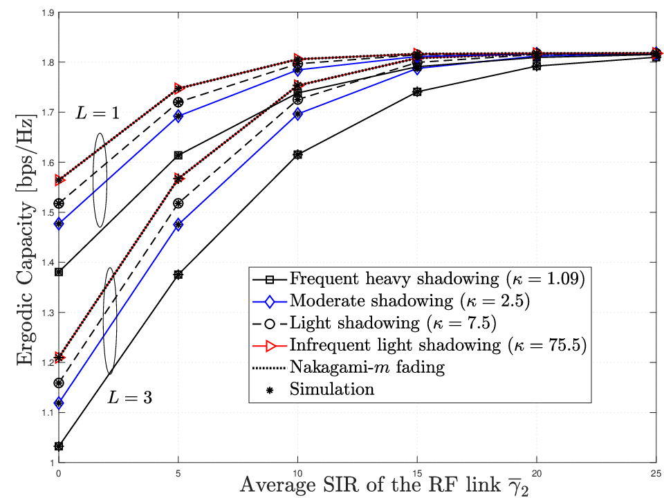
Fig. 6 investigates the effect of shadowing severity on the ergodic capacity of mixed FSO/mmWave CSI-assisted relaying suffering interference. A general observation is that the shadowing degrades the system’s overall performance. Furthermore, it can be inferred from Fig. 6 that as the SIR of the mmWave link increases, a negligible effect of shadowing and interference on the capacity is observed and the performance remains almost the same since the weaker link acts as the dominant link, which is the FSO link in this case. This can be explained by (25). It may be also useful to mention that the ergodic capacity curves of mixed FSO/mmWave under infrequent light shadowing () and mixed Málaga-/Nakagami- systems coincides thereby unambiguously corroborating the much wider scope claimed by our novel analysis framework and the rigor of its mathematical derivations.

Fig. 7 shows the impact of power allocation on the outage probability of mixed FSO/mmWave relay system against dB when dB and dB. Moreover, we investigate the impact of the proposed power allocation formula in (77) on the outage performance and compare it then to the baseline scheme with no power allocation, i.e., , over different mmWave bandwidths. It can be observed that the outage decreases with optimal power allocation compared than with equal power allocation. The achieved gain is of dB at a target outage of . It can be seen from Fig. 7 that the outage decays as the mmWave bandwidth decays.
VII Conclusion
We have studied the performance of relay-assisted mixed FSO/mmWave systems with RF interference and shadowing. The H-transform theory is involved into a unified performance analysis framework featuring closed-form expressions for the outage probability, the BER and the average capacity assuming Málaga-/generalized- channel models for the FSO/shadowed mmWave links while taking into account pointing errors. The diversity order and coding gain are derived for all studied scenarios. Furthermore, we derived an analytical expression for the optimal power allocation at each hop. Main results showed that under weak atmospheric turbulence conditions, the system performance is dominated by the RF channels and a diversity order of is achieved by the system in light shadowing. Otherwise diversity order is affected by the minimum value of the turbulence fading, light shadowing, and pointing error parameters.
VIII Appendix A
Proof of Theorem 1
The CDF of the end-to-end SINR with fixed-gain relaying scheme can be derived as
| (78) |
where and are the FSO link’s CDF and the RF link’s PDF, respectively. Differentiation of (6) over yields as
| (79) | |||||
Substituting (1) and (79) into (78) while resorting to the integral representation of the Fox-H [29, Eq. (1.2)] and Meijer-G [30, Eq. (9.301)] functions yields
| (80) | |||||
where , and and denote the and -planes, respectively. Finally, simplifying to by means of [30, Eqs. (8.380.3) and (8.384.1)] while utilizing the relations , and then [35, Eq. (1.1)] yield (III).
IX Appendix B
Proof of Lemma 1
Resorting to the Mellin-Barnes representation of the bivariate Fox-H function [29, Eq. (2.57)] in (III) yields
where (a) follows from using the definition of the -function shown in [40, Eq. (1.1.1)]. Therefore, by applying [40, Theorem 1.11] to (IX) when yields after some algebraic manipulations
where , , and . Finally applying [30, Eq. (931.5)] completes the proof.
X Appendix C
Proof of Lemma 4
From [41], the average capacity can be computed as
| (87) |
where stands for the complementary MGF (CMGF). The CMGF of the first hop’s SNR under Málaga- distribution with pointing errors is given by [14, Eq. (9)]
| (88) |
Moreover, the Laplace transform of the RF link’s CCDF yields its CMGF after resorting to [30, Eq. (7.813.1)] and [29, Eq. (1.111)] as
| (89) |
Finally, (IV) follows after plugging (88) and (89) into (87) and applying [35, Eq. (2.2)].
References
- [1] X. Ge, S. Tu, G. Mao, C.-X. Wang, and T. Han, “5G ultra-dense cellular networks,” IEEE Wireless Commun., vol. 23, no. 1, pp. 72-79, Feb. 2016
- [2] C. Dehos, J. L. Gonzalez, A. D. Domenico, D. Ktenas, and L. Dussopt, “Millimeter-wave access and backhauling: The solution to the exponential data traffic increase in 5G mobile communications systems?,” IEEE Commun. Mag., vol. 52, no. 9, pp. 88-95, Sep. 2014.
- [3] A. Navas, J. Balsells, J. Paris, M. Vazquez, and A. Notario, “Impact of pointing errors on the performance of generalized atmospheric optical channels,” Opt. Express, vol. 20, no. 11, May 2012.
- [4] M. K. Samimi, S. Sun, and T. S. Rappaport, “Mimo channel modeling and capacity analysis for 5g millimeter-wave wireless systems,” In Proc. European Conference on Antennas and Propagation (EuCAP), pp. 1–5, Apr. 2016.
- [5] M. Dong and T. Kim, “Interference analysis for millimeter-wave networks with geometry-dependent first-order reflections”, IEEE Trans. vehicular technol., vol. 67, no. 12, pp. 12404–12409 Dec. 2018.
- [6] E. Zedini, I. S. Ansari, and M.-S. Alouini, “Performance analysis of mixed Nakagami- and Gamma-Gamma dual-hop FSO transmission systems,” IEEE/OSA Photon. J., vol. 7, no. 1, Feb. 2015.
- [7] S. Anees and M. R. Bhatnagar, “Performance of an amplify-and-forward dual-hop asymmetric RF-FSO communication system,” IEEE/OSA J. Opt. Commun. and Netw., vol. 7, no. 2, pp. 124–135, Feb. 2015.
- [8] G. T. Djordjevic, M. I. Petkovic, A. M. Cvetkovic, and G. K. Karagiannidis, “Mixed RF/FSO relaying with outdated channel state information,” IEEE J. Sel. Areas Commun., vol. 33, no. 9, pp. 1935–1948, Sep. 2015.
- [9] J. Zhang, L. Dai, Y. Zhang, and Z. Wang, “Unified performance analysis of mixed radio frequency/free-space optical dual-hop transmission systems,” IEEE/OSA J. Lightw. Technol., vol. 33, no. 11, pp. 2286–2293, Jun. 2015.
- [10]
L. Kong, W. Xu, L. Hanzo, H. Zhang, C. Zhao, “Performance of a
free-space-optical relay-assisted hybrid RF/FSO system in
generalized -distributed channels,“ IEEE/OSA
Photon. J., vol. 7, no. 5, Oct. 2015.
- [11] E. Soleimani-Nasab and M. Uysal, “Generalized performance analysis of mixed RF/FSO cooperative systems,” IEEE Trans. Wireless Commun., vol. 15, no. 1, pp. 714–727, Jan. 2016.
Performance analysis of mixed free-space optics/radio frequency amplify-and-forward systems with pointing errors“, Institut National de la Recherche Scientifique- Enegrie Materiaux et Telecommunications, 2017.- [12] P. V. Trinh, T. C. Thang, and A. T. Pham, “Mixed mmWave RF/FSO relaying systems over generalized fading channels with pointing errors,” IEEE/OSA Photon. J., vol. 9, no. 1, Feb. 2017.
- [13] M. Hajji and F. El Bouanani, “Performance analysis of mixed Weibull and Gamma-Gamma dual-hop RF/FSO transmission systems,” in Proc. Int. Conf. Wireless Netw. and Mobile Commun., Rabat, Morocco, 1-4 Nov., 2017, pp. 1–5.
- [14] I. Trigui, N. Cherif, and S. Affes, “Relay-assisted mixed FSO/RF systems over Málaga- and - shadowed fading channels,” IEEE Wireless Commun. Lett., vol. 6, no. 5, pp. 682–685, Oct. 2017.
- [15] I. Trigui, N. Cherif, S. Affes, X. Wang, V. Leung, and A. Stéphenne, ”Interference-limited mixed Málaga- and Generalized- dual-hop FSO/RF systems,” IEEE Ann. Int. Symp. Pers., Indoor, and Mobile Radio Commun., Montreal, QC, Canada, 9-13 Oct. 2017, pp. 1–6.
- [16] E. Balti and M. Guizani, “Mixed RF/FSO cooperative relaying systems with co-channel interference,” IEEE Trans. Commun., vol. 66, no. 9, pp. 4014-4027, Sept. 2018.
- [17] N. Cherif, ”
- [18] H. Lei, Z. Dai, I. S. Ansari, K.-H. Park, G. Pan, and M.-S. Alouini, “On secrecy performance of mixed RF-FSO systems,” IEEE/OSA Photon. J., vol. 9, no. 4, Aug. 2017.
On bit error probability and power optimization in multihop millimeter wave relay systems,“ IEEE Access., vol. 6, pp. 3794–3808, Jan. 2018.- [19] H. Arezumand, H. Zamiri-Jafarian, and E. Soleimani-Nasab, “Outage and diversity analysis of underlay cognitive mixed RF-FSO cooperative systems,” IEEE/OSA J. Opt. Commun. Netw., vol. 9, no. 10, pp. 909–920, Oct. 2017.
- [20] L. Yang, M. O. Hasna, and X. Gao, “Performance of mixed RF/FSO with variable gain over generalized atmospheric turbulence channels,” IEEE J. Sel. Areas Commun., vol. 33, no. 9, pp. 1913–1924, Sep. 2015.
- [21] E. Balti, M. Guizani, B. Hamdaoui, and B. Khalfi, “Aggregate hardware impairments over mixed RF/FSO relaying systems with outdated CSI,” IEEE Trans. Commun., vol. 66, no. 3, pp. 1110–1123, Mar. 2018.
- [22] M. R. Akdeniz, Yuanpeng Liu, and et. al., “Millimeter wave channel modeling and cellular capacity evaluation,” IEEE J. Sel. Areas Commun., vol. 32, no. 6, pp. 1164-1179, June 2014.
- [23] T. Bai and R. W. Heath, Jr., “Coverage and rate analysis for millimeter wave cellular networks,” IEEE Trans. Wireless Commun., vol. 14, no. 2, pp. 1100-1114, Feb. 2015.
- [24] N. I. Miridakis, “On the ergodic capacity of underlay cognitive dual-hop af relayed systems under non-identical Generalized- fading channels,” IEEE Commun. Lett., vol. 19, no. 11, pp. 1965–1968, 2015.
- [25] I. Trigui, A. Laourine, S. Affes, and A. Stéphenne, “Performance analysis of mobile radio systems over composite fading/shadowing channels with co-located interference,” IEEE Trans. on Wireless Commun., vol. 8, no. 7, pp. 3448–3453, 2009.
- [26] P. S. Bithas, N. C. Sagias, P. T. Mathiopoulos, G. K. Karagiannidis and A. A. Rontogiannis, “On the performance analysis of digital communications over generalized- fading channels,” in IEEE Communications Letters, vol. 10, no. 5, pp. 353-355, May 2006.
- [27] I. S. Ansari, F. Yilmaz, and M.-S. Alouini, “Performance analysis of free-space optical links over málaga- turbulence channels with pointing errors,” IEEE Trans. Wireless Commun., vol. 15, no. 1, pp. 91–102, Jan. 2016.
- [28] J. M. Garrido-Balsells, A. Jurado-Navas, J. F. Paris, M. Castillo-Vazquez, and A. Puerta-Notario, “Novel formulation of the m model through the Generalized- distribution for atmospheric optical channels,” Opt. Express, vol. 23, no. 5, pp. 6345–6358, 2015.
- [29] A. M. Mathai, R. K. Saxena, and H. J. Haubold, The H-function: theory and applications, Springer Science & Business Media, 2009.
- [30] I. Gradshteyn and I. Ryzhik, “Table of integrals, series, and products,” 1994.
- [31] A. Chelli, K. Kansanen, M. S. Alouini, and I. Balasingham, ”
- [32] X. Wu et al., “60-GHz millimeter-wave channel measurements and modeling for indoor office environments,” IEEE Trans. Antennas Propag., vol. 65, no. 4, pp. 1912-1924, Apr. 2017.
- [33] Y. Azar et al., “28 GHz propagation measurements for outdoor cellular communications using steerable beam antennas in New York city,” in Proc. IEEE Int. Conf. Commun. (ICC), pp. 5143–5147, Jun. 2013.
- [34] T. S. Rappaport, F. Gutierrez, Jr., E. Ben-Dor, J. N. Murdock, Y. Qiao, and J. I. Tamir, “Broadband millimeter-wave propagation measurements and models using adaptive-beam antennas for outdoor urban cellular communications,” IEEE Trans. Antennas Propag., vol. 61, no. 4, pp. 1850-1859, Apr. 2013.
- [35] P. Mittal and K. Gupta, “An integral involving generalized function of two variables,” Proceedings of the Indian Academy of Sciences-Section A, vol. 75, no. 3, pp. 117–123, 1972.
- [36] R. Verma, “On some integrals involving Meijer’s G-fucntion of two variables,” in Proc. Nat. Inst. Sci. India, vol. 39, no. 5/6, 1966, pp. 509-515.
- [37] A. Lapidoth, S. M. Moser and M. A. Wigger, “On the Capacity of Free-Space Optical Intensity Channels,” in IEEE Transactions on Information Theory, vol. 55, no. 10, pp. 4449-4461, Oct. 2009.”
- [11] E. Soleimani-Nasab and M. Uysal, “Generalized performance analysis of mixed RF/FSO cooperative systems,” IEEE Trans. Wireless Commun., vol. 15, no. 1, pp. 714–727, Jan. 2016.
- [38] Z. Ghassemlooy, W. Popoola, and S. Rajbhandari, Optical Wireless Communication, CRC Press, 2012.
- [39] K. Ito and K. Kunisch, “Lagrange multiplier approach to variational problems and applications,” in Advances in Design and Control, Hoboken, NJ, USA: Wiley, 2008.
- [40] A. A. Kilbas, H-transforms: Theory and Applications, CRC Press, 2004.
- [41] I. Trigui, S. Affes, and A. Stéphenne, “Capacity scaling laws in interference-limited multiple-antenna AF relay networks with user scheduling,” IEEE Trans. Commun., vol. 64, no. 8, pp. 3284-3295, Aug. 2016.