Interpretation of Feature Space using Multi-Channel Attentional Sub-Networks

Masanari Kimura

\dagger

Masayuki Tanaka

\dagger,\ddagger

Affiliation:

\dagger

National Institute of Advanced Industrial Science and Technology Affiliation:

\ddagger

Tokyo Institute of Technology

Abstract

Convolutional Neural Networks have achieved impressive results in various tasks, but interpreting the internal mechanism is a challenging problem. To tackle this problem, we exploit a multi-channel attention mechanism in feature space. Our network architecture allows us to obtain an attention mask for each feature while existing CNN visualization methods provide only a common attention mask for all features. We apply the proposed multi-channel attention mechanism to multi-attribute recognition task. We can obtain different attention mask for each feature and for each attribute. Those analyses give us deeper insight into the feature space of CNNs. The experimental results for the benchmark dataset show that the proposed method gives high interpretability to humans while accurately grasping the attributes of the data.

1 Introduction

In recent years, Convolutional Neural Networks (CNNs) have made great achievements in various tasks krizhevsky2012imagenet; karpathy2014large. Despite such success, it is known that an interpretation of the CNNs is difficult for humans. There are various kinds of research to understand the inference mechanism of CNNs to tackle this problem selvaraju2017grad; zhang2018visual; kuwajima2019improving. In particular, ”Visual explanation”, which visualizes the inference mechanism of the CNN, is an important task.

We aim to obtain highly interpretable neural networks using an attention mechanism to acquire features that are important for classifiers. Our main idea is to train sub-networks with multi-channel attention mask for each attribute. The attention mask applied to the sub-network is not common in the feature map but has the same number of channels as the feature map. This multi-channel attention mechanism can reveal which channel in the feature map focuses on which part of the image.

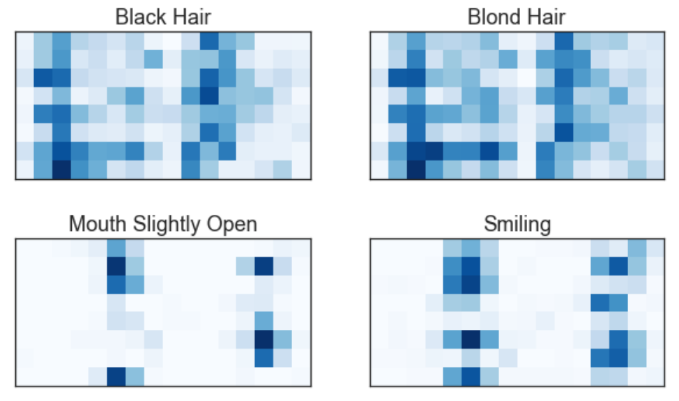
Refer to caption — Figure 1: Average of attention mask of each feature. One element means one-dimensional mean value of attention mask, and there are 128 elements.

Figure 1 shows a grid visualization of the mean values of each channel of attention masks. Our analysis reveals that similar channels of features are commonly used for attributes of ”Black Hair” and ”Blond Hair”. Important channels for attributes of ”Mouth Slightly Open” and ”Smiling” are also similar. This result suggests that the features used for each attribute are limited and can be applied to a very wide range of applications. Our contributions are as follows:

•

We suggest that applying different attention masks to each channel of the feature map which gives us enables deeper insights into CNNs.
•

We propose a novel framework to visualize important features for each attribute by using an attention mechanism.
•

We performed a useful analysis on the features of CNNs using the proposed framework.

Our analysis is highly versatile and leads to a broad range of applied research, such as improvement of classification accuracy, network pruning, image generation, and other applications.

2 Related Works

There are several methods for visualizing important features for CNNs in images selvaraju2017grad; zhang2018visual. Grad-CAM selvaraju2017grad visualizes the area that brings a large gradient to the output neuron when the target class is specified. GAIN zhang2018visual is the framework that provides direct guidance on the attention mask generated by weakly supervised learning. In addition, ABN fukui2018attention made reasoning to CNN using the mechanism of Global Average Pooling (GAP). WiG tanaka2018weighted achieved the performance improvement of CNNs by applying the gating by attention mechanism as the activation function.

In our network architecture, we can obtain an attention mask for each feature while existing CNN visualization methods provide only a common attention mask for all features.

3 Proposed Method

We aim to interpret and theorize the internal mechanisms of CNNs using attention mechanism. Figure 2 shows an overview of our proposed network architecture. In the proposed method, multiple outputs corresponding to an image with multiple attributes.

Let ${\bm{X}}=\{{\bm{x}}_{1},{\bm{x}}_{2},\dots,{\bm{x}}_{n}\}^{N}_{i=1}$ be a sample set, ${\bm{Y}}=\{{\bm{y}}_{1},{\bm{y}}_{2},\dots,{\bm{y}}_{n}\}^{N}_{i=1}$ be a label set, $N$ is the number of samples. The details of each component are as follows.

3.1 Feature Extractor

Feature extractor $f_{f}$ extracts generic feature used by all the following networks. This component performs feature extraction. For this component, we use the Dilation Network fisher2016multi.

3.2 Binary Classifiers with Attention Mechanism

Binary classifiers $F_{b}=\{f_{b}^{1},f_{b}^{2},\dots,f_{b}^{k}\}^{K}_{k=1}$ , where $K$ is number of attributes, are components that perform binary classification corresponding to each attribute of the image. This network is our main component. The loss for the binary classifiers can be expressed by a sum of binary cross entropy of each attribute as

	$\displaystyle L_{b}$	$\displaystyle=$	$\displaystyle-\frac{1}{N}\sum^{N}_{i=1}\sum^{K}_{k=1}y_{i}^{k}\log{\hat{y}_{b,i}^{k}}+(1-y_{i}^{k})\log{(1-\hat{y}_{b,i}^{k})}\,,$
	$\displaystyle\hat{y}_{b,i}^{k}$	$\displaystyle=$	$\displaystyle f_{b}^{k}((1+M^{k}(f_{f}({\bm{x}}_{i})))\otimes f_{f}({\bm{x}}_{i}))\,,$		(2)

where $M^{k}(\cdot)$ is the attention mask for $k$ -th attribute, and $\otimes$ represents element-wise product operation. Note that the attention mask $M^{k}$ has the same number of channels as that of feature $f_{f}$ . It differentiates from existing importance visualization algorithms. We apply attention mask as $1+M^{k}(\cdot)$ to emphasize the area of interest while keeping the low value of the attention mask following in fukui2018attention.

3.3 Multi-Label Classifier

Multi-label classifier is a component that classifies multiple labels. The loss for the multi-label classifier is

	$\displaystyle L_{m}$	$\displaystyle=$	$\displaystyle-\frac{1}{N}\sum^{N}_{i=1}\sum^{K}_{k=1}y_{i}^{k}\log{\hat{y}_{m,i}^{k}}+(1-y_{i}^{k})\log{(1-\hat{y}_{m,i}^{k})}\,,$
	$\displaystyle\hat{y}_{m,i}^{k}$	$\displaystyle=$	$\displaystyle f_{m}^{k}(f_{f}({\bm{x}}_{i}))\,.$		(4)

We put this network component to obtain better feature representation.

3.4 Reconstructor

Reconstructor $f_{r}$ is a component that reconstructs a input image from extracted feature. The reconstruction loss $L_{r}$ is as follows.

L_{r}=\frac{1}{N}\sum^{N}_{i=1}({\bm{x}}_{i}-f_{r}(f_{f}({\bm{x}}_{i})))^{2}\,.

(5)

This component aims to obtain better feature representation $f_{f}(\cdot)$ .

3.5 Overall Loss Function

The overall loss function is:

L=\alpha\cdot L_{b}+\beta\cdot L_{m}+\gamma\cdot L_{r}+\lambda\cdot\|{\bm{M}}\|_{1}\,,

(6)

where, $\alpha$ , $\beta$ , $\gamma$ , and $\lambda$ are weight parameters of each component, and $\|{\bm{M}}\|_{1}$ means L1 sparseness to the attention mask which is used to extract features that are really important for the data.

4 Experimental Results

We evaluate our method using the CelebA dataset liu2015deep, which consists of 40 facial attribute labels and 202,599 images (182,637 training images and 19,962 testing images). The parameters of the proposed method are $\alpha=1$ , $\beta=1$ , $\gamma=4$ and $\lambda=0.00001$ . The dimension of the attention mask and feature map is 128. The reproduction code is available online¹¹ 1 http://www.ok.sc.e.titech.ac.jp/%7Emtanaka/proj/mam/.

Figure 3 shows the visualization of the attention mask by our proposed method. In this figure, common feature channels are visualized for each attribute, and each column means the top three features which have high importance for each attribute. Our attention masks focus on areas that may be important to attributes. In addition, this experimental result suggests that analysis of feature space reveals the relationship among attributes. For example, feature IDs 25, 14 and 50 are not used in Mouse Slightly Open, although they are used in Smiling. On the other hand, IDs 105 and 50 are used in the therapy of Smiling and Mouse Slightly Open, and ID 8 is not used in Smiling. Only the mouth region is focused for the attribute of Mouse Slightly Open, while a wide region including mouse and eyes are focused for the attribute of Smiling. Those results are consistent with the human instinct.

Figure 4 shows the visualization of the correlation of the feature space. Table 1 lists some of the feature IDs and their highly correlated features. Our multi-channel attention mechanism makes it possible to obtain correlations among each channel of the feature map.

Table 2 lists some of the attributes and their highly correlated attributes. Correlations of attributes are estimated based on correlations of features. Attributes that are intuitively similar are highly correlated. This result makes it possible to group highly correlated attributes. In addition, experimental results may even reveal potential relationships among attributes.

Table 3 shows the experimental results of the classification task in the CelebA dataset. In this experiment, MT-RBM PCA ehrlich2016facial, LNets+ANet liu2015deep, and FaceTracer kumar2008facetracer are used as comparison methods. The proposed method achieves good performance with many attributes and all average accuracy.

Table 1: Correlation among the features. It lists the target features, highly correlated features with the target, and correlation.

Target Feature ID	Top5 Highly Correlated Feature IDs
1	72 (0.98)	87 (0.95)	44 (0.94)	92 (0.94)	87 (0.94)
32	111 (0.96)	114 (0.95)	100 (0.95)	15 (0.94)	119 (0.94)
64	127 (0.97)	15 (0.97)	119 (0.97)	114 (0.97)	57 (0.97)

Table 2: Correlation among the attributes. It lists the target attributes and the top five attributes that are highly correlated with the target.

Target Attribute	Top5 Highly Correlated Attributes
Black Hair	Blond Hair, Brown Hair, Bald, Wearing Hat, Gray Hair
Heavy Makeup	Wearing Lipstick, Male, Rosy Cheeks, Attractive, Young
Bushy Eyebrows	Bags Under Eyes, Eyeglasses, Arched Eyebrows, Heavy Makeup, Attractive

Table 3: Classification accuracy on the CelebA dataset. In this experiment, MT-RBM PCA ehrlich2016facial, LNets+ANet liu2015deep, and FaceTracer kumar2008facetracer are used as comparison methods.

Attribute	Ours	ehrlich2016facial	liu2015deep	kumar2008facetracer
5 Shadow	92.85	90	91	85
Arched Eyebrows	81.37	77	79	76
Attractive	80.71	76	81	78
Bags Under Eyes	83.79	81	79	76
Bald	98.30	98	98	89
Bangs	94.10	88	95	88
Big Lips	70.14	69	68	64
Big Nose	83.67	81	78	74
Black Hair	88.39	76	88	70
Blond Hair	95.10	91	95	80
Blurry	95.33	95	84	81
Brown Hair	86.55	83	80	60
Bushy Eyebrows	91.87	88	90	80
Chubby	96.02	95	91	86
Double Chin	96.68	96	92	88
Eyeglasses	98.67	96	99	98
Goatee	96.72	96	95	93
Gray Hair	97.89	97	97	90
Heavy Makeup	89.49	85	90	85
High Cheekbone	86.77	83	87	84
Male	97.38	90	98	91
Mouth Open	93.67	82	92	87
Mustache	96.60	97	95	91
Narrow Eyes	86.38	86	81	82
No Beard	94.87	90	95	90
Oval Face	73.33	73	66	64
Pale Skin	97.67	96	91	83
Pointy Nose	75.62	73	72	68
Recede Hair	93.44	96	89	76
Rosy Cheeks	94.67	94	90	84
Sideburns	97.65	96	96	94
Smiling	92.28	88	92	89
Straight Hair	81.60	80	73	63
Wavy Hair	81.64	72	80	73
Earring	84.61	81	82	73
Hat	98.92	97	99	89
Lipstick	92.52	89	93	89
Necklace	86.37	87	71	68
Necktie	96.30	94	93	86
Young	87.00	81	87	80
Average	92.05	87	87	81

5 Conclusion and Discussion

We proposed a novel network architecture and attention mechanism that can give a visual explanation of CNNs. Our multi-channel attention mechanism makes it possible to obtain correlations among each channel of the feature map. We suggest that analysis of feature maps obtained by the proposed method is highly versatile and lead to a broad range of applied research, such as improvement of classification accuracy, network pruning, image generation, and other applications.

6 Acknowledgements

A part of this paper is based on results obtained from a project commissioned by the New Energy and Industrial Technology Development Organization (NEDO).

References

(1) Max Ehrlich, Timothy J Shields, Timur Almaev, and Mohamed R Amer. Facial attributes classification using multi-task representation learning. In Proceedings of the IEEE Conference on Computer Vision and Pattern Recognition Workshops, pages 47–55, 2016.
(2) Hiroshi Fukui, Tsubasa Hirakawa, Takayoshi Yamashita, and Hironobu Fujiyoshi. Attention branch network: Learning of attention mechanism for visual explanation. arXiv preprint arXiv:1812.10025, 2018.
(3) Andrej Karpathy, George Toderici, Sanketh Shetty, Thomas Leung, Rahul Sukthankar, and Li Fei-Fei. Large-scale video classification with convolutional neural networks. In Proceedings of the IEEE conference on Computer Vision and Pattern Recognition, pages 1725–1732, 2014.
(4) Alex Krizhevsky, Ilya Sutskever, and Geoffrey E Hinton. Imagenet classification with deep convolutional neural networks. In Advances in neural information processing systems, pages 1097–1105, 2012.
(5) Neeraj Kumar, Peter Belhumeur, and Shree Nayar. Facetracer: A search engine for large collections of images with faces. In European conference on computer vision, pages 340–353. Springer, 2008.
(6) Hiroshi Kuwajima, Masayuki Tanaka, and Masatoshi Okutomi. Improving transparency of deep neural inference process. arXiv preprint arXiv:1903.05501, 2019.
(7) Ziwei Liu, Ping Luo, Xiaogang Wang, and Xiaoou Tang. Deep learning face attributes in the wild. In Proceedings of the IEEE international conference on computer vision, pages 3730–3738, 2015.
(8) Ramprasaath R Selvaraju, Michael Cogswell, Abhishek Das, Ramakrishna Vedantam, Devi Parikh, and Dhruv Batra. Grad-cam: Visual explanations from deep networks via gradient-based localization. In Proceedings of the IEEE International Conference on Computer Vision, pages 618–626, 2017.
(9) Masayuki Tanaka. Weighted sigmoid gate unit for an activation function of deep neural network. arXiv preprint arXiv:1810.01829, 2018.
(10) F. Yu and V. Koltun. Multi-scale context aggregation by dilated convolutions. In International Conference on Learning Representations, 2016.
(11) Quan-shi Zhang and Song-Chun Zhu. Visual interpretability for deep learning: a survey. Frontiers of Information Technology & Electronic Engineering, 19(1):27–39, 2018.