Lattices of hydrodynamically interacting flapping swimmersPreprint: Preprint #
Abstract
Fish schools and bird flocks exhibit complex collective dynamics whose self-organization principles are largely unknown. The influence of hydrodynamics on such collectives has been relatively unexplored theoretically, in part due to the difficulty in modeling the temporally long-lived hydrodynamic interactions between many dynamic bodies. We address this through a novel discrete-time dynamical system (iterated map) that describes the hydrodynamic interactions between flapping swimmers arranged in one- and two-dimensional lattice formations. Our 1D results exhibit good agreement with previously published experimental data, in particular predicting the bistability of schooling states and new instabilities that can be probed in experimental settings. For 2D lattices, we determine the formations for which swimmers optimally benefit from hydrodynamic interactions. We thus obtain the following hierarchy: while a side-by-side single-row “phalanx” formation offers a small improvement over a solitary swimmer, 1D in-line and 2D rectangular lattice formations exhibit substantial improvements, with the 2D diamond lattice offering the largest hydrodynamic benefit. Generally, our self-consistent modeling framework may be broadly applicable to active systems in which the collective dynamics is primarily driven by a fluid-mediated memory.
I Introduction
The complex collective dynamics of fish schools and bird flocks have long fascinated physicists, biologists and mathematicians Pavlov and Kasumyan 2000; Bajec and Heppner 2009. In addition to their biological relevance, they are living examples of active systems Cavagna and Giardina 2014; Marchetti et al. 2013; Ramaswamy 2010; Saintillan and Shelley 2013 in which energy input by the individual constituents gives rise to organized collective phenomena. While there has been considerable experimental and theoretical progress in characterizing “dry” active systems (e.g. shaken granular rods Narayan et al. 2007; Kudrolli et al. 2008) and the collective behavior of biological systems at the microscale (e.g. bacterial suspensions Sokolov and Aronson 2009; Wensink et al. 2012; Zhang et al. 2010; Saintillan and Shelley 2008), significantly less is known about the role of hydrodynamic interactions in mediating schooling and flocking behavior in collectives of larger animals. More generally, the influence of inertial fluid flows and the consequent long-lived hydrodynamic interactions on collective behavior remains poorly understood. In contrast to the low Reynolds number (Stokes) regime in which microswimmers operate, fluid-mediated memory could significantly impact animal schools and also nonliving systems dominated by wave-particle interactions. As an example of the latter, oil droplets bouncing on a vertically vibrating fluid bath Bush 2015 are known to exhibit crystal-like bound states Lieber et al. 2007; Eddi et al. 2009 as a result of their coupling through surface waves. We present here a modeling framework for the long-lived hydrodynamic interactions between swimmers, with a view to understanding how their collective dynamics might be mediated by flow-induced forces.
The influence of hydrodynamics on schooling and flocking behavior in biological systems has been the subject of intense debate in the scientific literature. While some analyses of starling cluster flock data Bialek et al. 2012; Attanasi et al. 2014 focus on the behavioral mechanisms behind flocking, a recent analysis Portugal et al. 2014 of flying ibises in V-formations demonstrated coherence of the birds’ wing tip paths, which enables upwash capture from their neighbors to be maximized. Individual fish have been shown to sense and respond to environmental hydrodynamic cues Ristroph et al. 2015, and benefit from external flows by harnessing the energy from vortices Triantafyllou et al. 2000; Liao 2007; Liao et al. 2003. While some studies have argued against a hydrodynamic function for fish schools Partridge and Pitcher 1979 and instead focused on the social interactions between fish Jolles et al. 2017; Swain et al. 2015; Tunstrøm et al. 2013, a number of observations Partridge et al. 1983; Herskin and Steffensen 1998; Marras et al. 2015; Ashraf et al. 2017 have indicated that schooling fish could benefit from hydrodynamic interactions by realizing significant energy savings.
Theoretical models of flocks and schools have also largely ignored hydrodynamic interactions, and instead have shown that self-organized collective behavior may emerge from a relatively simple set of behavioral interaction rules Couzin et al. 2002; Lopez et al. 2012. Examples are the seminal works of Huth & Wissel Huth and Wissel 1992 and Viscek et al. Vicsek et al. 1995, which have been extended to other discrete-time models with more elaborate interaction rules Barberis and Peruani 2016. Far-field hydrodynamic interactions have been recently incorporated into self-propelled particle models of swimmers subject to phenomenological behavioral rules Gazzola et al. 2016; Filella et al. 2018, but such models neglect the vorticity-induced forces thought to be relevant for schooling fish Liao 2007.
Fish schools and bird flocks can exhibit orderly lattice-like formations, although field observations are diverse and sometimes contradictory Pavlov and Kasumyan 2000; Bajec and Heppner 2009. Prior observations revealed that fish schools may adopt lattice configurations in a statistical sense Cullen et al. 1965. A number of fish species (e.g. minnow, bream, saithe, herring) adopt schooling formations reminiscent of 3D tetrahedral and cubic lattices, but others (e.g. cod) adopt less ordered configurations Partridge et al. 1980; Pitcher 1973. Relatively rigid school structures, which are treated in this paper, have also been observed. For example, there are a number of accounts of fish swimming in linear chains Gudger 1944. In their studies of red nose tetra fish, Ashraf et al. Ashraf et al. 2017; Ashraf et al. 2016 noted a prevalence of 2D diamond lattice formations at low swimming speeds and “phalanx” formations at higher speeds, the latter being a side-by-side arrangement of swimmers roughly equispaced in a single line perpendicular to the swimming direction. These two schooling formations have also been observed in bluefin tuna Newlands and Porcelli 2008, for which small schools tend to adopt a phalanx formation while larger schools adopt a diamond lattice. With respect to bird flocks, ibises have been observed to obtain aerodynamic and energetic benefits from in-line formation flight Portugal et al. 2014. Certain species (e.g. pelicans Weimerskirch et al. 2001, Canada geese Badgerow and Hainsworth 1981, ibises Portugal et al. 2014) are thought to benefit from their observed V-formation flight, while it is claimed that others (e.g. pigeons Usherwood et al. 2011, pink-footed geese Cutts and Speakman 1994) do not. Corcoran & Hedrick Corcoran and Hedrick 2019 have recently identified a new type of ordered configuration in shorebird flocks, the “compound V-formation,” wherein a given bird commonly flies roughly one wingspan to the side and to the back from the bird in front of it. Such an ordered structure is observed at all spatial scales within an extended flock, unlike the purely local structure exhibited by starling cluster flocks Bialek et al. 2012; Attanasi et al. 2014.
In an attempt to explain such ordered structures, Weihs’ seminal papers Weihs 1973; Weihs 1975 considered vortex-induced hydrodynamic interactions in a 2D lattice of swimmers. By positing that fish seek to minimize their hydrodynamic drag while avoiding large flow velocity gradients, Weihs argued that a diamond lattice is the energetically optimal arrangement. While this model has been highly influential, it has not been developed further, due to the lack of experimental confirmation and various modeling assumptions. Specifically, the school’s swimming dynamics was not accounted for; hence, the speed and efficiency were not self-consistently calculated, and there was no consideration of the stability of the most efficient state. Moreover, the influence of the streamwise spacing between swimmers was largely neglected, as the swimmers were assumed to be separated by at least five flapping wavelengths. These deficits are addressed through the model we present herein.
Various groups have conducted numerical simulations of the Navier-Stokes equations coupled to an immersed body’s dynamics, and have thus studied flapping wings Streitlien and Triantafyllou 1995; Anderson et al. 1998; Alben et al. 2012; Moore 2017; Akhtar et al. 2007 and deformable bodies with more realistic fish-like kinematics Zhu et al. 2014; Neveln et al. 2014; Tytell et al. 2010; Borazjani and Sotiropoulos 2008; Liu et al. 2017; Gazzola et al. 2011; Hieber and Koumoutsakos 2008; Maertens et al. 2017. Hemelrijk et al. Hemelrijk et al. 2014 and Daghooghi et al. Daghooghi and Borazjani 2015 modeled a fish school by numerically simulating a swimmer with doubly-periodic boundary conditions in 2D and 3D, respectively, and found that swimmers move faster in schools than in isolation. However, neither study examined the dependence of the speed on the streamwise distance between swimmers. While these studies allowed for the complex flow structures around flapping bodies to be quantitatively studied, simulations of fish schools are computationally challenging because of the large Reynolds number of the associated flow and the number of interacting bodies, prohibiting a detailed parametric study of lattice formations.
Understanding the role of hydrodynamic interactions in fish schools may thus benefit from a simplified physical system amenable to theoretical analysis. An example is the recent experimental work of Becker et al. Becker et al. 2015, who realized an in-line formation of swimmers using freely-translating, periodically heaving wings in a cylindrical water tank. They observed that the system exhibited a bistability of “schooling states” and spontaneously locked into either a slow mode or fast mode, the latter of which exhibited a significant speed increase relative to an isolated swimmer. The experiments were extended by Ramananarivo et al. Ramananarivo et al. 2016 to allow tandem swimmers to dynamically select both their speeds and relative positions.
We present here a modeling framework for understanding the hydrodynamic interactions among flapping swimmers at high Reynolds number. Our conceptually simple model is rich enough to incorporate the essential features of the swimmers’ hydrodynamic interactions, while allowing for analytical determination of the model’s exact solutions and their stability properties. Crucially, our model differs from other self-propelled particle models in that the swimmers’ shed vortices are accounted for, so the thrust on a swimmer depends on the system’s history. The swimmers thus interact through a fluid-mediated memory, stored through the collective shed vorticity, and we self-consistently solve for the formation’s emergent speed. The model yields insight into experiments on interacting wings Becker et al. 2015 and predicts instabilities that can be explored in the laboratory. We also extend our model to 2D and determine the lattice formations that allow for the greatest speed and efficiency, thus addressing the questions first posed by Weihs Weihs 1973; Weihs 1975. Specifically, we obtain the following hierarchy: while a phalanx formation (§IV.2) offers a small improvement over a solitary swimmer, 1D in-line (§IV.1) and 2D rectangular lattice formations (§IV.3) exhibit substantial improvements, with the 2D diamond lattice (§IV.4) offering the largest hydrodynamic benefit.
II Simple model of an in-line formation
We first consider the simplest model for a school: an infinite line of swimmers modeled as heaving rigid wings driven periodically with prescribed vertical position , and coupled by nearest-neighbor interactions, as shown in Fig. 1a. We assume the swimmers to be separated by a fixed distance , so the only degree of freedom is the formation’s speed . Our goal is to construct the governing equations for this system, and determine the dependence of on the kinematic parameters and .
The Reynolds number of the flow around the wings used in experiments Becker et al. 2015 is typically large, , where is the chord length and the fluid’s kinematic viscosity. Such a flow is complex and difficult to quantitatively characterize, both experimentally and numerically. We thus make the simplifying assumption that the flow is two-dimensional, inviscid and incompressible, and that the flow structures may be approximated by point vortices shed from the swimmers’ trailing edges at the extrema of their trajectories (Fig. 1b). These vortices mediate the interactions between swimmers. We fix the vortex strength as , where is a free parameter Schnipper et al. 2009; Buchholz et al. 2011. We also assume that the vortex strength decays exponentially over a timescale , an assumption that accounts for turbulent breakdown of vortical structures at high Reynolds number Daghooghi and Borazjani 2015; Ramananarivo et al. 2016; Higdon and Corrsin 1978. Both of these assumptions are discussed in detail in Supplemental Material §II B. We are primarily concerned with trajectories for which the swimming speed is much larger than the characteristic advection speed of vortices Milne-Thomson 1968, , being the distance between vortices of the same sign, and thus assume the vortices to be stationary.
We now construct evolution equations for the swimmers’ position and velocity, with the relevant variables listed in Supplemental Material Table I. Since the swimmers interact through vortices shed by their nearest neighbors, and the distance between them is fixed, the formation’s trajectory is determined by that of a single swimmer. Instead of modeling the swimmer’s continuous-time motion, we evolve its horizontal position and velocity on the midplane at the discrete times , where is the flapping half-period. At each time step, the swimmer sheds a point vortex of positive (negative) circulation at the peak (trough) of its trajectory for odd (even) , which generates the characteristic reverse von Kármán wake Triantafyllou et al. 2000 of a self-propelling swimmer (Fig. 1b, Supplemental Movie 1). The swimmer moves under the influence of two forces: a drag , and a propulsive thrust , where is the fluid vorticity in the complex plane and is the swimmer’s vertical velocity. The equations of motion are thus
| (1) |
the trailing edge of a swimmer centered at the origin is at , and is the swimmer’s effective mass per unit span, defined in Supplemental Material §II. We impose the boundary-layer drag law , where is the fluid density and the drag coefficient. Crucially, the propulsive force depends on the swimmers’ dynamically generated vorticity field .
We compute the propulsive force using the method detailed in Supplemental Material §I. In summary, we model the swimmers as up-down symmetric wings in the complex plane. Such a wing is represented through the action of the so-called Joukowski map on a circle of radius in the -plane, where sets the swimmers’ vertical thickness and roughly sets the chord length. The central vortex strength is obtained by imposing the Kutta condition at the swimmer’s sharp trailing edge , which ensures that the flow remains smooth there. To make the calculation tractable, we assume that the swimmers influence each other only through their shed vortices and not through their body dynamics, an assumption we expect to be valid in the regime . We thus obtain an explicit form for the iterated map (1) that evolves the swimmer’s position and velocity, given in Supplemental Material Eq. (12).
We note that a similar method was used by Ramananarivo et al. Ramananarivo et al. 2016 to calculate the hydrodynamic force on a wing due to shed point vortices. However, that work neglected consideration of the wings’ dynamics, which is explicitly accounted for by our iterated map (1). For this reason, our work goes beyond theirs in two significant ways. First, we are able to assess the stability of steady schooling states, which yields important information about which states are observed experimentally Becker et al. 2015 and thus which lattice configurations are hydrodynamically optimal. Second, we are able to capture time-dependent schooling states, which we find to emerge naturally in 1D flocks (§III). Moreover, while the prior work was limited to a 1D configuration, modeling 2D diamond lattices requires consideration of time-dependent schooling states, as shown in §IV.4.
Our theoretical model for the flow field generated by a flapping wing exhibits satisfactory agreement with Becker et al.’s measurements Becker et al. 2015 using particle image velocimetry, with upstrokes and downstrokes producing upward and downward fluid flows (Supplemental Fig. 1). Our model thus exhibits qualitative similarity with their ad hoc 1D kinematic model (i.e. swimmers’ inertia is neglected and forces directly determine the swimming speed), which posits an interaction force between swimmers that oscillates sinusoidally on the flapping period and also decays in time. However, our model is derived from a detailed physical description of vortex-induced fluid forces, thus permitting quantitative comparison to experimental data (§III) and treatment of 2D formations (§IV). We also explicitly incorporate the swimmers’ inertia, allowing for an assessment of the stability of steady schooling states (§III).
Our considerable simplification of the flow structures allows the formation’s dynamics to be analyzed mathematically. Moreover, simulation of the governing equations is inexpensive, which allows us to assess the dependence of the dynamics on the kinematic parameters and . As shown in Supplemental Material §II, the governing equations can be written in the dimensionless form
| (2) |
where is specified in Supplemental Material Eq. (17).
III Comparison with experiment
We seek steadily translating solutions to Eq. (2) and assess their stability, first with the goal of rationalizing the experimental observations of Becker et al. Becker et al. 2015. The analysis of Eq. (2) is nontrivial due to the temporal nonlocality of the formation’s dynamics: updating the velocity requires knowledge of the swimmer’s history, which is a generic feature of flow-induced interactions at high Reynolds number.
Substituting the steady state into Eq. (2), we find that satisfies the algebraic equation
| (3) |
This equation is solved numerically using a bisection method. The linear stability analysis of such steady state solutions is given in Supplemental Material §III. In summary, we linearize Eq. (2) around the steady state solution, and find the eigenvalues of the linear stability problem using the discrete Laplace transform. We show that the eigenvalues are given by the zeros of the function
| (4) |
where the constants and function are specified in Supplemental Material §III. The steady state solution is stable if all of the roots of lie inside the unit disc in the complex plane, , and is unstable otherwise. We use a numerical contour integration method Delves and Lyness 1966 to find the roots of in the annular region , where is a sufficiently large number. The stability properties of the steady state solution are dictated by the location of the root of that is largest in magnitude.
Figure 2 shows the comparison between theory (curves) and experiment Becker et al. 2015 (triangles) for an in-line formation. In the experiments of Becker et al. Becker et al. 2015, the distance between swimmers is fixed, while the flapping frequency and amplitude are varied. The measured swimming speed is shown in Fig. 2a. The data in Fig. 2b are plotted in terms of the schooling number , which denotes the number of wavelengths separating the swimmers Becker et al. 2015. That is, integer values of indicate trajectories for which the swimmers traverse identical paths, and half-integer values indicate trajectories for which neighboring swimmers traverse paths that are perfectly out-of-phase. The steady state solutions predicted by Eq. (3) are color-coded according to their stability: specifically, blue denotes stable states; red denotes unstable states for which and ; and green denotes oscillatory states, which may destabilize via either a flip bifurcation ( and ) or a Neimark-Sacker bifurcation (). The physical significance of these instabilities is explained at the end of this section.
The theoretical predictions in Fig. 2 exhibit generally excellent agreement with the experimental data of Becker et al. Becker et al. 2015. At the lowest flapping amplitude considered, cm, the agreement between theory and experiment is less good, presumably owing to the breakdown of the point-vortex approximation at low flapping amplitudes. We note that three free parameters, namely, (drag coefficient), (vortex time decay) and (initial vortex strength), are chosen once to best fit all of the experimental data across flapping frequency and amplitude . The numerical values of these parameters exhibit good agreement with results in the existing literature, as detailed in Supplemental Material §II B. Indeed, our fit value seconds compares well with the value seconds inferred from the data of Newbolt et al. (Newbolt et al. 2019, Supporting Information), who measured the temporal decay of the flow generated by a flapping wing in a water tank. Generally, the correspondence between theory and experiment makes clear that our simplified approach to modeling the flow and the swimmers’ dynamics captures the key features of the hydrodynamic interactions between swimmers at high Reynolds number.
The experiments of Becker et al. Becker et al. 2015 provided evidence for the bistability of steady states, and the emergence of coexisting “slow modes” and “fast modes” for the same flapping frequency and amplitude . Our theoretical predictions explain these observations in terms of the stability properties of the steady state solutions. Indeed, branches of stable (blue) solutions are separated by unstable (red) branches, as shown in Fig. 2. Specifically, schooling numbers for are favored by the system when the wings are moving fast due to their large flapping frequency, a regime in which hydrodynamic interactions are the strongest. The unstable branches typically run through schooling numbers , which are thus avoided by the system. The emergence of these schooling numbers is explained analytically in Supplemental Material §II A. We note that the oscillatory structure of the predicted solutions is a consequence of the hydrodynamic coupling between swimmers, as the speed is a monotonically increasing function of the flapping frequency for an isolated swimmer.
In addition to explaining the bistability of steady states, the linear stability analysis in Fig. 2 hints that in-line formations may show unsteady behavior, which is confirmed by numerical simulations of Eq. (2). Specifically, Supplemental Fig. 2a shows a simulation conducted in a parameter regime in which the steady state solution goes unstable via a flip bifurcation, so the swimmer’s velocity oscillates on the flapping period. In experiments, one would thus expect the swimming speed to change appreciably during a single flap, but to be roughly the same at the start of each flap. More interestingly, Supplemental Fig. 2c shows that a steady schooling state may also undergo a Neimark-Sacker bifurcation, in which the swimming speed oscillates over a period long relative to the flapping period, for the parameter regime explored here. Due to its simplicity, our model furnishes testable predictions for the manner in which steady schooling states destabilize, and the parameter regimes in which they do so.
IV Comparative analysis of different formations
Having benchmarked our theoretical model against experimental data, we analyze how hydrodynamic interactions impact the performance of different lattice formations. We consider two performance measures: the formation’s speed and cost of transport , and compare these with the corresponding speed and cost of transport of a single isolated swimmer. The cost of transport is a “gallons-per-mile” measure of efficiency that quantifies the formation’s energy consumption per unit distance Tokić and Yue 2012, where is the instantaneous mechanical power output of the swimmer at time and denotes a time average. A formula for is given in Supplemental Material §IV.
We compute the speed and cost of transport of in-line (§IV.1), phalanx (§IV.2), rectangular lattice (§IV.3), and diamond lattice (§IV.4) formations as a function of the distance between swimmers. Our goal is to identify the lattice formations that maximize the speed and minimize the cost of transport relative to that of a single swimmer, values and indicating a benefit due to collective hydrodynamic interactions. In this section, we restrict our attention to a single representative set of flapping kinematics, Hz and cm, for which and , the low Strouhal number regime being biologically relevant for fish schools Triantafyllou et al. 2000. All distances are reported in units of the swimmer’s approximate body length .
IV.1 In-line formation
We first solve Eq. (3) to find the dependence of the swimming speed on the streamwise distance between swimmers in a line. As in §III, we assume the formation’s dynamics to be dominated by nearest-neighbor interactions in the streamwise direction. The results are shown in Fig. 3. As expected from the discussion in §III, a slow mode () and fast mode () may coexist for a given value of (Fig. 3a). The maximum speedup of 17% corresponds to a state with , while the largest slowdown by 19% corresponds to a state with (Fig. 3b). The lowest cost of transport is and corresponds to a state with , indicating a maximum energy savings of 25%, while the highest cost of transport corresponds to a state with (Fig. 3c). Plotting as a function of (Fig. 3b) shows that states with and typically have the highest speeds, whereas those with and have the lowest. Conversely, Fig. 3c shows that states with typically have the highest cost of transport, whereas those with and have the lowest. Comparing Fig. 3b and 3c, we observe that high-speed states () are typically associated with an increased cost of transport (), indicating a tradeoff between speed and energy consumption.
To understand the oscillatory dependence of on , we derive an approximate form for the thrust and lift on a swimmer due to the vortices shed by its neighbors, assuming that the vortices (with positions and strengths ) are far from the body, . In Supplemental Material §I, we show that
| (5) |
is the vertical velocity of the flow induced by the neighboring swimmers’ shed vortices and is the swimmer’s velocity. Figure 3d shows a schematic of the reverse von Kármán (thrust) wake and associated fluid flow generated by a flapping swimmer. A swimmer moving upward () in its neighbor’s wake would experience a constructive interaction force and thus a speedup () for , and the opposite for , according to Eq. (5). We note that these conclusions may be justified mathematically by adapting the argument in Supplemental Material §II A, in which we derive an approximate form for the interaction force (5) in the biologically-relevant low Strouhal number limit Triantafyllou et al. 2000.
A similar argument may be used to qualitatively understand the tradeoff between speed and cost of transport. A wing moving up () in a high-speed state () experiences a downward flow from its neighbor’s wake (), which implies by Eq. (5). High-speed states are thus typically associated with an increased power consumption, as the wing’s vertical motion is opposed by its neighbor’s induced flow. In the low Strouhal number limit , the increase in cost of transport due to the increased power consumption dominates the decrease in associated with the higher speed, as shown in Supplemental Material §IV A.
We may use the foregoing arguments to draw conclusions about an in-line formation in which the nearest neighbors flap perfectly out-of-phase with respect to each other. For such a configuration, the right-hand sides of the formulae in Eq. (5) for and would simply have their signs reversed. We thus expect a speedup and larger cost of transport for schooling numbers , and a slowdown with lower cost of transport for . That is, Figs. 3b and 3c would be qualitatively unchanged, apart from a shift of the horizontal axis, .

IV.2 Phalanx
Motivated by the experimental observations of Ashraf et al. Ashraf et al. 2017, we now consider a phalanx of swimmers: infinitely many swimmers equally spaced by a distance in the lateral () direction and, following Weihs Weihs 1975, flapping in antiphase with respect to their neighbors, as shown in Fig. 4 and Supplemental Movie 2. As discussed in Supplemental Material §V A, Weihs Weihs 1975 and Stöcker Stöcker 1999 argued that in-phase flapping would result in an increased drag force on the downstream fish, due to the anomalously large induced velocity in the -direction. Such an argument is in agreement with the experimental observations of Ashraf et al. Ashraf et al. 2016 who found that pairs and triplets of red nose tetra fish preferentially flap in antiphase with respect to their lateral neighbors. We also restrict our attention to the parameter regime to ensure that the swimmers do not collide with each other during a flapping cycle.
A straightforward extension of the iterated map presented in §II permits consideration of this formation, as detailed in Supplemental Material §V. Following the procedure detailed in §III, we find that the swimming speed satisfies an algebraic equation of the form (3) with . The interaction function describes the hydrodynamic thrust due to a side-by-side arrangement of swimmers flapping in antiphase, and is defined in Supplemental Material Eq. (41). The solutions to this equation are shown in Fig. 4. The phalanx formation evidently does not exhibit the multi-stability of steady states seen for in-line formations (§IV.1). By generalizing the linear stability analysis of steady state solutions presented in §III, we find that the steady state is stable for all values of . As shown in Fig. 4, the formation exhibits a slight speedup for all values of , with the maximum speedup of roughly 5% occurring when the swimmers are most tightly packed, . However, such a formation also increases the cost of transport by roughly 4%, with the cost of transport decreasing as . Similar to the 1D formations discussed in §IV.1, the phalanx formation exhibits a tradeoff between speed and cost of transport, although both measures exhibit relatively small variations over a range of values .
IV.3 Rectangular lattice
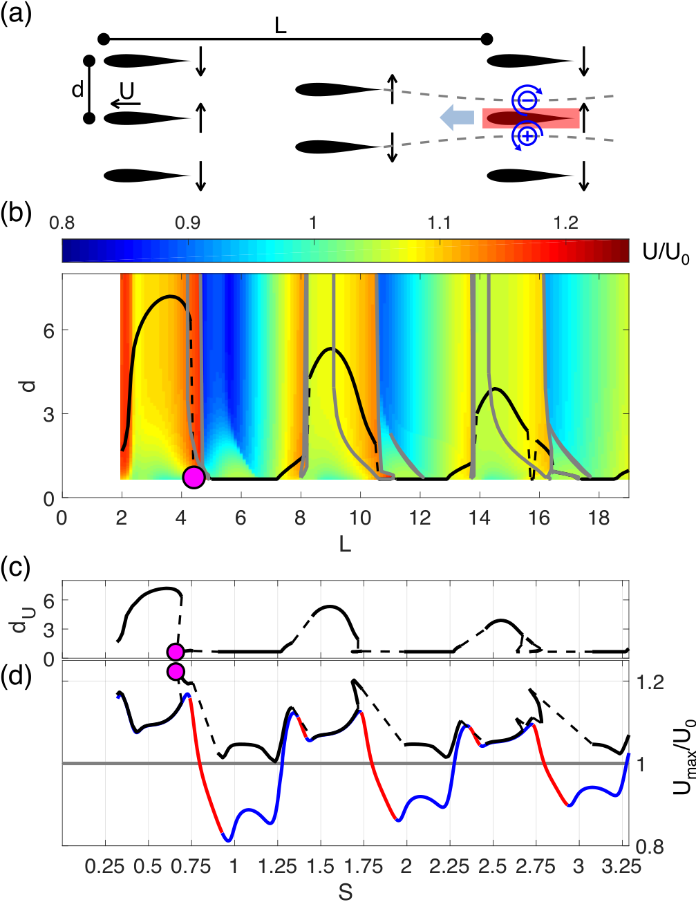
We now consider the rectangular lattice of swimmers shown in Fig. 5a and Supplemental Movie 3: swimmers separated by a streamwise distance and a vertical distance , starting at the positions for . Swimmers flap in phase (antiphase) with respect to their streamwise (lateral) neighbors. As in §II, a swimmer at the origin (red box in Fig. 5a) interacts with the swimmers in the neighboring columns at . Note that the lattice is effectively an in-line formation in the limit . In Supplemental Material §V, we show that the steady speed satisfies the algebraic equation (3), with the function defined in Supplemental Material Eq. (41).
We numerically solve this equation to find the dependence of the steady speed on the geometric parameters and . We then perform numerical simulations of the evolution equations, with initial conditions determined by these steady-state solutions, and compute the trajectory’s time-averaged velocity . Figure 5b shows the normalized velocity as a function of and . As with the in-line formation, there may be multiple steady-state solutions for a given set of parameters; in such cases, we perform multiple simulations and plot the time-averaged speed of the fastest state. The simulations reveal the existence of multiple coexisting states within the regions of geometric parameter space bounded by the gray curves in Fig. 5b. As the lateral distance between swimmers is decreased progressively, these regions of multi-stability typically shrink, but new regions of multi-stability may also emerge.


We find that the formation experiences a maximum speedup of 18% for a roughly square geometry, () and . The black curves in Fig. 5 indicate , the optimal lateral spacing for a given streamwise spacing, and the corresponding speed . Note that, unlike the phalanx (Fig. 4), the greatest speedup is not necessarily achieved by packing the swimmers tightly in the -direction, so is not identically equal to . A comparison between the rectangular lattice and in-line formation is shown in Fig. 5d. The most salient feature is that the slow modes () for an in-line formation all exhibit speedup in the corresponding rectangular lattice with the minimum lateral spacing, . However, the fast modes () for an in-line formation benefit minimally from the rectangular geometry, and the corresponding optimal lateral spacing is often much larger than . Indeed, the fastest rectangular lattice formation is only marginally faster than the fastest in-line formation.
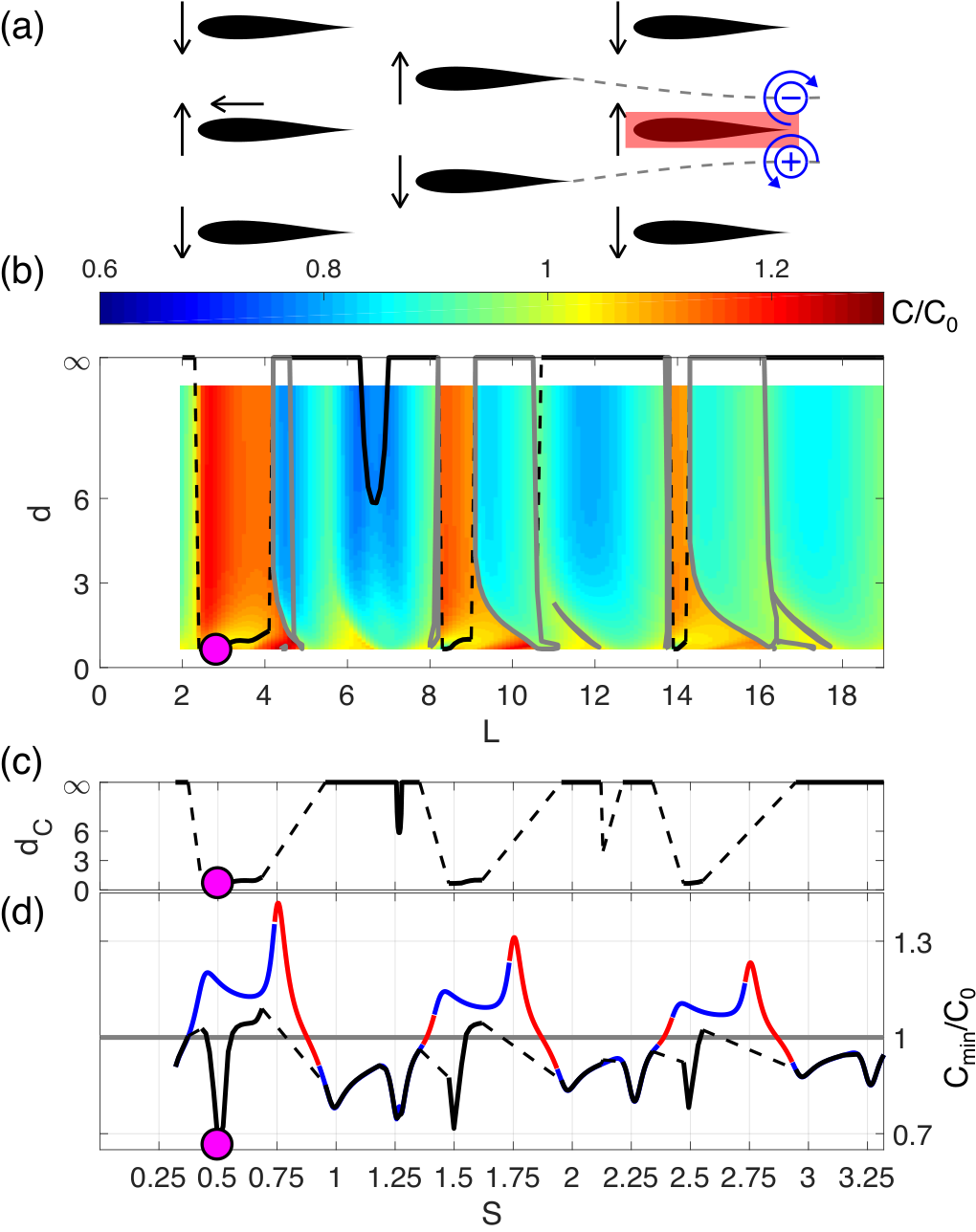
Figure 6 shows the corresponding results for the cost of transport of a rectangular lattice of swimmers. For the regions of parameter space in which multiple states coexist, Fig. 6b shows the cost of transport of the most efficient one. The cost of transport assumes the minimum value for an effectively in-line formation (), for which and (Fig. 3c). The black curves in Fig. 6 correspond to , the optimal lateral spacing for a given streamwise spacing, and the corresponding cost of transport . Unlike , which exhibits a nontrivial dependence on the streamwise spacing (Fig. 5b), typically assumes the values and (Fig. 6b). Figure 6d shows that the states for which typically correspond to inefficient states () for which the rectangular lattice formation affords a slight hydrodynamic advantage over the in-line formation. Conversely, the states for which typically correspond to efficient states () for which the lattice geometry actually increases the cost of transport, making the in-line formation the most efficient.
Taken together, the results in Fig. 5d and Fig. 6d make clear the dominance of streamwise interactions between swimmers in determining both the speed and cost of transport of a rectangular lattice of swimmers. The physical picture given in §IV.1 may thus be used to qualitatively understand how the lattice geometry influences both the speed and cost of transport. Recall that the in-line formation typically experiences a speedup () and a decrease in efficiency () when a swimmer at swims up into the downflow generated by its upstream neighbor at (Fig. 3). For such values of , corresponding to schooling number , the upstream swimmers at in a rectangular lattice contribute an upflow (Fig. 5a), decreasing the thrust but increasing the lift according to Eq. (5). These effects contribute to a decrease in speed but an increase in efficiency for a rectangular lattice as compared to an in-line formation, making it advantageous to increase (decrease) the lateral spacing when optimizing for speed (efficiency). Conversely, the in-line formation is relatively efficient () but slow () for values of corresponding to , the parameter regime in which the upstream swimmers at in the rectangular lattice generate a downflow. This contributes to an increase in speed but a decrease in efficiency, making it advantageous to decrease (increase) the lateral spacing when optimizing for speed (efficiency).
IV.4 Diamond lattice
We now consider the diamond lattice shown in Fig. 7a and Supplemental Movie 4: swimmers separated by a streamwise distance and lateral distance , starting at the positions for and . As in the previous section, swimmers flap in phase (antiphase) with respect to their streamwise (lateral) neighbors, and a swimmer at the origin (red box in Fig. 7a) interacts with the swimmers in the neighboring columns at .
The complete equations are detailed in Supplemental Material Eq. (45). Since the lattice is no longer symmetric about the midplane , the steady state is not a solution to the governing equations, but the period-2 trajectory is. The unknowns and satisfy the pair of algebraic equations
| (6) |
where accounts for the vertical shift in the columns at . This equation describes the balance of drag and vorticity-induced thrust on a swimmer, both of which depend on the swimmer’s instantaneous flapping phase. We describe how to solve these equations numerically, and extend the methodology described in §III to assess the stability of these period–2 solutions, in Supplemental Material §V and §VI, respectively.
We then numerically simulate the governing equations for a diamond lattice with initial conditions determined by the period–2 base states. As with the rectangular lattice described in §IV.3, the simulations reveal the existence of multiple coexisting states, indicated by the regions of parameter space bounded by the gray curves in Fig. 7b. In such cases, Fig. 7b shows the normalized average speedup of the fastest state. We find that the formation experiences a maximum speedup of 22% for and , which corresponds to . As with the rectangular lattice considered in §IV.3, is not identically equal to , although the lateral spacing is indeed minimized for the fastest lattice.
These results may also be qualitatively understood using a simple argument based on fluid flows, and by comparing the diamond lattice and in-line formation in Fig. 7d. As with the rectangular lattice, the slow modes () for an in-line formation exhibit speedup in a diamond lattice with the minimum lateral spacing, . Most fast modes for an in-line formation () benefit minimally from the diamond geometry; however, those with experience a speedup of 3–5% relative to the in-line formation, also with . This is due to the existence of an entirely new branch of fast modes that emerges for , as shown in Supplemental Fig. 3. These fast modes may be attributed to the beneficial dipolar structure generated by the swimmer’s upstream neighbors at , as shown in Fig. 7a. The fluid flow induced by this dipole at the midplane does not have a vertical component, and its horizontal component is negative, effectively imparting additional thrust to the swimmer and increasing its speed. The next flap generates a dipole of opposite sign, which imparts a drag; however, this contribution is weaker than the previous thrust contribution, since the associated vortices are farther from the body.
Figure 8 shows the corresponding results for the cost of transport of a diamond lattice of swimmers. The cost of transport assumes the minimum value for a state with and , indicating that a tightly packed diamond lattice formation realizes a substantial increase in efficiency due to hydrodynamic interactions. Figure 8b shows that, for a given streamwise spacing , the optimal lateral spacing is typically or . This effect is similar to that observed for the rectangular lattice, and may be rationalized by the physical argument presented in §IV.3. However, the diamond lattices for which are noticeably more efficient than their in-line formation counterparts, an effect that is absent for rectangular lattices. This finding may also be explained by the beneficial dipolar structure generated by the swimmer’s upstream neighbors at (Fig. 8a), which provides an additional lift force as the swimmer accelerates upward.
While the distinct optimal diamond lattice formations shown in Fig. 7a and Fig. 8a correspond to stable period-2 states, closer examination of the simulated solutions reveals that they often exhibit a complex nonlinear dynamics. This finding indicates that hydrodynamic interactions may significantly influence schooling behavior when the swimmers are interacting strongly, particularly in the regime . We note that we also observed chaotic solutions in our model for the in-line formation, and leave the complete characterization of the system’s nonlinear dynamics for future work.
V Discussion
We have presented a new model for the hydrodynamic interactions between swimmers in high-Reynolds number flows. While numerical simulations of such systems are computationally challenging, our model offers a simple framework by which to interpret the formation’s dynamics: the swimmers shed vortices during each stroke, and in turn are propelled due to the vorticity-induced flow field. Despite neglecting consideration of the details of the flapping kinematics and the associated flow structures, our model exhibits good agreement with experimental data on interacting wings Becker et al. 2015, while using only three fitting parameters (, and ). As shown in Fig. 2, the observed bistability of slow and fast states is a consequence of overlapping branches of stable (blue) steady-state solutions, which are separated by unstable (red) branches. The multi-stability of states has not been observed in prior theoretical investigations, but is a generic feature of our model: indeed, multiple coexisting states are found in the in-line, rectangular and diamond lattice formations for appropriate values of the geometric parameters. Our model also predicts new schooling instabilities (Supplemental Fig. 2) through which the speed oscillates in time, an effect that can be probed experimentally. Animal schools might employ active control mechanisms in order to mitigate the effects of such instabilities.
Despite the apparent complexity of the hydrodynamic interactions, we show that the interaction thrust force between two swimmers is approximately proportional to the vertical velocity of a swimmer and the vertical velocity of the flow induced by its neighbor (Eq. (5)). This shows that the speed of an in-line formation is sensitive to the streamwise spacing, as a self-propelling flapping swimmer generates a spatially oscillatory flow field in its wake (Fig. 3d). For the set of flapping kinematics considered, we find that an in-line formation may move up to 17% faster than an isolated swimmer, provided the distance between swimmers is such that the schooling number (Fig. 3b). By contrast, a phalanx formation of swimmers flapping in antiphase moves roughly 5% faster than a single swimmer (Fig. 4), with the optimal speedup occurring when the lateral distance between swimmers is minimized. While the fastest rectangular lattice provides a marginal advantage over an in-line formation (Fig. 5), the fastest diamond lattice is able to move 22% faster than a single swimmer (Fig. 7), provided that the lateral distance between swimmers is minimized. This effect may be attributed to the advantageous horizontal flow generated by a swimmer’s upstream neighbors (Fig. 7a).
By using the cost of transport to measure the energetic efficiency, we find that in-line formations may realize an energy savings of 25% over an isolated swimmer, provided the distance between swimmers is such that the schooling number (Fig. 3c). While our finding that the phalanx formation affords a speedup is in agreement with the experimental observations of Ashraf et al. Ashraf et al. 2017, we also find such formations to be slightly less efficient than an isolated swimmer (Fig. 4). Generally, we observe that in-line and phalanx formations exhibit a tradeoff between speed and efficiency. While all rectangular lattices have a higher cost of transport than the most efficient in-line formation (Fig. 6), the most efficient diamond lattice has an energy savings of 33% over an isolated swimmer, an effect that can also be attributed to the effective vortex dipole generated by the swimmer’s upstream neighbors (Fig. 8a). Taken together, our results show that the fastest and most efficient diamond lattice formations are distinct, and that they outperform the other geometries in speed and efficiency, respectively. Based on the argument presented at the end of §IV.1, we expect qualitatively similar results for a model in which the swimmers flap perfectly out-of-phase with respect to their streamwise neighbors in both in-line and 2D lattice formations. While most of the relevant schooling numbers will be shifted, , we still expect the diamond lattices with to be particularly efficient (Fig. 8d), owing to the vortex dipole shed by a swimmer’s upstream neighbors.
Our finding that the most efficient state is realized by a diamond lattice with the minimal lateral spacing is consistent with the results of Weihs Weihs 1973; Weihs 1975. However, our results differ in that the curves and (black curves in Fig. 7d and Fig. 8d, respectively) are not monotonic, implying that there is not an optimal lattice angle. While Weihs argued that it is disadvantageous for a swimmer to swim directly behind another, we find that this is not necessarily the case (Fig. 3). We note that our model differs from Weihs’ in some important ways. First, we model flapping swimmers, and find that the formation’s speed is influenced by the relationship between the swimmer’s kinematics and oncoming fluid flow (§IV.1). More sophisticated computational models Maertens et al. 2017; Verma et al. 2018 of fish-like swimming have also highlighted the importance of this relationship. Second, we allow the vortex strength to decay in our model, which sets an effective interaction distance between swimmers. Third, we explicitly account for the formation’s dynamics and thus the schooling modes’ stability, which was not possible in Weihs’ framework.
Our results may also be compared with recent theoretical and computational studies of a swimmer in a doubly periodic domain, which generates a lattice of swimmers flapping in phase. Recently, Hemelrijk et al. Hemelrijk et al. 2014 conducted 2D numerical simulations using a multi-particle collision dynamics model and also found that the diamond lattice provides the largest speedup relative to a single swimmer (), but that the maximum occurred for , the largest lateral spacing considered. Similarly, the diamond lattice for was found to have the highest Froude efficiency, or the ratio of the useful power to the total power input. However, Hemelrijk et al. Hemelrijk et al. 2014 did not consider the influence of the streamwise spacing , which we find to play a dominant role. Daghooghi & Borazjani Daghooghi and Borazjani 2015 conducted 3D large eddy simulations of rectangular lattices of swimmers at high Reynolds number. They found that the swimming speed and efficiency increase as the lateral distance decreases, but also did not consider the influence of the streamwise spacing and instead fixed . They attributed the observed hydrodynamic advantage to channeling or wake blockage; this effect is beyond the scope of our model, since we assume the vortices to remain in place once shed. Nevertheless, in our simulations of rectangular lattices of swimmers that flap in antiphase with respect to their lateral neighbors, we find that the swimming speed and efficiency do not necessarily exhibit a monotonic dependence on , but instead are nontrivially influenced by both and (Fig. 5b and Fig. 6b). Tsang & Kanso Tsang and Kanso 2013 proposed a far-field hydrodynamic model of swimmers as finite-sized vortex dipoles, and found that swimmers in both rectangular and diamond lattices actually move slower than they would in isolation. They attributed this result to the absence of shed vorticity in their model, which has been shown to mediate the near-field interactions between swimmers Ramananarivo et al. 2016. Our dynamical model builds on these studies by explicitly modeling both the flapping kinematics and shedding of vortices. The model’s mathematical simplicity allows us to analytically show the multi-stability of states in in-line, rectangular and diamond lattice formations, a result absent from all of the studies described above. Moreover, the model’s computational tractability allows us to conclusively determine the dependence of the speed and cost of transport on the geometric parameters and .
We now compare some of our results to schooling formations reported in the literature, despite the current sparsity of quantitative data. In their observations of red nose tetra fish, Ashraf et al. Ashraf et al. 2017; Ashraf et al. 2016 reported that high-speed schools typically adopt phalanx formations with nearest neighbors separated by 0.5–0.6 body lengths. This observation is consistent with our theoretical prediction that the fastest phalanx formation is realized for the minimum lateral distance considered, body lengths (Fig. 4). Similarly, Atlantic bluefin tuna have been observed to adopt phalanx formations with an average lateral spacing between 1 and 1.5 body lengths Newlands and Porcelli 2008; Partridge et al. 1983. When in relatively large schools, this fish species has also been observed to adopt diamond lattice-like formations with a mean first- and second-nearest neighbor separation angle between and (Fig. 5 in Partridge et al. 1983). This observation is roughly consistent with our theoretical prediction that the diamond lattice with the lowest cost of transport has a separation angle of 13∘ (Fig. 8). However, the red nose tetra fish has been observed to adopt diamond lattice formations with a typical separation angle of approximately (Fig. 2b in Ashraf et al. 2017). Moreover, this fish species tends to adopt the phalanx over the diamond lattice formation at high swimming speeds Ashraf et al. 2017, an observation that runs counter to our prediction that the fastest and most efficient states are realized by diamond lattice formations. We note that the spatial phase synchronization between neighboring fish, as measured through the schooling number , is not typically reported, which prevents further quantitative comparison between our theoretical predictions and field observations. Such detailed comparison against biological swimmers would also benefit from more accurate modeling of the swimming kinematics and body shape. Considerations beyond hydrodynamics, such as social cues and predator avoidance, undoubtedly also impact the structure of schools observed in nature.
We expect the results presented herein to be most relevant for understanding fish schools, since we neglected the influence of lift forces on the dynamics. While a recent study of shorebird flocks found no evidence of temporal or spatial phase synchronization between birds Corcoran and Hedrick 2019, ibis flocks were observed to preferentially assume V-formations with median schooling number , and in-line formations with (Supplemental Fig. 2 in Portugal et al. 2014). Extensions of our model might shed light on these phenomena, for which lift generation is an important consideration Higdon and Corrsin 1978. We also note that a conceptually similar iterated map model may readily be applied to 3D flocks and schools; however, new techniques would be required to capture fully 3D dynamics, since the complex-variable techniques used herein cannot simply be extended to calculate the vortex-induced flow and associated forces on the bodies. Our work may also have limited application to “disordered” schools and cluster flocks, which deviate significantly from ordered lattice formations. The model may be generalized to allow for more general body kinematics, including pitching, turning and adaptive spacing between swimmers Ramananarivo et al. 2016; Newbolt et al. 2019.
While the quantitative results presented in this paper depend on the model parameters used, our reduced modeling framework may be applied to understand temporally long-lived hydrodynamic interactions in active systems. Indeed, models for the pilot-wave dynamics of droplets bouncing on a vibrating fluid bath have a similar mathematical structure Bush 2015, and may be extended to probe the droplet’s complex collective dynamics Lieber et al. 2007; Eddi et al. 2009. Generally, we expect models of the type described herein to be broadly applicable to systems of active particles interacting via their collective histories.
Acknowledgements.
We thank Hassan Masoud, Fang Fang, Joel Newbolt, Sophie Ramananarivo and Stephen Childress for helpful discussions. A. U. O. acknowledges support from the Simons Foundation (Collaboration Grant for Mathematicians, award #587006), L. R. acknowledges support from the NSF (DMS-1847955), and M. J. S. thanks the Lilian and George Lyttle Chair of Applied Mathematics.References
- Pavlov and Kasumyan [2000] D. S. Pavlov and A. O. Kasumyan. Patterns and mechanisms of schooling behavior in fish: A review. J. Ichthyology, 40:S163–S231, 2000.
- Bajec and Heppner [2009] I. L. Bajec and F. H. Heppner. Organized flight in birds. Animal Behaviour, 78:777–789, 2009.
- Cavagna and Giardina [2014] A. Cavagna and I. Giardina. Bird flocks as condensed matter. Annual Review of Condensed Matter Physics, 5:183–207, 2014.
- Marchetti et al. [2013] M. C. Marchetti, J. F. Joanny, S. Ramaswamy, T. B. Liverpool, J. Prost, M. Rao, and R. A. Simha. Hydrodynamics of soft active matter. Reviews of Modern Physics, 85(1143), 2013.
- Ramaswamy [2010] S. Ramaswamy. The mechanics and statistics of active matter. Annual Review of Condensed Matter Physics, 1:323–345, 2010.
- Saintillan and Shelley [2013] D. Saintillan and M. J. Shelley. Active suspensions and their nonlinear models. Comptes Rendus Physique, 14:497–517, 2013.
- Narayan et al. [2007] V. Narayan, S. Ramaswamy, and N. Menon. Long-lived giant number fluctuations in a swarming granular nematic. Science, 317(5834):105–108, 2007.
- Kudrolli et al. [2008] A. Kudrolli, G. Lumay, D. Volfson, and L. S. Tsimring. Swarming and swirling in self-propelled polar granular rods. Physical Review Letters, 100(058001), 2008.
- Sokolov and Aronson [2009] A. Sokolov and I. S. Aronson. Reduction of viscosity in suspension of swimming bacteria. Physical Review Letters, 103(148101), 2009.
- Wensink et al. [2012] H. H. Wensink, J. Dunkel, S. Heidenreich, K. Drescher, R. E. Goldstein, H. Löwen, and J. M. Yeomans. Meso-scale turbulence in living fluids. Proceedings of the National Academy of Sciences, 109(36):14308–14313, 2012.
- Zhang et al. [2010] H. P. Zhang, A. Be’er, E.-L. Florin, and H. L. Swinney. Collective motion and density fluctuations in bacterial colonies. Proceedings of the National Academy of Sciences, 107(31):13626–13630, 2010.
- Saintillan and Shelley [2008] D. Saintillan and M. J. Shelley. Instabilities and pattern formation in active particle suspensions: Kinetic theory and continuum simulations. Physical Review Letters, 100(178103), 2008.
- Bush [2015] J. W. M. Bush. Pilot-wave hydrodynamics. Ann. Rev. Fluid Mech., 47, 2015.
- Lieber et al. [2007] S. I. Lieber, M. C. Hendershott, A. Pattanaporkratana, and J. E. Maclennan. Self-organization of bouncing oil drops: two-dimensional lattices and spinning clusters. Phys. Rev. E, 75(056308), 2007.
- Eddi et al. [2009] A. Eddi, A. Decelle, E. Fort, and Y. Couder. Archimedean lattices in the bound states of wave interacting particles. EPL, 87(56002), 2009.
- Bialek et al. [2012] W. Bialek, A. Cavagna, I. Giardina, T. Mora, E. Silvestri, M. Viale, and A. M. Walczak. Statistical mechanics for natural flocks of birds. PNAS, 109(13):4786–4791, 2012.
- Attanasi et al. [2014] A. Attanasi, A. Cavagna, L. Del Castello, I. Giardina, T. S. Grigera, A. Jelić, S. Melillo, L. Parisi, O. Pohl, E. Shen, and M. Viale. Information transfer and behavioural inertia in starling flocks. Nature Physics, 10:691–696, 2014.
- Portugal et al. [2014] S. J. Portugal, T. Y. Hubel, J. Fritz, S. Heese, D. Trobe, B. Voelkl, S. Hailes, A. M. Wilson, and J. R. Usherwood. Upwash exploitation and downwash avoidance by flap phasing in ibis formation flight. Nature, 505:399–402, 2014.
- Ristroph et al. [2015] L. Ristroph, J. C. Liao, and J. Zhang. Lateral line layout correlates with the differential hydrodynamic pressure on swimming fish. Physical Review Letters, 114(018102), 2015.
- Triantafyllou et al. [2000] M. S. Triantafyllou, G. S. Triantafyllou, and D. K. P. Yue. Hydrodynamics of fishlike swimming. Annual Review of Fluid Mechanics, 32:33—53, 2000.
- Liao [2007] J. C. Liao. A review of fish swimming mechanics and behaviour in altered flows. Phil. Trans. R. Soc. B, 362:1973–1993, 2007.
- Liao et al. [2003] J. C. Liao, D. N. Beal, G. V. Lauder, and M. S. Triantafyllou. Fish exploiting vortices decrease muscle activity. Science, 302:1566–1569, 2003.
- Partridge and Pitcher [1979] B. L. Partridge and T. J. Pitcher. Evidence against a hydrodynamic function for fish schools. Nature, 279:418–419, 1979.
- Jolles et al. [2017] J. W. Jolles, N. J. Boogert, V. H. Sridhar, I. D. Couzin, and A. Manica. Consistent individual differences drive collective behavior and group functioning of schooling fish. Current Biology, 27:2862–2868, 2017.
- Swain et al. [2015] D. T. Swain, I. D. Couzin, and N. E. Leonard. Coordinated speed oscillations in schooling killifish enrich social communication. Journal of Nonlinear Science, 25(5):1077–1109, 2015.
- Tunstrøm et al. [2013] K. Tunstrøm, Y. Katz, C. C. Ioannou, C. Huepe, M. J. Lutz, and I. D. Couzin. Collective states, multistability and transitional behavior in schooling fish. PLOS Computational Biology, 9(2):e1002915, 2013.
- Partridge et al. [1983] B. L. Partridge, J. Johansson, and J. Kalish. The structure of schools of giant bluefin tuna in Cape Cod Bay. Environmental Biology of Fishes, 9(3–4):253–262, 1983.
- Herskin and Steffensen [1998] J. Herskin and J. F. Steffensen. Energy savings in sea bass swimming in a school: measurements of tail beat frequency and oxygen consumption at different swimming speeds. Journal of Fish Biology, 53:366–376, 1998.
- Marras et al. [2015] S. Marras, S. S. Killen, J. Lindström, D. J. McKenzie, J. F. Steffensen, and P. Domenici. Fish swimming in schools save energy regardless of their spatial position. Behavioral Ecology and Sociobiology, 69:219–226, 2015.
- Ashraf et al. [2017] I. Ashraf, H. Bradshaw, T-T. Ha, J. Halloy, R. Godoy-Diana, and B. Thiria. Simple phalanx pattern leads to energy saving in cohesive fish schooling. PNAS, 114(36):9599–9604, 2017.
- Couzin et al. [2002] I. D. Couzin, J. Krause, R. James, G. D. Ruxton, and N. R. Franks. Collective memory and spatial sorting in animal groups. Journal of Theoretical Biology, 218:1–11, 2002.
- Lopez et al. [2012] U. Lopez, J. Gautrais, I. D. Couzin, and G. Theraulaz. From behavioural analyses to models of collective motion in fish schools. Interface Focus, 218:1–11, 2012.
- Huth and Wissel [1992] A. Huth and C. Wissel. The simulation of the movement of fish schools. Journal of Theoretical Biology, 156:365–385, 1992.
- Vicsek et al. [1995] T. Vicsek, A. Czirók, E. Ben-Jacob, I. Cohen, and O. Shochet. Novel type of phase transition in a system of self-driven particles. Physical Review Letters, 75(6), 1995.
- Barberis and Peruani [2016] L. Barberis and F. Peruani. Large-scale patterns in a minimal cognitive flocking model: Incidental leaders, nematic patterns, and aggregates. Physical Review Letters, 117(248001), 2016.
- Gazzola et al. [2016] M. Gazzola, A. A. Tchieu, D. Alexeev, A. de Brauer, and P. Koumoutsakos. Learning to school in the presence of hydrodynamic interactions. Journal of Fluid Mechanics, 789:726–749, 2016.
- Filella et al. [2018] A. Filella, F. Nadal, C. Sire, E. Kanso, and C. Eloy. Model of collective fish behavior with hydrodynamic interactions. Physical Review Letters, 120(198101), 2018.
- Cullen et al. [1965] J. M. Cullen, E. Shaw, and H. A. Baldwin. Methods for measuring the three-dimensional structure of fish schools. Animal Behaviour, 13(4):534–536, 1965.
- Partridge et al. [1980] B. L. Partridge, T. Pitcher, J. M. Cullen, and J. Wilson. The three-dimensional structure of fish schools. Behav. Ecol. Sociobiol., 6:277–288, 1980.
- Pitcher [1973] T. J. Pitcher. The three-dimensional structure of schools in the minnow, phoxinus phoxinus (l.). Animal Behaviour, 21:673–686, 1973.
- Gudger [1944] E. W. Gudger. Fishes that swim heads to tails in single file. Copeia, 1944(3):152–154, 1944.
- Ashraf et al. [2016] I. Ashraf, R. Godoy-Diana, J. Halloy, B. Collignon, and B. Thiria. Synchronization and collective swimming patterns in fish (hemigrammus bleheri). J. R. Soc. Interface, 13(20160734), 2016.
- Newlands and Porcelli [2008] K. Newlands and T. A. Porcelli. Measurement of the size, shape and structure of Atlantic bluefin tuna schools in the open ocean. Fisheries Research, 91:42–55, 2008.
- Weimerskirch et al. [2001] H. Weimerskirch, J. Martin, Y. Clerquin, P. Alexandre, and S. Jiraskova. Energy saving in flight formation. Nature, 413:697–698, 2001.
- Badgerow and Hainsworth [1981] J. P. Badgerow and F. R. Hainsworth. Energy savings through formation flight? a re-examination of the vee formation. J. Theor. Biol., 93:41–52, 1981.
- Usherwood et al. [2011] J. R. Usherwood, M. Stavrou, J. C. Lowe, K. Roskilly, and A. M. Wilson. Flying in a flock comes at a cost in pigeons. Nature, 474:494–497, 2011.
- Cutts and Speakman [1994] C. J. Cutts and J. R. Speakman. Energy savings in formation flight of pink-footed geese. J. Exp. Biol., 189:251–261, 1994.
- Corcoran and Hedrick [2019] A. J. Corcoran and T. L. Hedrick. Compound-V formations in shorebird flocks. eLife, 8(e45071), 2019.
- Weihs [1973] D. Weihs. Hydromechanics of fish schooling. Nature, 241, 1973.
- Weihs [1975] D. Weihs. Some hydrodynamical aspects of fish schooling. In T. Y. Wu, C. J. Brokaw, and C. Brennen, editors, Swimming and Flying in Nature, pages 703–718. Springer, 1975.
- Streitlien and Triantafyllou [1995] K. Streitlien and M. S. Triantafyllou. Force and moment on a Joukowski profile in the presence of point vortices. AIAA, 33(4):603–610, 1995.
- Anderson et al. [1998] J. M. Anderson, K. Streitlien, D. S. Barrett, and M. S. Triantafyllou. Oscillating foils of high propulsive efficiency. J. Fluid Mech., 360:41–72, 1998.
- Alben et al. [2012] S. Alben, C. Witt, T. V. Baker, E. Anderson, and G. V. Lauder. Dynamics of freely swimming flexible foils. Physics of Fluids, 24(051901), 2012.
- Moore [2017] M. N. J. Moore. A fast Chebyshev method for simulating flexible-wing propulsion. Journal of Computational Physics, 345:792–817, 2017.
- Akhtar et al. [2007] I. Akhtar, R. Mittal, G. V. Lauder, and E. Drucker. Hydrodynamics of a biologically inspired tandem flapping foil configuration. Theoretical and Computational Fluid Dynamics, 21(3):155–170, 2007.
- Zhu et al. [2014] X. Zhu, G. He, and X. Zhang. Flow-mediated interactions between two self-propelled flapping filaments in tandem configuration. Physical Review Letters, 113(238105), 2014.
- Neveln et al. [2014] I. D. Neveln, R. Bale, A. P. S. Bhalla, O. M. Curet, N. A. Patankar, and M. A. MacIver. Undulating fins produce off-axis thrust and flow structures. Journal of Experimental Biology, 217:201–213, 2014.
- Tytell et al. [2010] E. D. Tytell, C-Y. Hsu, T. L. Williams, A. H. Cohen, and L. J. Fauci. Interactions between internal forces, body stiffness, and fluid environment in a neuromechanical model of lamprey swimming. PNAS, 107(46):19832–19837, 2010.
- Borazjani and Sotiropoulos [2008] I. Borazjani and F. Sotiropoulos. Numerical investigation of the hydrodynamics of carangiform swimming in the transitional and inertial flow regimes. Journal of Experimental Biology, 211:1541–1558, 2008.
- Liu et al. [2017] G. Liu, Y. Ren, H. Dong, O. Akanyeti, J. C. Liao, and G. V. Lauder. Computational analysis of vortex dynamics and performance enhancement due to body-fin and fin-fin interactions in fish-like locomotion. Journal of Fluid Mechanics, 829:65–88, 2017.
- Gazzola et al. [2011] M. Gazzola, P. Chatelain, W. M. van Rees, and P. Koumoutsakos. Simulations of single and multiple swimmers with non-divergence free deforming geometries. Journal of Computational Physics, 230:7093–7114, 2011.
- Hieber and Koumoutsakos [2008] S. E. Hieber and P. Koumoutsakos. An immersed boundary method for smoothed particle hydrodynamics of self-propelled swimmers. Journal of Computational Physics, 227:8636–8654, 2008.
- Maertens et al. [2017] A. P. Maertens, A. Gao, and M. S. Triantafyllou. Optimal undulatory swimming for a single fish-like body and for a pair of interacting swimmers. Journal of Fluid Mechanics, 813:301–345, 2017.
- Hemelrijk et al. [2014] C. K. Hemelrijk, D. A. P. Reid, H. Hildenbrandt, and J. T. Padding. The increased efficiency of fish swimming in a school. Fish and Fisheries, 16(3), 2014.
- Daghooghi and Borazjani [2015] M. Daghooghi and I. Borazjani. The hydrodynamic advantages of synchronized swimming in a rectangular pattern. Bioinspiration and Biomimetics, 10(056018), 2015.
- Becker et al. [2015] A. D. Becker, H. Masoud, J. W. Newbolt, M. Shelley, and L. Ristroph. Hydrodynamic schooling of flapping swimmers. Nat. Commun., 6(8514), 2015.
- Ramananarivo et al. [2016] S. Ramananarivo, F. Fang, A. Oza, J. Zhang, and L. Ristroph. Flow interactions lead to orderly formations of flapping wings in forward flight. Phys. Rev. Fluids, 1(071201(R)), 2016.
- Schnipper et al. [2009] T. Schnipper, A. Andersen, and T. Bohr. Vortex wakes of a flapping foil. J. Fluid Mech., 633:411–423, 2009.
- Buchholz et al. [2011] J. H. J. Buchholz, M. A. Green, and A. J. Smits. Scaling the circulation shed by a pitching panel. J. Fluid Mech., 688:591–601, 2011.
- Higdon and Corrsin [1978] J. J. L. Higdon and S. Corrsin. Induced drag of a bird flock. The American Naturalist, 112(986):727–744, 1978.
- Milne-Thomson [1968] L. M. Milne-Thomson. Theoretical Hydrodynamics, 5th edition. Dover Publications, 1968.
- Delves and Lyness [1966] L. M. Delves and J. N. Lyness. A numerical method for locating the zeros of an analytic function. Mathematics of Computation, 21(100):543–560, 1966.
- Newbolt et al. [2019] J. W. Newbolt, J. Zhang, and L. Ristroph. Flow interactions between uncoordinated flapping swimmers give rise to group cohesion. Proc. Natl. Acad. Sci., 116(7):2419–2424, 2019.
- Tokić and Yue [2012] G. Tokić and D. K. P. Yue. Optimal shape and motion of undulatory swimming organisms. Proceedings of the Royal Society B, 279:3065–3074, 2012.
- Stöcker [1999] S. Stöcker. Models for tuna school formation. Mathematical Biosciences, 156:167–190, 1999.
- Verma et al. [2018] S. Verma, G. Novati, and P. Koumoutsakos. Efficient collective swimming by harnessing vortices through deep reinforcement learning. PNAS, 115(23):5849–5854, 2018.
- Tsang and Kanso [2013] A. C. H. Tsang and E. Kanso. Dipole interactions in doubly periodic domains. Journal of Nonlinear Science, 23(6):971–991, 2013.