MDP-Based Scheduling Design for Mobile-Edge Computing Systems with Random User ArrivalThis work was supported in part by National Natural Science Foundation of China under Grants 61771232 and 91838301, and in part by the Shenzhen Science and Technology Innovation Committee under Grant JCYJ20160331115457945.

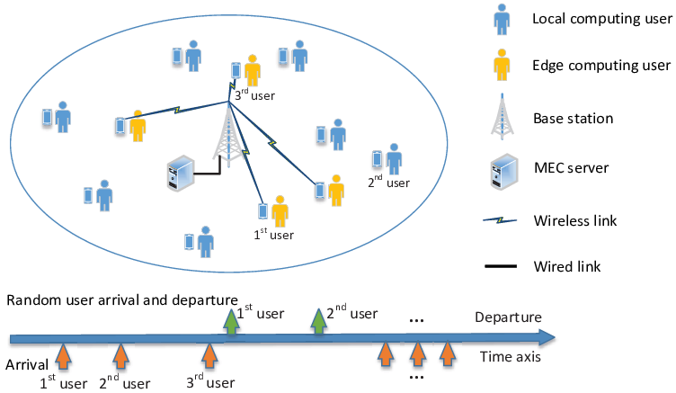
We consider an MEC system as illustrated in Fig. 1, where a BS serves a region $\mathcal{C}$ and an MEC server is connected with the BS. Mobile devices with computation tasks arrive randomly in the service region $\mathcal{C}$. Binary computation offloading model is adopted, and every task is assumed to be indivisible in the sense of computing. Each task can be either computed locally or offloaded to the MEC server via uplink transmission.

There are a number of mobile devices in the cell region $\mathcal{C}$, which may be quasi-static, moving inside or out of the region $\mathcal{C}$. The mobile devices with computation tasks are named as active devices in the remainder of this paper. The time axis of computation and uplink transmission scheduling is organized by frames, each with a time duration $T_{s}$. In each frame, there is at most one new active device arrived in the cell with probability $P_{N}\in(0,1]$. We have no restriction on the distribution and mobility model of the mobile devices in the cell. Instead, the distribution density of the new active device is represented as $\lambda({\mathbf{l}})$ for arbitrary location in the cell region ${\mathbf{l}}\in\mathcal{C}$. Thus, $\int_{\mathcal{C}}\lambda({\mathbf{l}})ds({\mathbf{l}})=1,$ and

Moreover, it is assumed that the location of each active device is quasi-statistic in the cell when its task is being transmitted to the MEC server. The active devices become inactive when their computation tasks have been completed either locally or remotely at the MEC server.

Every new active device in the cell is assigned with a unique index. Let $\mathcal{U}_{L}(t)$ and $\mathcal{U}_{E}(t)$ be the sets of active devices in the $t$-th frame whose tasks are computed locally and at the MEC server respectively, $\mathcal{D}_{L}(t)\subseteq\mathcal{U}_{L}(t)$ and $\mathcal{D}_{E}(t)\subseteq\mathcal{U}_{E}(t)$ be the subsets of active devices whose computation tasks are accomplished in the $t$-th frame locally and at the MEC server respectively, $n_{t}$ be the index of the new active device arriving at the beginning of $t$-th frame. If there is no active device arrival at the beginning of $t$-th frame, $\{n_{t}\}=\emptyset$ where $\emptyset$ represents the empty set. On the other hand, if there is a new active device arrival, the BS should determine if the computation task is computed at the device or the MEC server. Let $e(t)\in\{0,1\}$ represents the decision, where $e(t)=1$ means the task is offloaded to the MEC server and $e(t)=0$ means otherwise. Hence, the dynamics of active devices can be represented as

where operator $``/"$ denotes the set subtraction.

The input data for each computation task is organized by segments, each with $b_{s}$ information bits. Let $d_{k}$ be the number of input segments for the task at the $k$-th active device. It is assumed that the number of segments for each task is a uniformly distributed random integer between $d_{min}$ and $d_{max}$, i.e. $d_{k}\sim\mathbb{U}(d_{min},d_{max})$. For the computation tasks offloaded to the MEC server, the input data should be delivered to the BS via uplink transmission. Hence, an uplink transmission queue is established at each active edge computing device. Let $Q^{E}_{k}(t)$, $\forall k\in\mathcal{U}_{E}(t)$, be the number of segments in the uplink transmission queue of the $k$-th device at the beginning of the $t$-th frame. Hence, $\forall t\mbox{ with }\{n_{t}\}\neq\emptyset\mbox{ and }e(t)=1$,

In uplink, it is assumed that only one active device is selected in one uplink frame and the uplink transmission bandwidth is denoted as $W$. Let $H_{k}(t)=\sqrt{\rho_{k}(t)}h_{k}(t),\forall k\in\mathcal{U}_{E}(t)$, be the uplink channel state information (CSI) from the $k$-th active device to the BS, where $h_{k}(t)$ and $\rho_{k}(t)$ represent the small-scale fading and pathloss coefficients respectively. $h_{k}(t)\sim\mathbb{CN}(0,1)$ is complex Gaussian distributed with zero mean and variance $1$. Moreover, it is assumed that $h_{k}(t)$ is independently and identically distributed (i.i.d.) for different $t$ or $k$. Let $p_{k}(t)$ be the uplink transmission power of the $k$-th active device if it is selected in the $t$-th frame. The uplink channel capacity of the $k$-th active device, if it is selected in the $t$-th frame, can be represented by

where $\sigma_{z}^{2}$ is the power of white Gaussian noise. Furthermore, the number of segments transmitted within the $t$-th frame can be obtained by

where $\lfloor X\rfloor$ is the maximum integer less than or equal to $X$. Hence, let $a_{t}$ be the index of the selected uplink transmission device in the $t$-th frame, we have the following queue dynamics for all $k\in\mathcal{U}_{E}(t)$,

where $[X]^{+}=\max\{0,X\}$.

As in many of the existing works [1, 8, 9], it is assumed that there are sufficiently many high-performance CPUs at the MEC server so that the computing latency at the MEC server can be neglected compared with the latency of local computing or uplink transmission. Moreover, due to relatively smaller sizes of computation results, the downloading latency of computation results is also neglected as in [6, 8, 9].

Following the computation models in [2, 6], the average number of CPU cycles for computing one bit of the input task data in the $k$ active device is denoted as $L_{k}$, which is determined by the types of applications. Denote the local CPU frequency of the $k$-th active device as $f_{k}$. We assume $L_{k}$ and $f_{k}$ are both uniformly distributed random variables, i.e. $L_{k}\sim\mathbb{U}(L_{min},L_{max})$ and $f_{k}\sim\mathbb{U}(f_{min},f_{max})$. An input data queue is established at each active local computing device. Let $Q^{L}_{k}(t)$, $\forall k\in\mathcal{U}_{L}(t)$, be the number of segments in the input data queue of the $k$-th active device at the beginning of the $t$-th frame. Hence, $\forall t\mbox{ with }\{n_{t}\}\neq\emptyset\mbox{ and }e(t)=0$,

Moreover, the queue dynamics at all active local computing devices can be written as

Hence, the total computation time (measured in terms of frames) for $k$-th active device, whose task is computed locally, is given by

where $\lceil X\rceil$ is the minimum integer greater than or equal to $X$. Moreover, the local computation power of $k$-th device is

where $\kappa$ is the effective switched capacitance related to the CPU architecture [10].

The system state and scheduling policy are defined as follows.

According to Little’s law, the average latency of one task is proportional to the average number of active devices in the system. Hence, we define the following weighted sum of the number of active devices and their power consumption as the system cost in the $t$-th frame.

where $w$ is the weight on the power consumption of mobile devices. The overall minimization objective with the initial system state $\mathbf{S}_{1}$ is then given by

where $\gamma$ is the discount factor. As a result, the MEC scheduling is formulated as the following infinite-horizon MDP.

According to [11], the optimal policy of Problem 1 can be obtained by solving the following Bellman’s equations.

where $V(\mathbf{S})$ is the value function for system state $\mathbf{S}$. Particularly, standard value iteration can be used to solve the value function, and the optimal policy can be derived by solving the minimization problem of the right-hand-side of the above Bellman’s equations. In our problem, however, the traditional value iteration is intractable due to the following reasons: (1) the number of active devices is not fixed and the state space grows exponentially with the increasing number of active devices; (2) the spaces of small-scale fading and pathloss are continuous.

In order to address the above issues, we first reduce the system state space by exploiting (1) the independent distributions of small-scale fading and new active devices, and (2) the deterministic cost of local computing devices. The conclusion is summarized below.

The baseline scheduling policy is elaborated below.

Given system state $\widetilde{\mathbf{S}}$, the value function of policy $\Pi$ is defined as

Denote the index of the $k$-th arrived active edge computing device in $\mathcal{U}_{E}\in{\widetilde{\mathbf{S}}}$ as $m_{k}$. Let $T_{k}$ be the number of frames for completing the uplink transmission of the $m_{k}$-th device. $W_{\Pi}(\widetilde{\mathbf{S}})$ can be written as

where the first term is the average offloading cost of the existing active edge computing devices, the second term is the average local computing cost from the first frame to the $(\sum_{k=1}^{|\mathcal{U}_{E}|}T_{k})$-th frame, and the last term is the average cost after the $(\sum_{k=1}^{|\mathcal{U}_{E}|}T_{k})$-th frame. The first two terms can be calculated by noticing the following factors.

• •

  Since the amount of input data of one task is usually much larger than the throughput of one frame, we have the following approximation

  $\displaystyle T_{k}\approx\left\lceil\frac{Q_{m_{k}}b_{s}}{\mathbb{E}_{h}W\log_{2}\left(1+\frac{p_{r}|h|^{2}}{\sigma_{z}^{2}}\right)T_{s}}\right\rceil,\forall k,$

  (14)

  where $\mathbb{E}_{h}$ is the expectation w.r.t. small-scale fading.

• •

  $\mathbb{E}[C(n_{t})]=\frac{\sum_{d_{min}}^{d_{max}}\int_{f_{min}}^{f_{max}}\int_{L_{min}}^{L_{max}}C(n_{t})dfdL}{(d_{max}-d_{min}+1)(f_{max}-f_{min})(L_{max}-L_{min})}.$

Define the state without any edge computing device as $\widetilde{\mathbf{S}}^{*}\triangleq[\mathcal{U}_{E}=\emptyset,\mathcal{G}_{E}=\emptyset,\mathcal{Q}_{E}=\emptyset]$. The third term of (13) can be written as $\gamma^{\sum_{k=\!1}^{|\mathcal{U}_{E}|}\!T_{k}}W_{\Pi}(\widetilde{\mathbf{S}}^{*})$, whose expression is derived in the following lemma.

In this part, we use the value function of the baseline policy $W_{\Pi}(\widetilde{\mathbf{S}})$ to approximate the value function of the optimal policy $W(\widetilde{\mathbf{S}})$ in optimization problem (9). Hence, in the $t$-th frame, the scheduling actions can be derived by the following problem.

Problem 2 can be solved by the following steps.

• •

  Step 1: For each $k\in\mathcal{U}_{E}(t)$, calculate

  	$\displaystyle G_{E}^{k}$	$\displaystyle=\min\limits_{p_{k}(t)}\bigg\{wp_{k}(t)$
  		$\displaystyle+\!\!\sum_{\widetilde{\mathbf{S}}_{t+\!1}}\!\!\gamma\!\Pr\!\left(\widetilde{\mathbf{S}}_{t+\!1}\!|\mathbf{S}_{t},\!e(t)\!\!=\!\!1,\!a_{t}\!\!=\!\!k,\!p_{k}\!(t)\!\right)\!\!W_{\Pi}(\widetilde{\mathbf{S}}_{t+\!1\!})\!\bigg\},$

  and

  	$\displaystyle G_{L}^{k}$	$\displaystyle=C(n_{t})+\min\limits_{p_{k}(t)}\bigg\{wp_{k}(t)$
  		$\displaystyle+\!\!\sum_{\widetilde{\mathbf{S}}_{t+\!1}}\!\!\gamma\!\Pr\!\left(\widetilde{\mathbf{S}}_{t+\!1}\!|\mathbf{S}_{t},\!e(t)\!\!=\!\!0,\!a_{t}\!\!=\!\!k,\!p_{k}\!(t)\!\right)\!\!W_{\Pi}(\widetilde{\mathbf{S}}_{t+\!1\!})\!\bigg\}.$

  Let $p_{k,E}^{*}(t)$ and $p_{k,L}^{*}(t)$ be the optimal power allocation of the above two problems respectively. Note that if there is no arrival of new active device, $C(n_{t})=0$, and the above two problems are the same.

• •

  Step 2: If $\min_{k}G_{E}^{k}<\min_{k}G_{L}^{k}$, the solution of Problem 2 is given by $(e(t)=1,a_{t}=k_{E}^{*},p_{k}(t)=p_{k_{E}^{*},E}^{*}(t))$, where $k_{E}^{*}=\arg\min_{k}G_{E}^{k}$. Otherwise, the solution of Problem 2 is given by $(e(t)=0,a_{t}=k_{L}^{*},p_{k}(t)=p_{k_{L}^{*},L}^{*}(t))$, where $k_{L}^{*}=\arg\min_{k}G_{L}^{k}$.

Moreover, we have the following bounds on the proposed scheduling policy.

References

- [1] C. You and K. Huang, “Wirelessly powered mobile computation offloading: Energy savings maximization,” in 2015 IEEE Global Commun. Conf. (GLOBECOM), Dec 2015, pp. 1–6.
- [2] C. You and K. Huang, “Multiuser resource allocation for mobile-edge computation offloading,” in 2016 IEEE Global Commun. Conf. (GLOBECOM), Dec 2016, pp. 1–6.
- [3] X. Chen, L. Jiao, W. Li, and X. Fu, “Efficient multi-user computation offloading for mobile-edge cloud computing,” IEEE/ACM Trans. Netw., vol. 24, no. 5, pp. 2795–2808, October 2016.
- [4] X. Chen, “Decentralized computation offloading game for mobile cloud computing,” IEEE Trans. Parallel Distrib. Syst., vol. 26, no. 4, pp. 974–983, April 2015.
- [5] D. Huang, P. Wang, and D. Niyato, “A dynamic offloading algorithm for mobile computing,” IEEE Trans. Wireless Commun., vol. 11, no. 6, pp. 1991–1995, June 2012.
- [6] Y. Mao, J. Zhang, S. H. Song, and K. B. Letaief, “Power-delay tradeoff in multi-user mobile-edge computing systems,” in 2016 IEEE Global Commun. Conf. (GLOBECOM), Dec 2016, pp. 1–6.
- [7] J. Liu, Y. Mao, J. Zhang, and K. B. Letaief, “Delay-optimal computation task scheduling for mobile-edge computing systems,” in 2016 IEEE Int. Symp. on Info. Theory (ISIT), July 2016, pp. 1451–1455.
- [8] Y. Mao, J. Zhang, and K. B. Letaief, “Dynamic computation offloading for mobile-edge computing with energy harvesting devices,” IEEE J. Sel. Areas Commun., vol. 34, no. 12, pp. 3590–3605, Dec 2016.
- [9] W. Zhang, Y. Wen, K. Guan, D. Kilper, H. Luo, and D. O. Wu, “Energy-optimal mobile cloud computing under stochastic wireless channel,” IEEE Trans. Wireless Commun., vol. 12, no. 9, pp. 4569–4581, Sep. 2013.
- [10] T. D. Burd and R. W. Brodersen, “Processor design for portable systems,” Journal of VLSI Signal Processing Systems for Signal Image and Video Technology, vol. 13, no. 2-3, pp. 203–221, 1996.
- [11] D. P. Bertsekas, Dynamic Programming and Optimal Control, 4th ed. Belmont, MA, USA: Athena Scientific, 2012, vol. 2.
- [12] R. Wang and V. K. N. Lau, “Delay-aware two-hop cooperative relay communications via approximate MDP and stochastic learning,” IEEE Trans. Inf. Theory, vol. 59, no. 11, pp. 7645–7670, Nov 2013.
- [13] Y. Sun, Y. Cui, and H. Liu, “Joint pushing and caching for bandwidth utilization maximization in wireless networks,” IEEE Trans. Commun., vol. 67, no. 1, pp. 391–404, Jan 2019.
- [14] B. Lv, L. Huang, and R. Wang, “Joint downlink scheduling for file placement and delivery in cache-assisted wireless networks with finite file lifetime,” IEEE Trans. Commun., pp. 1–1, 2019.