跳到论文正文
W Papers独立论文阅读器 arXiv:1904.12928 论文正文 计算阅读时间 · 0%
引用这篇论文根据当前论文元数据生成,正式投稿前建议核对。


License: arXiv.org perpetual non-exclusive license
arXiv:1904.12928v2 [math.NA] 01 Jul 2021

Some preliminary results on a high order asymptotic preserving computationally explicit kinetic scheme.Thanks: Received date, and accepted date (The correct dates will be entered by the editor).

Rémi Abgrall Thanks: Institute of Mathematics and Institute of Computational Sciences, Universität Zürich, Wintherturerstrasse 190, Zürich, Switzerland, (remi.abgrall@math.uzh.ch).    Davide Torlo Thanks: Inria Bordeaux - Sud-Ouest, 200 avenue de la vieille tour, 33405 Talence, France, (davide.torlo@inria.fr), davidetorlo.it.
Abstract

In this short paper, we intend to describe one way to construct arbitrarily high order kinetic schemes on regular meshes. The method can be arbitrarily high order in space and time, run at least CFL one, is asymptotic preserving and computationally explicit, i.e., the computational costs are of the same order of a fully explicit scheme. We also introduce a non linear stability method that enables to simulate problems with discontinuities, and it does not kill the accuracy for smooth regular solutions.

keywords
kinetic scheme; asymptotic preserving; high order; stability analysis
{AMS}

65M12; 65L04; 65M60

1 Introduction

Let us specify first the context. We are given the PDE

∂𝐮∂t+∂𝐟⁡(𝐮)∂x=0\dfrac{\partial\mathbf{u}}{\partial t}+\dfrac{\partial{\mathbf{f}}(\mathbf{u})}{\partial x}=0 (1.1a)
with the initial condition
𝐮​(x,0)=𝐮0​(x),\mathbf{u}(x,0)=\mathbf{u}_{0}(x), (1.1b)

with 𝐮∈ℝp\mathbf{u}\in\mathbb{R}^{p} and 𝐟:ℝp→ℝp{\mathbf{f}}:\mathbb{R}^{p}\rightarrow\mathbb{R}^{p}. a Lipschitz continuous flux It is known, at least since the work of Jin [1] and then Natalini [2] and co-workers, that this system can formally be seen as the limit for ε→0\varepsilon\rightarrow 0 of a relaxation system:

∂𝐅∂t+Λ​∂𝐅∂x=𝕄⁡(ℙ​𝐅)−𝐅ε\dfrac{\partial\mathbf{F}}{\partial t}+\Lambda\dfrac{\partial\mathbf{F}}{\partial x}=\dfrac{\mathbb{M}(\mathbb{P}\mathbf{F})-\mathbf{F}}{\varepsilon} (1.2a)

with 𝐅∈ℝk×p\mathbf{F}\in\mathbb{R}^{k\times p}, 𝕄\mathbb{M} is a Maxwellian and ℙ\mathbb{P} is a linear operator such that ℙ​𝕄​(ℙ​𝐅)=ℙ​𝐅\mathbb{P}\mathbb{M}(\mathbb{P}\mathbf{F})=\mathbb{P}\mathbf{F}. The constant matrix Λ\Lambda and the flux 𝐟{\mathbf{f}} are linked by ℙ​Λ​𝕄​(ℙ​𝐅)=𝐟⁡(ℙ​𝐅)\mathbb{P}\Lambda\mathbb{M}(\mathbb{P}\mathbf{F})={\mathbf{f}}(\mathbb{P}\mathbf{F}). The simplest example, due to Jin and Xin [1], is

∂u∂t+∂v∂x=0∂v∂t+a2​∂u∂x=f⁡(u)−vε​\begin{array}[]{l}\dfrac{\partial u}{\partial t}+\dfrac{\partial v}{\partial x}=0\\ \dfrac{\partial v}{\partial t}+a^{2}\dfrac{\partial u}{\partial x}=\dfrac{f(u)-v}{\varepsilon}$$\end{array}

that can be rewritten in the form (1.2) with:

∂f1∂t+a​∂f1∂x=𝕄1−f1ε,∂f2∂t−a​∂f2∂x=𝕄2−f2ε,\begin{split}\dfrac{\partial f_{1}}{\partial t}+a\dfrac{\partial f_{1}}{\partial x}&=\dfrac{\mathbb{M}_{1}-f_{1}}{\varepsilon},\\ \dfrac{\partial f_{2}}{\partial t}-a\dfrac{\partial f_{2}}{\partial x}&=\dfrac{\mathbb{M}_{2}-f_{2}}{\varepsilon},\\ \end{split} (1.3)

i.e., where

𝐅=(f1f2),Λ=(a00−a),ℙ​𝐅=f1+f2​ and ​𝕄=(𝕄1𝕄2)\mathbf{F}=\begin{pmatrix}f_{1}\\ f_{2}\end{pmatrix},\quad\Lambda=\begin{pmatrix}a&0\\ 0&-a\end{pmatrix},\quad\mathbb{P}\mathbf{F}=f_{1}+f_{2}\text{ and }\mathbb{M}=\begin{pmatrix}\mathbb{M}_{1}\\ \mathbb{M}_{2}\end{pmatrix}

where the Maxwellian is defined from the relations

𝕄1+𝕄2=f1+f2=u,a⁡(𝕄1−𝕄2)=f⁡(u),\mathbb{M}_{1}+\mathbb{M}_{2}=f_{1}+f_{2}=u,\qquad a(\mathbb{M}_{1}-\mathbb{M}_{2})=f(u),

i.e.

𝕄1​(f,a)=12​(f1+f2+f⁡(u)a),𝕄2​(f,a)=12​(f1+f2−f⁡(u)a).\mathbb{M}_{1}(f,a)=\frac{1}{2}\left(f_{1}+f_{2}+\dfrac{f(u)}{a}\right),\mathbb{M}_{2}(f,a)=\frac{1}{2}\left(f_{1}+f_{2}-\dfrac{f(u)}{a}\right).

We know that aa must be larger than the max of |f′​(u)||f^{\prime}(u)| because of the Whitham sub-characteristic condition, obtained via a formal Chapman Enskog expansion. Another argument is, as shown by [3], that under this condition the two Maxwellian 𝕄1\mathbb{M}_{1} and 𝕄2\mathbb{M}_{2} satisfy a monotonicity condition, i.e. the BGK model becomes compatible with entropy inequalities.

The questions we address in this paper are the following: given a system (1.1) and a regular grid of spatial step Δ​x>0\Delta x>0, can we construct a computationally explicit scheme that solves (1.2) with uniform accuracy of order r>0r>0 for all ε>0\varepsilon>0 and with a CFL condition, based on the matrix Λ\Lambda, that is larger than 1111 1 Initially, the first author was motivated by understanding in a better way the LBM method, even though the answer is not about the LBM method at all. The only remaining property between what we look for and the LBM method is the CFL condition.. The answer is yes, and this paper proposes a simple construction in one dimension. With computationally explicit we mean that the solution of a certain scheme does not require any nonlinear solver, nor the inversion of a mass matrix.

High order accurate methods for kinetic problems à la Shi-Jin has received a lot of attention in the recent years. For a long time the state of the art was that of second second order in time and space finite volume with TVD like stabilisation, see e.g [4]. For higher than second order, one may mention [5] where a splitting approach is adopted with a regular CFL stability condition for the overall finite volume scheme, [6] where relaxed upwind schemes are proposed running up to CFL =1=1 and up to third order in time/space, again in a finite volume context. In [7], a WENO approach is proposed. In [8] a discontinuous Galerkin approximation of the system (1.2) is developed (with a temporal scheme allowing very large CFL number). In the kinetic literature where the fluid system is represented with the BGK approximation, so that dense and less dense flows can be simulated, there has also been a large effort towards high order schemes with asymptotic preserving properties. One may mention [9] for hyperbolic systems with diffusion, [10] where a high order conservative semi-Lagrangian technique is developed.

We want to go beyond that, with very simple and cheap numerical schemes that are potentially arbitrary high order and run at CFL =1=1, with an accuracy that is independent of the relaxation parameter ε\varepsilon. The format of the paper is as follows. We first introduce the general method which amounts to describe the discretisation of Λ​∂𝐅∂x\Lambda\dfrac{\partial\mathbf{F}}{\partial x} and a time discretisation. We take into account the source term. The scheme resulting from this discretisation is fully implicit. The next step is to show that, thanks to the operator ℙ\mathbb{P}, and using a particular time discretisation, we can make it computationally explicit, and high order accurate, independently of the parameter ε\varepsilon. Several choices of Λ\Lambda and Maxwellians 𝕄\mathbb{M} are described. We also address the question of the non linear stabilisation of the method when discontinuities appear. Several numerical examples, covering scalar and system cases, are then proposed to show the relevance of the method. The accuracy is checked for the scalar case.

2 General discretisation principle

Starting from (1.2), the idea is to discretise first in space Λ​∂𝐅∂x\Lambda\dfrac{\partial\mathbf{F}}{\partial x}. This introduces an error which we assume to be O⁡(Δ​xq)O(\Delta x^{q}),

∂𝐅∂t+1Δ​x​Λ​δ​𝐅=𝕄⁡(ℙ​𝐅)−𝐅ε+O⁡(Δ​xq).\dfrac{\partial\mathbf{F}}{\partial t}+\dfrac{1}{\Delta x}\Lambda\delta\mathbf{F}=\dfrac{\mathbb{M}(\mathbb{P}\mathbf{F})-\mathbf{F}}{\varepsilon}+O(\Delta x^{q}). (2.4)

The second step is to discretise in time, so that we expect that the resulting scheme will be of order pp in space and time, at least for moderate values of ε\varepsilon. The problem is then two-fold: (i) how to define the discretisation operator δ\delta for which a minimum requirement is the semi discrete linear stability when there is no source term, (ii) how to discretise in time so that the accuracy is uniform in time and ε\varepsilon. We first discuss the issue of time discretisation, then space discretisation.

2.1 Time discretisation

One may use IMEX Runge-Kutta schemes, and more precisely SSP IMEX Runge-Kutta schemes, to have a better control of the stability properties of the method. Rewriting (1.2a) as the sum of a non stiff term and a stiff one

d​Ud​t+ℱ⁡(U)=𝒢⁡(U)ε\dfrac{dU}{dt}+\mathcal{F}(U)=\frac{\mathcal{G}(U)}{\varepsilon} (2.5)

an IMEX method is defined by two Butcher’s tableaux

cA0bTand c~A~0b~T\begin{array}[]{c|c}c&A\\ \hline\cr 0&b^{T}\end{array}\quad\text{and }\quad\begin{array}[]{c|c}\tilde{c}&\tilde{A}\\ \hline\cr 0&\tilde{b}^{T}\end{array}

where the first one is for non stiff part, while the second one is for the stiff part:

U0=UnUk=U0+Δ​t​∑j=1k−1ak​j​ℱ​(Uj)+Δ​tε​∑j=1sa~k​j​𝒢​(Uj)Un+1=Un+Δ​t​∑j=1sbj​ℱ​(Uj)+Δ​tε​∑j=1sb~j​𝒢​(Uj)\begin{split}U_{0}&=U^{n}\\ \vdots&\\ U_{k}&=U_{0}+\Delta t\sum_{j=1}^{k-1}a_{kj}\mathcal{F}(U_{j})+\dfrac{\Delta t}{\varepsilon}\sum_{j=1}^{s}\tilde{a}_{kj}\mathcal{G}(U_{j})\\ \vdots\\ U^{n+1}&=U^{n}+\Delta t\sum_{j=1}^{s}b_{j}\mathcal{F}(U_{j})+\dfrac{\Delta t}{\varepsilon}\sum_{j=1}^{s}\tilde{b}_{j}\mathcal{G}(U_{j})\end{split} (2.6)

with various compatibility conditions so that a given order is reached, see [11, Chapter IV]. Anticipating a bit, if there exists a linear operator ℙ\mathbb{P} such that ℙ​𝒢=0\mathbb{P}\mathcal{G}=0 as here, we see that, applying ℙ\mathbb{P} to (2.6), a necessary condition is that the explicit RK scheme defined by the explicit part is itself SSP. Since we want to have a running CFL number of at least one, this needs that the SSP RK scheme must have a CFL number of at least 1+ϵ1+\epsilon, ϵ>0\epsilon>0. To our knowledge there are some explicit SSP RK schemes satisfying this condition, inter alia [12], but they are not generalizable to arbitrarily high order of accuracy, and no IMEX versions are available.

For this reason, we use an IMEX deferred correction (DeC) method. It is a general way of building arbitrarily high order Runge Kutta schemes. It also allows more freedom in the spatial discretization, for instance, allowing the use of lumped mass matrix [13]. Its implicit and IMEX versions allow to use a combination of more traditional low order IMEX schemes and arbitrarily high order implicit RK schemes, obtaining arbitrarily high order IMEX schemes. We leave the study of SSP version of these schemes for future research. The final IMEX DeC scheme we obtain is computationally explicit and it is also matrix-free.

2.1.1 Deferred Correction

The DeC is an iterative procedure that was proposed and developed in its explicit version in [14] and in an implicit version in [15]. It was applied to hyperbolic PDE, for instance, in [13], with a new formalism which makes the proof of its properties more straightforward. An IMEX version of this algorithm applied to hyperbolic PDE is available in [16], and the algorithm we discuss in the following is a modification of this one. With the notation of [13], the DeC uses two operators: one high order accurate ℒ2\mathcal{L}^{2}, which defines a fully implicit method, and a low order easy to solve ℒ1\mathcal{L}^{1} operator. The process allows to approximate with arbitrary accuracy the solution of the high order operator ℒ2\mathcal{L}^{2}, with the simplicity of the operator ℒ1\mathcal{L}^{1}. We start with the description of the high order operator ℒ2\mathcal{L}^{2}.

Let us consider q+1q+1 points in [0,1][0,1], c0=0<c1​…<ci<…<cq=1c_{0}=0<c_{1}\ldots<c_{i}<\ldots<c_{q}=1 and the quadrature formula

∫tntn+ci​Δ​tφ⁡(s)​𝑑s≈Δ​t​∑j=0qai​j​φ​(tn+cj​Δ​t).\int_{t_{n}}^{t_{n}+c_{i}\Delta t}\varphi(s)\;ds\approx\Delta t\sum_{j=0}^{q}a_{ij}\varphi(t_{n}+c_{j}\Delta t).

More precisely, if {ℓj}\{\ell_{j}\} are the Lagrange polynomials associated to the partition {cj}j=0q\{c_{j}\}_{j=0}^{q}, if we take

ai​j=∫0ciℓj​(s)​𝑑s,a_{ij}=\int_{0}^{c_{i}}\ell_{j}(s)ds,

the quadrature formula is of order q+1q+1. We will always require that the quadrature formula are consistent, i.e.

∑j=0qai​j=ci.\sum_{j=0}^{q}a_{ij}=c_{i}. (2.7)

Considering xkx_{k}, a grid point, and setting 𝐅kn,j≈𝐅⁡(xk,tn+cj​Δ​t)\mathbf{F}_{k}^{n,j}\approx\mathbf{F}(x_{k},t_{n}+c_{j}\Delta t) and 𝐅kn,0=𝐅kn\mathbf{F}_{k}^{n,0}=\mathbf{F}_{k}^{n}, an approximation of (1.2) is:

𝐅kn,j−𝐅kn,0+Δ​tΔ​x(∑l=0qai​lΛδk𝐅n,l)−μ∑l=0qai​l(𝕄ℙ𝐅kn,l−𝐅kn,l)=0,j=1,…,q\mathbf{F}_{k}^{n,j}-\mathbf{F}_{k}^{n,0}+\dfrac{\Delta t}{\Delta x}\bigg(\sum_{l=0}^{q}a_{il}\Lambda\delta_{k}\mathbf{F}^{n,l}\bigg)-\mu\sum_{l=0}^{q}a_{il}\big(\mathbb{M}\mathbb{P}\mathbf{F}_{k}^{n,l}-\mathbf{F}_{k}^{n,l}\big)=0,\quad j=1,\ldots,q (2.8)

where μ=Δ​tε\mu=\tfrac{\Delta t}{\varepsilon} and δ​𝐅Δ​x\tfrac{\delta\mathbf{F}}{\Delta x} is a consistent approximation of ∂𝐅∂x\dfrac{\partial\mathbf{F}}{\partial x}. We will set 𝐅kn+1=𝐅kn,q\mathbf{F}_{k}^{n+1}=\mathbf{F}_{k}^{n,q}. The relations (2.8) can be rewritten in matrix form, setting

ℱk=(𝐅kn,1,…,𝐅kn,q)T,ℱk(0)=(𝐅kn,0,…,𝐅kn,0)T=(𝐅kn,…​𝐅kn),\mathbf{\mathcal{F}}_{k}=\big(\mathbf{F}_{k}^{n,1},\ldots,\mathbf{F}_{k}^{n,q}\big)^{T},\quad\mathbf{\mathcal{F}}_{k}^{(0)}=\big(\mathbf{F}_{k}^{n,0},\ldots,\mathbf{F}_{k}^{n,0}\big)^{T}=\big(\mathbf{F}_{k}^{n},\ldots\mathbf{F}_{k}^{n}\big),

and neglecting the index of the timestep nn, as

ℱk−ℱk(0)+Δ​tΔ​x​Λ​A​δk​ℱ−μ​A​(𝕄⁡(ℙ​ℱk)−ℱk)+Δ​tΔ​x​Λ​𝐚0⊗δk​𝐅n,0−μ𝐚0⊗(𝕄(ℙ𝐅kn,0)−𝐅kn,0)=0,\begin{split}\mathbf{\mathcal{F}}_{k}\!\!-\mathbf{\mathcal{F}}_{k}^{(0)}+\dfrac{\Delta t}{\Delta x}\Lambda A\delta_{k}\mathbf{\mathcal{F}}\!&-\mu A\big(\mathbb{M}(\mathbb{P}\mathbf{\mathcal{F}}_{k})\!-\mathbf{\mathcal{F}}_{k}\big)\!+\!\dfrac{\Delta t}{\Delta x}\Lambda\mathbf{a}_{0}\otimes\delta_{k}\mathbf{F}^{n,0}\!\!\\ &-\mu\mathbf{a}_{0}\otimes(\mathbb{M}(\mathbb{P}\mathbf{F}_{k}^{n,0})\!-\mathbf{F}_{k}^{n,0})\!=0,\end{split} (2.9)

where by abuse of language we have written

𝕄⁡(ℙ​ℱ)=(𝕄⁡(ℙ​𝐅1),…,𝕄⁡(ℙ​𝐅q))T.\mathbb{M}(\mathbb{P}\mathbf{\mathcal{F}})=\big(\mathbb{M}(\mathbb{P}\mathbf{F}^{1}),\ldots,\mathbb{M}(\mathbb{P}\mathbf{F}^{q})\big)^{T}.

The matrix AA is

A=(a11…a1​qaq​1…aq​q)A=\begin{pmatrix}a_{11}&\ldots&a_{1q}\\ \vdots&\vdots&\vdots\\ a_{q1}&\ldots&a_{qq}\end{pmatrix}

and we have

𝐚0=(a0​qa01).\mathbf{a}_{0}=\begin{pmatrix}a_{0q}\\ \vdots\\ a_{01}\end{pmatrix}.

As a result, (2.9) is implicit, and in general non linear, because of the Maxwellian. In order to simplify the resolution, we consider a simpler scheme, where the source term discretisation remains the same and the forward Euler method is used on each sub-time step:

𝐅kn,j−𝐅kn+cjΔ​tΔ​xΛδk𝐅n,0−μ∑l=0qaj​l(𝕄(ℙ𝐅kn,l)−𝐅kn,l)=0,j=1,…,q.\mathbf{F}_{k}^{n,j}-\mathbf{F}_{k}^{n}+c_{j}\dfrac{\Delta t}{\Delta x}\Lambda\delta_{k}\mathbf{F}^{n,0}-\mu\sum_{l=0}^{q}a_{jl}\big(\mathbb{M}(\mathbb{P}\mathbf{F}_{k}^{n,l})-\mathbf{F}_{k}^{n,l}\big)=0,\quad j=1,\ldots,q. (2.10)

We rewrite this as:

ℱk−ℱk(0)+Δ​tΔ​x​C​Λ​δk​ℱ(0)−μ​A​(𝕄⁡(ℙ​ℱk)−ℱk)−μ​𝐚0⊗(𝕄​ℙ​𝐅kn,0−𝐅kn,0)=0\mathbf{\mathcal{F}}_{k}-\mathbf{\mathcal{F}}_{k}^{(0)}+\dfrac{\Delta t}{\Delta x}C\Lambda\delta_{k}\mathbf{\mathcal{F}}^{(0)}-\mu A\big(\mathbb{M}(\mathbb{P}\mathbf{\mathcal{F}}_{k})-\mathbf{\mathcal{F}}_{k}\big)-\mu\mathbf{a}_{0}\otimes(\mathbb{M}\mathbb{P}\mathbf{F}_{k}^{n,0}-\mathbf{F}_{k}^{n,0})=0 (2.11)

where C= diag ​(c1,…,cq)C=\text{ diag }\big(c_{1},\ldots,c_{q}\big) and ℱ(0)=(𝐅n,0,…,𝐅n,0)T\mathbf{\mathcal{F}}^{(0)}=(\mathbf{F}^{n,0},\ldots,\mathbf{F}^{n,0})^{T}.

This leads to the introduction of two operators ℒ1\mathcal{L}^{1} and ℒ2\mathcal{L}^{2} acting on ℱ=(…,ℱk,ℱk+1,…)\mathbf{\mathcal{F}}=(\ldots,\mathbf{\mathcal{F}}_{k},\mathbf{\mathcal{F}}_{k+1},\ldots) and defined as:

[ℒ1​(ℱ)]k:=ℱk−ℱk(0)+Δ​tΔ​x​C​Λ​δk​ℱ(0)−μ​A​(𝕄⁡(ℙ​ℱk)−ℱk)−μ​𝐚0⊗(𝕄⁡(ℙ​𝐅kn,0)−𝐅kn,0),\big[\mathcal{L}^{1}(\mathbf{\mathcal{F}})\big]_{k}:=\mathbf{\mathcal{F}}_{k}-\mathbf{\mathcal{F}}_{k}^{(0)}+\dfrac{\Delta t}{\Delta x}C\Lambda\delta_{k}\mathbf{\mathcal{F}}^{(0)}-\mu A\big(\mathbb{M}(\mathbb{P}\mathbf{\mathcal{F}}_{k})-\mathbf{\mathcal{F}}_{k}\big)-\mu\mathbf{a}_{0}\otimes(\mathbb{M}(\mathbb{P}\mathbf{F}^{n,0}_{k})-\mathbf{F}^{n,0}_{k}),

and

[ℒ2​(ℱ)]k:=ℱk−ℱk(0)+Δ​tΔ​x​Λ​A​δk​ℱ−μ​A​(𝕄⁡(ℙ​ℱk)−ℱk)+Δ​tΔ​x​Λ​𝐚0⊗δk​𝐅n,0−μ𝐚0⊗(𝕄(ℙ𝐅n,0k)−𝐅n,0k).\begin{split}\big[\mathcal{L}^{2}(\mathbf{\mathcal{F}})\big]_{k}:=&\mathbf{\mathcal{F}}_{k}-\mathbf{\mathcal{F}}_{k}^{(0)}+\dfrac{\Delta t}{\Delta x}\Lambda A\delta_{k}\mathbf{\mathcal{F}}-\mu A\big(\mathbb{M}(\mathbb{P}\mathbf{\mathcal{F}}_{k})-\mathbf{\mathcal{F}}_{k}\big)+\dfrac{\Delta t}{\Delta x}\Lambda\mathbf{a}_{0}\otimes\delta_{k}\mathbf{F}^{n,0}\\ &-\mu\mathbf{a}_{0}\otimes(\mathbb{M}(\mathbb{P}\mathbf{F}^{n,0}_{k})-\mathbf{F}^{n,0}_{k}).\end{split} (2.12)

So that (2.11) is ℒ1​(ℱn,j)k=0\mathcal{L}^{1}(\mathbf{\mathcal{F}}^{n,j})_{k}=0 while (2.9) is ℒ2​(ℱn,j)k=0\mathcal{L}^{2}(\mathbf{\mathcal{F}}^{n,j})_{k}=0. In order to have more structure, we will require that δk​ℱ\delta_{k}\mathbf{\mathcal{F}} has the following difference form:

δk​ℱ=ℱ^k+1/2−ℱ^k−1/2\delta_{k}\mathbf{\mathcal{F}}=\widehat{\mathbf{\mathcal{F}}}_{k+1/2}-\widehat{\mathbf{\mathcal{F}}}_{k-1/2} (2.13)

where ℱ^k+1/2\widehat{\mathbf{\mathcal{F}}}_{k+1/2} depends on PP arguments, is consistent with ℱ\mathbf{\mathcal{F}} and uniformly Lipschitz continuous with respect to its arguments. Examples will be given in section 2.2.

Thanks to (2.7), we see that

ℒ2​(ℱ)k−ℒ1​(ℱ)k=Δ​tΔ​x​Λ​A​(δk​ℱ−δk​ℱ(0)),\mathcal{L}^{2}(\mathbf{\mathcal{F}})_{k}-\mathcal{L}^{1}(\mathbf{\mathcal{F}})_{k}=\dfrac{\Delta t}{\Delta x}\Lambda A\big(\delta_{k}\mathbf{\mathcal{F}}-\delta_{k}\mathbf{\mathcal{F}}^{(0)}\big), (2.14)

the important fact is that ε\varepsilon plays no role here.

We will solve the problem (2.9) with the following defect correction (DeC) method:

  • •

    Set, for any kk, ℱk(0)=(𝐅kn,…,𝐅kn)T\mathbf{\mathcal{F}}_{k}^{(0)}=(\mathbf{F}_{k}^{n},\ldots,\mathbf{F}_{k}^{n})^{T},

  • •

    Solve for p=0,…,M−1p=0,\ldots,M-1 the problem

    ℒ1​(ℱ(p+1))=ℒ1​(ℱ(p))−ℒ2​(ℱ(p)),\mathcal{L}^{1}(\mathbf{\mathcal{F}}^{(p+1)})=\mathcal{L}^{1}(\mathbf{\mathcal{F}}^{(p)})-\mathcal{L}^{2}(\mathbf{\mathcal{F}}^{(p)}), (2.15)
  • •

    Set ℱn+1=ℱ(M).\mathbf{\mathcal{F}}^{n+1}=\mathbf{\mathcal{F}}^{(M)}.

We remark that the operator ℒ2\mathcal{L}^{2} will never be solved directly as it will be applied to the previously computed iteration ℱ(p)\mathbf{\mathcal{F}}^{(p)}. The DeC procedure will converge to the solution of the ℒ2​(ℱ∗)=0\mathcal{L}^{2}(\mathbf{\mathcal{F}}^{*})=0 problem by solving iteratively (2.15). We show that if the problem (2.9) has a unique solution ℱ⋆\mathbf{\mathcal{F}}^{\star} and taking M=qM=q, we have a formal error of Δ​tq\Delta t^{q}, i.e., for a norm to be defined,

‖ℱ(q)−ℱ⋆‖≤C​Δ​tq,\|\mathbf{\mathcal{F}}^{(q)}-\mathbf{\mathcal{F}}^{\star}\|\leq C\Delta t^{q},

so that the formal accuracy is the same as solving exactly (2.9). Before doing that, we have first to explain how we solve for ℒ1\mathcal{L}^{1} and, hence, (2.15), then we show the error estimate (and define the proper norm).

2.1.2 Solution of ℒ1​(ℱ)=𝒢\mathcal{L}^{1}(\mathbf{\mathcal{F}})=\mathbf{\mathcal{G}} and (2.15).

Let us first start with ℒ1​(ℱ)=𝒢\mathcal{L}^{1}(\mathbf{\mathcal{F}})=\mathbf{\mathcal{G}} for any 𝒢∈\mathcal{G}\in. Applying ℙ\mathbb{P} to this equation, we get, for any k∈ℤk\in\mathbb{Z},

ℙ​ℱk=ℙ​𝒢k+ℙ​ℱk(0)−Δ​tΔ​x​ℙ​C​Λ​δk​ℱ(0)=ℙ​𝒢k+𝒦,\mathbb{P}\mathbf{\mathcal{F}}_{k}=\mathbb{P}\mathcal{G}_{k}+\mathbb{P}\mathbf{\mathcal{F}}_{k}^{(0)}-\dfrac{\Delta t}{\Delta x}\mathbb{P}C\Lambda\delta_{k}\mathbf{\mathcal{F}}^{(0)}=\mathbb{P}\mathcal{G}_{k}+\mathbf{\mathcal{K}},

with

𝒦=ℙ​ℱk(0)−Δ​tΔ​x​ℙ​C​Λ​δk​ℱ(0).\mathbf{\mathcal{K}}=\mathbb{P}\mathbf{\mathcal{F}}_{k}^{(0)}-\dfrac{\Delta t}{\Delta x}\mathbb{P}C\Lambda\delta_{k}\mathbf{\mathcal{F}}^{(0)}.

The found equation is explicit for ℙ​ℱ\mathbb{P}\mathbf{\mathcal{F}} and we can in practice compute this term and use it to obtain the solution of the whole operator. Substituting ℙ​ℱ\mathbb{P}\mathbf{\mathcal{F}} into the Maxwellian, we obtain

ℱk=𝒢k+ℱk(0)−Δ​tΔ​x​C​Λ​δk​ℱ(0)+μ⁡(A​𝕄​(ℙ​𝒢k+𝒦)−A​ℱk)+μ​𝐚0⊗(𝕄⁡(ℙ​𝐅kn,0)−𝐅kn,0),\mathbf{\mathcal{F}}_{k}=\mathcal{G}_{k}+\mathbf{\mathcal{F}}_{k}^{(0)}-\dfrac{\Delta t}{\Delta x}C\Lambda\delta_{k}\mathbf{\mathcal{F}}^{(0)}+\mu\bigg(A\mathbb{M}\big(\mathbb{P}\mathcal{G}_{k}+\mathbf{\mathcal{K}}\big)-A\mathbf{\mathcal{F}}_{k}\bigg)+\mu\mathbf{a}_{0}\otimes(\mathbb{M}(\mathbb{P}\mathbf{F}^{n,0}_{k})-\mathbf{F}^{n,0}_{k}),

where all the unknown terms ℱ\mathbf{\mathcal{F}} depends only linearly on some coefficients that we can collect on the left hand side

(Idq×q+μ​A)​ℱk=𝒢k+ℱk(0)−Δ​tΔ​x​C​Λ​δk​ℱ(0)+μ​A​𝕄​(ℙ​𝒢k+𝒦)+μ​𝐚0⊗(𝕄⁡(ℙ​𝐅kn,0)−𝐅kn,0).\big(\text{Id}_{q\times q}+\mu A\big)\mathbf{\mathcal{F}}_{k}=\mathcal{G}_{k}+\mathbf{\mathcal{F}}_{k}^{(0)}\!\!\!-\dfrac{\Delta t}{\Delta x}C\Lambda\delta_{k}\mathbf{\mathcal{F}}^{(0)}\!\!\!+\mu A\mathbb{M}\big(\mathbb{P}\mathcal{G}_{k}+\mathbf{\mathcal{K}}\big)+\mu\mathbf{a}_{0}\!\otimes(\mathbb{M}(\mathbb{P}\mathbf{F}^{n,0}_{k})-\mathbf{F}^{n,0}_{k}).

Now, if Idq×q+μ​A\text{Id}_{q\times q}+\mu A is invertible, we can compute only once and store its inverse to obtain an easy solution of the whole problem, i.e.,

ℱk=(Idq×q+μ​A)−1​(𝒢k+ℱk(0)−Δ​tΔ​x​C​Λ​δk​ℱ(0))+(Idq×q+μ​A)−1​μ​A​𝕄​(ℙ​𝒢k+𝒦)+(Idq×q+μA)−1μ𝐚0⊗(𝕄(ℙ𝐅n,0k)−𝐅n,0k).\begin{split}\mathbf{\mathcal{F}}_{k}&=\big(\text{Id}_{q\times q}+\mu A\big)^{-1}\bigg(\mathcal{G}_{k}+\mathbf{\mathcal{F}}_{k}^{(0)}-\dfrac{\Delta t}{\Delta x}C\Lambda\delta_{k}\mathbf{\mathcal{F}}^{(0)}\bigg)\\ &\quad+\big(\text{Id}_{q\times q}+\mu A\big)^{-1}\mu A\mathbb{M}\big(\mathbb{P}\mathcal{G}_{k}+\mathbf{\mathcal{K}}\big)\\ &\qquad\quad+\big(\text{Id}_{q\times q}+\mu A\big)^{-1}\mu\mathbf{a}_{0}\otimes(\mathbb{M}(\mathbb{P}\mathbf{F}^{n,0}_{k})-\mathbf{F}^{n,0}_{k}).\end{split} (2.16a)

In this way, we are able to find a solution of the system ℒ1​(ℱ)=𝒢\mathcal{L}^{1}(\mathbf{\mathcal{F}})=\mathcal{G} in a computationally explicit way: the source term is split into the linearly implicit part and the Maxwellian evaluated in the previously computed ℙ​ℱ\mathbb{P}\mathbf{\mathcal{F}}. The remaining terms are the explicit right hand side 𝒢\mathcal{G}, the explicit convection term δk​ℱ(0)\delta_{k}\mathbf{\mathcal{F}}^{(0)} and the explicit part of the high order time integration of the source. There have been many other works using similar techniques in order to explicitly solve the implicit discretization of the kinetic system (1.1b), inter alia [17, 4, 18, 16]. This DeC approach combining the two operators, has the advantage of being arbitrarily high order without building complicated structures. Indeed, we can use this computationally explicit solution to solve (2.15).

Setting

𝒢k=ℒ1​(ℱ(p))k−ℒ2​(ℱ(p))k,\mathbf{\mathcal{G}}_{k}=\mathcal{L}_{1}(\mathbf{\mathcal{F}}^{(p)})_{k}-\mathcal{L}_{2}(\mathbf{\mathcal{F}}^{(p)})_{k},

we can apply (2.16) directly. However, since the source term discretisation is the same, we have simplifications. Indeed, after little algebra, (2.15) is rewritten as:

ℱ(p+1)−μ​A​(𝕄⁡(ℙ​ℱ(p+1))−ℱ(p+1))=ℱ(0)−Δ​tΔ​x​Λ​A​δ​ℱ(p)−Δ​tΔ​x​𝐚0⊗Λ​δ​𝐅n,0+μ​𝐚0⊗(𝕄⁡(ℙ​𝐅n,0)−𝐅n,0)\begin{split}\mathbf{\mathcal{F}}^{(p+1)}-\mu A\bigg(\mathbb{M}(\mathbb{P}\mathbf{\mathcal{F}}^{(p+1)})-\mathbf{\mathcal{F}}^{(p+1)}\bigg)=&\mathbf{\mathcal{F}}^{(0)}-\dfrac{\Delta t}{\Delta x}\Lambda A\delta\mathbf{\mathcal{F}}^{(p)}-\dfrac{\Delta t}{\Delta x}\mathbf{a}_{0}\otimes\Lambda\delta\mathbf{F}^{n,0}+\\ &\mu\mathbf{a}_{0}\otimes(\mathbb{M}(\mathbb{P}\mathbf{F}^{n,0})-\mathbf{F}^{n,0})\end{split} (2.17)

and we can apply the same technique. We first apply ℙ\mathbb{P},

ℙ​ℱ(p+1)=ℙ​ℱ(0)−Δ​tΔ​x​ℙ​Λ​A​δ​ℱ(p)−Δ​tΔ​x​𝐚0⊗ℙ​Λ​δ​𝐅n,0,\mathbb{P}\mathbf{\mathcal{F}}^{(p+1)}=\mathbb{P}\mathbf{\mathcal{F}}^{(0)}-\dfrac{\Delta t}{\Delta x}\mathbb{P}\Lambda A\delta\mathbf{\mathcal{F}}^{(p)}-\dfrac{\Delta t}{\Delta x}\mathbf{a}_{0}\otimes\mathbb{P}\Lambda\delta\mathbf{F}^{n,0}, (2.18)

so we know explicitly ℙ​ℱ(p+1)\mathbb{P}\mathbf{\mathcal{F}}^{(p+1)}, and then we can solve

(Idq×q+μ​A)​ℱ(p+1)=μ​A​𝕄​(ℙ​ℱ(p+1))+ℱ(0)−Δ​tΔ​x​Λ​A​δ​ℱ(p)−Δ​tΔ​x​𝐚0⊗Λ​δ​𝐅n,0+μ​𝐚0⊗(𝕄⁡(ℙ​𝐅n,0)−𝐅n,0),\begin{split}\big(\text{Id}_{q\times q}+\mu A\big)\mathbf{\mathcal{F}}^{(p+1)}=&\mu A\mathbb{M}(\mathbb{P}\mathbf{\mathcal{F}}^{(p+1)})+\mathbf{\mathcal{F}}^{(0)}-\dfrac{\Delta t}{\Delta x}\Lambda A\delta\mathbf{\mathcal{F}}^{(p)}-\dfrac{\Delta t}{\Delta x}\mathbf{a}_{0}\otimes\Lambda\delta\mathbf{F}^{n,0}+\\ &\mu\mathbf{a}_{0}\otimes(\mathbb{M}(\mathbb{P}\mathbf{F}^{n,0})-\mathbf{F}^{n,0}),\end{split}

and then

ℱ(p+1)=(Idq×q+μ​A)−1​(CLOSEμ​A​𝕄​(ℙ​ℱ(p+1))+ℱ(0)−Δ​tΔ​x​Λ​A​δ​ℱ(p)−Δ​tΔ​x𝐚0⊗Λδ𝐅n,0+μ𝐚0⊗(𝕄(ℙ𝐅n,0)−𝐅n,0)).\begin{split}\mathbf{\mathcal{F}}^{(p+1)}=\big(\text{Id}_{q\times q}+\mu A\big)^{-1}\bigg(&\mu A\mathbb{M}(\mathbb{P}\mathbf{\mathcal{F}}^{(p+1)})+\mathbf{\mathcal{F}}^{(0)}-\dfrac{\Delta t}{\Delta x}\Lambda A\delta\mathbf{\mathcal{F}}^{(p)}\\ &-\dfrac{\Delta t}{\Delta x}\mathbf{a}_{0}\otimes\Lambda\delta\mathbf{F}^{n,0}+\mu\mathbf{a}_{0}\otimes(\mathbb{M}(\mathbb{P}\mathbf{F}^{n,0})-\mathbf{F}^{n,0})\bigg).\end{split} (2.19)

Again, we see that the method is computationally explicit.

Next, we show the error estimate, and then we comment more on (2.19), in particular when ε→0\varepsilon\rightarrow 0.

2.1.3 Error estimate

If φ:ℝ→ℝp\varphi:\mathbb{R}\rightarrow\mathbb{R}^{p} is C1​(ℝ)pC^{1}(\mathbb{R})^{p} and has a compact support, we can consider the discrete version of its L2L^{2} and H1H^{1} norms:

‖φ‖L22=∑j∈ℤΔ​x​‖φi‖2,‖φ‖H12=‖φ‖L22+∑j∈ℤΔ​x​‖Di​φ‖2\|\varphi\|_{L^{2}}^{2}=\sum_{j\in\mathbb{Z}}\Delta x\|\varphi_{i}\|^{2},\quad\|\varphi\|_{H^{1}}^{2}=\|\varphi\|_{L^{2}}^{2}+\sum_{j\in\mathbb{Z}}\Delta x\|D_{i}\varphi\|^{2}

where Di​φ=φi+1−φiΔ​x.D_{i}\varphi=\tfrac{\varphi_{i+1}-\varphi_{i}}{\Delta x}.

We will establish error estimates that are valid in a given but arbitrary compact I=[a,b]I=[a,b] with discrete equivalent of Ll​o​c2L^{2}_{loc} and Hl​o​c−1H^{-1}_{loc} estimates:

‖ℱ‖2,I=supφ∈C01​([a,b])p∑jΔ​x​⟨φi,𝐅i⟩‖φ‖L2​ and ​‖ℱ‖−1,I=supφ∈C01​([a,b])p∑jΔ​x​⟨φi,𝐅i⟩‖φ‖H1\|\mathbf{\mathcal{F}}\|_{2,I}=\sup\limits_{\varphi\in C^{1}_{0}([a,b])^{p}}\dfrac{\sum_{j}\Delta x\langle\varphi_{i},\mathbf{F}_{i}\rangle}{\|\varphi\|_{L^{2}}}\text{ and }\|\mathbf{\mathcal{F}}\|_{-1,I}=\sup\limits_{\varphi\in C^{1}_{0}([a,b])^{p}}\dfrac{\sum_{j}\Delta x\langle\varphi_{i},\mathbf{F}_{i}\rangle}{\|\varphi\|_{H^{1}}}

and we note that for φ∈C01​([a,b])p\varphi\in C^{1}_{0}([a,b])^{p}, we have a Poincaré like inequality

‖φ‖2,I≤(b−a)​‖D​φ‖2,I.\|\varphi\|_{2,I}\leq(b-a)\|D\varphi\|_{2,I}.

We first show that

Lemma 2.1.

If ℱ^k+1/2=∑l=−pqαl​ℱk+l\widehat{\mathbf{\mathcal{F}}}_{k+1/2}=\sum\limits_{l=-p}^{q}\alpha_{l}\mathbf{\mathcal{F}}_{k+l} and letting C=max−p≤l≤q⁡|αl|×maxi⁡|λi|C=\max\limits_{-p\leq l\leq q}|\alpha_{l}|\times\max\limits_{i}|\lambda_{i}|, we have

‖ℒ2​(ℱ)−ℒ1​(ℱ)‖−1,I≤C​‖ℱ‖2,I​Δ​t.\|\mathcal{L}^{2}(\mathbf{\mathcal{F}})-\mathcal{L}^{1}(\mathbf{\mathcal{F}})\|_{-1,I}\leq C\|\mathbf{\mathcal{F}}\|_{2,I}\;\Delta t. (2.20)
Proof 2.2.

We have, from (2.14) and since δk​ℱ=ℱ^k+1/2−ℱ^k−1/2\delta_{k}\mathbf{\mathcal{F}}=\widehat{\mathbf{\mathcal{F}}}_{k+1/2}-\widehat{\mathbf{\mathcal{F}}}_{k-1/2}, we have, using that φ\varphi has a compact support,

|∑kΔ​x​⟨φk,ℒk2​(ℱ)−ℒk1​(ℱ)⟩|=|∑kΔ​t​⟨φk,A​Λ​(ℱ^k+1/2−ℱ^k−1/2)⟩|=|∑kΔ​t​Δ​x​⟨Dk+1/2​φ,A​Λ​ℱ^k+1/2⟩|≤∥A∥​‖Λ‖​Δ​t​∑kΔ​x​‖Dk+1/2​φ‖2​∑kΔ​x​‖ℱ^k+1/2‖2≤C​Δ​t​‖φ‖H1​‖ℱ‖2,I.\begin{split}\left\lvert\sum_{k}\Delta x\langle\varphi_{k},\mathcal{L}^{2}_{k}(\mathbf{\mathcal{F}})-\mathcal{L}^{1}_{k}(\mathbf{\mathcal{F}})\rangle\right\rvert&=\left\lvert\sum_{k}\Delta t\langle\varphi_{k},A\Lambda\big(\widehat{\mathbf{\mathcal{F}}}_{k+1/2}-\widehat{\mathbf{\mathcal{F}}}_{k-1/2}\big)\rangle\right\rvert\\ &=\left\lvert\sum_{k}\Delta t\Delta x\langle D_{k+1/2}\varphi,A\Lambda\widehat{\mathbf{\mathcal{F}}}_{k+1/2}\rangle\right\rvert\\ &\leq\lVert A\rVert\,\|\Lambda\|\;\Delta t\sqrt{\sum_{k}\Delta x\|D_{k+1/2}\varphi\|^{2}}\sqrt{\sum_{k}\Delta x\|\widehat{\mathbf{\mathcal{F}}}_{k+1/2}\|^{2}}\\ &\leq C\Delta t\|\varphi\|_{H^{1}}\|\mathbf{\mathcal{F}}\|_{2,I}.\end{split}

We remark that the norm of the coefficients AA is smaller or equal to 1.

We also have the following lemma on ℒ1\mathcal{L}_{1}:

Lemma 2.3.

We assume that the Maxwellian is Lipschitz continuous and that there exists C,C′>0C,C^{\prime}>0 such that for all ε>0\varepsilon>0,

‖(Id(q−1)×(q−1)+μ​A)−1‖≤C,μ​‖(Id(q−1)×(q−1)+μ​A)−1​A‖≤C′.\|\big(\text{Id}_{(q-1)\times(q-1)}+\mu A\big)^{-1}\|\leq C,\quad\mu\|\big(\text{Id}_{(q-1)\times(q-1)}+\mu A\big)^{-1}A\|\leq C^{\prime}.

Let us consider ℱ,ℱ′\mathbf{\mathcal{F}},\mathbf{\mathcal{F}}^{\prime} and 𝒢,𝒢′\mathbf{\mathcal{G}},\mathbf{\mathcal{G}}^{\prime} such that

ℒ1​(ℱ)=𝒢​ and ​ℒ1​(ℱ′)=𝒢′.\mathcal{L}_{1}(\mathbf{\mathcal{F}})=\mathbf{\mathcal{G}}\text{ and }\mathcal{L}_{1}(\mathbf{\mathcal{F}}^{\prime})=\mathbf{\mathcal{G}}^{\prime}.

Then, there exists α>0\alpha>0, independent of ℱ,ℱ′\mathbf{\mathcal{F}},\mathbf{\mathcal{F}}^{\prime}, ε\varepsilon and II such that

‖ℱ−ℱ′‖2,I≤α​‖𝒢−𝒢′‖2,I\|\mathbf{\mathcal{F}}-\mathbf{\mathcal{F}}^{\prime}\|_{2,I}\leq\alpha\|\mathbf{\mathcal{G}}-\mathbf{\mathcal{G}}^{\prime}\|_{2,I}

and

‖ℱ−ℱ′‖−1,I≤α​‖𝒢−𝒢′‖−1,I\|\mathbf{\mathcal{F}}-\mathbf{\mathcal{F}}^{\prime}\|_{-1,I}\leq\alpha\|\mathbf{\mathcal{G}}-\mathbf{\mathcal{G}}^{\prime}\|_{-1,I}
Proof 2.4.

We have the explicit solution ℱ\mathbf{\mathcal{F}} and ℱ′\mathbf{\mathcal{F}}^{\prime} from (2.16), and we see that

(Id(q−1)×(q−1)+μ​A)​(ℱk−ℱk′)=𝒢k−𝒢k′+μ​A​𝕄​(ℙ​𝒢k−ℙ​𝒢k′),\big(\text{Id}_{(q-1)\times(q-1)}+\mu A\big)\bigg(\mathbf{\mathcal{F}}_{k}-\mathbf{\mathcal{F}}^{\prime}_{k}\bigg)=\mathcal{G}_{k}-\mathcal{G}^{\prime}_{k}+\mu A\mathbb{M}\big(\mathbb{P}\mathcal{G}_{k}-\mathbb{P}\mathcal{G}^{\prime}_{k}\big),

so that if ∥.∥\|~.~\| is any of the two norms, we have

‖ℱk−ℱk′‖≤α​‖𝒢k−𝒢k′‖.\|\mathbf{\mathcal{F}}_{k}-\mathbf{\mathcal{F}}^{\prime}_{k}\|\leq\alpha\|\mathcal{G}_{k}-\mathcal{G}^{\prime}_{k}\|.

The constant α\alpha depends on CC, C′C^{\prime}, Λ\Lambda and the Lipschitz constant of the Maxwellian. Remember also that in (2.16), 𝒦\mathcal{K} depends only on ℱ0\mathbf{\mathcal{F}}_{0}, Δ​tΔ​x\frac{\Delta t}{\Delta x} and Λ\Lambda. It is independent of ε\varepsilon.

Then, wrapping all together, we have the following proposition:

Proposition 2.5.

Under the assumptions of lemma 2.1 and 2.3, if ℱ⋆\mathbf{\mathcal{F}}^{\star} is the unique solution of ℒ2​(ℱ)=0\mathcal{L}^{2}(\mathbf{\mathcal{F}})=0, there exists θ\theta independent of ε\varepsilon such that we have, for all p∈ℕp\in\mathbb{N}

‖ℱ(p+1)−ℱ⋆‖L2≤(θ​Δ​t)p+1​‖ℱ(0)−ℱ⋆‖L2.\|\mathbf{\mathcal{F}}^{(p+1)}-\mathbf{\mathcal{F}}^{\star}\|_{L^{2}}\leq\big(\theta\Delta t\big)^{p+1}\|\mathbf{\mathcal{F}}^{(0)}-\mathbf{\mathcal{F}}^{\star}\|_{L^{2}}. (2.21)
Proof 2.6.

We first have, since ℒ2​(ℱ⋆)=0\mathcal{L}^{2}(\mathbf{\mathcal{F}}^{\star})=0

ℒ1​(ℱ(p+1))−ℒ1​(ℱ⋆)=(ℒ1​(ℱ(p))−ℒ1​(ℱ⋆))−ℒ2​(ℱ(p))=(ℒ1​(ℱ(p))−ℒ1​(ℱ⋆))−(ℒ2​(ℱ(p))−ℒ2​(ℱ⋆)),\begin{split}\mathcal{L}^{1}(\mathbf{\mathcal{F}}^{(p+1)})-\mathcal{L}^{1}(\mathbf{\mathcal{F}}^{\star})&=\big(\mathcal{L}^{1}(\mathbf{\mathcal{F}}^{(p)})-\mathcal{L}^{1}(\mathbf{\mathcal{F}}^{\star})\big)-\mathcal{L}^{2}(\mathbf{\mathcal{F}}^{(p)})\\ &=\big(\mathcal{L}^{1}(\mathbf{\mathcal{F}}^{(p)})-\mathcal{L}^{1}(\mathbf{\mathcal{F}}^{\star})\big)-\big(\mathcal{L}^{2}(\mathbf{\mathcal{F}}^{(p)})-\mathcal{L}^{2}(\mathbf{\mathcal{F}}^{\star})\big),\end{split}

so that combining the inequalities of lemmas 2.1, 2.3 and the Poincaré like inequality, we obtain the result.

Remark 2.7 (Comments about inequality (2.21)).

This result shows that after p+1p+1 iteration, the error is O⁡(Δ​xp+1)=O⁡(Δ​tp+1)O(\Delta x^{p+1})=O(\Delta t^{p+1}) if a CFL-like condition is available. Of course it is better that θ​Δ​x<1\theta\Delta x<1 for the inequality to be effective, so we may experience a reduction of the CFL number. This reduction needs to be studied case by case, however this also show that the overall cost of the method is of the order of an explicit one. This is why we name this computationally explicit.

2.1.4 Asymptotic preservation

We can show that the presented method is asymptotic preserving (AP), starting from the Chapman–Enskog expansion of the model (1.2a). Let us define 𝐮ε:=ℙ​𝐅\mathbf{u}^{\varepsilon}:=\mathbb{P}\mathbf{F}, we obtain that

𝐅=𝕄⁡(𝐮ε)+𝒪⁡(ε)∂𝐮ε∂t+∂𝐟⁡(𝐮ε)∂x=𝒪⁡(ε).\begin{split}&\mathbf{F}=\mathbb{M}(\mathbf{u}^{\varepsilon})+\mathcal{O}(\varepsilon)\\ &\dfrac{\partial\mathbf{u}^{\varepsilon}}{\partial t}+\frac{\partial{\mathbf{f}}(\mathbf{u}^{\varepsilon})}{\partial x}=\mathcal{O}(\varepsilon).\end{split} (2.22)
Proposition 2.8.

The discretisation given by (2.19) is consistent with the limit model (2.22) up to an 𝒪⁡(ε)\mathcal{O}(\varepsilon).

Proof 2.9.

Now, using first (2.19) and then (2.18), defining 𝐮(p),ε=ℙ​ℱ(p)\mathbf{u}^{(p),\varepsilon}=\mathbb{P}\mathbf{\mathcal{F}}^{(p)} and recalling that μ=Δ​tε\mu=\frac{\Delta t}{\varepsilon}, 𝕄⁡(ℙ​𝐮)=𝐮\mathbb{M}(\mathbb{P}\mathbf{u})=\mathbf{u}, ℙ​Λ​𝕄​(𝐮)=𝐟⁡(𝐮)\mathbb{P}\Lambda\mathbb{M}(\mathbf{u})={\mathbf{f}}(\mathbf{u}), by induction on the subtimesteps pp

𝐮(p),ε=ℙ​ℱ(0)−Δ​tΔ​x​ℙ​Λ​A​δ​ℱ(p)−Δ​tΔ​x​ℙ​𝐚0⊗δ​ℱ(p)+𝒪⁡(ε),\mathbf{u}^{(p),\varepsilon}=\mathbb{P}\mathbf{\mathcal{F}}^{(0)}-\frac{\Delta t}{\Delta x}\mathbb{P}\Lambda A\delta\mathbf{\mathcal{F}}^{(p)}-\frac{\Delta t}{\Delta x}\mathbb{P}\mathbf{a}_{0}\otimes\delta\mathbf{\mathcal{F}}^{(p)}+\mathcal{O}(\varepsilon),

we can extend the formal expansion also in the discrete case, i.e.,

ℱ(p+1)=𝕄⁡(ℙ​ℱ(0)−Δ​tΔ​x​ℙ​Λ​A​δ​ℱ(p)−Δ​tΔ​x​ℙ​Λ​𝐚0⊗δ​ℱ(0))+𝒪⁡(ε)=𝕄⁡(𝐮(p),ε)+𝒪⁡(ε)𝐮(p+1),ε=𝐮(0)−Δ​tΔ​x​A​δ​ℙ​Λ​ℱ(p)−Δ​tΔ​x​𝐚0⊗ℙ​Λ​δ​ℱ(0)+𝒪⁡(ε)=𝐮(0)−Δ​tΔ​x​A​δ​𝐟​(𝐮(p),ε)−Δ​tΔ​x​𝐚0⊗δ​𝐟​(𝐮(0),ε)+𝒪⁡(ε).\begin{split}\mathbf{\mathcal{F}}^{(p+1)}&=\mathbb{M}\left(\mathbb{P}\mathbf{\mathcal{F}}^{(0)}-\frac{\Delta t}{\Delta x}\mathbb{P}\Lambda A\delta\mathbf{\mathcal{F}}^{(p)}-\frac{\Delta t}{\Delta x}\mathbb{P}\Lambda\mathbf{a}_{0}\otimes\delta\mathbf{\mathcal{F}}^{(0)}\right)+\mathcal{O}(\varepsilon)=\mathbb{M}\left(\mathbf{u}^{(p),\varepsilon}\right)+\mathcal{O}(\varepsilon)\\ \mathbf{u}^{(p+1),\varepsilon}&=\mathbf{u}^{(0)}-\frac{\Delta t}{\Delta x}A\delta\mathbb{P}\Lambda\mathbf{\mathcal{F}}^{(p)}-\frac{\Delta t}{\Delta x}\mathbf{a}_{0}\otimes\mathbb{P}\Lambda\delta\mathbf{\mathcal{F}}^{(0)}+\mathcal{O}(\varepsilon)\\ &=\mathbf{u}^{(0)}-\frac{\Delta t}{\Delta x}A\delta{\mathbf{f}}(\mathbf{u}^{(p),\varepsilon})-\frac{\Delta t}{\Delta x}\mathbf{a}_{0}\otimes\delta{\mathbf{f}}(\mathbf{u}^{(0),\varepsilon})+\mathcal{O}(\varepsilon).\end{split} (2.23)

The final result is a discretisation in space and time of the asymptotic model given by (2.22), if the the spatial discretisation is consistent with the space derivative.

Remark 2.10.

One can proceed further and prove that, both in the discrete and the continuous case, the next term of the Chapman Enskog expansion is a diffusive term under Whitham’s subcharacteristic condition of Λ2−∂u𝐟⁡(u)\Lambda^{2}-\partial_{u}{\mathbf{f}}(u) being positive definite. We can also prove that the discretisation is consistent also with that term up to an 𝒪⁡(ε2)+𝒪⁡(Δ​t2)\mathcal{O}(\varepsilon^{2})+\mathcal{O}(\Delta t^{2}) if the spatial discretisation is at least consistent. We refer to [16] for the details of such computations for the sake of brevity.

2.1.5 Examples of ℒ2\mathcal{L}^{2} time discretisation.

Here, we will consider second and fourth order approximation in time in the ℒ2\mathcal{L}^{2} operator, namely the Crank-Nicholson method and the fourth order one that uses the points tnt_{n}, tn+Δ​t2t_{n}+\tfrac{\Delta t}{2} and tn+1t_{n+1}. They are described by their matrices AA,

  • •

    Second order

    A2=(12),𝐚0=(12),ℱ=(𝐅n,1𝐅n,0)A_{2}=\begin{pmatrix}\frac{1}{2}\end{pmatrix},\mathbf{a}_{0}=\begin{pmatrix}\frac{1}{2}\end{pmatrix},\quad\mathbf{\mathcal{F}}=\begin{pmatrix}\mathbf{F}^{n,1}\\ \mathbf{F}^{n,0}\end{pmatrix}

    with 𝐅n,0=𝐅n\mathbf{F}^{n,0}=\mathbf{F}^{n} and 𝐅n,1≈𝐅⁡(tn+1)\mathbf{F}^{n,1}\approx\mathbf{F}(t^{n+1}). Writing the ℒ2\mathcal{L}^{2} discretisation of the time derivative applied to 𝐅\mathbf{F}, we would have

    𝐅n,1−𝐅n,0+Δ​t​A​Λ​δ​ℱ=0,\mathbf{F}^{n,1}-\mathbf{F}^{n,0}+\Delta tA\Lambda\delta\mathbf{\mathcal{F}}=0,

    i.e.,

    𝐅n,1−𝐅n,0+Δ​t​(12​Λ​δ​𝐅n,1+12​Λ​δ​𝐅n,0)=0.\mathbf{F}^{n,1}-\mathbf{F}^{n,0}+\Delta t\big(\frac{1}{2}\Lambda\delta\mathbf{F}^{n,1}+\frac{1}{2}\Lambda\delta\mathbf{F}^{n,0}\big)=0.

    This is Crank-Nicholson. We see that

    (Id1,1+μ​A2)−1=2​ε2​ε+Δ​t,μ​A2​(Id1,1+μ​A2)−1=2​Δ​t2​ε+Δ​t.\big(\text{Id}_{1,1}+\mu A_{2}\big)^{-1}=\dfrac{2\varepsilon}{2\varepsilon+\Delta t},\qquad\mu A_{2}\big(\text{Id}_{1,1}+\mu A_{2}\big)^{-1}=\dfrac{2\Delta t}{2\varepsilon+\Delta t}.

    are uniformly bounded in [0,2][0,2] for any (Δ​t,ε)(\Delta t,\varepsilon).

  • •

    The fourth order scheme is obtained by

    A3=(13−1242316),𝐚0=(52416),ℱ=(𝐅n,2𝐅n,1𝐅n,0)A_{3}=\begin{pmatrix}\frac{1}{3}&\frac{-1}{24}\\ \\ \frac{2}{3}&\frac{1}{6}\end{pmatrix},\mathbf{a}_{0}=\begin{pmatrix}\frac{5}{24}\\ \frac{1}{6}\end{pmatrix},\mathbf{\mathcal{F}}=\begin{pmatrix}\mathbf{F}^{n,2}\\ \mathbf{F}^{n,1}\\ \mathbf{F}^{n,0}\end{pmatrix}

    where 𝐅n,0=𝐅n\mathbf{F}^{n,0}=\mathbf{F}^{n}, 𝐅n,1≈𝐅⁡(tn+Δ​t2)\mathbf{F}^{n,1}\approx\mathbf{F}(t_{n}+\frac{\Delta t}{2}) and 𝐅n,2≈𝐅⁡(tn+1).\mathbf{F}^{n,2}\approx\mathbf{F}(t^{n+1}). We see that

    det(Id2×2+μ​A3)=(1+μ3)​(1+μ6)+136>0\det\bigg(\text{Id}_{2\times 2}+\mu A_{3}\bigg)=\big(1+\frac{\mu}{3}\big)\big(1+\frac{\mu}{6}\big)+\frac{1}{36}>0

    so the matrix is invertible. It is also easy to see that the matrices

    (Id2×2+μ​A3)−1​ and ​μ​(Id2×2+μ​A3)−1​A\bigg(\text{Id}_{2\times 2}+\mu A_{3}\bigg)^{-1}\text{ and }\mu\bigg(\text{Id}_{2\times 2}+\mu A_{3}\bigg)^{-1}A

    are uniformly bounded.

    In fact, in this case, the operator ℒ2\mathcal{L}^{2} corresponds to the scheme Lobatto III, which is 4th order accurate [11]. For that reason, we will use this temporal scheme in conjunction with a fourth order spatial approximation.

2.2 Space discretisation: Definition of the δ\delta operator

The only question left is how to define a stable scheme. As we have seen in section 2.1.4, the scheme is asymptotic preserving. Under Whitham’s subcharacteristic conditions the relaxation terms introduces diffusion which further stabilize the scheme. Hence, we focus only on the stability of the convection scheme, which will also guarantee the stability of the full scheme. The answer for the fully non linear convection problem is out of reach, at least for this paper, so we will rely on a classical linear stability analysis. The stability of the convection schemes splits into two sub-questions: is the convection scheme defined by L2=0L^{2}=0 conditionally or unconditionally stable, and then, is the convection scheme defined by the DeC iteration (2.16) stable, and under which conditions. In the next section, we will provide 3 examples with increasing accuracy, and sketch a general method.

The matrix Λ\Lambda is diagonal. In [19], the author considers the transport equation

ut+a​ux=0u_{t}+au_{x}=0

and shows that if a<0a<0 and

ux​(xi)≈1Δ​x​∑j=−rsαj​ui+j,u_{x}(x_{i})\approx\frac{1}{\Delta x}\sum_{j=-r}^{s}\alpha_{j}u_{i+j},

then the order is at most 2​min⁡(r+1,s)2\min(r+1,s) and in addition the only stable methods are those defined for r=sr=s or s=r+1s=r+1 or s=r+2s=r+2. If a>0a>0, we set

ux​(xi)≈1Δ​x​∑j=−srαj​ui+j,u_{x}(x_{i})\approx\frac{1}{\Delta x}\sum_{j=-s}^{r}\alpha_{j}u_{i+j},

while in that case r=sr=s or r=s+1r=s+1 or r=s+2r=s+2. We will only consider these approximations. Following [19], we have

αj=(−1)j+1jr!​s!(r+j)!​(s−j)!,−r≤j≤s,j≠0,α0=−∑j=−r,j≠0sαj\begin{split}\alpha_{j}&=\dfrac{(-1)^{j+1}}{j}\dfrac{r!s!}{(r+j)!(s-j)!},\qquad-r\leq j\leq s,j\neq 0,\\ \alpha_{0}&=-\sum_{j=-r,j\neq 0}^{s}\alpha_{j}\end{split}

and

δk​uΔ​x−∂u∂x​(xk)=cΔxq∂q+1u∂xq+1(xk)+O(Δxq+1),q=r+s,c=(−1)s−1​r!​s!(r+s+1)!.\begin{split}\dfrac{\delta_{k}u}{\Delta x}-\dfrac{\partial u}{\partial x}(x_{k})&=c\Delta x^{q}\dfrac{\partial^{q+1}u}{\partial x^{q+1}}(x_{k})+O(\Delta x^{q+1}),\qquad q=r+s,\\ c&=\dfrac{(-1)^{s-1}r!s!}{(r+s+1)!}.\end{split}
Remark 2.11 (Conservation).

We note that we can always write

δi​u=𝐟^i+1/2−𝐟^i−1/2\delta_{i}u=\hat{\mathbf{f}}_{i+1/2}-\hat{\mathbf{f}}_{i-1/2} (2.24)

with

𝐟^i+1/2=∑j=−r+1sβj​ui+j,βj=∑l≥j+1αl\hat{\mathbf{f}}_{i+1/2}=\sum\limits_{j=-r+1}^{s}\beta_{j}u_{i+j},\qquad\beta_{j}=\sum_{l\geq j+1}\alpha_{l} (2.25)
Proof 2.12.

Assuming that 𝐟^i+1/2=∑j=−rs−1βj​ui+j\hat{\mathbf{f}}_{i+1/2}=\sum\limits_{j=-r}^{s-1}\beta_{j}u_{i+j} for any ii, we write

α−r​ui−r+…+αs​ui+s=(β−r+1​ui−r+1+…​βs​ui+s)−(β−r+1​ui−r+…​βs​ui+s−1)=−β−r+1​ui−r+(β−r+1−β−r)​ui−1−r+…+(βl−βl−1)​ui+l−1+…+βs​ui+s\begin{split}\alpha_{-r}u_{i-r}+\ldots+\alpha_{s}u_{i+s}=&\bigg(\beta_{-r+1}u_{i-r+1}+\ldots\beta_{s}u_{i+s}\bigg)-\bigg(\beta_{-r+1}u_{i-r}+\ldots\beta_{s}u_{i+s-1}\bigg)\\ =&-\beta_{-r+1}u_{i-r}+(\beta_{-r+1}-\beta_{-r})u_{i-1-r}+\ldots\\ &+(\beta_{l}-\beta_{l-1})u_{i+l-1}+\ldots+\beta_{s}u_{i+s}\end{split}

so that βj=−∑l≥j+1αl\beta_{j}=-\sum\limits_{l\geq j+1}\alpha_{l}, using that ∑l=−srαl=0\sum\limits_{l=-s}^{r}\alpha_{l}=0.

This means that the approximations (2.16) and (2.19), in the limit ε→0\varepsilon\rightarrow 0 is always conservative since Λ\Lambda is diagonal, and thanks to (2.13).

We list some possible choices for δ\delta:

  • •

    First order approximation: this is the upwind scheme. If a>0a>0, we take δ1​uj=uj−uj−1\delta_{1}u_{j}=u_{j}-u_{j-1}, while if a<0a<0, δ1​uj=uj+1−uj\delta_{1}u_{j}=u_{j+1}-u_{j}. If a=0a=0, of course δ1​uj=0\delta_{1}u_{j}=0. The flux is

    𝐟^j+1/2=12​(uj+uj+1+sign ​(a)​(uj+1−uj)), sign​(a)=a|a|.\hat{\mathbf{f}}_{j+1/2}=\frac{1}{2}\big(u_{j}+u_{j+1}+\text{sign }(a)(u_{j+1}-u_{j})\big),\quad\text{ sign}(a)=\frac{a}{|a|}.
  • •

    Second order: for a<0a<0,

    δ2​uj=−uj−13−uj2+uj+1−uj+26\delta_{2}u_{j}=-\frac{u_{j-1}}{3}-\frac{u_{j}}{2}+u_{j+1}-\frac{u_{j+2}}{6}

    so that

    ux=1Δ​x​(−uj−13−uj2+uj+1−uj+26)+c​Δ​x3​∂4u∂x4+O⁡(Δ​x4)u_{x}=\dfrac{1}{\Delta x}\bigg(-\frac{u_{j-1}}{3}-\frac{u_{j}}{2}+u_{j+1}-\frac{u_{j+2}}{6}\bigg)+c\Delta x^{3}\dfrac{\partial^{4}u}{\partial x^{4}}+O(\Delta x^{4})

    with

    c=−112.c=-\frac{1}{12}.

    This corresponds to the [r,r+2][r,r+2] approximation with r=−1r=-1. In term of flux, we have (for a<0a<0):

    fj+1/2=16​(2​uj+5​uj+1−uj+2).f_{j+1/2}=\frac{1}{6}\big(2u_{j}+5u_{j+1}-u_{j+2}\big).

    For a>0a>0, we have

    fj+1/2=16​(2​uj+1+5​uj−uj−1),f_{j+1/2}=\frac{1}{6}\big(2u_{j+1}+5u_{j}-u_{j-1}\big),

    so all in all

    𝐟^j+1/2=1− sign ​(a)12​(2​uj+5​uj+1−uj+2)+1+ sign ​(a)12​(2​uj+1+5​uj−uj−1).\hat{\mathbf{f}}_{j+1/2}=\frac{1-\text{ sign }(a)}{12}\big(2u_{j}+5u_{j+1}-u_{j+2}\big)+\frac{1+\text{ sign }(a)}{12}\big(2u_{j+1}+5u_{j}-u_{j-1}\big).
  • •

    Fourth order: if r=s=2r=s=2, and for any aa

    δ41​uj=uj+2−uj−212+2​uj+1−uj−13\delta_{4}^{1}u_{j}=\dfrac{u_{j+2}-u_{j-2}}{12}+2\dfrac{u_{j+1}-u_{j-1}}{3}

    hence

    ∂u∂x−δ41​uΔ​x=c​Δ​x4​∂5u∂x5+O⁡(Δ​x5)\dfrac{\partial u}{\partial x}-\dfrac{\delta_{4}^{1}u}{\Delta x}=c\Delta x^{4}\dfrac{\partial^{5}u}{\partial x^{5}}+O(\Delta x^{5})

    and if r=1r=1, s=3s=3 and a<0a<0,

    δ42​u=−uj−14−56​uj+32​uj+1−uj+22+uj+312.\delta_{4}^{2}u=-\dfrac{u_{j-1}}{4}-\dfrac{5}{6}u_{j}+\dfrac{3}{2}u_{j+1}-\dfrac{u_{j+2}}{2}+\dfrac{u_{j+3}}{12}.

    In term of flux, we have:

    • –

      for δ41\delta_{4}^{1},

      𝐟^j+1/2=a⁡(uj+212+34​uj+1+34​uj+uj−112)\hat{\mathbf{f}}_{j+1/2}=a\left(\dfrac{u_{j+2}}{12}+\dfrac{3}{4}u_{j+1}+\dfrac{3}{4}u_{j}+\dfrac{u_{j-1}}{12}\right)
    • –

      for δ42\delta_{4}^{2},

      𝐟^j+1/2=1− sign ​(a)2​(uj+312−512​uj+2+1312​uj+1+uj4)+1+ sign ​(a)2​(uj+14+1312​uj−512​uj−1+uj−212).\begin{split}\hat{\mathbf{f}}_{j+1/2}=&\frac{1-\text{ sign }(a)}{2}\left(\dfrac{u_{j+3}}{12}-\dfrac{5}{12}u_{j+2}+\dfrac{13}{12}u_{j+1}+\dfrac{u_{j}}{4}\right)\\ +&\frac{1+\text{ sign }(a)}{2}\left(\frac{u_{j+1}}{4}+\frac{13}{12}u_{j}-\frac{5}{12}u_{j-1}+\frac{u_{j-2}}{12}\right).\end{split}

3 Stability analysis

We study the stability of the discretisation of the homogeneous problem. Since Λ\Lambda is diagonal, it is enough to look at the scalar conservation problem. We first look at the implicit method defined by ℒ2=0\mathcal{L}^{2}=0, and then at the DeC iteration that is constructed on top of it. This is done by Fourier analysis, we can assume that a>0a>0 and the Fourier symbol of δ\delta is gg. The table 1 displays the symbols of the operators.

Operator Symbol g
δ1\delta_{1} −e−i​θ1\!-\!e^{-i\theta}
δ2\delta_{2} 13​ei​θ+12−e−i​θ+16​e−2​i​θ\dfrac{1}{3}e^{i\theta}\!+\!\dfrac{1}{2}\!-\!e^{-i\theta}\!+\!\dfrac{1}{6}e^{-2i\theta}
δ41\delta_{4}^{1} i⁡(sin⁡(2​θ)6+43​sin⁡θ)i\bigg(\dfrac{\sin(2\theta)}{6}\!+\!\dfrac{4}{3}\sin\theta\!\bigg)
δ42\delta_{4}^{2} ei​θ4+56−32​e−i​θ+12​e−2​i​θ−e−3​i​θ12\dfrac{e^{i\theta}\!}{4}\!+\!\dfrac{5}{6}\!-\!\dfrac{3}{2}e^{-i\theta}\!+\!\dfrac{1}{2}e^{-2i\theta}\!-\!\dfrac{e^{-3i\theta}}{12}
Table 1: List of Fourier symbols.

The next step is to evaluate the amplification factors of the method, first without DeC iteration, then with DeC iteration.

3.1 First order in time

For a first order scheme the ℒ2\mathcal{L}^{2} operator can be written as an implicit Euler method, though being computationally explicit, while the DeC iteration, which consists of one step, resemble the explicit Euler method with CFL constrained 0≤λ≤10\leq\lambda\leq 1, where λ=a​Δ​t/Δ​x\lambda=a\Delta t/\Delta x. For the ℒ2=0\mathcal{L}^{2}=0 operator, by Fourier transform, we have u^n+1−u^n+λ​g​u^n+1=0\hat{u}^{n+1}-\hat{u}^{n}+\lambda g\hat{u}^{n+1}=0, so that the amplification factor is G=11+λ​gG=\dfrac{1}{1+\lambda g} which is of modulus ≤1\leq 1 if

2​λ​ℜ⁡(g)+λ2​|g|2≥0.2\lambda\Re(g)+\lambda^{2}|g|^{2}\geq 0.

If λ→0+\lambda\rightarrow 0^{+}, we see that ℜ⁡(g)≥0\Re(g)\geq 0 is a necessary condition, while if λ→0−\lambda\rightarrow 0^{-}, ℜ⁡(g)≤0\Re(g)\leq 0. In all cases, λ​ℜ⁡(g)≥0\lambda\Re(g)\geq 0 is a necessary condition. Writing g=a+i​bg=a+ib, and assuming that λ≠0\lambda\neq 0, we see that this condition reads:

2​λ​a+λ2​(a2+b2)=(λ​a+1)2+λ2​b2−1≥0.2\lambda{a}+{\lambda^{2}}(a^{2}+b^{2})=(\lambda a+1)^{2}+\lambda^{2}b^{2}-1\geq 0.

We also see that

(λ​a+1)2+λ2​b2≥(λ​a+1)2≥1(\lambda a+1)^{2}+\lambda^{2}b^{2}\geq(\lambda a+1)^{2}\geq 1

so that λ​ℜ⁡(g)≥0\lambda\Re(g)\geq 0 is a necessary and sufficient condition for stability. The Table 2 provides the stability condition for the first, second and fourth order schemes. For the rest of the discussion we consider a=1a=1 and in case it is different, one has to rescale λ\lambda accordingly, as classically done for CFL conditions.

3.2 Second order in time

In that case the ℒ2=0\mathcal{L}^{2}=0 scheme reads:

uin+1−uin+λ2​(δ​uin+δ​uin+1)=0,u_{i}^{n+1}-u_{i}^{n}+\frac{\lambda}{2}\big(\delta u_{i}^{n}+\delta u_{i}^{n+1}\big)=0,

for which the amplification factor is simply

G=1−λ2​g1+λ2​g.G=\dfrac{1-\frac{\lambda}{2}g}{1+\frac{\lambda}{2}g}.

We have |G|≤1|G|\leq 1 if and only if

λ​ℜ⁡(g)≥0.\lambda\Re(g)\geq 0.

Again, the Table 2 provides the stability condition for the first, second and fourth order schemes.

The DeC iteration is

ui(p+1)=uin−λ2​(δ​uin+δ​ui(p)),u_{i}^{(p+1)}=u_{i}^{n}-\frac{\lambda}{2}\big(\delta u_{i}^{n}+\delta u_{i}^{(p)}\big),

so that

G0=1Gp+1=1−λ2​(g+g​Gp)\begin{split}G_{0}&=1\\ G_{p+1}&=1-\frac{\lambda}{2}\big(g+gG_{p})\end{split}

and we see that

Gp+1−G=−λ​g2​(Gp−G)=(−λ​g2)p+1​(1−G).G_{p+1}-G=-\frac{\lambda g}{2}\big(G_{p}-G)=\bigg(-\frac{\lambda g}{2}\bigg)^{p+1}\big(1-G\big).

3.3 Fourth order in time

Here, the ℒ2=0\mathcal{L}^{2}=0 scheme reads:

uin+1/2−uin+λ⁡(524​δ​uin+13​δ​uin+1/2−124​δ​uin+1)=0uin+1−uin+λ⁡(16​δ​uin+23​δ​uin+1/2+16​δ​uin+1)=0\begin{split}u_{i}^{n+1/2}&-u_{i}^{n}+\lambda\bigg(\frac{5}{24}\delta u_{i}^{n}+\frac{1}{3}\delta u_{i}^{n+1/2}-\frac{1}{24}\delta u_{i}^{n+1}\bigg)=0\\ u_{i}^{n+1}&-u_{i}^{n}+\lambda\bigg(\frac{1}{6}\delta u_{i}^{n}+\frac{2}{3}\delta u_{i}^{n+1/2}+\frac{1}{6}\delta u_{i}^{n+1}\bigg)=0\end{split}

so that the Fourier transform gives

(u^n+1/2u^n+1)=G​(u^nu^n)\begin{pmatrix}\hat{u}^{n+1/2}\\ \hat{u}^{n+1}\end{pmatrix}=G\begin{pmatrix}\hat{u}^{n}\\ \hat{u}^{n}\end{pmatrix}

with

G=(1+λ​g3−λ​g242​λ​g31+λ​g6)−1​(1−5​λ24​g1−λ​g6)=(G1G2)G=\begin{pmatrix}1+\frac{\lambda g}{3}&-\frac{\lambda g}{24}\\ \frac{2\lambda g}{3}&1+\frac{\lambda g}{6}\end{pmatrix}^{-1}\begin{pmatrix}1-\frac{5\lambda}{24}g\\ 1-\frac{\lambda g}{6}\end{pmatrix}=\begin{pmatrix}G_{1}\\ G_{2}\end{pmatrix}

and we have to look at max⁡{|G1|,|G2|}≤1\max\{|G_{1}|,|G_{2}|\}\leq 1 for the calculation of u^n+1/2\hat{u}^{n+1/2} and u^n+1\hat{u}^{n+1} to be stable. We have

G=(−g2​λ2+242​g2​λ2+12​λ​g+24g2​λ2−6​λ​g+12g2​λ2+6​λ​g+12).G=\begin{pmatrix}{\frac{-{g}^{2}{\lambda}^{2}+24}{2\,{g}^{2}{\lambda}^{2}+12\,\lambda\,g+24}}\\ \vskip 6.0pt plus 2.0pt minus 2.0pt\cr{\frac{{g}^{2}{\lambda}^{2}-6\,\lambda\,g+12}{{g}^{2}{\lambda}^{2}+6\,\lambda\,g+12}}\end{pmatrix}.

Then with obvious notations, the DeC iteration is

v1(p+1)−uin+λ⁡(524​δ​uin+13​δ​v1(p)−124​δ​v2(p))=0v2(p+1)−uin+λ⁡(16​δ​uin+23​δ​v1(p)+16​δ​v2(p))=0\begin{split}v_{1}^{(p+1)}&-u_{i}^{n}+\lambda\bigg(\frac{5}{24}\delta u_{i}^{n}+\frac{1}{3}\delta v_{1}^{(p)}-\frac{1}{24}\delta v_{2}^{(p)}\bigg)=0\\ v_{2}^{(p+1)}&-u_{i}^{n}+\lambda\bigg(\frac{1}{6}\delta u_{i}^{n}+\frac{2}{3}\delta v_{1}^{(p)}+\frac{1}{6}\delta v_{2}^{(p)}\bigg)=0\end{split}

The Fourier analysis gives:

v^(p+1)=(1−λ​θ01​g1−λ​θ02​g)​u^n−λ​g​(θ11θ21θ12θ22)​v^(p),(θ01θ11θ21θ01θ12θ22)=(52413−124162316)\hat{v}^{(p+1)}=\begin{pmatrix}1{\color[rgb]{0,0,0}-}\lambda\theta_{0}^{1}g\\ 1{\color[rgb]{0,0,0}-}\lambda\theta_{0}^{2}g\end{pmatrix}\hat{u}^{n}{\color[rgb]{0,0,0}-}\lambda g\begin{pmatrix}\theta_{1}^{1}&\theta_{2}^{1}\\ \theta_{1}^{2}&\theta_{2}^{2}\end{pmatrix}\hat{v}^{(p)},\qquad\begin{pmatrix}\theta_{0}^{1}&\theta_{1}^{1}&\theta_{2}^{1}\\ \theta_{0}^{1}&\theta_{1}^{2}&\theta_{2}^{2}\end{pmatrix}=\begin{pmatrix}\dfrac{5}{24}&\dfrac{1}{3}&\dfrac{-1}{24}\\ &&\\ \dfrac{1}{6}&\dfrac{2}{3}&\dfrac{1}{6}\end{pmatrix}

The amplification vector, GpG_{p} after the pp-th iteration is defined by

G0=(11)Gp+1=(1−λ​θ01​g1−λ​θ02​g)−λ​g​(θ11θ21θ12θ22)​Gp.\begin{split}G_{0}&=\begin{pmatrix}1\\ 1\end{pmatrix}\\ G_{p+1}&=\begin{pmatrix}1{\color[rgb]{0,0,0}-}\lambda\theta_{0}^{1}g\\ 1{\color[rgb]{0,0,0}-}\lambda\theta_{0}^{2}g\end{pmatrix}{\color[rgb]{0,0,0}-}\lambda g\begin{pmatrix}\theta_{1}^{1}&\theta_{2}^{1}\\ \theta_{1}^{2}&\theta_{2}^{2}\end{pmatrix}G_{p}.\end{split} (3.26)

We note that, setting θ=(θ11θ21θ12θ22)\mathbf{\theta}=\begin{pmatrix}\theta_{1}^{1}&\theta_{2}^{1}\\ \theta_{1}^{2}&\theta_{2}^{2}\end{pmatrix},

Gp+1−G=(−λ​g)p​θp​((11)−G)G_{p+1}-G=({\color[rgb]{0,0,0}-}\lambda g)^{p}\mathbf{\theta}^{p}\bigg(\begin{pmatrix}1\\ 1\end{pmatrix}-G\bigg)

and ρ⁡(θ)=12​3\rho(\mathbf{\theta})=\dfrac{1}{2\sqrt{3}}. So using the spectra decomposition of θ\theta which has two complex and distinct eigenvalues, we have that

ρ⁡(θp)≤μp=1716+24116​(12​3)p.\rho(\theta^{p})\leq\mu_{p}=\sqrt{{\dfrac{17}{16}}+\dfrac{\sqrt{241}}{16}}\bigg(\dfrac{1}{2\sqrt{3}}\bigg)^{p}.

We get finally μ1=0.4115783562\mu_{1}=0.4115783562, μ2=0.1188124373\mu_{2}=0.1188124373, μ3=0.03429819635\mu_{3}=0.03429819635, μ4=0.009901036444\mu_{4}=0.009901036444, hence the convergence is very quick.

3.4 Summary of the stability analysis

Combining these expressions with the actual form of the Fourier symbol of δ\delta, we get the results of table 2.

First order second order Fourth order
δ1\delta_{1} ✓\checkmark ✓\checkmark ✓\checkmark
δ2\delta_{2} ✓\checkmark ✓\checkmark ✓\checkmark if λ≤4.5\lambda\leq 4.5
δ41\delta_{4}^{1} ✓\checkmark ✓\checkmark (|G|=1|G|=1) ✓\checkmark (|G|=1|G|=1)
δ42\delta_{4}^{2} ✓\checkmark ✓\checkmark ✓\checkmark if λ≤94\lambda\leq\frac{9}{4}
Analytical condition λ​ℜ⁡(g)≥0\lambda\Re(g)\geq 0 λ​ℜ⁡(g)≥0\lambda\Re(g)\geq 0 λ​ℜ⁡(g−λ​g26)>0\lambda\Re\big(g-\frac{\lambda g^{2}}{6}\big)>0
Table 2: Stability conditions for the original scheme.

Now, we turn our attention on the DeC iteration. For the second order in time approximation, we first have

Gp=(1−θp)​G+θpwith ​θp=(−1)p​(λ2​g)p.G_{p}=(1-\theta_{p})G+\theta_{p}\qquad\text{with }\theta_{p}=\big(-1\big)^{p}\bigg(\dfrac{\lambda}{2}g\bigg)^{p}.

so we get

|Gp|2−1=|1−θp|2​(|G|2−1)+2​ℜ⁡(θp¯​(1−θp)​(G−1))|G_{p}|^{2}-1=|1-\theta_{p}|^{2}\big(|G|^{2}-1\big)+2\Re\bigg(\overline{\theta_{p}}(1-\theta_{p})(G-1)\bigg)

hence if |G|≤1|G|\leq 1, a sufficient condition is that

ℜ⁡(θp¯​(1−θp)​(G−1))≤0.\Re\bigg(\overline{\theta_{p}}(1-\theta_{p})(G-1)\bigg)\leq 0.

For the fourth order scheme, we have similarly

Gp=(Id−(−λ​g​θ)p)​G+(−λ​g​θ)p​e,e=(11),{\color[rgb]{0,0,0}G_{p}=\big(\text{Id}-(-\lambda g\theta)^{p}\big)G+(-\lambda g\theta)^{p}e},\qquad e=\begin{pmatrix}1\\ 1\end{pmatrix},

but it is more complicated to get an analytical condition. So we rely on Maple.

The stability conditions are summarised in Table 3.

Scheme #\# iterations
Order δ\delta 1 2 3 4 5 6
2 δ1\delta_{1} 1 1 1 1 1 1
2 δ2\delta_{2} 0 ≥0.85\geq 0.85 ≥1.22\geq 1.22 ≥1.02\geq 1.02 ≥1.08\geq 1.08 ≥1.23\geq 1.23
2 δ41\delta_{4}^{1} 0 0 ≥1.45\geq 1.45 ≥1.45\geq 1.45 ≥0.002\geq 0.002 ≥0.01\geq 0.01
2 δ42\delta_{4}^{2} 0 ≥0.5\geq 0.5 ≥0.69\geq 0.69 0.710.71 0.730.73 0.730.73
3 δ1\delta_{1} 66 ≥1.5\geq 1.5 ≥1.87\geq 1.87 ≥2\geq 2 ≥2.23\geq 2.23 ≥2.48\geq 2.48
3 δ2\delta_{2} 0 0 11 ≥2.0447\geq 2.0447 ≥2.17120\geq 2.17120 ≥2.568\geq 2.568
3 δ41\delta_{4}^{1} 0 0 0 ≥1.6171\geq 1.6171 ≥2.4727\geq 2.4727 ≥2.9162\geq 2.9162
3 δ42\delta_{4}^{2} 0 0 ≥0.1\geq 0.1 ≥1.3096\geq 1.3096 ≥1.3955\geq 1.3955 ≥1.8282\geq 1.8282
Table 3: CFL number for stability of the DeC iterations. 00 means that the scheme is unconditionally unstable. If a real number xx is given, it means that the scheme is stable up to CFL xx, if ≥x\geq x is written, this means that the scheme is stable for at least CFL xx (and slightly above indeed).

4 Wave model

We have to specify the diagonal matrix Λ\Lambda and the Maxwellians 𝕄\mathbb{M}. We will use two kinds of wave models:

  • •

    A two waves model. In that case,

    Λ=(a00−a)\Lambda=\begin{pmatrix}a&0\\ 0&-a\end{pmatrix}

    with a≥maxi⁡ρ⁡(𝐟′​(ui))a\geq\max_{i}\rho({\mathbf{f}}^{\prime}(u_{i})). Setting 𝐮ε=ℙ​𝐅\mathbf{u}^{\varepsilon}=\mathbb{P}\mathbf{F}, we have 𝐟⁡(𝐮ε)=ℙ​Λ​𝐅{\mathbf{f}}(\mathbf{u}^{\varepsilon})=\mathbb{P}\Lambda\mathbf{F} and we know explicitly 𝕄=(𝕄1,𝕄2)\mathbb{M}=(\mathbb{M}_{1},\mathbb{M}_{2}):

    𝕄1​(ℙ​𝐅)=12​(𝐮ε+𝐟a),𝕄2​(ℙ​𝐅)=12​(𝐮ε−𝐟a).\mathbb{M}_{1}(\mathbb{P}\mathbf{F})=\frac{1}{2}\bigg(\mathbf{u}^{\varepsilon}+\frac{{\mathbf{f}}}{a}\bigg),\qquad\mathbb{M}_{2}(\mathbb{P}\mathbf{F})=\frac{1}{2}\bigg(\mathbf{u}^{\varepsilon}-\frac{{\mathbf{f}}}{a}\bigg). (4.27)
  • •

    A three waves model, where

    Λ=(a0000000−a).\Lambda=\begin{pmatrix}a&0&0\\ 0&0&0\\ 0&0&-a\end{pmatrix}.

    In that case, the Maxwellian is 𝕄=(𝕄1,𝕄2,𝕄3)\mathbb{M}=(\mathbb{M}_{1},\mathbb{M}_{2},\mathbb{M}_{3}) and we have

    𝐮ε=𝕄1+𝕄2+𝕄3𝐟⁡(𝐮ε)=a𝕄1−a𝕄3\begin{split}\mathbf{u}^{\varepsilon}&=\;\,\mathbb{M}_{1}+\mathbb{M}_{2}+\mathbb{M}_{3}\\ {\mathbf{f}}(\mathbf{u}^{\varepsilon})&=a\mathbb{M}_{1}\qquad-a\mathbb{M}_{3}\end{split}

    so we need to specify 𝕄2\mathbb{M}_{2}.

For the scalar problems, we will use the two wave model that reveals itself sufficient. For the fluid problems, we will show that the two wave models is not perfect, and hence the three wave model needs to be considered.

In the case of 3 waves, let us specify 𝕄2\mathbb{M}_{2}. Following [3], we know that the sub-characteristic condition is equivalent to the monotonicity of the Maxwellians: they need to be differentiable and have only positive eigenvalues. In [3, 2], it is proposed to use

𝕄1​(𝐮ε)=1a​𝐟+​(𝐮ε)𝕄2​(𝐮ε)=𝐮−𝐟+​(𝐮ε)−𝐟−​(𝐮ε)a𝕄3​(𝐮ε)=1a​𝐟−​(𝐮ε)\begin{split}\mathbb{M}_{1}(\mathbf{u}^{\varepsilon})&=\frac{1}{a}{\mathbf{f}}_{+}(\mathbf{u}^{\varepsilon})\\ \mathbb{M}_{2}(\mathbf{u}^{\varepsilon})&=\mathbf{u}-\dfrac{{\mathbf{f}}_{+}(\mathbf{u}^{\varepsilon})-{\mathbf{f}}_{-}(\mathbf{u}^{\varepsilon})}{a}\\ \mathbb{M}_{3}(\mathbf{u}^{\varepsilon})&=\frac{1}{a}{\mathbf{f}}_{-}(\mathbf{u}^{\varepsilon})\\ \end{split} (4.28)

where 𝐟⁡(𝐮ε)=𝐟+​(𝐮ε)+𝐟−​(𝐮ε){\mathbf{f}}(\mathbf{u}^{\varepsilon})={\mathbf{f}}_{+}(\mathbf{u}^{\varepsilon})+{\mathbf{f}}_{-}(\mathbf{u}^{\varepsilon}), 𝐟±{\mathbf{f}}_{\pm} are differentiable, ∇𝐮𝐟+​(𝐮)\nabla_{\mathbf{u}}{\mathbf{f}}_{+}(\mathbf{u}) has only positive eigenvalues, while ∇𝐮𝐟−​(𝐮ε)\nabla_{\mathbf{u}}{\mathbf{f}}_{-}(\mathbf{u}^{\varepsilon}) has only negative eigenvalues. A possible choice, inspired by the Enquist-Osher-Solomon flux, is

𝕄2​(𝐮ε)=∫0𝐮ε|𝐟′​(s)|​𝑑s|a|,\mathbb{M}_{2}(\mathbf{u}^{\varepsilon})=\dfrac{\int_{0}^{\mathbf{u}^{\varepsilon}}|{\mathbf{f}}^{\prime}(s)|\;ds}{|a|},

but the integral (or the path integral for system) must be evaluated. In the case of the Euler equations, we give a second one that does not necessitate to evaluate an integral. In the case of the Euler equations,

𝐮ε=(ρρ​u,E),𝐟⁡(𝐮ε)=(ρ​uρ​u2+pu⁡(E+p)),p=(γ−1)​(E−12​ρ​u2),\mathbf{u}^{\varepsilon}=\begin{pmatrix}\rho\\ \rho u,\\ E\end{pmatrix},\quad{\mathbf{f}}(\mathbf{u}^{\varepsilon})=\begin{pmatrix}\rho u\\ \rho u^{2}+p\\ u(E+p)\end{pmatrix},\quad p=(\gamma-1)\big(E-\frac{1}{2}\rho u^{2}\big), (4.29)

we propose to use a Maxwellian that relies on the van Leer flux splitting [20]. It is purely algebraic and defined by:

  1. 1.

    if M=uc≤−1M=\dfrac{u}{c}\leq-1, with c2=γ​pρc^{2}=\gamma\frac{p}{\rho}, then 𝐟−​(𝐮ε)=𝐟⁡(𝐮ε){\mathbf{f}}_{-}(\mathbf{u}^{\varepsilon})={\mathbf{f}}(\mathbf{u}^{\varepsilon}), 𝐟+​(𝐮ε)=0{\mathbf{f}}_{+}(\mathbf{u}^{\varepsilon})=0,

  2. 2.

    If M≥1M\geq 1, then 𝐟+​(𝐮ε)=𝐟⁡(𝐮ε){\mathbf{f}}_{+}(\mathbf{u}^{\varepsilon})={\mathbf{f}}(\mathbf{u}^{\varepsilon}), 𝐟−​(𝐮ε)=0{\mathbf{f}}_{-}(\mathbf{u}^{\varepsilon})=0,

  3. 3.

    if −1≤M≤1-1\leq M\leq 1, then

    𝐟−​(𝐮ε)=(QQ​RγQ​R22​(γ2−1)),Q=−ρ4​c​(u−c)2,R=(γ−1)​u−2​c,{\mathbf{f}}_{-}(\mathbf{u}^{\varepsilon})=\begin{pmatrix}Q\\ \frac{QR}{\gamma}\\ \frac{QR^{2}}{2(\gamma^{2}-1)}\end{pmatrix},\;Q=-\dfrac{\rho}{4c}(u-c)^{2},\;R=(\gamma-1)u-2c,

    and 𝐟+=𝐟−𝐟−{\mathbf{f}}_{+}={\mathbf{f}}-{\mathbf{f}}_{-}

The eigenvalues of 𝐟±{\mathbf{f}}_{\pm} are bounded by

a={(|u|+c)​γ+32​γ+|M|(3−γ) if ​|M|≤1|u|+c else.a=\left\{\begin{array}[]{cc}(|u|+c)\dfrac{\gamma+3}{2\gamma+|M|(3-\gamma)}&\text{ if }|M|\leq 1\\ |u|+c&\text{ else.}\end{array}\right.

Note that γ+32​γ+|M|(3−γ)≤γ+32​γ\tfrac{\gamma+3}{2\gamma+|M|(3-\gamma)}\leq\tfrac{\gamma+3}{2\gamma} for |M|≤1|M|\leq 1. For γ=1.4\gamma=1.4, γ+32​γ=117≈1.57\tfrac{\gamma+3}{2\gamma}=\tfrac{11}{7}\approx 1.57.

5 Non linear stabilisation

If the solution is expected to be non smooth, then one can expect the occurrence of spurious oscillations. Sometimes, oscillations are acceptable, provided they do not lead to the crash of the simulation. In order to get rid of them, or to control them, we have adopted the MOOD technique initially designed in [21] with some improvements described in [22]. We have adapted it our way in order to get results that are formally of order p+1p+1 in space and time, here p=1,2,3p=1,2,3.

MOOD is an a posteriori corrector of high order numerical methods [21, 22]. MOOD requires a sequence of schemes ordered from the most accurate/less stable one to the low order/more reliable one. It also requires a series of criteria that the solution should fulfill, e.g. physical admissibility, discrete minimum principle or numerical errors. After having performed a step of the most accurate scheme, it checks the criteria on each cell/degree of freedom, and detects the areas where the criteria are not met. There, we switch to the next scheme in a cascade style, which is supposed to be more stable and reliable. We proceed iteratively until either the criteria are met or the most reliable/less accurate parachute scheme is used. The parachute scheme should analytically guarantee all the criteria.

In the following we describe how the criteria must be verified on the described spatial discretisation, while the list of the schemes that we use consists always of 2 schemes (the considered one and the upwind discretisation δ1\delta_{1} as parachute scheme) and we specify directly in the numerical simulations which criteria will be considered, as they are problem dependent.

We proceed as follows: at the time step tnt_{n}, we have the values (𝐅kn)k(\mathbf{F}_{k}^{n})_{k}. For now on, we drop the superscript nn, since there is no ambiguity. In the DeC iteration (2.8), with the spatial scheme defined by δp\delta_{p}, writes (with the convention that 𝐅(l),0=𝐅0\mathbf{F}^{(l),0}=\mathbf{F}^{0} for l=0,…,q−1l=0,\ldots,q-1)

𝐅k(p+1),j−𝐅k0+Δ​tΔ​x​(∑l=0qaj​l​Λ​δk​𝐅(p),l−μ​∑l=0qaj​l​(𝕄​ℙ​𝐅k(p+1),l−𝐅k(p+1),l)),p=0,…,q−1,\mathbf{F}_{k}^{(p+1),j}-\mathbf{F}_{k}^{0}+\dfrac{\Delta t}{\Delta x}\bigg(\sum_{l=0}^{q}a_{jl}\Lambda\delta_{k}\mathbf{F}^{(p),l}-\mu\sum_{l=0}^{q}a_{jl}\big(\mathbb{M}\mathbb{P}\mathbf{F}_{k}^{(p+1),l}-\mathbf{F}_{k}^{(p+1),l}\big)\bigg),\;p=0,\ldots,q-1,

from which we get

ℙ𝐅k(p+1),j−ℙ𝐅k0+Δ​tΔ​x(∑l=0qaj​lℙΛδk𝐅(p),l)=0,p=0,…,q−1.\mathbb{P}\mathbf{F}_{k}^{(p+1),j}-\mathbb{P}\mathbf{F}_{k}^{0}+\dfrac{\Delta t}{\Delta x}\bigg(\sum_{l=0}^{q}a_{jl}\mathbb{P}\Lambda\delta_{k}\mathbf{F}^{(p),l}\bigg)=0,\quad p=0,\ldots,q-1. (5.30)

The increment δk​𝐅l\delta_{k}\mathbf{F}^{l} is the difference of two terms, and we write

δk​𝐅l=Λ⁡(𝐅^k+1/2l−𝐅^k−1/2l)=Φk[k,k+1],l+Φk[k−1,k],l\delta_{k}\mathbf{F}^{l}=\Lambda\big(\hat{\mathbf{F}}_{k+1/2}^{l}-\hat{\mathbf{F}}_{k-1/2}^{l}\big)=\Phi_{k}^{[k,k+1],l}+\Phi_{k}^{[k-1,k],l}

with

Φk[k,k+1],l=Λ​𝐅^k+1/2l−Λ​𝐅kl,Φk+1[k,k+1],l=Λ​𝐅k+1l−Λ​𝐅^k+1/2l.\Phi_{k}^{[k,k+1],l}=\Lambda\hat{\mathbf{F}}_{k+1/2}^{l}-\Lambda\mathbf{F}_{k}^{l},\quad\Phi_{k+1}^{[k,k+1],l}=\Lambda\mathbf{F}_{k+1}^{l}-\Lambda\hat{\mathbf{F}}_{k+1/2}^{l}.

One equivalent way to rephrase the conservation is

Φk[k,k+1],l+Φk+1[k,k+1],l=Λ⁡(𝐅k+1l−𝐅kl)\Phi_{k}^{[k,k+1],l}+\Phi_{k+1}^{[k,k+1],l}=\Lambda\big(\mathbf{F}_{k+1}^{l}-\mathbf{F}_{k}^{l}\big) (5.31)

and the right hand side of this relation is independent of the order pp. It is equivalent because we see that

Λ​𝐅^k+1/2l=12​(Λ​𝐅k+1l+Λ​𝐅kl−(Φk[k,k+1],l−Φk+1[k,k+1],l)).\Lambda\hat{\mathbf{F}}_{k+1/2}^{l}=\frac{1}{2}\bigg(\Lambda\mathbf{F}_{k+1}^{l}+\Lambda\mathbf{F}_{k}^{l}-\big(\Phi_{k}^{[k,k+1],l}-\Phi_{k+1}^{[k,k+1],l}\big)\bigg).

Using this we rewrite (5.30) as:

ℙ​𝐅k(p+1),j=12​((ℙ​𝐅k(p+1),j~)k−1/2+(ℙ​𝐅k(p+1),j~)k+1/2)\mathbb{P}\mathbf{F}_{k}^{(p+1),j}=\frac{1}{2}\bigg(\big(\widetilde{\mathbb{P}\mathbf{F}_{k}^{(p+1),j}}\big)_{k-1/2}+\big(\widetilde{\mathbb{P}\mathbf{F}_{k}^{(p+1),j}}\big)_{k+1/2}\bigg) (5.32a)
with
(ℙ​𝐅k(p+1),j~)k−1/2=ℙ​𝐅k0−Δ​tΔ​x​Φk[k−1,k],(p),j(ℙ​𝐅k(p+1),j~)k+1/2=ℙ​𝐅k0−Δ​tΔ​x​Φk[k,k+1],(p),j\begin{split}\big(\widetilde{\mathbb{P}\mathbf{F}_{k}^{(p+1),j}}\big)_{k-1/2}=\mathbb{P}\mathbf{F}_{k}^{0}-\dfrac{\Delta t}{\Delta x}\Phi_{k}^{[k-1,k],(p),j}\\ \big(\widetilde{\mathbb{P}\mathbf{F}_{k}^{(p+1),j}}\big)_{k+1/2}=\mathbb{P}\mathbf{F}_{k}^{0}-\dfrac{\Delta t}{\Delta x}\Phi_{k}^{[k,k+1],(p),j}\end{split} (5.32b)

In practice, we compute for each interval [k,k+1][k,k+1]

(ℙ​𝐅k(p+1),j~)k+1/2=ℙ​𝐅k0−Δ​tΔ​x​Φk[k,k+1],(p),j(ℙ​𝐅k+1(p+1),j~)k+1/2=ℙ​𝐅k+10−Δ​tΔ​x​Φk+1[k,k+1],(p),j\begin{split}\big(\widetilde{\mathbb{P}\mathbf{F}_{k}^{(p+1),j}}\big)_{k+1/2}=\mathbb{P}\mathbf{F}_{k}^{0}-\dfrac{\Delta t}{\Delta x}\Phi_{k}^{[k,k+1],(p),j}\\ \big(\widetilde{\mathbb{P}\mathbf{F}_{k+1}^{(p+1),j}}\big)_{k+1/2}=\mathbb{P}\mathbf{F}_{k+1}^{0}-\dfrac{\Delta t}{\Delta x}\Phi_{k+1}^{[k,k+1],(p),j}\end{split} (5.33)

and then apply (5.32a).

In the simplified version of the MOOD algorithm we use, we consider only two spatial approximations, namely the first order one defined by δ1\delta_{1}, and the high order one define by δp\delta_{p}, p=2p=2 or 33 in this paper. The idea is to use as often as possible the highest order scheme, and to use the low order one to correct potential problems. Knowing the {𝐅k(p),j}k\{\mathbf{F}_{k}^{(p),j}\}_{k}, we first compute for each interval [k,k+1][k,k+1] the quantities defined by (5.33) with the high order residuals. Then we test the values of the results using a set of criteria, applied on (ℙ​𝐅k(p+1),j~)k+1/2(\widetilde{\mathbb{P}\mathbf{F}_{k}^{(p+1),j}})_{k+1/2} and (ℙ​𝐅k+1(p+1),j~)k+1/2(\widetilde{\mathbb{P}\mathbf{F}_{k+1}^{(p+1),j}})_{k+1/2}. This set of criteria is explained in the next paragraph. If both (ℙ​𝐅k(p+1),j~)k+1/2(\widetilde{\mathbb{P}\mathbf{F}_{k}^{(p+1),j}})_{k+1/2} and (ℙ​𝐅k+1(p+1),j~)k+1/2(\widetilde{\mathbb{P}\mathbf{F}_{k+1}^{(p+1),j}})_{k+1/2} pass the tests, this element is declared sane, else un-sane. This enable to identify a set ℐ\mathcal{I} of un-sane elements [k,k+1][k,k+1] where the criteria are not met, and we store the residual {Φk[k,k+1],(p),j,Φk+1[k,k+1],(p),j}\{\Phi_{k}^{[k,k+1],(p),j},\Phi_{k+1}^{[k,k+1],(p),j}\} for the sane elements. We then repeat the procedure for the un-sane elements with the lowest order scheme. At the end of the procedure, we have evaluated residuals, that we still denote by {Φk[k,k+1],(p),j,Φk+1[k,k+1],(p),j}\{\Phi_{k}^{[k,k+1],(p),j},\Phi_{k+1}^{[k,k+1],(p),j}\}, even though they are potentially evaluated by different schemes. We then compute ℙ​𝐅k(p+1),j\mathbb{P}\mathbf{F}_{k}^{(p+1),j} by (5.30). There is no problem of conservation since (5.31) holds true.

Now we describe the criteria we apply to (ℙ​𝐅k(p+1),j~)k+1/2(\widetilde{\mathbb{P}\mathbf{F}_{k}^{(p+1),j}})_{k+1/2} and (ℙ​𝐅k+1(p+1),j~)k+1/2(\widetilde{\mathbb{P}\mathbf{F}_{k+1}^{(p+1),j}})_{k+1/2}, following the ideas of [21, 22] with some small adaptation to the context. When specific tests are done on a variable, we denote this variable by ξ\xi. For a scalar problem, ξ\xi is simply the conserved variable. In the case of the Euler equations, we test this on some primitive variables: the density and the energy, and for some severe problems, the velocity. We can add as many criteria as needed.

  1. 1.

    We first check if (ℙ​𝐅k(p+1),j~)k+1/2(\widetilde{\mathbb{P}\mathbf{F}_{k}^{(p+1),j}})_{k+1/2} and (ℙ​𝐅k+1(p+1),j~)k+1/2(\widetilde{\mathbb{P}\mathbf{F}_{k+1}^{(p+1),j}})_{k+1/2} lies in the invariance domain if relevant: in the case of the Euler equation, we check if the density and the internal energy are both positive. If not, we set the criteria to .FALSE. on this element. In that case we jump to the next element, else we look for the next criterion.

  2. 2.

    We check if the solution is not locally constant. Taking ν=Δ​x3\nu=\Delta x^{3} and 𝒮\mathcal{S} the stencil defined by the operator δ\delta, we check if

    |maxl∈𝒮⁡ξi+l−minl∈𝒮⁡ξi+l|≤ν​ and ​|maxl∈𝒮⁡ξi+1+l−minl∈𝒮⁡ξi+1+l|≤ν\big|\max_{l\in\mathcal{S}}\xi_{i+l}-\min_{l\in\mathcal{S}}\xi_{i+l}\big|\leq\nu\text{ and }\big|\max_{l\in\mathcal{S}}\xi_{i+1+l}-\min_{l\in\mathcal{S}}\xi_{i+1+l}\big|\leq\nu

    If this is true, the criteria is kept to .TRUE., else it is set to .FALSE. and we jump to the next element

  3. 3.

    We check if a new extrema is created or not, by comparing with the solution at the previous time step, in a neighbourhood extended to the right and the left by one cell: we are running at CFL 1.

    1. (a)

      We first test if ξkn+1,ξk+1n+1∈[minl∈𝒮⁡ξk+l+ϵ,maxl∈𝒮⁡ξk+l−ϵ]∩[minl∈𝒮⁡ξk+1+l+ϵ,maxl∈𝒮⁡ξk+1+l−ϵ]\xi_{k}^{n+1},\xi_{k+1}^{n+1}\in[\min\limits_{l\in\mathcal{S}}\xi_{k+l}+\epsilon,\max\limits_{l\in\mathcal{S}}\xi_{k+l}-\epsilon]\cap[\min\limits_{l\in\mathcal{S}}\xi_{k+1+l}+\epsilon,\max\limits_{l\in\mathcal{S}}\xi_{k+1+l}-\epsilon]. If this is true, we jump to the next element,

    2. (b)

      else, denoting by PjP_{j} the Lagrange interpolation polynomial that interpolates {ξj+l}l∈𝒮\{\xi_{j+l}\}_{l\in\mathcal{S}}

      • •

        we compute ξ′=Pk′​(xk)\xi^{\prime}=P_{k}^{\prime}(x_{k}), ξL′=Pk′​(xk−Δ​x2)\xi^{\prime}_{L}=P^{\prime}_{k}(x_{k}-\frac{\Delta x}{2}), ξm​i​n/m​a​x′,k−1/2=min/max(Pk′(xk−Δ​x2),Pk−1′(xk−Δ​x2))\xi^{\prime,k-1/2}_{min/max}=\min/\max\big(P^{\prime}_{k}(x_{k}-\frac{\Delta x}{2}),P^{\prime}_{k-1}(x_{k}-\frac{\Delta x}{2})\big) then

        • –

          If ξL′<ξ′\xi^{\prime}_{L}<\xi^{\prime}, αL=min⁡(1,ξ′,k−1/2m​a​x−ξ′ξL′−ξ′)\alpha_{L}=\min(1,\dfrac{\xi^{\prime,k-1/2}_{max}-\xi^{\prime}}{\xi^{\prime}_{L}-\xi^{\prime}})

        • –

          if ξL′=ξ′\xi^{\prime}_{L}=\xi^{\prime}, αL=1\alpha_{L}=1

        • –

          if ξL′<ξ′\xi^{\prime}_{L}<\xi^{\prime}, αL=min⁡(1,ξ′,k−1/2m​i​n−ξ′ξL′−ξ′)\alpha_{L}=\min(1,\dfrac{\xi^{\prime,k-1/2}_{min}-\xi^{\prime}}{\xi^{\prime}_{L}-\xi^{\prime}})

      • •

        We compute ξ′=Pk′​(xk)\xi^{\prime}=P_{k}^{\prime}(x_{k}), ξR′=Pk′​(xk+Δ​x2)\xi^{\prime}_{R}=P^{\prime}_{k}(x_{k}+\frac{\Delta x}{2}), ξm​i​n/m​a​x′,k+1/2=min/max(Pk+1′(xk+Δ​x2),Pk′(xk+Δ​x2))\xi^{\prime,k+1/2}_{min/max}=\min/\max\big(P_{k+1}^{\prime}(x_{k}+\frac{\Delta x}{2}),P^{\prime}_{k}(x_{k}+\frac{\Delta x}{2})\big) then

        • –

          If ξR′<ξ′\xi^{\prime}_{R}<\xi^{\prime}, αR=min⁡(1,ξ′,k+1/2m​a​x−ξ′ξR′−ξ′)\alpha_{R}=\min(1,\dfrac{\xi^{\prime,k+1/2}_{max}-\xi^{\prime}}{\xi^{\prime}_{R}-\xi^{\prime}})

        • –

          if ξR′=ξ′\xi^{\prime}_{R}=\xi^{\prime}, αR=1\alpha_{R}=1

        • –

          if ξR′<ξ′\xi^{\prime}_{R}<\xi^{\prime}, αR=min⁡(1,ξ′,k+1/2m​i​n−ξ′ξR′−ξ′)\alpha_{R}=\min(1,\dfrac{\xi^{\prime,k+1/2}_{min}-\xi^{\prime}}{\xi^{\prime}_{R}-\xi^{\prime}})

      • •

        We set α=min⁡(αL,αR)\alpha=\min(\alpha_{L},\alpha_{R})

      • •

        If α=1\alpha=1, then we have a true extrema, keep the criteria to .TRUE. and jump to the next element. Else, we set the criteria to .FALSE. and jump to the next element.

The idea behind the step 3 is described in [22] and is also related to [23]: we try to check if the gradient of the interpolation ξ\xi lies in the interval [min(ξm​i​n′,k−1/2,ξm​i​n′,k+1/2),max(ξm​a​x′,k−1/2,ξm​a​x′,k+1/2)]\left[\min\big(\xi^{\prime,k-1/2}_{min},\xi^{\prime,k+1/2}_{min}\big),\max\big(\xi^{\prime,k-1/2}_{max},\xi^{\prime,k+1/2}_{max}\big)\right].

Remark 5.1 (Stability).

The von Neumann stability study of Section 3 does not hold directly on the MOOD algorithm but it is clear that we are dealing with a combination of the stabilities of the schemes used in the MOOD cascade. Hence, if we choose CFL conditions that guarantee the stability of both the high order schemes and of the parachute scheme (upwind CFL=1 in our case), then we know that the global MOOD scheme will be von Neumann stable.

6 Numerical examples

6.1 Scalar problems

The first problem is the transport equation with periodic boundary conditions

∂u∂t+∂u∂x=0\dfrac{\partial u}{\partial t}+\dfrac{\partial u}{\partial x}=0

where the initial condition is

u0​(x)=sin⁡(2​π​x)+0.5.u_{0}(x)=\sin(2\pi x)+0.5. (6.34)

A two waves model is used with a=1.01a=1.01 (so a little larger that the actual maximum speed. We always proceed as such for scalar and system cases. We make a convergence test for short and long final times, namely T=0.5T=0.5 and T=10T=10. The CFL number, with respect to the wave model maximum speed, is always set to 11. In both cases, we see that the expected order of accuracy is obtained. Note that for the second and fourth order schemes, the non linear stabilisation does not detect any troubled point, giving exactly the same error as in the non stabilised case. We show the results for the fourth order schemes. All the calculations are done with the two waves model. Note that the first order scheme, with the initial condition given by the Maxwellian, is nothing more than the Lax-Friedrichs scheme, for second order in time approximation. For fourth order in time, since the equilibrium relaxation is more complex, we get a different scheme. Note that the non linear stabilisation procedure of section 5 does not flag any cell.

First order
hh L1L^{1} rr L2L^{2} rr L∞L^{\infty} rr
50 2.75963992 10−22.75963992\;10^{-2} - 3.89822088 10−23.89822088\;10^{-2} - 2.49972343 10−22.49972343\;10^{-2} -
100 1.31966826 10−21.31966826\;10^{-2} 1.43 1.86553914 10−21.86553914\;10^{-2} 1.43 1.18893785 10−21.18893785\;10^{-2} 1.43
200 6.94037229 10−36.94037229\;10^{-3} 1.33 9.81052034 10−39.81052034\;10^{-3} 1.33 6.26028096 10−36.26028096\;10^{-3} 1.33
400 3.47535103 10−33.47535103\;10^{-3} 1.38 4.91373939 10−34.91373939\;10^{-3} 1.38 3.13191721 10−33.13191721\;10^{-3} 1.38
800 1.73895701 10−31.73895701\;10^{-3} 1.38 2.45900149 10−32.45900149\;10^{-3} 1.38 1.56634545 10−31.56634545\;10^{-3} 1.38
Second order
50 4.83627617 10−34.83627617\;10^{-3} - 6.70434069 10−36.70434069\;10^{-3} - 4.40502120 10−34.40502120\;10^{-3} -
100 1.21754361 10−31.21754361\;10^{-3} 2.07 1.70489808 10−31.70489808\;10^{-3} 2.06 1.10206485 10−31.10206485\;10^{-3} 2.08
200 3.05118738 10−43.05118738\;10^{-4} 2.07 4.29379230 10−44.29379230\;10^{-4} 2.07 2.75470491 10−42.75470491\;10^{-4} 2.08
400 7.60697367 10−57.60697367\;10^{-5} 2.08 1.07314205 10−41.07314205\;10^{-4} 2.08 6.85840860 10−56.85840860\;10^{-5} 2.08
800 1.89899602 10−51.89899602\;10^{-5} 2.08 2.68216700 10−52.68216700\;10^{-5} 2.08 1.71091069 10−51.71091069\;10^{-5} 2.08
Fourth order
50 0.201424 10−40.201424\;10^{-4} - 0.278979 10−40.278979\;10^{-4} - 0.183213 10−40.183213\;10^{-4} -
100 0.122376 10−50.122376\;10^{-5} 4.04 0.171337 10−50.171337\;10^{-5} 4.02 0.110818 10−50.110818\;10^{-5} 4.04
200 0.758547 10−70.758547\;10^{-7} 4.01 0.106742 10−60.106742\;10^{-6} 4.00 0.684850 10−70.684850\;10^{-7} 4.01
400 0.472475 10−80.472475\;10^{-8} 4.00 0.666515 10−80.666515\;10^{-8} 4.00 0.425979 10−80.425979\;10^{-8} 4.00
800 0.294831 10−90.294831\;10^{-9} 4.00 0.416433 10−90.416433\;10^{-9} 4.00 0.265631 10−90.265631\;10^{-9} 4.00
Fourth order+MOOD
50 0.201424 10−40.201424\;10^{-4} - 0.278979 10−40.278979\;10^{-4} - 0.183213 10−40.183213\;10^{-4} -
100 0.122376 10−50.122376\;10^{-5} 4.04 0.171337 10−50.171337\;10^{-5} 4.02 0.110818 10−50.110818\;10^{-5} 4.04
200 0.758547 10−70.758547\;10^{-7} 4.01 0.106742 10−60.106742\;10^{-6} 4.00 0.684850 10−70.684850\;10^{-7} 4.01
400 0.472475 10−80.472475\;10^{-8} 4.00 0.666515 10−80.666515\;10^{-8} 4.00 0.425979 10−80.425979\;10^{-8} 4.00
800 0.294831 10−90.294831\;10^{-9} 4.00 0.416433 10−90.416433\;10^{-9} 4.00 0.265631 10−90.265631\;10^{-9} 4.00
Table 4: Order of convergence for the convection problem and two wave model for order 1, 2 and 4, and 4th order with MOOD. The final time is T=0.5T=0.5. One can see that the two fourth order results are identical as expected.
First order
hh L1L^{1} rr L2L^{2} rr L∞L^{\infty} rr
50 0.3745215240.374521524 - 0.5295513870.529551387 - 0.3378240760.337824076 -
100 0.2220150680.222015068 1.22 0.3138469160.313846916 1.22 0.2000035940.200003594 1.21
200 0.1214309040.121430904 1.23 0.1717097010.171709701 1.30 0.1093447060.109344706 1.3
400 6.35740533 10−26.35740533\;10^{-2} 1.34 8.99051651 10−28.99051651\;10^{-2} 1.34 5.72395548 10−25.72395548\;10^{-2} 1.34
800 3.25359367 10−23.25359367\;10^{-2} 1.36 4.60121371 10−24.60121371\;10^{-2} 1.36 2.92929020 10−22.92929020\;10^{-2} 1.36
Second order
50 9.76886451 10−29.76886451\;10^{-2} - 0.1352405850.135240585 - 8.88576061 10−28.88576061\;10^{-2} -
100 2.43498404 10−22.43498404\;10^{-2} 2.08 3.40924263 10−23.40924263\;10^{-2} 2.07 2.20487341 10−22.20487341\;10^{-2} 2.09
200 6.06694631 10−36.06694631\;10^{-3} 2.08 8.53730459 10−38.53730459\;10^{-3} 2.08 5.47759095 10−35.47759095\;10^{-3} 2.08
400 1.51354610 10−31.51354610\;10^{-3} 2.08 2.13514664 10−32.13514664\;10^{-3} 2.08 1.36459176 10−31.36459176\;10^{-3} 2.08
800 3.77953198 10−43.77953198\;10^{-4} 2.08 5.33837010 10−45.33837010\;10^{-4} 2.08 3.40518804 10−43.40518804\;10^{-4} 2.08
Fourth order
50 0.399627 10−30.399627\;10^{-3} - 0.554329 10−30.554329\;10^{-3} - 0.363964 10−30.363964\;10^{-3} -
100 0.244527 10−40.244527\;10^{-4} 4.03 0.342394 10−40.342394\;10^{-4} 4.01 0.221427 10−40.221427\;10^{-4} 4.03
200 0.151613 10−50.151613\;10^{-5} 4.01 0.213344 10−50.213344\;10^{-5} 4.00 0.136893 10−50.136893\;10^{-5} 4.01
400 0.944521 10−70.944521\;10^{-7} 4.00 0.133241 10−60.133241\;10^{-6} 4.00 0.851587 10−70.851587\;10^{-7} 4.00
800 0.589189 10−90.589189\;10^{-9} 4.00 0.832214 10−80.832214\;10^{-8} 4.00 0.530836 10−80.530836\;10^{-8} 4.00
Fourth order with Mood
50 0.399627 10−30.399627\;10^{-3} - 0.554329 10−30.554329\;10^{-3} - 0.363964 10−30.363964\;10^{-3} -
100 0.244527 10−40.244527\;10^{-4} 4.03 0.342394 10−40.342394\;10^{-4} 4.01 0.221427 10−40.221427\;10^{-4} 4.03
200 0.151613 10−50.151613\;10^{-5} 4.01 0.213344 10−50.213344\;10^{-5} 4.00 0.136893 10−50.136893\;10^{-5} 4.01
400 0.944521 10−70.944521\;10^{-7} 4.00 0.133241 10−60.133241\;10^{-6} 4.00 0.851587 10−70.851587\;10^{-7} 4.00
800 0.589189 10−90.589189\;10^{-9} 4.00 0.832214 10−80.832214\;10^{-8} 4.00 0.530836 10−80.530836\;10^{-8} 4.00
Table 5: Order of convergence for the convection problem and two wave model for order 1, 2 and 4 with MOOD. The final time is T=10T=10. The fourth order results with and without stabilisation are identical as expected.

The convergence tables are obtained against the solution of the asymptotic model, proving moreover that the model is asymptotic preserving as expected.

The figure 1 shows some results for the Burgers equation

∂u∂t+12​∂u2∂x=0\dfrac{\partial u}{\partial t}+\frac{1}{2}\dfrac{\partial u^{2}}{\partial x}=0 (6.35)

with the initial condition (6.34). This generates an unsteady shock wave, so a priori more challenging than a steady one. The non linear stabilisation performs correctly.

(a) First order, second and fourth order solution, with no stabilisation.
(b) First order, second and fourth order with MOOD.
Figure 1: Burgers equation T=0.5. Initial condition : u0​(x)=sin⁡(2​π​x)+0.5u_{0}(x)=\sin(2\pi x)+0.5

The last scalar example is the Buckley-Leverett equation

∂u∂t+∂f⁡(u)∂x=0,f⁡(u)=u2u2+(1−u)2\dfrac{\partial u}{\partial t}+\dfrac{\partial f(u)}{\partial x}=0,\qquad f(u)=\dfrac{u^{2}}{u^{2}+(1-u)^{2}} (6.36)

again with the same initial condition (6.34). The flux is non convex, so the problem is a bit more challenging.

We have run the simulations with 100 spatial points, until time T=1T=1, with the 2 waves model we have considered. The first order (O1), second order (O2), fourth order (O4), second order with non linear stabilisation (O2M), and fourth order with non linear stabilisation (O4M) are displayed in figure 2, together with a reference solution computed with 1000 points and the first order scheme: remember that this corresponds to the Lax Friedrichs scheme, and it satisfies all entropy inequalities. This guaranties that the scheme converges. The non linearly stabilized solution have a correct behavior.

(a) unlimited O2-O4 solutions
(b) first order and O2-O4 limited solutions
Figure 2: Buckley-Leverett problem with 100 points. A reference solution (first order with 10000 points) is also indicated.

6.2 Uniform order of accuracy with respect to ε\varepsilon

ε\varepsilon 0 10−610^{-6} 10−410^{-4} 10−310^{-3} 10−210^{-2}
log⁡Δ​x\log\Delta x log⁡L2\log L^{2} slope log⁡L2\log L^{2} slope log⁡L2\log L^{2} slope log⁡L2\log L^{2} slope log⁡L2\log L^{2} slope
-2.995 -1.332 - -1.332 - -1.332 - -1.400 - -2.049 -
-3.688 -2.655 1.908 -2.655 1.908 -2.655 1.907 -2.710 1.889 -3.314 1.825
-4.382 -4.030 1.984 -4.031 1.984 -4.031 1.984 -4.063 1.951 -4.647 1.922
-5.075 -5.415 1.997 -5.415 1.997 -5.415 1.996 -5.410 1.943 -5.999 1.951
-5.768 -6.801 1.999 -6.801 1.999 -6.800 1.998 -6.749 1.930 -7.365 1.971
Table 6: Convection problem: error for the second order scheme with different ε\varepsilon
ε\varepsilon 0 10−610^{-6} 10−410^{-4} 10−310^{-3} 10−210^{-2}
log⁡Δ​x\log\Delta x log⁡L2\log L^{2} slope log⁡L2\log L^{2} slope log⁡L2\log L^{2} slope log⁡L2\log L^{2} slope log⁡L2\log L^{2} slope
-2.995 -3.615 - -3.615 - -3.701 - -3.701 - -4.445 -
-3.688 -6.385 3.995 -6.385 3.996 -6.475 3.996 -6.475 4.001 -7.212 3.992
-4.382 -9.158 4.000 -9.159 4.001 -9.253 4.000 -9.253 4.007 -9.991 4.008
-5.075 -11.93 4.000 -11.93 3.999 -12.03 4.000 -12.03 4.007 -12.76 4.004
-5.768 -14.70 4.000 -14.70 4.000 -14.80 4.000 -14.81 4.006 -15.53 4.001
Table 7: Convection problem: error for the fourth order scheme with different ε\varepsilon

In order to test the convergence of the scheme also in non asymptotic regimes, we use again the scalar advection equation

∂u∂t+∂u∂x=0\dfrac{\partial u}{\partial t}+\dfrac{\partial u}{\partial x}=0 (6.37)

with initial condition

u⁡(x,0)=sin⁡(2​π​x).u(x,0)=\sin(2\pi x). (6.38)

The CFL number is set to 11, the time and space order are set to 2 and 4, the final time is T=1T=1, the boundary conditions are periodic. The values of ε\varepsilon are {0,10−6,10−5,10−4,10−3,10−2}\{0,10^{-6},10^{-5},10^{-4},10^{-3},10^{-2}\}. We evaluate the order of convergence with the following standard procedure: if uΔ​xu_{\Delta x}, uΔ​x/2u_{\Delta x/2} are the numerical solution evaluated for consecutive meshes, the order α\alpha is, for the norm ∥.∥\|~.~\|,

α=log⁡‖uΔ​x−uΔ​x/2‖log⁡Δ​x.\alpha=\dfrac{\log\|u_{\Delta x}-u_{\Delta x/2}\|}{\log\Delta x}.

This test does not have obvious result, as order reduction phenomena are common for IMEX schemes when the space discretization and the relaxation variable are of the same order. Nevertheless, we see on tables 6 and 7 that the convergence order does not depend on ε\varepsilon. It is optimal. Also qualitatively, we see that for small enough values of ε\varepsilon, the solution obtained for ε=0\varepsilon=0 is almost indistinguishable from 0<ε≪10<\varepsilon\ll 1.

6.3 Euler equations

In this section we test our scheme on Euler equations (4.29). We set γ=1.4\gamma=1.4 and we run some standard cases: the Sod case and the Shu-Osher case.

6.3.1 Sod test case

The Sod problem consists of a Riemann problem defined by the following initial conditions:

(ρ,u,p)T={(1,0,1)T for ​x<0.5​m(0.125,0,0.1)T else.(\rho,u,p)^{T}=\left\{\begin{array}[]{ll}(1,0,1)^{T}&\text{ for }x<0.5m\\ (0.125,0,0.1)^{T}&\text{ else.}\end{array}\right.

The final time is T=0.16T=0.16. We have used the 3-waves model described above. The mesh resolution is of 100 elements, and the CFL is again 1 in all cases. From figure 3, we see that the results are of good quality, at least compared with more standard methods.

(a) Density
(b) Pressure
(c) Velocity
Figure 3: Sod problem with 3-waves model: plot of the density, velocity and the pressure. Displayed solutions for order 1, 2 and 4 schemes with 100 points with and without MOOD. Also the exact solution is plotted

For the sake of completeness, we have made the same simulation with the two wave model in figure 4.

(a) Density
(b) Pressure
(c) Velocity
Figure 4: Sod problem with 2-waves model: plot of the density, velocity and the pressure.Displayed solutions for order 1, 2 and 4 schemes with 100 points with and without MOOD. Also the exact solution is plotted

We see a stair case solution of the first order in space which is typical for the Lax-Friedrichs scheme. Comparing the solutions, the 2 waves model provides results of lower quality with respect to the 3 waves one. For that reason, we will not consider it anymore for the Euler equations.

6.3.2 Shu-Osher test case

The conditions of the Shu-Osher test are

(ρ,u,p)={(3.857143,2.629369,10.3333333)if ​x<−4,(1+0.2​sin⁡(5​x),0,1)else.(\rho,u,p)=\left\{\begin{array}[]{ll}(3.857143,2.629369,10.3333333)&\text{if }x<-4,\\ (1+0.2\sin(5x),0,1)&\text{else.}\end{array}\right.

on the domain [−5,5][-5,5] and the final time of the problem is T=1.8T=1.8. The reference solution is obtained with 10.000 points and 4th order limited scheme. It is difficult to see any modification in the solution if we use more grid points, this is why we consider this solution as the reference solution. We display only the solution with the MOOD stabilisation technique, however, we have tried two different strategies. The figures labeled as OXMood, where X=2 or 4, use the full strategy of section 5. The physical variables are the density and the pressure, nothing is tested on the velocity. In the figures labeled as OXMoodNaN, with X=2 or 4, we only check if the solution lies in the invariance domain, i.e., density and pressure stay positive and we do not encounter NaN values. In figure 5 we plot the results for 800 points. In figure 6 we compare results for 200, 400400 and 800800 mesh points only for the MoodNaN strategy.
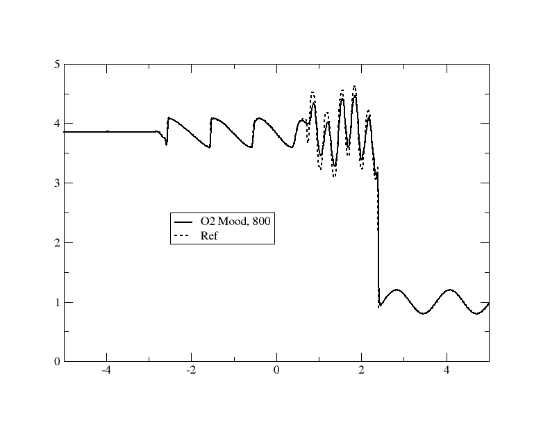
Refer to caption
(a) O2Mood
Refer to caption
(b) O4Mood
Refer to caption
(c) O2MoodNaN
Refer to caption
(d) O4MoodNaN
Figure 5: The reference solution is plotted with a dotted line. Comparison of various strategies of MOOD, for 800 points.
Refer to caption
(a) O2 800
Refer to caption
(b) O4 800
Refer to caption
(c) O2 400
Refer to caption
(d) O4 400
Refer to caption
(e) O2 200
Refer to caption
(f) O4 200
Figure 6: O2 and O4 MOOD solutions with control of NaN only, for 200, 400 and 800 mesh points.

From figure 6, we see that with 800800 points, there is hardly no difference with between the O4MoodNaN solution and the reference one.

7 Conclusion

In this paper, simplifying a method described in [16], we show how to construct a class of kinetic numerical methods that can run at least at CFL 1. They can handle in a simple manner hyperbolic problems, and in particular compressible fluid mechanics one. These methods are always locally conservative and thus can handle correctly discontinuities. We have described a rather simple stabilisation mechanism which can be further improved or changed: it is not really the core of the proposed method. Our methodology can be arbitrarily high order and can use CFL number larger or equal to unity on regular Cartesian meshes. Extension to the multidimensional case will be the topic of future works. In particular, our implementation of these methods indicates that they can be potentially very fast. The parallelisation should also be straightforward. This, however, has to be confirmed in several spatial dimensions.

Acknowledgment

R.A. would like to thanks Prof. Li-Shi Luo (Old Dominion, USA) and Professor Sagaut (Aix-Marseilles University, France) for their encouragement. Finally, he would like to thank Professors Lallemand and D’Humières for the discussion we had during his PhD studies. This paper shows that this has never been forgotten. I take this opportunity to also thanks Prof. Chi-Wang Shu for very helpfull discussions about time stepping. D.T. has been partially funded by ITN ModCompShock project funded by the European Union’s Horizon 2020 research and innovation program under the Marie Sklodowska-Curie grant agreement No 642768.

Appendix A Another iteration technique for the fourth order in time case

The iteration (2.15) solved by (2.19) reads (when we have no source term or after the application of the projector operator):

v1(p+1)=uin−λ⁡(θ01​δ​uin+θ11​δ​v1(p)+θ21​δ​v2(p))v2(p+1)=uin−λ⁡(θ02​δ​uin+θ12​δ​v1(p)+θ22​δ​v2(p))\begin{split}v_{1}^{(p+1)}=u_{i}^{n}-\lambda\big(\theta_{0}^{1}\delta u^{n}_{i}+\theta_{1}^{1}\delta v_{1}^{(p)}+\theta_{2}^{1}\delta v_{2}^{(p)}\big)\\ v_{2}^{(p+1)}=u_{i}^{n}-\lambda\big(\theta_{0}^{2}\delta u^{n}_{i}+\theta_{1}^{2}\delta v_{1}^{(p)}+\theta_{2}^{2}\delta v_{2}^{(p)}\big)\\ \end{split}

and after the application of the Fourier transform, we have

v^(p+1)=u^n​e−λ​g​θ​𝐯(p),e=(1−θ01​λ​g1−θ02​λ​g),θ=(θ11θ21θ12θ22)\hat{v}^{(p+1)}=\hat{u}^{n}e-\lambda g\theta\mathbf{v}^{(p)},\quad e=\begin{pmatrix}1-\theta_{0}^{1}\lambda g\\ 1-\theta_{0}^{2}\lambda g\end{pmatrix},\quad\theta=\begin{pmatrix}\theta_{1}^{1}&\theta_{2}^{1}\\ \theta_{1}^{2}&\theta_{2}^{2}\end{pmatrix}

so that the amplification factor satisfies

G(p+1)=e−λ​g​θ​G(p).G^{(p+1)}=e-\lambda g\theta G^{(p)}.

This can be seen as the Jacobi iteration for solving the system

(Id+λ​g​θ)​G=e.(\text{Id}+\lambda g\theta\big)G=e.

By analogy, we can define a Gauss-Seidel iteration by

v1(p+1)=uin−λ⁡(θ01​δ​uin+θ11​δ​v1(p)+θ21​δ​v2(p))v2(p+1)=uin−λ⁡(θ02​δ​uin+θ12​δ​v1(p+1)+θ22​δ​v2(p))\begin{split}v_{1}^{(p+1)}=u_{i}^{n}-\lambda\big(\theta_{0}^{1}\delta u^{n}_{i}+\theta_{1}^{1}\delta v_{1}^{(p)}+\theta_{2}^{1}\delta v_{2}^{(p)}\big)\\ v_{2}^{(p+1)}=u_{i}^{n}-\lambda\big(\theta_{0}^{2}\delta u^{n}_{i}+\theta_{1}^{2}\delta v_{1}^{(p+1)}+\theta_{2}^{2}\delta v_{2}^{(p)}\big)\\ \end{split}

whose Fourier transform is

v^(p+1)=u^n​e−λ​g​Θ1​v^(p+1)−λ​g​Θ2​v^(p),Θ1=(00θ120),Θ2=(θ11θ210θ22),\hat{v}^{(p+1)}=\hat{u}^{n}e-\lambda g\Theta_{1}\hat{v}^{(p+1)}-\lambda g\Theta_{2}\hat{v}^{(p)},\quad\Theta_{1}=\begin{pmatrix}0&0\\ \theta_{1}^{2}&0\end{pmatrix},\quad\Theta_{2}=\begin{pmatrix}\theta_{1}^{1}&\theta_{2}^{1}\\ 0&\theta_{2}^{2}\end{pmatrix},

and hence

(Id+λ​g​Θ1)​G(p+1)=e−λ​g​Θ2​G(p).(\text{Id}+\lambda g\Theta_{1})G^{(p+1)}=e-\lambda g\Theta_{2}G^{(p)}.

In both cases, G(0)=eG^{(0)}=e.

We can study the stability of the Gauss–Seidel iteration, and we recall the results of Jacobi’s for comparison. Denoting by g1g_{1} (resp. g2g_{2}, g4,1g_{4,1}, g4,2g_{4,2}) the Fourier symbol of the operators a​δ1a\delta_{1} (resp. a​δ2a\delta_{2}, a​δ41a\delta_{4}^{1}, a​δ42a\delta_{4}^{2}), we get the results of table 8.

Iterations 1 2 3 4 5
Symbol Gauss Seidel
g1g_{1} 1.5 1.2769067141.276906714 1.1672018581.167201858 1.1970671461.197067146, 1.1526289551.152628955
g2g_{2} 0 ≥1.65\geq 1.65 ≥1.47\geq 1.47 ≥1.435\geq 1.435 ≥1.55\geq 1.55
g41g_{4}^{1}22 2 always 1 for x=πx=\pi 0 ≥0.926\geq 0.926 ≥1.775\geq 1.775 0 0
g42g_{4}^{2} 0 ≥0.917\geq 0.917 0.87540139330.8754013933 ≥0.89\geq 0.89 ≥0.86\geq 0.86
Symbol Jacobi
g1g_{1} 11 11 1.2563726631.256372663 1.3926467821.392646782 1.7741611721.774161172
g2g_{2} 00 ≥0.87\geq 0.87 ≥1.625\geq 1.625 ≥1.744\geq 1.744 ≥2.06\geq 2.06
g41g_{4}^{1} 33 3 always 1 for x=πx=\pi 00 00 ≥1.25\geq 1.25 ≥2.06\geq 2.06 ≥2.52\geq 2.52
g42g_{4}^{2} 00 00 ≥0.905\geq 0.905 ≥1.044\geq 1.044 ≥1.321\geq 1.321
Table 8: CFL number for stability of the DeC iterations given by Gauss-Seidel and Jacobi methods. 00 means that the scheme is unconditionally unstable. xx means that the scheme is stable up to CFL xx, ≥x\geq x means that the scheme is stable for at least CFL x (and slightly above).
Remark A.1 (A few remarks about table 8.).

  • •

    For g41g_{4}^{1}, the amplification factor is always equal to 11 when x=πx=\pi, and strictly below 11 under the condition stated above.

  • •

    For g1g_{1} and 3 iterations, the CFL condition can be computed exactly. It is 12​4+173−12​14+173+12≈1.256372663\frac{1}{2}\sqrt[3]{4+\sqrt{17}}-\frac{1}{2}\,{\frac{1}{\sqrt[3]{4+\sqrt{17}}}}+\frac{1}{2}\approx 1.256372663.

From this results, we see that there is no fundamental reason to prefer Gauss-Seidel iteration to the Jacobi one; the coding of the Gauss-Seidel is also slightly more involved. However, this conclusion holds true only for the schemes we have considered here, and might not be true for others.

References

  • [1] S. Jin and Z. Xin. The relaxation schemes for systems of conservation laws in arbitrary space dimensions. Commun. Pure Appl. Math., 48(3):235–276, 1995.
  • [2] R. Natalini. A discrete kinetic approximation of entropy solution to multi-dimensional scalar conservation laws. Journal of differential equations, 148:292–317, 1998.
  • [3] F. Bouchut. Construction of BGK models with a family of kinetic entropies for a given system of conservation laws. Journal of Statistical Physics, 95(1/2), 1999.
  • [4] D. Aregba-Driollet and R. Natalini. Discrete kinetic schemes for multi-dimensional systems of conservation laws. SIAM J. Numer. Anal., 37(6):1971–2004, 2000.
  • [5] P. Lafitte, W. Melis, and G. Samaey. A high-order relaxation method with projective integration for solving nonlinear systems of hyperbolic conservation laws. J. Comput. Phys., 340:1–25, 2017.
  • [6] H. J. Schroll. High resolution relaxed upwind schemes in gas dynamics. In Proceedings of the Fifth International Conference on Spectral and High Order Methods (ICOSAHOM-01) (Uppsala), volume 17, pages 599–607, 2002.
  • [7] M. Banda and M. Sead. Relaxation weno schemes for multi-dimensional hyperbolic systems of conservation laws. Numer. Methods Partial Differential Equations, 23(5):1211–1234, 2007.
  • [8] D. Coulette, E. Franck, Ph. Helluy, M. Mehrenberger, and L. Navoret. High-order implicit palindromic discontinuous Galerkin method for kinetic-relaxation approximation. Computers & Fluids, 190:485 – 502, 2019.
  • [9] S. Boscarino, L. Pareschi, and G. Russo. Implicit-explicit Runge-Kutta schemes for hyperbolic systems and kinetic equations in the diffusion limit. SIAM J. Sci. Comput., 35(1):A22–A51, 2013.
  • [10] T. Xiong, G. Russo, and J.-M. Qiu. Conservative multi-dimensional semi-Lagrangian finite difference scheme: stability and applications to the kinetic and fluid simulations. J. Sci. Comput., 79(2):1241–1270, 2019.
  • [11] E. Hairer and G. Wanner. Solving ordinary differential equations. II, volume 14 of Springer Series in Computational Mathematics. Springer-Verlag, Berlin, 2010. Stiff and differential-algebraic problems, Second revised edition, paperback.
  • [12] R. J. Spiteri and S. J. Ruuth. A new class of optimal high-order strong-stability-preserving time discretization methods. SIAM J. Numer. Anal., 40(2):469–491, 2002.
  • [13] R. Abgrall. High order schemes for hyperbolic problems using globally continuous approximation and avoiding mass matrices. J. Sci. Comput., 73(2-3):461–494, 2017.
  • [14] A. Dutt, L. Greengard, and V. Rokhlin. Spectral Deferred Correction Methods for Ordinary Differential Equations. BIT Numerical Mathematics, 40(2):241–266, 2000.
  • [15] M. L. Minion. Semi-implicit spectral deferred correction methods for ordinary differential equations. Commun. Math. Sci., 1(3):471–500, 09 2003.
  • [16] R. Abgrall and D. Torlo. High order asymptotic preserving deferred correction implicit-explicit schemes for kinetic models. SIAM Journal on Scientific Computing, 42(3):B816–B845, 2020.
  • [17] F. Coron and B. Perthame. Numerical passage from kinetic to fluid equations. SIAM Journal on Numerical Analysis, 28(1):26–42, 1991.
  • [18] S. Pieraccini and G. Puppo. Implicit–explicit schemes for bgk kinetic equations. Journal of Scientific Computing, 32(1):1–28, 2007.
  • [19] A. Iserles. Order stars and saturation theorem for first-order hyperbolics. IMA J. Numer. Anal., 2:49–61, 1982.
  • [20] B. van Leer. Flux-vector splitting for the euler equations. Technical Report NAS1-151810, ICASE, 1982.
  • [21] S. Clain, S. Diot, and R. Loubère. A high-order finite volume method for systems of conservation laws – multi-dimensional optimal order detection (MOOD). Journal of Computational Physics, 230(10):4028 – 4050, 2011.
  • [22] F. Vilar. A posteriori correction of high-order discontinuous Galerkin scheme through subcell finite volume formulation and flux reconstruction. Journal of Computational Physics, 387:245 – 279, 2019.
  • [23] D. Kuzmin. A vertex-based hierarchical slope limiter for pp-adaptive discontinuous Galerkin methods. Journal of Computational and Applied Mathematics, 233(12):3077–3085, 2010.