Deep Fitting Degree Scoring Network for Monocular 3D Object Detection
Abstract
In this paper, we propose to learn a deep fitting degree scoring network for monocular 3D object detection, which aims to score fitting degree between proposals and object conclusively. Different from most existing monocular frameworks which use tight constraint to get 3D location, our approach achieves high-precision localization through measuring the visual fitting degree between the projected 3D proposals and the object. We first regress the dimension and orientation of the object using an anchor-based method so that a suitable 3D proposal can be constructed. We propose FQNet, which can infer the 3D IoU between the 3D proposals and the object solely based on 2D cues. Therefore, during the detection process, we sample a large number of candidates in the 3D space and project these 3D bounding boxes on 2D image individually. The best candidate can be picked out by simply exploring the spatial overlap between proposals and the object, in the form of the output 3D IoU score of FQNet. Experiments on the KITTI dataset demonstrate the effectiveness of our framework.
1 Introduction
2D perception is far from the requirements for people’s daily use as people live in a 3D world essentially. In many applications such as autonomous driving bertozzi2000vision; chen2015deepdriving; janai2017computer; bai2018group; duan2018ai and vision-based grasping saxena2008robotic; mahler2017dex; levine2018learning, we usually need to reason about the 3D spatial overlap between objects in order to understand the realistic scene and take further action. 3D object detection is one of the most important problems in 3D perception, which requires solving a 9 Degree of Freedom (DoF) problem including dimension, orientation, and location. Although great progress has been made in stereo-based leibe2007dynamic; chen20153d; chen20183d, RGBD-based lin2013holistic; song2014sliding; gupta2015aligning; song2016deep; qi2017frustum and point-cloud-based wang2015voting; li2016vehicle; engelcke2017vote3deep; chen2017multi; li20173d; ku2017joint; asvadi2017depthcn; beltran2018birdnet; zeng2018rt3d 3D object detection methods, monocular-image-based approaches have not been thoroughly studied yet, and most of existing works focus on the sub-problem, such as orientation estimation chen2016monocular; xiang2017subcategory; mousavian20173d. The primary cause is that under monocular setting, the only cue is the appearance information in the 2D image, and the real 3D information is not available, which makes the problem ill-conditioned. However, in many cases, such as web images, mobile applications duan2016overview, and gastroscopy, the information of depth or point-cloud is not available or unaffordable. Moreover, in some extreme scenarios, other sensors can be broken. Therefore, considering the rich source of monocular images and the robustness requirements of the system, monocular 3D object detection problem is of crucial importance.

In monocular 3D object detection problem, dimension and orientation estimation are easier than location estimation, because the only available information, appearance, is strongly related to the former two sub-problems. On the contrary, it is not practical to directly regress location using a single image patch, since nearby and faraway objects with same pose are substantially identical in appearance.
Tight constraint mousavian20173d; kundu20183d is a commonly used method in monocular 3D object detection problem, which solves the location by placing the 3D proposal in the 2D bounding box compactly. However, the tight constraint has two significant drawbacks: 1) Image appearance cue is not used; thus it cannot benefit from a large number of labeled data in the training set. 2) Its performance highly depends on the 2D detection accuracy, as shown in Figure 1.
Inspired by the observation that people can easily distinguish the quality of 3D detection results through projecting these 3D bounding boxes on the 2D image and checking the relation between projections and object (fitting degree), we believe that exploring the 3D spatial overlap between proposals and ground-truth is the key to solve the location estimation problem. In this paper, we first regress the dimension and orientation of the object using an anchor-based method so that we can construct a suitable 3D proposal. The reason why we emphasize the importance of the regression step is that without an appropriate proposal, checking the fitting degree is impractical. Then, we propose Fitting Quality Network (FQNet) to infer 3D Intersection over Union (IoU) between 3D proposals and object only using 2D information. Our motivation is that though the 3D location is independent of 2D appearance, drawing the projection results on the 2D image can bring additional information for the convolutional neural network (CNN) to better understand the spatial relationship between the original 3D bounding boxes and the object. As long as the network learns the pattern of the projected 3D bounding boxes, it can gain the power of judging the relation between 3D proposals and the object, and achieve high-precision 3D perception. Figure 1 gives an illustration of the essential difference between our idea and existing tight constraint-based method. We can see that our method is not sensitive to the error of 2D detection results. To the best of our knowledge, we are the first to solve the monocular 3D detection problem by exploring the fitting degree between 3D proposals and object. We conducted experiments on the challenging KITTI dataset and achieved state-of-the-art monocular 3D object detection performance, which demonstrates the effectiveness of our framework.
2 Related Work
Monocular 3D Object Detection: Monocular 3D object detection is much more difficult than 2D object detection because of the ambiguities arising from 2D-3D mapping. Many methods have taken the first step, which can roughly categorize into two classes: handcrafted approaches and deep learning based approaches.
Most of the early works belong to the handcrafted approaches, which concentrated on designing efficient handcrafted features. Payet and Todorovic payet2011contours used image contours as basic features and proposed mid-level features, called bags of boundaries (BOBs). Fidler et al. fidler20123d extended the Deformable Part Model (DPM) and represented an object class as a deformable 3D cuboid composed of faces and parts. Pepik et al. pepik2015multi included viewpoint information and part-level 3D geometry information in the DPM and achieved robust 3D object representation. Although these handcrafted methods are very carefully designed and perform well on some scenarios, their generalization ability is still limited.
Deep learning based approaches aim to benefit from end-to-end training and a large amount of labeled data. Chen et al. chen2016monocular generated a set of candidate class-specific object proposals on a ground prior and used a standard CNN pipeline to obtain high-quality object detections. Mousavian et al. mousavian20173d presented MultiBin architecture for orientation regression and tight constraint to solve the 3D translation. Kundu et al. kundu20183d trained a deep CNN to map image regions to the full 3D shape and pose of all object instances in the image. Apart from these pure monocular methods, there are some other methods which use additional information for training. Xu and Chen xu2018multi proposed to fuse a monocular depth estimation module and achieved high-precision localization. Chabot et al. chabot2017deep presented Deep MANTA (Deep Many-Tasks) for simultaneous vehicle detection, part localization and visibility characterization, but their method requires part locations and visibility annotations.
In this paper, we propose a unified deep learning based pipeline, which does not require additional labels and can be trained end-to-end using a large number of augmented data.
Box Refinement Techniques: Our work has some similarities to the box refinement techniques, which focused on improving the localization accuracy. In 2D object detection, the most common method is the bounding box regression, which was first proposed by Felzenszwalb et al. felzenszwalb2010object and has been used in many state-of-the-art detectors, such as Faster R-CNN ren2015faster and SPP-net he2015spatial. Gidaris and Komodakis gidaris2016locnet proposed LocNet to further improve the object-specific localization accuracy through assigning probabilities to the boundaries. While in monocular 3D object detection, the work on this level has been limited. Xiao et al. xiao2012localizing proposed to localize the corners using a discriminative parts-based detector. Many works also used stronger representations to achieve high-precision localization. For example, Zia et al. zia2015towards used a fine-grained 3D shape model, Xiang and Savarese xiang2013object introduced 3D aspectlet based on a piecewise planar object representation and Pero et al. del2013understanding proposed to use detailed geometric models. In our case, we stick to the 3D bounding box representation and learn the pattern of projected boxes on the 2D image.
3 Approach
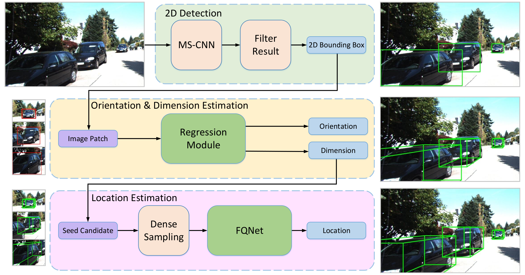
Our framework only requires a single image as input and can output precise 3D detection results including dimension, orientation, and location of interested objects. Figure 2 shows the overall pipeline, where we first perform regular 2D detection11 1 We use a popular 2D detection algorithm cai2016unified to produce the 2D detection results. and then use an anchor-based regression module to regress the dimension and orientation of each object based on the image patch cropped by 2D detection results. For the 3D location, we first use tight constraint to get a seed-candidate, then perform Gaussian dense sampling to generate a large number of candidates within a small range around the seed-candidate. To evaluate these candidates, we train a Fitting Quality Network (FQNet) to infer the 3D IoU between a large number of augmented samples and the ground truth. Therefore, by estimating the fitting degree between the candidates and the object, the candidate with the highest score will be chosen as the 3D detection result. Our framework separates the dimension and orientation estimation process from the location estimation because we consider that these tasks are fundamentally different (orientation and dimension are all appearance-related but the location is not) and the results of dimension and orientation regression have a significant impact on the location estimation process.
3.1 Regression Module
The input of our regression module is the cropped detection result of 2D object detection, while the output is the dimension and orientation of each object.
For dimension, based on appearance, it is not difficult to infer the type of cars, and cars of the same type usually have similar length, width, and height. For orientation, it is a bit more complicated since there are global orientation and local orientation, but intuitively we can be sure that different orientation will show different appearance.
Dimension Estimation: To regress the dimension as accurate as possible, we propose an idea called anchor cuboid, whose philosophy is similar to MultiBin mousavian20173d. We first perform k-means clustering on the training dataset to find the cluster centers of the dimension and regard these cluster centers as 3D anchor cuboids. During the regression process, the regression module outputs confidence and offset for each 3D anchor cuboid respectively, so the output is a -dimensional vector (), and the final regression result is the anchor cuboid with the highest confidence adding corresponding offsets. We optimize this module using the following loss function:
| (1) |
where the 22 2 It is worth mentioning that the value of for each object can be computed and saved in the dataset before the training process. means among anchor cuboid, the -th anchor cuboid has the maximum IoU with the ground-truth cuboid , and are the offsets in three different dimensions relative to anchor cuboid . The is the softmax function:
| (2) |
and the function computes the 3D IoU between two center-aligned cuboids:
| (3) |
There are two terms in the Equation (1). For the first term, it encourages the module to give the highest confidence to the anchor cuboid which has the maximum IoU with the ground truth dimension , and provides low confidence for other anchor cuboids at the same time. For the second term, it encourages the module to regress the offset between the best anchor cuboid and ground truth cuboid. Our loss function is volume-driven rather than dimension-driven, and the rationale is that it can take into account the information from three dimensions synthetically and avoid the situation that two dimensions have good estimation while one dimension is not well estimated.
Orientation Estimation: There are two orientations in the 3D object detection problem, global orientation and local orientation. The global orientation of an object is defined under the world coordinates and will not change with the camera pose, while the local orientation is defined under the camera coordinates and hinges on how the camera shots the object. Figure 3 gives an illustration of these two kinds of orientation from the bird’s view. In this paper, we focus on the estimation of the local orientation, which is evaluated in the KITTI dataset and directly related to the appearance.


For orientation regression, the range of the output is , we use a similar idea to dimension regression and perform k-means clustering on the training set to get cluster centers. The output is a -dimensional vector (). We define the loss function as follows:
| (4) |
where is the nearest anchor angle comparing to the ground truth local orientation . The first term in the loss function is the same as which encourages the module to give high confidence to the nearest anchor angle, and the second term uses the cosine function to ensure that the offset can be well regressed.
The idea behind our anchor-based regression is that directly regress a continuous variable is very difficult because the value range is vast. Using an anchor-based method, we can first solve a classification problem to choose the best anchor, and then regress an offset based on the anchor value; hence the value range that we need to regress can be significantly reduced. We show the concrete architecture of our proposed regression module in Figure 4.
3.2 Location Estimation
After estimating the dimension and orientation, we can construct a 3D cuboid in 3D spatial space. We set the original coordinate of 8 vertices of the cuboid as:
| (5) |
where are the dimensions of the object. Assume that the 3D location is in the camera coordinate, according to the law of camera projection, we have
| (6) |
where and are the 2D projected coordinates of the -th vertices, is the intrinsic matrix, and is the rotation matrix given by the global orientation :
| (7) |
We can use OpenCV toolkit to draw the projected 3D bounding box on the 2D image based on the 2D projected coordinates; thus, our FQNet can learn from these 2D projection patterns and obtain the ability to reason 3D spatial relations.
Dense Sampling: We use a sampling and evaluation framework. Sampling in the whole 3D space is time-consuming, so we choose to get an approximate location (seed candidate) first. Many methods can achieve this goal, such as performing uniform sampling and searching the proposal whose 2D projection has the largest overlap with the 2D detection result. Here, we choose to use tight constraint similar in mousavian20173d; kundu20183d to locate the seed candidate, because it is fast and relatively more accurate. After computing the location of seed-candidate, we can perform dense sampling within a small range around it. We model the distribution of the transition value in three axes as three independent Gaussian distribution as follows:
| (8) |
where the mean and variance are all estimated using the 3D localization error in the training set. Thus, the -th generated sample can be represented as .
FQNet: The goal of FQNet is to evaluate the fitting quality between each sample and object. Even though it is challenging for CNN to infer the spatial relation between and ground-truth 3D location of the object, after projecting the sample on the 2D image, CNN can obtain this ability through learning the pattern that how well the edges and corners of projections are aligned with the specific part of the object. For quantitative analysis, we force the network to regress the 3D IoU between samples and the object. Denote the object image patch as , the objective of FQNet can be formulated as follows:
| (9) |
where denotes the parameters of FQNet.
Since we have the ground-truth 3D location of each object in our training set, we can generate an almost unlimited number of samples by adding a known jitter to the original 3D location. One problem is that how can we guarantee that FQNet can capture the pattern of the projection, which we painted on the 2D image manually. To answer this question, we first pre-train our FQNet to execute a classification task, in which it has to decide whether the input image patch contains an artificially painted 3D bounding box projection or not. The architecture of our proposed FQNet and its pre-training version are shown in Figure 5. For the pre-training process, we use the cross-entropy loss for the classification task. For the 3D IoU regression, we use the smooth L1 loss, since it is less sensitive to outliers compared to the L2 loss.
4 Experiments
We evaluated our method on the real-world KITTI dataset geiger2012we. The KITTI object detection benchmark includes 2D Object Detection Evaluation, 3D Object Detection Evaluation and Bird’s Eye View Evaluation. There are 7481 training images and 7518 testing images in the dataset, and in each image, the object is annotated with observation angle (local orientation), 2D location, dimension, 3D location, and global orientation. However, only the labels in the KITTI training set are released, so we mainly conducted controlled experiments in the training set. Results are evaluated based on three levels of difficulty: Easy, Moderate, and Hard, which is defined according to the minimum bounding box height, occlusion and truncation grade. There are two commonly used train/val experimental settings: Chen et al. chen20153d; chen2016monocular (train/val 1) and Xiang et al. xiang2015data; xiang2017subcategory (train/val 2). Both splits guarantee that images from the training set and validation set are from different videos. We focused our experiment on the Car object category since, for Pedestrian and Cyclist, there is not enough data to train our model.
4.1 Implementation Details
For regression module, we used the ImageNet deng2009imagenet pre-trained VGG-16 simonyan2014very model with input size to initialize the weights of convolutional layers. We used four anchor cuboids during dimension estimation and two anchor angles during orientation estimation. The module is trained with SGD using a fixed learning rate of with a batch size of 8. We performed data augmentation by adding color distortions, flipping images at random, and jittering 2D boxes with a translation of x height and width.
For dense sampling process, we first sampled 1024 samples around the seed candidate. After discarding the samples more than half of which are outside the image plane, we kept 640 samples for evaluation.
| Method | Easy | Moderate | Hard | ||||||
|---|---|---|---|---|---|---|---|---|---|
| train/val 1 | train/val 2 | test | train/val 1 | train/val 2 | test | train/val 1 | train/val 2 | test | |
| 3DOP chen20153d | 91.58 | - | 91.44 | 85.80 | - | 86.10 | 76.80 | - | 76.52 |
| Mono3D chen2016monocular | 91.90 | - | 91.01 | 86.28 | - | 86.62 | 77.09 | - | 76.84 |
| 3DVP xiang2015data | - | 78.99 | 86.92 | - | 65.73 | 74.59 | - | 54.67 | 64.11 |
| SubCNN xiang2017subcategory | - | 94.55 | 90.67 | - | 85.03 | 88.62 | - | 72.21 | 78.68 |
| Deep3DBox mousavian20173d | - | 97.50 | 92.90 | - | 96.30 | 88.75 | - | 80.40 | 76.76 |
| 3D-RCNN kundu20183d | 90.70 | 97.70 | 89.98 | 89.10 | 96.50 | 89.25 | 79.50 | 80.70 | 80.07 |
| Our Method | 97.28 | 97.57 | 92.58 | 93.70 | 96.70 | 88.72 | 79.25 | 80.45 | 76.85 |
| Method | IoU = 0.5 | IoU = 0.7 | ||||||||||
|---|---|---|---|---|---|---|---|---|---|---|---|---|
| Easy | Moderate | Hard | Easy | Moderate | Hard | |||||||
| t/v 1 | t/v 2 | t/v 1 | t/v 2 | t/v 1 | t/v 2 | t/v 1 | t/v 2 | t/v 1 | t/v 2 | t/v 1 | t/v 2 | |
| 3DOP chen20153d | 55.04 | - | 41.25 | - | 34.55 | - | 12.63 | - | 9.49 | - | 7.59 | - |
| Mono3D chen2016monocular | 30.50 | - | 22.39 | - | 19.16 | - | 5.22 | - | 5.19 | - | 4.13 | - |
| Deep3DBox mousavian20173d | - | 30.02 | - | 23.77 | - | 18.83 | - | 9.99 | - | 7.71 | - | 5.30 |
| Our Method | 32.57 | 33.37 | 24.60 | 26.29 | 21.25 | 21.57 | 9.50 | 10.45 | 8.02 | 8.59 | 7.71 | 7.43 |
| Method | train/val 1 | train/val 2 |
|---|---|---|
| 3DOP chen20153d | 0.3527 | - |
| Mono3D chen2016monocular | 0.4251 | - |
| Deep3DBox mousavian20173d | - | 0.1934 |
| Our Method | 0.1698 | 0.1465 |
For FQNet, we used the ImageNet pre-trained VGG-M model with input size to initialize the weights of convolutional layers. The projection was drawn using green color and linewidth of 1. For the classification pre-training process, we sampled 256 positive samples and 256 negative samples to train the network for each iteration with learning rates for convolutional layers and for fully connected layers. For the 3D IoU regression, we mapped the labels from to for data balance. We also added a random contour context information to the training image patch to increase the robustness of the model.
4.2 Effectiveness
To demonstrate that our proposed pipeline is not sensitive to the 2D detection results, we performed jitter to the MS-CNN 2D detection results and got a set of 2D bounding boxes with different Average Precision (AP). We compared the 3D detection performance (3D AP) of our method with the tight-constraint-based baseline, and the results are shown in Figure 6. We can see that the tight-constraint-based method is much more sensitive to the 2D detection AP, while our approach is much more robust.
We also studied our FQNet module by evaluating the 3D IoU regression performance. After dividing all proposals into ten levels based on the 3D IoU, we computed the average regression error for each level and drew the histogram in Figure 7. We can see that for the samples whose 3D IoU is around 0.4 to 0.5, the average estimation error is the lowest, which is about 0.05. Therefore, we can be sure that our FQNet have the ability to evaluate candidates.
| Method | IoU = 0.5 | IoU = 0.7 | ||||||||||
|---|---|---|---|---|---|---|---|---|---|---|---|---|
| Easy | Moderate | Hard | Easy | Moderate | Hard | |||||||
| t/v 1 | t/v 2 | t/v 1 | t/v 2 | t/v 1 | t/v 2 | t/v 1 | t/v 2 | t/v 1 | t/v 2 | t/v 1 | t/v 2 | |
| 3DOP chen20153d | 46.04 | - | 34.63 | - | 30.09 | - | 6.55 | - | 5.07 | - | 4.10 | - |
| Mono3D chen2016monocular | 25.19 | - | 18.20 | - | 15.52 | - | 2.53 | - | 2.31 | - | 2.31 | - |
| Deep3DBox mousavian20173d | - | 27.04 | - | 20.55 | - | 15.88 | - | 5.85 | - | 4.10 | - | 3.84 |
| Our Method | 28.16 | 28.98 | 21.02 | 20.71 | 19.91 | 18.59 | 5.98 | 5.45 | 5.50 | 5.11 | 4.75 | 4.45 |

4.3 Comparison with State-of-the-Arts
We compared our proposed method with 6 recently proposed state-of-the-art 3D object detection methods on the KITTI benchmark, including 3DOP chen20153d, Mono3D chen2016monocular, 3DVP xiang2015data, SubCNN xiang2017subcategory, Deep3DBox mousavian20173d and 3D-RCNN kundu20183d. For fair comparisons, we used the detection results reported by the authors. All experiments were conducted on both two validation splits (different models are trained with the corresponding training sets).
Orientation and Dimension Evaluation: For orientation evaluation, we used the official metric of the KITTI dataset, which is the Average Orientation Similarity (AOS).
Our results are summarized in Table 1. From the results, we see that our method achieves state-of-the-art method on both train/val 1 and train/val 2 experimental settings. And we can see that especially for the train/val 1 on Easy and Moderate setting, our method has a significant improvement comparing with existing methods.
For dimension evaluation, we use the average error defined as:
| (10) |
Since the detection results and the ground truth are not one-to-one equivalents, we have to find the corresponding object in the ground truth which is closest to the detection result for computing . Not all methods provided their experimental results, so we only compare our method with 3DOP chen20153d, Mono3D chen2016monocular, and Deep3DBox mousavian20173d.
Our results are summarized in Table 3. We can see that our methods have the lowest estimation error with an average dimension estimation error of about 0.15 meters, which demonstrate the effectiveness of our anchor based regression module.
Location Evaluation:
For location evaluation, we first reported our results on the official evaluation metrics from KITTI Bird’s Eye View Evaluation, where AP for the bird’s eye view boxes is evaluated, which are obtained by projecting the 3D boxes to the ground plane and neglect the location precision on the Y-axis. From Table 2, we can see that our method outperformed Mono3D chen2016monocular and Deep3DBox mousavian20173d by a significant margin of about 3% improvement. Since 3DOP chen20153d is a stereo-based method that can obtain depth information directly, so its performance is much better than pure monocular based methods.
We also conducted experiments on 3D Object Detection Evaluation, where the 3D AP metric is used to evaluate the full 3D bounding boxes. From Table 4, we can see that our method ranks first among pure monocular based methods, and we even outperformed stereo-based 3DOP when 3D IoU threshold is set to 0.7.
4.4 Qualitative Results
Apart from drawing the 3D detection boxes on 2D images, we also projected the 3D detection boxes in the 3D space for better visualization. As shown in Figure 8, our approach can fit the object well and achieve high-precision 3D perception in various scenes with only one monocular image as input.
5 Conclusions
In this paper, we have proposed a unified pipeline for monocular 3D object detection. By using an anchor-based regression method, we achieved a high-precision dimension and orientation estimation. Then we perform dense sampling in the 3D space and project these samples on a 2D image. Through measuring the relation between the projections and object, our FQNet successfully estimates the 3D IoU and filters the suitable candidate. Both quantitative and qualitative results have demonstrated that our proposed method outperforms the state-of-the-art monocular 3D object detection methods. How to extend our monocular 3D object detection method for monocular 3D object tracking seems to be interesting future work.
Acknowledgement
This work was supported in part by the National Natural Science Foundation of China under Grant 61822603, Grant U1813218, Grant U1713214, Grant 61672306, and Grant 61572271.
References
- (1) A. Asvadi, L. Garrote, C. Premebida, P. Peixoto, and U. J. Nunes. Depthcn: Vehicle detection using 3d-lidar and convnet. In ITSC, 2017.
- (2) Y. Bai, Y. Lou, F. Gao, S. Wang, Y. Wu, and L.-Y. Duan. Group-sensitive triplet embedding for vehicle reidentification. TMM, 20(9):2385–2399, 2018.
- (3) J. Beltran, C. Guindel, F. M. Moreno, D. Cruzado, F. Garcia, and A. de la Escalera. Birdnet: a 3d object detection framework from lidar information. arXiv preprint arXiv:1805.01195, 2018.
- (4) M. Bertozzi, A. Broggi, and A. Fascioli. Vision-based intelligent vehicles: State of the art and perspectives. Robotics and Autonomous systems, 32(1):1–16, 2000.
- (5) Z. Cai, Q. Fan, R. S. Feris, and N. Vasconcelos. A unified multi-scale deep convolutional neural network for fast object detection. In ECCV, 2016.
- (6) F. Chabot, M. Chaouch, J. Rabarisoa, C. Teulière, and T. Chateau. Deep manta: A coarse-to-fine many-task network for joint 2d and 3d vehicle analysis from monocular image. In CVPR, 2017.
- (7) C. Chen, A. Seff, A. Kornhauser, and J. Xiao. Deepdriving: Learning affordance for direct perception in autonomous driving. In ICCV, 2015.
- (8) X. Chen, K. Kundu, Z. Zhang, H. Ma, S. Fidler, and R. Urtasun. Monocular 3d object detection for autonomous driving. In CVPR, 2016.
- (9) X. Chen, K. Kundu, Y. Zhu, A. G. Berneshawi, H. Ma, S. Fidler, and R. Urtasun. 3d object proposals for accurate object class detection. In NIPS, 2015.
- (10) X. Chen, K. Kundu, Y. Zhu, H. Ma, S. Fidler, and R. Urtasun. 3d object proposals using stereo imagery for accurate object class detection. TPAMI, 40(5):1259–1272, 2018.
- (11) X. Chen, H. Ma, J. Wan, B. Li, and T. Xia. Multi-view 3d object detection network for autonomous driving. In CVPR, 2017.
- (12) L. Del Pero, J. Bowdish, B. Kermgard, E. Hartley, and K. Barnard. Understanding bayesian rooms using composite 3d object models. In CVPR, pages 153–160, 2013.
- (13) J. Deng, W. Dong, R. Socher, L.-J. Li, K. Li, and L. Fei-Fei. Imagenet: A large-scale hierarchical image database. In CVPR, 2009.
- (14) L. Duan, Y. Lou, S. Wang, W. Gao, and Y. Rui. Ai oriented large-scale video management for smart city: Technologies, standards and beyond. IEEE MultiMedia, 2018.
- (15) L.-Y. Duan, V. Chandrasekhar, J. Chen, J. Lin, Z. Wang, T. Huang, B. Girod, and W. Gao. Overview of the mpeg-cdvs standard. TIP, 25(1):179–194, 2016.
- (16) M. Engelcke, D. Rao, D. Z. Wang, C. H. Tong, and I. Posner. Vote3deep: Fast object detection in 3d point clouds using efficient convolutional neural networks. In ICRA, 2017.
- (17) P. F. Felzenszwalb, R. B. Girshick, D. McAllester, and D. Ramanan. Object detection with discriminatively trained part-based models. TPAMI, 32(9):1627–1645, 2010.
- (18) S. Fidler, S. Dickinson, and R. Urtasun. 3d object detection and viewpoint estimation with a deformable 3d cuboid model. In NIPS, 2012.
- (19) A. Geiger, P. Lenz, and R. Urtasun. Are we ready for autonomous driving? the kitti vision benchmark suite. In CVPR, 2012.
- (20) S. Gidaris and N. Komodakis. Locnet: Improving localization accuracy for object detection. In CVPR, pages 789–798, 2016.
- (21) S. Gupta, P. Arbeláez, R. Girshick, and J. Malik. Aligning 3d models to rgb-d images of cluttered scenes. In CVPR, 2015.
- (22) K. He, X. Zhang, S. Ren, and J. Sun. Spatial pyramid pooling in deep convolutional networks for visual recognition. TPAMI, 37(9):1904–1916, 2015.
- (23) J. Janai, F. Güney, A. Behl, and A. Geiger. Computer vision for autonomous vehicles: Problems, datasets and state-of-the-art. arXiv preprint arXiv:1704.05519, 2017.
- (24) J. Ku, M. Mozifian, J. Lee, A. Harakeh, and S. Waslander. Joint 3d proposal generation and object detection from view aggregation. arXiv preprint arXiv:1712.02294, 2017.
- (25) A. Kundu, Y. Li, and J. M. Rehg. 3d-rcnn: Instance-level 3d object reconstruction via render-and-compare. In CVPR, 2018.
- (26) B. Leibe, N. Cornelis, K. Cornelis, and L. Van Gool. Dynamic 3d scene analysis from a moving vehicle. In CVPR, 2007.
- (27) S. Levine, P. Pastor, A. Krizhevsky, J. Ibarz, and D. Quillen. Learning hand-eye coordination for robotic grasping with deep learning and large-scale data collection. IJRR, 37(4-5):421–436, 2018.
- (28) B. Li. 3d fully convolutional network for vehicle detection in point cloud. In IROS, 2017.
- (29) B. Li, T. Zhang, and T. Xia. Vehicle detection from 3d lidar using fully convolutional network. arXiv preprint arXiv:1608.07916, 2016.
- (30) D. Lin, S. Fidler, and R. Urtasun. Holistic scene understanding for 3d object detection with rgbd cameras. In ICCV, 2013.
- (31) J. Mahler, J. Liang, S. Niyaz, M. Laskey, R. Doan, X. Liu, J. A. Ojea, and K. Goldberg. Dex-net 2.0: Deep learning to plan robust grasps with synthetic point clouds and analytic grasp metrics. arXiv preprint arXiv:1703.09312, 2017.
- (32) A. Mousavian, D. Anguelov, J. Flynn, and J. Košecká. 3d bounding box estimation using deep learning and geometry. In CVPR, 2017.
- (33) N. Payet and S. Todorovic. From contours to 3d object detection and pose estimation. In ICCV, 2011.
- (34) B. Pepik, M. Stark, P. Gehler, and B. Schiele. Multi-view and 3d deformable part models. TPAMI, 37(11):2232–2245, 2015.
- (35) C. R. Qi, W. Liu, C. Wu, H. Su, and L. J. Guibas. Frustum pointnets for 3d object detection from rgb-d data. arXiv preprint arXiv:1711.08488, 2017.
- (36) S. Ren, K. He, R. Girshick, and J. Sun. Faster r-cnn: Towards real-time object detection with region proposal networks. In NIPS, pages 91–99, 2015.
- (37) A. Saxena, J. Driemeyer, and A. Y. Ng. Robotic grasping of novel objects using vision. IJRR, 27(2):157–173, 2008.
- (38) K. Simonyan and A. Zisserman. Very deep convolutional networks for large-scale image recognition. arXiv preprint arXiv:1409.1556, 2014.
- (39) S. Song and J. Xiao. Sliding shapes for 3d object detection in depth images. In ECCV, 2014.
- (40) S. Song and J. Xiao. Deep sliding shapes for amodal 3d object detection in rgb-d images. In CVPR, 2016.
- (41) D. Z. Wang and I. Posner. Voting for voting in online point cloud object detection. In Robotics: Science and Systems, volume 1, 2015.
- (42) Y. Xiang, W. Choi, Y. Lin, and S. Savarese. Data-driven 3d voxel patterns for object category recognition. In CVPR, 2015.
- (43) Y. Xiang, W. Choi, Y. Lin, and S. Savarese. Subcategory-aware convolutional neural networks for object proposals and detection. In WACV, 2017.
- (44) Y. Xiang and S. Savarese. Object detection by 3d aspectlets and occlusion reasoning. In ICCVW, pages 530–537, 2013.
- (45) J. Xiao, B. Russell, and A. Torralba. Localizing 3d cuboids in single-view images. In Advances in neural information processing systems, pages 746–754, 2012.
- (46) B. Xu and Z. Chen. Multi-level fusion based 3d object detection from monocular images. In CVPR, 2018.
- (47) Y. Zeng, Y. Hu, S. Liu, J. Ye, Y. Han, X. Li, and N. Sun. Rt3d: Real-time 3-d vehicle detection in lidar point cloud for autonomous driving. IEEE Robotics and Automation Letters, 3(4):3434–3440, 2018.
- (48) M. Z. Zia, M. Stark, and K. Schindler. Towards scene understanding with detailed 3d object representations. IJCV, 112(2):188–203, 2015.