A Block Sparsity Based Estimator for mmWave Massive MIMO Channels with Beam Squint

We consider a mmWave massive MIMO system, focusing on the uplink transmission. The BS is equipped with a uniform linear array (ULA) consisting of $M$ antennas, where $M$ is a large integer, and the antenna spacing is $d=\lambda_{c}^{\text{ul}}/2$. Here, $\lambda_{c}^{\text{ul}}\triangleq{c}/{f_{c}^{\text{ul}}}$, where $f_{c}^{\text{ul}}$ is the uplink center frequency, $\lambda_{c}^{\text{ul}}$ is the wavelength, and $c$ is the speed of light. To present the channel model, highlighting the spatial wideband effect, we discuss the case of a single user with a single antenna and assume a noiseless setup in this subsection. The proposed model can be extended to multiple users with multiple antennas by properly adapting the arguments in the sequel.

To formulate the channel model, we use $\alpha[i]$ to denote the discrete-time baseband transmitted symbol, with symbol period $T_{s}$. The continuous-time baseband transmit signal $\bar{s}(t)$ can thus be expressed as

where $g(t)$ is the pulse shaping function. After modulating, the passband transmit signal $\tilde{s}(t)$ can be written as

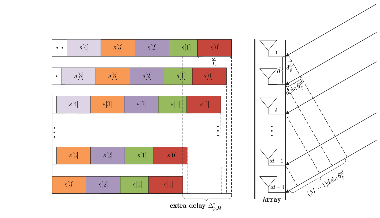
Let $P$ denote the number of paths between the user and the BS. Each path has direction of arrival (DOA) $\theta_{p}^{\text{ul}}\in[-\pi/2,\pi/2)$ and passband gain $\beta_{p}^{\text{ul}}\in\mathbb{R}^{+}$. Denote the $p$th path delay between the transmitter and the first receive antenna by $\tau_{p}^{\text{ul}}$. Unlike conventional MIMO models, the large array aperture of massive MIMO receivers results in non-negligible delays among different antennas. Those delays are present even for received signal components corresponding to the same channel path, as illustrated in Fig. 1. The extra delay of the $p$th path from the $m$th receive antenna compared to the first receive antenna is given by

Consequently, the passband receive signal at the $m$th antenna can be written as

For conventional MIMO systems, where $M$ is small or the bandwidth is narrow, it typically holds that $\Delta^{\tau}_{p,m}\ll T_{s}$ for each $m\in\{0,1,\ldots,M-1\}$. Thus the signals at different antennas satisfy $\bar{s}(t-\tau_{p}^{\text{ul}}-\Delta^{\tau}_{p,m})\approx\bar{s}(t-\tau_{p}^{\text{ul}})$. Namely, different antennas at the BS effectively observe a synchronized signal. In such scenarios, the standard MIMO channel output model, i.e., a linear convolution between the individual channel impulse responses and the same source signal, faithfully represents the received signal.

However, for mmWave massive MIMO systems, $\Delta^{\tau}_{p,m}$ cannot be ignored for larger values of $m$, and the approximation $\bar{s}(t-\tau_{p}^{\text{ul}}-\Delta^{\tau}_{p,m})\approx\bar{s}(t-\tau_{p}^{\text{ul}})$ no longer holds. In this case, the signal observed by the first antenna will include a different time shift compared to the signals observed by other antennas. This phenomenon is referred to as the spatial wideband effect [20]. As an illustrative example, consider a massive MIMO system with $M=128$ BS antennas, $\theta^{\text{ul}}_{p}=60^{\circ}$, baseband symbol rate $f_{s}=\frac{1}{T_{s}}=2$GHz, and mmWave carrier frequency $f_{c}^{\text{ul}}=60$GHz. Under this setting, the signal delay between the first antenna and the last one, computed via (3), is $1.85T_{s}$, which is clearly non-negligible.

In the presence of the spatial wideband effect, it is difficult to formulate a unified discrete-time MIMO channel model since the signals arrive at different antennas with relative delays which are fractions of the symbol period. To derive a convenient model which facilitates analysis, we observe the transmission in an antenna-by-antenna manner. From (II-A), removing the center frequency $f_{c}^{\text{ul}}$, to switch from passband to baseband representation, the continuous-time baseband receive signal at the $m$th antenna is given by

where $\bar{\beta}_{p}^{\text{ul}}\triangleq\beta_{p}^{\text{ul}}e^{-j2\pi f_{c}^{\text{ul}}\tau_{p}^{\text{ul}}}$ is the equivalent complex channel gain, and $*$ denotes the convolution operator. Taking the Fourier transform of (II-A), we obtain the frequency-domain representation of the received signal at the $m$th antenna as:

where $\phi_{p}^{\text{ul}}\triangleq\frac{2\pi d\cdot\sin(\theta_{p}^{\text{ul}})}{\lambda_{c}^{\text{ul}}}\in[-\pi,\pi)$ is defined as the normalized DOA. For clarity, in the rest of the paper, the term “DOA” will refer to the normalized DOA.

By stacking the received signal $y_{m}^{\text{ul}}(f)$ over all $M$ antennas into a single vector representation, we can write

where

is the uplink channel frequency response, and

is the wideband array steering vector. Note that unlike conventional array steering vectors, see, e.g., [16, 17, 18], the wideband array steering vector $\bm{a}(\phi_{p}^{\text{ul}},f)$ is frequency-dependent.

We next focus on OFDM signaling with $N$ subcarriers and subcarrier spacing $f_{0}$. We henceforth assume that the number of antennas $M$ satisfies $M\leq 2N\frac{f_{c}^{\rm up}}{f_{s}}$. This assumption is reasonable for mmWave systems in which the bandwidth is very large, thus the number of subcarriers $N$ is of the same order as $M$, and the carrier frequency $f_{c}^{\rm up}$ is much larger than the symbol rate $f_{s}$.

Using (8), the uplink channel vector corresponding to the $n$th subcarrier can be written as

for each $n=\{0,1,\ldots,N-1\}$, where $\bm{W}(\phi_{p}^{\text{ul}})$ is the $M\times N$ matrix of wideband factors whose $(m,n)$th entry is given by

The overall $M\times N$ uplink channel matrix for the OFDM system can then be written as

In previous works, e.g., [16, 17, 18], which do not account for the spatial-wideband effect, the factor $\Delta^{\tau}_{p,m}$ in (II-A) is assumed to be zero. In this case, the array steering vector of any subcarrier reduces to $\bm{a}(\phi_{p}^{\text{ul}},0)$, namely, it is frequency-independent. When the frequency dependence of the array steering vector is not accounted for, the postulated beam direction at the $n$th subcarrier is assumed to be $\bm{a}(\phi_{p}^{\text{ul}},0)$, which has a phase offset of $nf_{0}$ compared to the true beam direction $\bm{a}(\phi_{p}^{\text{ul}},nf_{0})$. This causes a deviation between the spatially oriented beam and the user’s true direction, commonly referred to as beam squint. This deviation can lead to significant performance degradation. Fig. 2 depcits an example of beam squint where the beams at different subcarriers point in different directions relative to the same user angle.

We now discuss the unique channel characteristics which arise in the presence of the BSE, focusing on OFDM signaling. It follows from (II-B) that $\bm{H}^{\text{ul}}$ can be modeled as the sum of the contributions from $P$ paths via

where $\bm{b}(\tau_{p}^{\text{ul}})$ is an ${N\times 1}$ vector defined as

and $\bm{\Xi}(\phi_{p}^{\text{ul}},\tau_{p}^{\text{ul}})\triangleq\left[\mathbf{a}(\phi_{p}^{\text{ul}},0)\mathbf{b}^{T}(\tau_{p}^{\text{ul}})\right]\odot\mathbf{W}(\phi_{p}^{\text{ul}})\in\mathbb{C}^{M\times N}$.

Using these notations, we state the following asymptotic channel characteristic taken from [20], which holds when the number of antennas and the number of the subcarriers both grow arbitrarily large.

The first condition in Theorem 1 commonly holds, since the antenna spacing $d$ is typically half of the wavelength $\lambda$, and the symbol rate $f_{s}$, which is typically determined by the signal bandwidth, is far less than its carrier frequency in mmWave massive MIMO systems. The second condition holds under our system stated in the previous subsection.

Theorem 1 implies that in the massive MIMO regime with a sufficiently large number of subcarriers, paths with different angles or delays can be distinguished easily. We will exploit this property in Section III where we consider the reconstruction of the uplink channel.

For mmWave communications, the number of significant paths is typically much smaller compared to that encountered in standard sub 6-GHz systems [13, 14], and thus $\bm{H}^{\text{ul}}$ can be represented by a few steering vectors in the spatial and delay domains. This sparse property indicates that CS methods can be utilized to efficiently estimate the channel parameters, as we show in the following section.

To model the sparse nature of the mmWave channel coefficients with the BSE, we let the set of utilized subcarriers be written as $\mathcal{N}=\{n_{1},n_{2},\ldots,n_{T}\}$. It follows from (II-B) that the $q$th column of $\bm{H}_{\mathcal{N}}^{\text{ul}}$, $q\in\{1,2,\cdots,T\}$, can be written as

where $\bar{z}_{q,p}^{\text{ul}}=\bar{\beta}_{p}^{\text{ul}}e^{-j2\pi n_{q}f_{0}\tau_{p}^{\text{ul}}}$.

We assume that the number of possible paths, denoted by $L$, is a relatively large number, and is much larger than the number of actual paths ($L\gg{P}$). We define

as an overcomplete sub-dictionary based on (II-A), where $\bm{\vartheta}^{\text{ul}}=[\vartheta_{1}^{\text{ul}},\vartheta_{2}^{\text{ul}},\cdots,\vartheta_{L}^{\text{ul}}]$ and $\vartheta_{i}^{\text{ul}}\triangleq{-\pi}+\frac{2i\pi}{L},i\in\{1,2,\cdots,L\}$ divides the continuous angle space uniformly. Since $L$ is large, the true DOA angles $\bm{\phi}^{\text{ul}}\triangleq[\phi_{1}^{\text{ul}},\cdots,\phi_{P}^{\text{ul}}]$ can be approximated (with some quantization error) to be a subset of $\bm{\vartheta}^{\text{ul}}$. This indicates that we can use the overcomplete sub-dictionary $\bm{A}(\bm{\vartheta}^{\text{ul}},n_{q}f_{0})$ to represent $[\bm{H}_{\mathcal{N}}^{\text{ul}}]_{:,q}$ as

where $\bm{z}_{q}$ is a ${L\times 1}$ sparse vector whose $i$th element is

Specifically, for each $q\in\{1,2,\ldots,T\}$, $\bm{z}_{q}$ has at most ${P}$ nonzero values, i.e., it is ${P}$-sparse. It follows from (21) that $\mathbf{H}_{\mathcal{N}}^{\text{ul}}$ can be approximated as

We note that when the BSE is not present, the term $\bm{a}(\vartheta_{i}^{\text{ul}},n_{q}f_{0})$ reduces to $\bm{a}(\vartheta_{i}^{\text{ul}},0)$, which is frequency-independent. In this case, $\bm{H}^{\text{ul}}_{\mathcal{N}}$ can be written as:

where $\bm{Z}=[\bm{z}_{1},\bm{z}_{2},\cdots,\bm{z}_{T}]$. From (III-A) it holds that the sparsity pattern of ${\bm{z}}_{q}$ is independent of $q$, i.e., all the vectors $\{\bm{z}_{q}\}_{q=1}^{T}$ have their non-zero elements in the same entries, so that the matrix $\bm{Z}$ has at most ${P}$ nonzero rows occuring on a common index set. Consequently, rather than trying to estimate the channel parameters from each subcarrier independently, the parameters can be jointly estimated by combining all the subcarriers, namely, by recasting the estimation of the mmWave channel as a multiple measurement vector (MMV) problem [33]. To exploit the common support structure of $\bm{Z}$, one can stack the rows of $\bm{Z}$ and $\bm{H}_{\mathcal{N}}^{\text{ul}}$ into vectors. Then, (III-A) can be converted into a sparse recovery problem:

In the presence of the BSE, $\bm{A}(\bm{\vartheta}^{\text{ul}},n_{q}f_{0})$ varies from subcarrier to subcarrier. In this case, we cannot directly obtain an expression of the form (III-A). Nevertheless, given that $\bm{A}(\bm{\vartheta}^{\text{ul}},n_{q}f_{0})$ has a fixed phase offset ${n_{q}f_{0}}$ compared to $\bm{A}(\bm{\vartheta}^{\text{ul}},0)$, we can write $\bm{H}_{\mathcal{N}}^{\text{ul}}\approx\bm{A}(\bm{\vartheta}^{\text{ul}},0)\bm{\bar{Z}}$, where the nonzero columns of $\bm{\bar{Z}}$ have a regular ‘shift’ characteristic. This shift property is illustrated in Fig. 3, in which each square corresponds to a vector entry: black squares represent the nonzero elements while blank squares indicate zeros.

Therefore, to ensure that each column of $\bm{Z}$ still has the same nonzero positions, we propose to design a shift-invariant transform such that the common sparse support of the transformed $\bm{Z}$ satisfies the same sparsity pattern behavior as in the absence of beam squint.

To that aim, we first define the $MT\times LT$ matrix

where the subscript “bs” stands for beam squint. Here, $\bm{D}({\vartheta_{i}^{\text{ul}}})$ is an $MT\times T$ matrix given by

and $\bm{\Phi}_{m}(\vartheta_{i}^{\text{ul}})$ is a $T\times T$ frequency rotation matrix with parameter $\vartheta_{i}^{\text{ul}}$ which can be expressed as

The application of the rotation matrix allows to express $\text{vec}((\bm{H}_{\mathcal{N}}^{\text{ul}})^{T})$ using the matrix $\bm{Z}$, similarly to (26). Specifically, it can be verified that $\bm{H}_{\mathcal{N}}^{\text{ul}}$ is transformed into an MMV sparse representation given by

where, as in (22)-(23), the approximation in (28) stems from the fact that the DOAs do not necessarily lie on the grid ${\bm{\vartheta}^{\text{ul}}}$.

We henceforth refer to $\bm{D}_{\text{bs}}(\bm{\vartheta}^{\text{ul}})$ as the sensing matrix [34], as it represents a linear dimension reduction of $\text{vec}({\bm{Z}}^{T})$. Since $\bm{Z}$ is ${P}$-row sparse, $\bm{Z}^{T}$ will be ${P}$-column sparse. This in turn implies that $\text{vec}({\bm{Z}}^{T})$ is ${P}$-block sparse [35], which facilitates its recovery using block sparsity methods, as detailed in the following subsection.

We next study the recovery of the DOA vector from the channel output at the observed subcarriers $\bm{Y}_{\mathcal{N}}$, given in (18). Define ${\bm{x}}\triangleq\text{vec}\big((\bm{Z}\bm{S}^{\text{ul}})^{T}\big)$, recalling that $\bm{S}^{\text{ul}}$ is the pilot matrix with its diagonal elements being the priori known pilot sequence. Since the pilot elements are non-zero, $\bm{x}$ exhibits the same block-sparse structure as $\text{vec}({\bm{Z}}^{T})$. Also, since the pilot matrix $\bm{S}^{\text{ul}}$ is diagonal, we can formulate the channel output $\bm{Y}_{\mathcal{N}}$ as an MMV sparse representation via

Previously proposed algorithms for channel estimation in massive MIMO systems [16, 17] assume that the actual DOA values, represented by the entries of the vector $\bm{\phi}^{\text{ul}}$, coincide with values in the grid vector $\bm{\vartheta}^{\text{ul}}$. Namely, the DOA values lie on the discrete grid, and there is a one-to-one correspondence between the non-zero indexes of $\bm{x}$ and $\bm{\phi}^{\text{ul}}$. Then, the DOA vector is recovered from the estimated $\bm{x}$. We henceforth refer to such methods as on-grid algorithms. However, since $\bm{\phi}^{\text{ul}}$ typically takes values in some continuous non-countable set, the resolution of on-grid DOA estimation is only $(\frac{2\pi}{L})$, which is also known as grid mismatch. This grid mismatch induces quantization error and degrades the estimation accuracy. Although the resolution of DOA estimation can be improved by increasing $L$, denser grids implies higher, possibly non-feasible, and computational complexity.

To circumvent the grid mismatch, off-grid solutions have been broadly studied [30, 31, 32]. In off-grid estimation, the estimated DOAs are not restricted to a specific grid and can take any value in the continuous parameter space. The main approaches for off-grid recovery proposed include:

1. 1.

   Taylor expansion. In [30], the non-linear dependence in the DOA parameter is linearized via a first order Taylor series expansion, resulting in a formulation from which their values can be recovered without discretization. However, this kind of method heavily depends on the accuracy of the expansion.

2. 2.

   Atomic norm denoising. In atomic norm denoising methods, the sparse signals are recovered by solving an atomic norm based objective function [31]. The function then can be converted into a semi-definite program that is solved by off-the-shelf solvers in an off-grid manner. However, solving the atomic norm objective becomes computationally complex for large scale problems, rendering it infeasible for our mmWave massive MIMO channel estimation problem, in which the dimensionality of the multivariate quantities tends to be very large.

3. 3.

   Grid refinement. The idea of grid refinement was first introduced by Malioutov et al. [32] to mitigate the effect of grid mismatch in DOA estimation. This approach adaptively refines the grid around candidate spatial locations with a predefined resolution. This approach suffers from two main drawbacks: First, the computational complexity grows proportionally with the desired accuracy; Second, since the resolution of the points is increased iteratively, this approach tends to converge to local optimal points, degrading its performance.

Here, we propose an algorithm for recovering the DOAs which is inspired by grid refinement, while avoiding its drawbacks in terms of recovery performance and computational complexity. Our method starts with a fixed known dense grid, for which (III-B) represents a linear transformation of an unknown block sparse vector $\bm{x}$. The algorithm then alternates as follows: first, for a fixed grid, it recovers a block-sparse $\bm{x}$; then, for fixed block-sparse $\bm{x}$, we adjust the angle grid and accordingly the projection matrix $\bm{D}_{bs}$ to further minimize the cost. By repeating these steps iteratively, we are able to recover DOA angles which minimize the cost function without necessarily lying on the original grid.

Similarly to grid refinement, our approach changes the grid iteratively. However, while grid refinement modifies the resolution around a set of observed points, our algorithm adjusts the grid values in a continuous manner and reduces the number of grid points iteratively. The benefits of this approach over conventional grid refinement are numerically demonstrated in our simulation study in Section V.

To explain the algorithm in detail, define $L_{\phi}^{(0)}$ as the initial guess of the number of unknown paths that will be gradually decreased and tuned during the estimation procedure. With a slight abuse of notation, we use $\bm{\phi}=[\phi_{1},\cdots,\phi_{L_{\phi}^{(0)}}]$ as the off-grid DOAs to be estimated. Since we do not know the number of paths in advance, $L_{\phi}^{(0)}$ is set initially to a relatively large number, and thus estimating $\bm{\phi}$ can be formulated as a sparse signal recovery problem with an unknown parametric dictionary $\bm{D}_{\text{bs}}(\bm{\phi})$. In this framework, the objective is not only to estimate the sparse signal, but also to optimize/refine the angle grid such that the parametric dictionary approaches the true sparsifying dictionary.

To proceed, we recall the definition of the block $l_{0}$-norm:

Using (III-B), we formulate the DOA estimation problem for a fixed known grid $\bm{\phi}$ exploiting the prior knowledge of $\bm{x}$ being block sparse as

where $\xi$ is an error tolerance parameter that is related to the noise statistics. To recover an off-grid estimate of the DOAs, we first recast the problem (31) as an iterative reweighted least squares objective, as in, e.g., [36]. Then, we use the resulting objective to tune the grid vector $\bm{\phi}$, supporting an off-grid estimate in a computationally feasible fashion.

To formulate the iterative algorithm, let $\bm{x}^{(\omega)}$ and $\bm{\phi}^{(\omega)}$ be the estimations of $\bm{x}$ and $\bm{\phi}$ at the $\omega$th iteration, respectively. At each iteration we form the following $\small{L_{\phi}^{(\omega)}T\times{L_{\phi}^{{(\omega)}}}T}$ matrix:

where $\epsilon>0$ is a positive parameter ensuring that $\bm{G}^{(\omega)}$ is well-defined, and ${L_{\phi}^{(\omega)}}$ is the number of unknown angles at the $\omega$th iteration. The block-sparsity problem (31) is then recast as a reweighed least squares objective problem:

The objective in (35) consists of two terms: the weighted norm $\bm{x}^{H}\bm{G}^{(\omega)}\bm{x}$, which controls the level of block sparsity of the recovered vector $\bm{x}$, and the term $\|\text{vec}({\bm{Y}}_{{\mathcal{N}}}^{T})-\bm{D}_{\text{bs}}(\bm{\phi}^{(\omega)}){\bm{x}}\|_{2}^{2}$, which represents the accuracy of the estimation. The balance between the two terms is controlled by the regularization parameter $\lambda^{(\omega)}$ which we set to

For a given $\bm{\phi}^{(\omega)}=\bm{\phi}$, the optimal value of $\bm{x}$ in (35) is

Substituting $\bm{x}^{(\omega+1)}|\bm{\phi}$ back into (35), we can optimize the grid $\bm{\phi}^{(\omega)}$ in light of the objective (35) by minimizing

Since directly minimizing (III-B) is computationally complex, we propose to gradually decrease the surrogate objective by selecting $\bm{\phi}^{(\omega+1)}$ that satisfies $v(\bm{\phi}^{(\omega+1)})\leq v(\bm{\phi}^{(\omega)})$ for the next iteration. Since $v(\bm{\phi}^{(\omega)})$ is differentiable with respect to $\bm{\phi}$, the $(\omega\!+\!1)$th estimation can be obtained by the gradient descent method:

where $u$ is the step size, and the derivative expression is given in closed-form in the Appendix. The update rule in (39) implies that, even if $\bm{\phi}^{\text{ul}}$ is initialized to a large grid, the iterative algorithm allows the updated DOA estimates to deviate from this initial grid, resulting in off-grid estimation.

In the proposed algorithm, the main complexity lies in calculating $\bm{x}^{(\omega+1)}|\bm{\phi}$ and the first derivative $\frac{\partial v(\bm{\phi}^{(\omega)})}{\partial{\bm{\phi}}}$. To reduce the computational complexity, a pruning method is introduced: for every $i=1,2,\ldots,L_{\phi}^{(\omega)}$, if $\|\bm{x}^{(\omega+1)}[i]\|_{2}^{2}$ is smaller than some fixed threshold $\mu$, then we delete $\bm{x}^{(\omega+1)}[i]$ from the vector $\bm{x}^{(\omega+1)}$, and correspondingly delete the angle $\phi_{i}^{(\omega+1)}$ from the vector $\bm{\phi}^{(\omega+1)}$. We then set $L_{\phi}^{(\omega)}$ to be the length of the preserved $\bm{\phi}^{(\omega+1)}$:

where $(\cdot)_{*}$ represents the preserved vector at each iteration.

When the iterative algorithm satisfies its termination criterion, i.e., $\|{\bm{x}}^{(\omega+1)}-{\bm{x}}^{(\omega)}\|_{2}$ is less than some predefined $\eta$, the number of paths $P$ can be estimated using the number of non-zero block values of $\bm{x}$. The proposed algorithm is summarized as Algorithm 1.

We next consider the recovery of the delays of each path. Note that (II-C) implies that the delay factor $\tau_{p}^{\text{ul}}$ has a Vandermonde vector $\bm{b}(\tau_{p}^{\text{ul}})$ appearing in the expression for each row of $\bm{H}_{\mathcal{N}}^{\text{ul}}$. Consequently, we can use the same block structure to estimate the delay by vectorizing ${{\bm{Y}}_{{\mathcal{N}}}}$. Similarly, we use $\bm{\tau}\triangleq[\tau_{1},\tau_{2},\cdots,\tau_{L_{\tau}^{(0)}}]$, as the off-grid delays to be estimated, where $\tau_{i}=\frac{i}{L_{\tau}^{(0)}Nf_{o}}$, $i\in\{1,2,\cdots,{L_{\tau}^{(0)}}\}$, and $L_{\tau}^{(0)}$ is the initial number of unknown delays. Thus, the sensing matrix for delay estimation can be formulated similarly to (26). To that aim, define

where $\bm{d}_{t}({\tau_{i}})\triangleq\bm{b}(\tau_{i})\otimes\bm{I}_{M}$. It can be readily checked that

where $\bm{x}_{t}$ is an $ML_{\tau}^{(0)}\times 1$ block sparse vector defined similarly to the vector $\bm{x}$ introduced in the previous subsection.

For a fixed delay grid $\bm{\tau}$, the delay estimation can be expressed as

which can be solved in a similar manner as (III-B), namely, by iteratively updating the estimate of the vector $\bm{x}_{t}$ and the grid $\bm{\tau}$ using a block-sparsity boosting iterative reweighted least squares objective. The proposed delay estimation procedure and algorithm is summarized in Algorithm 2.

References

- [1] J. G. Andrews, S. Buzzi, W. Choi, S. V. Hanly, A. Lozano, A. C. K. Soong, and J. C. Zhang, “What will 5G be?,” IEEE J. Sel. Areas Commun., vol. 32, no. 6, pp. 1065–1082, Jun. 2014.
- [2] M. Xiao, S. Mumtaz, Y. Huang, L. Dai, Y. Li, M. Matthaiou, G. K. Karagiannidis, E. Bjrnson, K. Yang, I. Chih-Lin, and A. Ghosh, “Millimeter wave communications for future mobile networks,” IEEE J. Sel. Areas Commun., vol. 35, no. 9, pp. 1909–1935, Sep. 2017.
- [3] T. L. Marzetta, “Noncooperative cellular wireless with unlimited numbers of base station antenna,” IEEE Trans. Wireless Commun., vol. 9, no. 11, pp. 3950–3600, Nov. 2010.
- [4] J. Hoydis, S. Ten Brink, and M. Debbah, “Massive MIMO in the UL/DL of cellular networks: How many antennas do we need?”. IEEE J. Sel. Areas Commun., vol. 31, no. 2, pp. 160–171, Feb. 2013.
- [5] N. Shlezinger and Y. C. Eldar, ”On the spectral efficiency of noncooperative uplink massive MIMO system,” IEEE Trans. Commun., early access, 2018.
- [6] S. Jin, X. Liang, K. K. Wong, X. Gao, and Q. Zhu, “Ergodic rate analysis for multipair massive MIMO two-way relay networks,” IEEE Trans. Wireless Commun., vol. 14, no. 3, pp. 1480–1491, Mar. 2015.
- [7] Q. Zhang, S. Jin, K. K. Wong, H. Zhu, and M. Matthaiou, “Power scaling of uplink massive MIMO systems with arbitrary-rank channel means,” IEEE J. Sel. Topics Signal Process., vol. 8, no. 5, pp. 966–981, May 2014.
- [8] T. S. Rappaport, G. R. MacCartney, M. K. Samimi, and S. Sun, “Wideband millimeter-wave propagation measurements and channel models for future wireless communication system design,” IEEE Trans. Commun., vol. 63, no. 9, pp. 3029–3056, Sep. 2015.
- [9] A. Younis, N. Abuzgaia, R. Mesleh, and H. Haas, “Quadrature spatial modulation for 5G outdoor millimeter-wave communications: capacity analysis,” IEEE Trans. Wireless Commun., vol. 16, no. 5, pp. 2882–2890, May 2017.
- [10] A. L. Swindlehurst, E. Ayanoglu, P. Heydari, and F. Capolino, “Millimeter-wave massive MIMO: The next wireless revolution?,” IEEE Commun. Mag., vol. 52, no. 9, pp. 56–62, Sep. 2014.
- [11] H. Xu, V. Kukshya, and T. S. Rappaport, “Spatial and temporal characteristics of 60-GHz indoor channels,¡± IEEE J. Sel. Areas Commun., vol. 20, no. 3, pp. 620–630, Aug. 2002.
- [12] R. W. Heath, N. Gonz¡äalez-Prelcic, S. Rangan, W. Roh, and A. M.Sayeed, “An overview of signal processing techniques for millimeterwave MIMO systems,” IEEE J. Sel. Topics Signal Process., vol. 10, no. 3, pp. 436–453, Apr. 2016.
- [13] T. S. Rappaport, S. Sun, R. Mayzus, H. Zhao, A. Yaniv, K. Wang, G. N. Wong, J. K. Schulz, M. Samimi, and F. Gutierrez, “Millimeter wave mobile communications for 5G cellular: It will work!” IEEE Access, vol. 1, pp. 335–349, May 2013.
- [14] M. K. Samimi and T. S. Rappaport, “Ultra-wideband statistical channel model for non line of sight millimeter-wave urban channels,” in Proc. IEEE Global Commun. Conf. (GLOBECOM), Austin, TX, USA, 2014, pp. 3483–3489.
- [15] A. Adhikary, E. Al. Safadi, M. K. Samimi, R. Wang, G. Caire, T. S. Rappaport, and A. F. Molisch, “Joint spatial division and multiplexing for mm-wave channels,” IEEE J. Sel. Areas Commun., vol. 32, no. 6, pp. 1239–1255, May 2014.
- [16] S. L. H. Nguyen and A. Ghrayeb, “Compressive sensing-based channel estimation for massive multiuser MIMO systems,” in Proc. IEEE WCNC., Shanghai, China, 2013, pp. 2890–2895.
- [17] X. Rao and V. K. N. Lau, “Distributed compressive CSIT estimation and feed-back for FDD multi-user massive MIMO systems,” IEEE Trans. Signal Process., vol. 62, no. 12, pp. 3261–3271, Jun. 2014.
- [18] H. Xie, F. Gao, S. Zhang, and S. Jin, “A unified transmission strategy for TDD/FDD massive MIMO systems with spatial basis expansion model,” IEEE Trans. Veh. Technol., vol. 66, no. 4, pp. 3170–3184, Apr. 2016.
- [19] Y. Chi, L. L. Scharf, A. Pezeshki, and A. R. Calderbank, “Sensitivity to basis mismatch in compressed sensing,” IEEE Trans. Signal Process., vol. 59, no. 5, pp. 2182–2195, May 2011.
- [20] B. Wang, F. Gao, J. Shi, H. Lin, and G. Y. Li, “Spatial- and frequency-wideband effects in millimeter-wave massive MIMO systems,” IEEE Trans. Signal Process., vol. 64, no. 6, pp. 1461–1476, May 2018.
- [21] R. J. Mailloux, ¡±Phased array antenna handbook,¡± Artech House., 2007.
- [22] S. K. Garakoui, E. A. M. Klumperink, B. Nauta, and F. E. van Vliet, “Phased-array antenna beam squinting related to frequency dependency of delay circuits,” in Proc. Euro. Radar Conf. (EURCON), Manchester, UK, 2011, pp. 416–419.
- [23] W. A. Ahmad, J. H. Lu, D. Kissinger, and H. J. Ng, “Beam squinting in wideband 60GHz on-board series-fed differential patch arrays,” in Proc. IEEE Asia Pacific Microwave Conf. (APMC), Kuala Lumpar, Malaysia, 2017, pp. 13–16.
- [24] H. Mirzaei and G. V. Eleftheriades, “Eliminating beam-squinting in wideband linear series-fed antenna arrays using feed networks constructed by slow-wave transmission lines,” IEEE Antennas Wireless Propagat. Lett., vol. 15, pp. 798–801, Sep. 2015.
- [25] B. Ijaz, S. Roy, M. Masud, A. Iftikharand, S. Nariyal, I. Ullah, K. Asirvatham, B. Booth, and B. D. Braaten, “A series-fed microstrip patch array with interconnecting CRLH transmission lines for WLAN applications,” in Proc. European Conference on Antennas and Propagat. (EuCAP), Gothenburg, Sweden, 2013, pp. 2088–2091.
- [26] M. Cai, J. N. Laneman, and B. Hochwald, “Beamforming codebook compensation for beam squint with channel capacity constraint,” in Proc. IEEE International Symposium Inf. Theory (ISIT), Aachen, Germany, 2017, pp. 76–80.
- [27] E. Bjornson, E. G. Larsson, and T. L. Marzetta.“Massive MIMO: Ten myths and one critical question,” IEEE Commun Mag., vol. 54, no. 2, pp. 114–123, Feb. 2016.
- [28] M. Morelli, C. C. J. Kuo, and M. O. Pun, “Synchronization techniques for orthogonal frequency division multiple access (OFDMA): A tutorial review,” Proc. IEEE, vol. 95, no. 7, pp. 1394–1427, Jun. 2007.
- [29] 3GPP, “Physical Channels and Modulation,” TR 36.211 v14.2.0, Mar. 2017.
- [30] Z. Yang, L. Xie, and C. Zhang, “Off-grid direction of arrival estimation using sparse Bayesian inference,” IEEE Trans. Signal Process., vol. 61, no. 1, pp. 38–43, Oct. 2012.
- [31] B. N. Bhaskar, G. Tang, and B. Recht, “Atomic norm denoising with applications to line spectral estimation,” IEEE Trans. Signal Process., vol. 61, no. 23, pp. 5987–5999, Dec. 2013.
- [32] D. Malioutov, M. Cetin, and A. S. Willsky, “A sparse signal reconstruction perspective for source localization with sensor arrays,” IEEE Trans. Signal Process., vol. 53, no 8, pp. 3010–3022, Jul. 2015.
- [33] Y. C. Eldar, “Sampling Theory: Beyond Bandlimited Systems,” Cambridge University Press., Apr. 2015
- [34] S. Foucart and H. Rauhut, “A mathematical introduction to compressive sensing,” Basel: Birkhauser., 2013.
- [35] Y. C. Eldar, P. Kuppinger, and H. Bolcskei, “Block-sparse signals: uncertainty relations and efficient recovery,” IEEE Trans. Signal Process., vol. 58, no. 6, Jun. 2010, pp. 3042–3054.
- [36] J. Fang, F. Wang, Y. Shen, H. Li, and R. S. Blum, “Super-resolution compressed sensing for line spectral estimation: An iterative reweighted approach,” IEEE Trans. Signal Process., vol. 64, no. 18, pp. 4649–4662, Sep. 2016.
- [37] G. Barriac and U. Madhow, “Space–Time communication for OFDM with implicit channel feedback”, IEEE Trans. Inf. Theory, vol. 50, no. 12, pp. 3111–3129, Dec. 2004.
- [38] P. Kysti, J. Meinil, L. Hentil, X. Zhao, T. Jms, C. Schneider, M. Narandzi, M. Milojevi, A. Hong, J. Ylitalo, V. Holappa, M. Alatossava, R. Bultitude, Y. Jong, and T. Rautiainen, “IST-4-027756 WINNER II D1.1.2 v1.2 WINNER II channel models,” Inf. Soc. Technol., 2007.
- [39] M. METIS, “Wireless communications Enablers for the Twenty-twenty Information Society,” EU 7th Framework Programme project, NY, USA, 2012, vol. 6.
- [40] D. Vasisht, S. Kumar, H. Rahul, and D. Katabi, “Eliminating channel feedback in next-generation cellular networks,” in Proc. ACM SIGCOMM, Aug. 2016, pp. 398–411.