∎
Random spherical hyperbolic diffusion
Abstract
The paper starts by giving a motivation for this research and justifying the considered stochastic diffusion models for cosmic microwave background radiation studies. Then it derives the exact solution in terms of a series expansion to a hyperbolic diffusion equation on the unit sphere. The Cauchy problem with random initial conditions is studied. All assumptions are stated in terms of the angular power spectrum of the initial conditions. An approximation to the solution is given and analysed by finitely truncating the series expansion. The upper bounds for the convergence rates of the approximation errors are derived. Smoothness properties of the solution and its approximation are investigated. It is demonstrated that the sample Hölder continuity of these spherical fields is related to the decay of the angular power spectrum. Numerical studies of approximations to the solution and applications to cosmic microwave background data are presented to illustrate the theoretical results.
Keywords:
Cosmic microwave background Stochastic partial differential equations Hyperbolic diffusion equation Spherical random field Hölder continuity Approximation errorsMSC
35R0135R6060G6060G1533C5535P1035Q8541A251 Introduction
The linear telegraph equation was introduced in the 1880s in Heaviside’s model of transmission lines (see, e.g. Berg). Since then, the same linear partial differential equation has arisen in several quite different contexts. In the 1950s, Cattaneo Cattaneo introduced the hyperbolic heat equation that has a bounded speed of propagation of temperature disturbances, unlike the classical parabolic heat equation that has an unbounded propagation speed. A bounded speed of propagation also prohibits the generation of new cosmic structures that are correlated over space-like separated regions. The large-scale coherent structures that are observed in the cosmic microwave background, are understood to be remnants of acoustic waves in the plasma universe, seeded by a very short inflationary period of superluminal expansion (e.g. Dodelson, Weinberg). Restricting the post-inflation propagation of disturbances to sub-luminal speeds is guaranteed by choosing the parameter in the hyperbolic heat equation to be less than or equal to the speed of light. This has some rationale in relativistic geometry, and it maintains the second law of thermodynamics Ali.
In Section 2, we add another application of the same equation. When is chosen to be the speed of light, the hyperbolic heat equation is indeed equivalent, by choosing an appropriate material coordinate system with conformal time coordinate, to the general relativistically covariant scalar Klein-Gordon equation, minimally coupled to an expanding space-time. In that coordinate system, the material radius of the expanding universe is constant.
Our focus in later sections is on the hyperbolic diffusion of random disturbances on the surface or interior of a sphere. In all of the aforementioned applications, this may be viewed as a canonical initial value problem on a compact manifold, as expressed in the classic texts such as Carslaw. However, unlike the classic texts, we are interested more in random initial conditions that include structures that cannot be causally connected. The evolution of fields and their correlations, under speed-limited diffusion, is of primary interest. In the case of the cosmic microwave temperature, typically with relative fluctuations of the order of , the currently available data are indeed represented on a spherical surface, with little reference to a radial coordinate, see PLANCK2, PLANCK1,MarinucciPeccati11.
Recent years have witnessed an enormous amount of attention, in the astrophysical and cosmological literature, on investigating spherical random fields. The empirical motivation for these studies comes from the current cosmological research. The NASA satellite mission WMAP and the ESA mission Planck, see PLANCK2, PLANCK1, probe Cosmic Microwave Background radiation (CMB) to an unprecedented accuracy. Figure 2 shows measurements of the CMB temperature intensity from Planck 2015 results used as an illustration in this paper. Figure 2 plots the corresponding best-fit scaled angular power spectrum. CMB can be viewed as a signature of the distribution of matter and radiation in the very early universe, and as such it is expected to yield very tight constraints on physical models for the Big Bang and subsequent phase transitions and nucleosynthesis. For the density fluctuations of this field, the highly popular inflationary scenario predicts a Gaussian distribution, whereas alternative cosmological theories, such as topological defects or non-standard inflationary models, predict otherwise.


The seminal work of Applegate et. al. Applegate showed that neutron-rich regions due to the longer mean free path of neutrons compared to protons, could strongly influence the distribution of helium and deuterium during nucleosynthesis. When the temperature cooled to allow weak nuclear re-combination and freeze-out, ( keV), the neutron diffusion length was around 0.08 pc or 0.3 light-years Kurki. Some basic considerations on diffusion length are given in Appendix A. After allowing for neutron back-diffusion to proton-rich regions where neutrons have been further depleted by fusion Terasawa, the observed distribution of elements and temperature variations constrains the parameters of heterogeneous models Barrow, Iocco.
Fluctuations in CMB observations may also have a non-physical origin, i.e. they might be generated by systematic errors in the CMB map, such as noise which has not been properly removed, contamination from the galaxy or distortions in the optics of the telescope. A proper understanding of the density distributions of fluctuations is also instrumental for correct inference on the physical constants which can be estimated from CMB radiation.
From a mathematical point of view, properties of random fields defined by SPDE on Euclidean spaces is a well studied area, see, for example, Anh0 and the references therein. However the known results in the literature are not directly translatable to manifolds. Therefore, the problems of approximating and studying sample regularity of random fields on the sphere have attracted much recent attention, see, for example, Anh, Lang, MarinucciPeccati11, Xiao and the references therein. It was shown that the convergence rate of approximation schemes based on truncated series expansions of such fields is often related to the decay of the angular power spectrum. Another line of investigations started in the paper Kozachenko. It studied approximations of Gaussian isotropic random fields on the sphere, but used different models and types of convergence. In this research we continue these investigations for spherical random fields generated by stochastic hyperbolic diffusion equations.
The discussion in the paper and the obtained results give some indication that the considered stochastic hyperbolic diffusion equation on the sphere can be used to capture important statistical and spectral properties of the CMB. The current research uses a different approach and a stochastic model comparing to Anh,Kozachenko, Lang, and Xiao. As the approach yields the explicit solution in terms of series of elementary functions it could be very useful for various qualitative and numerical studies. The numerical studies suggest that the proposed approximations to solutions have an optimal order of convergence.
The paper is organised as follows. Section 2 and Appendix A provide physical motivation and detailed justification for stochastic models studied in the paper. Basic results and definitions about spherical isotropic random fields and their spectral and covariance representations are given in Section 3. Section 4 first derives the solution of the non-random hyperbolic diffusion equation on the sphere. Then, it gives the main results about solutions of the hyperbolic diffusion equation with random initial conditions. The convergence rates of truncated solutions to the exact solution are derived in Section 5. Smoothness properties of the solution and its approximation are studied in the next section. Section 7 and Appendix C present numerical studies and applications to CMB data. Short conclusions and future directions are discussed in Section 8. All proofs are given in Appendix B.
All numerical computations and simulations in this paper were performed using the software R version 3.5.3 and Python version 3.6.7. The results were derived using the HEALPix representation of the CMB data, see gor and http://healpix.sourceforge.net. In particular, the R package rcosmo Fryer 2, Fryer was used for accessing the CMB data, computations and visualisations of the obtained results. The Python package healpy was used for fast spherical harmonics transformations of CMB maps. The R and Python code used for numerical examples in Section 7 are freely available in the folder ”Research materials” from the website https://sites.google.com/site/olenkoandriy/
2 Derivation of hyperbolic diffusion equations
This section presents physical motivation and detailed justification for mathematical and stochastic models considered in the following sections. It also discusses and provides values of the model parameters for numerical studies in Section 7.
Conduction of heat results from energy transfer during collisions of constituent particles or, in rigid lattices, the transfer of photons of vibrational energy from one lattice site to another. These transfer processes have a typical time delay , leading to a relaxation time in a continuum dynamical model. For example, particles in a Boltzmann gas of hard spheres of radius have mean kinetic energy and mean free path is where is Boltzmann’s constant, is absolute temperature, is mean squared velocity and is pressure Thompson. This means that the average time before a given particle collides is . Before this time, the temperature gradient has no effect on the energy flux. This would lead to a delayed PDE but as demonstrated by Cattaneo Cattaneo, it is convenient to approximate a delayed differential equation by a higher-order differential equation that is local in time. From the lag between instantaneous heat flux density and the gradient of instantaneous temperature , there follows a higher-order correction to Fourier’s law simply by Taylor expansion:
| (1) |
where is a vector field, is a scalar field, and are constants.
This is a two-parameter generalisation of Fourier’s law, wherein is the thermal conductivity. Then by the local conservation of heat energy, , where is density of the medium and is specific heat capacity. This leads directly to Cattaneo’s hyperbolic heat/diffusion equation,
| (2) |
where and which is the least upper bound for the speed of propagation. This can easily be seen by constructing attenuated travelling sinusoidal wave solutions by separation of variables.
The simplest relativistic extension of the non-relativistic Schrödinger matter wave equation for a particle of mass is the Klein-Gordon equation in flat Minkowski space,
which describes a spin-zero matter field Wigner such as a Higgs scalar Boson Higgs. In standard physics notation, , where is Planck’s constant. The Klein-Gordon equation agrees with the Schrödinger equation at low energies (e.g. Bjorken). The scalar field has an interpretation in quantum field theory after second quantisation when it is regarded as an operator rather than a classical function Schweber.
Now consider a scalar field minimally coupled to a spatially flat de Sitter universe, with expansion factor , depending on cosmic time . The space-time metric is
Here, are material coordinates. For example, these would remain constant at the centre of mass of a typically moving galaxy, where is the proper time. is the conformal time coordinate, , the adoption of which renders the metric to be conformal to the Minkowski metric. In this coordinate system is a diagonal matrix with entries and for When adapted to the more general space-time, the scalar covariant Klein-Gordon wave equation is (e.g. Birrell)
| (3) |
where is the covariant derivative with respect to and is the matrix inverse of .
We consider the case of negligible quantum particle mass , and zero coupling () to the Ricci scalar , in (3). This case is still called ”minimal coupling” because the space-time metric influences the covariant derivative and the Laplace-Beltrami operator. In PBPZ, it was convenient to analyse the unattenuated field In the current context, we retain as the field of interest, which is attenuated as the universe expands.
It is well known (e.g. Birrell) that the Laplace-Beltrami operator, which is the second-order operator acting in the first term of (3), can be expressed more conveniently in terms of the determinant of the metric tensor, . Then (3) is equivalent to
| (4) |
For the expanding spherically symmetric universe with , a direct calculation gives
| (5) |
Near some time in the past, the expansion factor may be approximated by a linear function , where is the current radius and is the speed of expansion at time . In that case,
and at . The covariant Klein-Gordon equation is approximated by the relativistic diffusion equation, which is the same as the hyperbolic diffusion equation (2) with . Up to the present time, CMB data is represented on a 2-sphere, with little reference to radial variation. This prompts one to take a volume average along the radial direction in a spherical sector with fixed small differential increment of solid angle, throughout (5). Defining
where are material polar coordinates, (5) implies
The two limits on the right hand side sum to where is the surface Laplacian on a sphere of vanishingly small radius. Since the Laplacian is not expected to be more singular than , this limit is zero. The free boundary condition of zero mass-energy-flux across the expanding maximal radius , reduces in material coordinates to at . This annuls the first term on the right hand side of the above. The remaining integral term is times the sector radially doubly averaged divergence of . The sector average is weighted towards values at large . Double averages are weighted even more towards values at large . Doubly averaged fluctuations in are expected to be small compared to singly averaged fluctuations. As an indicative study of a scalar field, we set the right hand side of (2) to zero. Then near , the equation for reduces to
| (6) |
Note that is the Laplace-Beltrami operator on a spherical surface of radius . In the material coordinate system, the material radius is constant at all times. There is a unique rescaling of variables that further reduces (6) to normalised form,
The single remaining parameter involves the expansion rate at time which is related to the Hubble parameter. In particular, we are interested in a time when the cosmic electromagnetic radiation began to propagate through a transparent recombined atomic medium, whose properties may still be inferred.
The cosmic background electromagnetic radiation became free for unimpaired propagation into the distant future, around the narrow band of time of atomic recombination. Seemingly by coincidence, this narrow period was close to the time of equality of matter density and radiation density expressed in the same units (e.g. Hir). Henceforth, subscript zero will denote a parameter value measured at the current time in history whereas a subscript will denote its value at the time of equality. At the present time, the Hubble constant is measured to be km/s/Mpc and the Hubble time is yr. From the Friedman equation, the Hubble ‘constant’ actually depends on time according to
The various components are fractions of current total energy that are dark energy , mass density , radiation energy density and curvature energy density . Within experimental error, the universe is spatially flat (e.g. NASA WMAP website NASA), so the total mass-energy is the critical energy for the universe to be spatially flat. The present estimates, with , have dark energy , and matter =0.286 consisting of dark matter (0.240) and baryons (0.046). The component due to spatial curvature is measured to be zero and the component due to combined photon and neutrino radiation () is negligible at the current time. However at other times, the components of mass-energy, relative to the current critical mass-energy, are multiplied by various powers of . For example around the age of 370,000 years after the big bang, within the short period of atomic recombination, the radiation and matter components and were equal and the other components were negligible. This occurs at expansion factor . Consequently,
The conformal time scale appearing above is , which is exactly the Hubble time at . This is approximately , where is the current Hubble time. The material length scale evaluates to This is approximately 0.02 times the radius of the universe at recombination time.
3 Isotropic random fields
This section introduces basic notations and background by reviewing some results in the theory of spherical random fields from the monograph Yadrenko (see, also Ivanov, Lang, Leonenko99, MarinucciPeccati11).
We will use the symbol to denote constants which are not important for our exposition. Moreover, the same symbol may be used for different constants appearing in the same proof.
Consider a sphere in the three-dimensional Euclidean space
with the Lebesgue measure (the area element on the sphere)
A spherical random field on a complete probability space , denoted by
in the spherical coordinate system, or , in the Cartesian coordinates, is a stochastic function defined on the sphere
We consider a real-valued second-order spherical random field that is continuous in the mean-square sense. Note that MarinucciPeccati13 proved that the covariance function of a measurable finite-variance isotropic random field on the sphere is necessarily everywhere continuous.
Under these conditions, the field can be expanded in the mean-square sense as a Laplace series (see, Yadrenko, p. 73, Leonenko99, p. 33, or MarinucciPeccati13, p.123):
| (7) |
where represents the complex spherical harmonics. The spectral representation (7) can be viewed as a Karhunen-Loève expansion, which converges in the Hilbert space , that is,
According to the Peter-Weyl theorem (see MarinucciPeccati13, p.69), the expansion (7) also converges in the Hilbert space for every , that is, for each
where represents the complex spherical harmonics of the Cartesian variable
Recall that for it holds
where denotes the associated Legendre polynomial with the indices and and is the -th Legendre polynomial, i.e.
| (8) |
The spherical harmonics have the following properties
| (9) |
| (10) |
where is the Kronecker delta function, the symbol * means the complex conjugation and corresponds to The random coefficients in the Laplace series (7) can be obtained through inversion arguments in the form of mean-square stochastic integrals
| (11) |
As is real-valued, then, by the property (9), it holds
| (12) |
The field is called isotropic (in the weak sense) on the sphere if and its first and second-order moments are invariant with respect to the group of rotations in i.e.
for every and This is equivalent to saying that the mean (without loss of generality we assume that and that the covariance function depends only on the angular distance between the points and on
The field is isotropic if and only if
Thus, The series is called the angular power spectrum of the isotropic random field
4 Solution for stochastic spherical hyperbolic diffusion
First this section derives solutions of non-random hyperbolic diffusion equations. Then the obtained results are used in to obtain solutions of diffusion equations with random initial conditions.
Consider the following hyperbolic diffusion equation, also known as the telegraph equation (see Kolesnik) or relativistic diffusion equation on sphere
| (15) |
with the initial conditions
| (16) |
where and are some constants, and is the Laplace operator on the sphere and is the Dirac delta-function.
Note, that in the unit spherical coordinates equation (15) takes the form
where
| (17) |
is the Laplace-Beltrami operator on the sphere.
It is known (see, i.e., MarinucciPeccati13, p.72) that the eigenvalue problem for Laplace operator on the sphere has the following exact solution
| (18) |
where is the system of spherical harmonics. Therefore, it is natural to seek a solution of the problem (15)-(16) in the form of the series
| (19) |
where
| (20) |
.
The proof of the following result is given in Appendix B.
Theorem 4.1
Now we use the results of Theorem 4.1 to derive solutions of diffusion equations with random initial conditions. The random field is defined by the following hyperbolic diffusion equation on the sphere
| (22) |
where is the Laplace-Beltrami operator on the sphere given by (17).
Now, the random initial conditions are determined by the Gaussian isotropic random field on the sphere
| (23) |
Theorem 4.2
If the angular power spectrum { of the random field from the initial condition (23) satisfies assumption (13), then the random solution of the initial value problem (22)-(24) is given by the convergent in the Hilbert space random series
| (25) |
where
| (26) |
are stochastic processes with
| (27) |
and
| (28) |
Moreover, its covariance function is given by
| (29) |
The proof of Theorem 4.2 is given in Appendix B.
5 Convergence study of approximate solutions
The results in Section 4 provide a series representation of the random field To investigate contributions of different terms in the representation it is important to study their finite cumulative sums. In this section it is done by analysing truncated series expansions of the solution of the initial value problem (22)-(24). We demonstrate the role of the decay rate of the angular power spectrum. These results are also important for various numerical studies. In particular, they can be used to determine the required number of terms in the truncated series to get a specified accuracy of the approximate solutions.
The following theorem gives the convergence rate of the approximation to the solution The order of the convergence rate is determined by the high frequency magnitudes of the angular spectrum.
Theorem 5.1
Let be the solution to the initial value problem (22)-(24) and be the approximation of truncation degree of
Then, for the truncation error is bounded by
Moreover, for it holds
| (30) |
where the constant depends only on the parameters , and
The proof of Theorem 5.1 is given in Appendix B and does not depend on and Therefore, the statement also holds in norm over the sphere Hence, we obtain the following results.
Corollary 1
Corollary 2
Let the angular power spectrum of the random field from the initial condition (23) decay algebraically with order that is, there exist constants and such that for all
The proof of Corollary 2 is given in Appendix B.
6 Hölder continuity of solutions and their truncated approximations
In this sections we investigate properties of the solution of the initial value problem (22)-(24) and its approximation We show that they are Hölder continuous fields. It is demonstrated how the decay of the angular power spectrum is related to the Hölder continuity in mean square of the corresponding random field.
It follows from MarinucciPeccati13 that the field is mean square continuous. However, obtaining sample Hölder continuity of this field requires stronger assumptions on the decay of the angular power spectrum of than (13).
Theorem 6.1
Let be the solution to the initial value problem (22)-(24) and the angular power spectrum { of the random field from the initial condition (23) satisfies the assumption
Then there exists a constant C such that for all it holds
where the constant depends only on the parameters , and
Replacing by in the proof of Theorem 6.1 in Appendix B we obtain the Hölder continuity of the approximations to the solution.
Corollary 3
Let the assumptions of Theorem 6.1 hold true. Then there exists a constant such that for all it holds
where the constant depends only on the parameters , and
The following result is proven in Appendix B. It provides an upper bound on th moments of the solution increments in time.
Corollary 4
Let the assumptions of Theorem 6.1 hold true. Then, for each there exists a constant C such that for all it holds
where the constant depends only on the parameters , and
Finally, we present continuity properties of the solution at time with respect to the geodesic distance on the sphere.
Corollary 5
Let be the solution to the initial value problem (22)-(24) and the angular power spectrum { of the random field from the initial condition (23) satisfies the assumption
Then, there exists a constant C such that for all it holds
where is the angular distance between and and the constant depends only on the parameters , and
7 Numerical studies
In this section, we present detailed numerical studies of the solution of the initial value problem (22)-(24) and its approximation We investigate the convergence rates of the approximation to the solution and evolutions of the solution, the covariance function and its power spectrum over time.
We use the data with measurements of the CMB temperature intensity from Planck 2015 results, see PLANCK2 and PLANCK1. Figure 2 shows the CMB map produced from the SMICA (a component separation method for CMB data processing) pipeline data at at arcmin resolution with HEALPix points. Figure 2 plots the best-fit LCDM scaled angular power spectrum , of the CMB map at the recombination time. The scaled CMB angular power is shown as a function of the harmonic number It begins at as for and 1 it can not be reliably estimated using only values.
We use the coefficients and the angular power spectrum of CMB temperature intensities in Figures 2 and 2 as the initial condition of the Cauchy problem (22)-(24). For numerical studies and R computations in this section we assume that the angular spectrum of the random field is vanished if is greater than 2508. Thus, we use with as a substitution of the solution Also, as the temperature of the ensemble of decoupled photons has continued to diminish and now shows very small variability in the range K, in plots we use the same colour scheme but different scales compared to the intensity map in Figure 2 that corresponds to time in the model (22)-(24). It helps better visualise the solutions and their approximation errors.
7.1 Evolution of solutions
Study of the evolution of CMB field is critical to unveil important properties of the present and primordial universe PLANCK2, Dodelson. The CMB map can be modelled as a realization of the random field on We demonstrate its evolution due to the model (22)-(24). For the following numerical examples we will use the random field with the angular power spectrum of CMB temperature intensities given in Figure 2.
In the case of the model (22)-(24) it follows from (25) and (26) that the angular spectrum evolution over time is determined by the multiplication factor Since the attenuation factor is the dimensionless time will be used in all following plots. Figure 4 shows the original scaled angular power spectrum in red and the angular power spectra at time and 0.04 in green and blue respectively. It is observed that changes little from the original values over short periods. The deviations increase with increasing which is consistent with the changes of the multiplication factor shown in Figure 4 and cosmological theories showing that higher multipoles are changing faster.


Figure 6 displays the covariance defined by (29). Three lines depict covariances at the time lags 0.02, and 0.04 as functions of the angular distance To further understand the impact of time and the angular distance on the covariance we produce 3d-plots showing the covariance as a function of the time lag and the angular distance see Figure 6. The plots in Figures 6 and 6 are normalised by dividing each value by the variance at time 0 and the angular distance 0, i.e. by It is observed that the covariance decays very rapidly. It changes very little over short time periods, except values close to 0. As the angular power spectrum decreases very quickly only its values at small multipoles have the principal impact on covariances. Relative large changes of at high frequencies (see Figure 4) do not substantially change the covariance function. It is evidenced from Figure 6 where the three lines almost coincide. Hence, it would not be reasonable to use the covariance function to characterise fine changes in CMB maps over short periods of time. However, as the correlations change little over time it can help in studying the CMB at earlier epochs.


We investigated realisations of the solution that correspond to scaled angular power spectra for and at early conformal times. Their temperature maps were rather similar to the original map in Figure 2 that corresponds to time The temperature field becomes smoother and its range narrows when time increases. Figure 8 depicts differences of the temperature intensities at time and 0.04. The fine structure of changes is shown in Figure 8 that visualises a small triangular ”equatorial” region around the Milky Way galaxy. No regions with extreme changes compare to other locations can be seen in the both figures.
Figure 10 shows a realisation of the solution that corresponds to the case and at time The temperature intensity differences between the solution fields with and (Figure 10) at time are visualised in Figure 10. As expected the higher value 0.05 of the diffusivity parameter results in a ”blurred” realisation of the map with The difference field does not exhibit any specific spatial pattern.


7.2 Convergence rates of approximations to solutions
Now we analyse approximations to solutions and corresponding approximation errors depending on the truncation degree
We analysed the spatial error fields of approximations and to the solution with and at time The approximation error field for the case was rather similar to the true map which indicates that more terms are required to reconstruct fine details of the temperature intensity fields. For the case the error field did not exhibit any specific spatial pattern. An increase in the approximation accuracy was also evidenced by the decrease of the mean squared error from to
Figure 11 shows the difference of the mean truncation errors and their upper bounds (30) in Theorem 5.1 on a natural logarithmic scale. The case of the SPDE (22) with and at is considered. The difference is plotted as a function of The plot confirms that both the error and its upper bound asymptotically vanish when increases. Moreover, the convergence rates of the error and its upper bound are of the same order and differ only by a constant multiplication factor. Thus, the approximations to the solutions achieve an optimal order of convergence. Figure 11 also suggests that the convergence rate is faster than the power one.
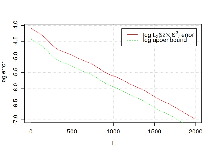
Some additional numerical studies of the dependence on time and the parameters are given in Appendix C. The code in the folder ”Research materials” from https://sites.google.com/site/olenkoandriy/ can be used to obtain maps of realisations for different parameters that were not included in this section or to experiment with other combinations of the parameters.
8 Conclusions and future work
This research provides physical motivation and justification for stochastic diffusion models in CMB studies. The Cauchy problem with random initial conditions for hyperbolic diffusion equations on the unit sphere was considered. Properties of exact and approximate solutions were investigated. The numerical studies illustrated the obtained results and examined the sensitivity of solutions to parameters using the CMB data. They indicated that the model is flexible enough to capture some of the statistical properties of the CMB.
It was shown that properties of the solutions are determined by the decay of the angular power spectrum. The analysis of the CMB covariance revealed that dependencies between CMB observations rapidly decrease with angular distance between their locations. The numerical studies demonstrated that the CMB evolution under this SPDE model results in most significant changes of CMB temperature spectrum at the high frequency range in the first place. At the same time relatively large changes of at high CMB frequencies have little impact on the covariance functions and CMB maps that remain almost unchanged. The contribution of high frequency components to the CMB field is decreasing with at a faster rate than a power-law.
The sensitivity analysis to parameters at the lower frequency spectrum range demonstrated that changes in time and the parameters and have a substantial impact on the error, while showed almost no effect.
It would be interesting to extend the obtained results and
- (1)
apply this model to backward studies of CMB;
- (2)
compare this model with other possible evolution scenarios;
- (3)
investigate 3-dimensional SPDEs as the next generation CMB experiment, CMB-S4, will be collecting 3D spatial data;
- (4)
explore applications to other spherical data in physics and earth sciences.
Acknowledgements.
This research was supported under the Australian Research Council’s Discovery Project DP160101366. N. Leonenko was supported in part by Cardiff Incoming Visiting Fellowship Scheme, International Collaboration Seedcorn Fund, Data Innovation URI Seedcorn Fund. We are also grateful for the use of data of the Planck/ESA mission from the Planck Legacy Archive. The authors are also grateful to the referees for their careful reading of the paper and suggestions that helped to improve the paper.Appendix A: Diffusion length of a local disturbance.
Consider a density disturbance of total mass originating at the origin. The well-known point source solution to linear diffusion in three space dimensions is given by
The density level set at some low significance value is at
so
The level set reaches its maximum extent when , implying so the diffusion length is
For example, for a mass disturbance the size of a solar mass, and a neutron diffusion length of 0.3 light-year at the temperature of neutrino dissociation from weak nuclear interactions, estimated from Applegate and Kurki, the marginal disturbance density is around 1 solar mass per cubic light year. This is meant to have occurred at a time when the cosmological expansion factor was less than , so after expansion to the current level, the equivalent marginal density would be less than one nucleon mass per cubic metre, around the current mean density of the universe.
Appendix B: Proofs.
Proof of Theorem 4.1. By substituting (19) into equation (15) and using (18), we obtain
| (31) |
To find particular solutions of (31), we need to solve the ordinary differential equation
| (32) |
The initial conditions for this equation can be determined from (20) and (16) and they are
| (33) |
The characteristic equation of (32) is with the roots Therefore, the general solution of equation (32) is given by the formula:
where are some constants. From the initial conditions in (33) we obtain
Note that the multiplier of on the right-hand side of (34) equals
By substituting this expression into (34), we get
Finally, using and rewriting the Green function we obtain the statement of the theorem.
Proof of Theorem 4.2. The solution of the initial value problem (22) - (24) can be written as a spherical convolution of the Green function from Section 4 and the random field if the corresponding Laplace series converges in the Hilbert space
Let the two functions and on the sphere belong to the space and have the Fourier-Laplace coefficients
Recall (see, i.e., Dunkel) that their non-commutative spherical convolution is defined as the Laplace series
| (35) |
with the Fourier-Laplace coefficients given by
provided that the series (35) converges in the corresponding Hilbert space.
Thus, the random solution of equation (22) with the initial values determined by (23) and (24) can be written as a spherical random field with the following Laplace series representation
| (36) |
provided that this series is convergent in the Hilbert space where is given by Theorem 4.1 and is given by (23). The complex Gaussian random variables are given by
where and
It gives the first statement of the theorem.
By the addition formula for spherical harmonics (see, i.e., MarinucciPeccati13, p.66)
| (37) |
where is the -th Legendre polynomial (see (8)), and is the angular distance between the points and on
Using (10) we obtain that the random field is isotropic if and only if the covariance structure of the solution (25) can be written in the form
Noting that only a finite number of terms is non-zero, and there is a constant such that we obtain that condition (38) follows from (13). This condition on the angular spectrum guarantees the convergence of the series (36) in the Hilbert space
Proof of Theorem 5.1. The approximation is a centered Gaussian random field, i.e. for all and Therefore,
| (39) |
Then, applying Chebyshev’s inequality, we get the upper bound in (ii).
Finally, (iii) follows from statement (ii) and the Borel–Cantelli lemma as
Proof of Theorem 6.1. Let belong to a bounded neighbourhood of the origin. It follows from (14), (26), (27), (28) and (37) that
| (41) |
We start by showing how to estimate the first summand in (41). By (27), for the case we obtain
For we will use the upper bound
By properties of and we get
Then, applying (27) and noting that only a finite number of is non-vanished (namely, only if ) we obtain the following estimates
Applying the above estimates to (41) we obtain
which completes the proof.
Appendix C: Sensitivity to parameters.
To further understand the impact of time and the model parameters on the difference of the mean -errors and their upper bound (30) we produced 3d-plots showing the difference as a function of the truncation degree and each parameter provided that other parameters are fixed. These plots are displayed in Figures 15, 15, 15, and 15.

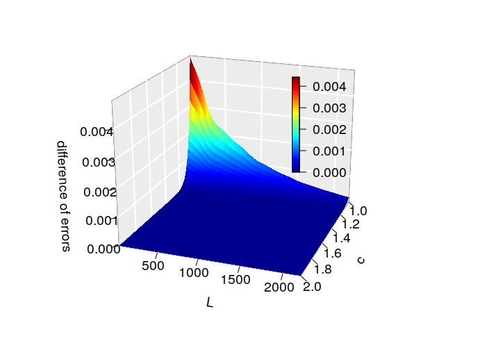
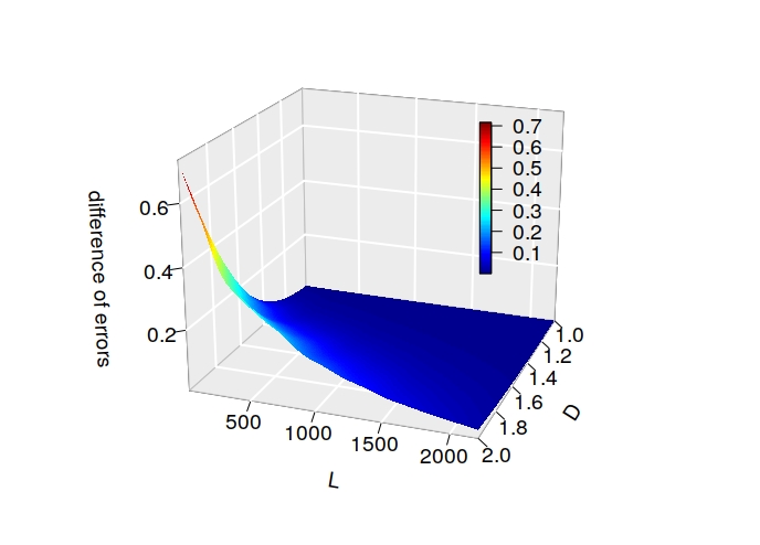
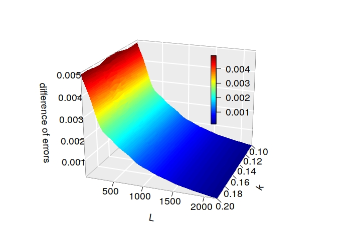
In all cases the difference between the error and its upper bound asymptotically vanish when increases. Figure 15 demonstrates that the difference is a decreasing function of time which is expected as the series representation (25) of the solutions has the multiplication factor exponentially decaying in time. The differences are extreme at the origin and decrease when time or the parameter increases, see Figure 15. For the parameter the situation depicted in Figure 15 is opposite and the difference is increasing in which is expected as the multiplication factor is exponentially decaying in Finally, Figure 15 suggests that the parameter seems have no substantial impact on the difference.
References
- (1) Adam, R. et al.: Planck 2015 results. I, Overview of products and scientific results, Astron. Astrophys. 594, A16 (2016)
- (2) Ade, P.A.R. et al.: Planck 2015 results. XVI, Isotropy and statistics of the CMB, Planck Collaboration, Astron. Astrophys. 594, A16 (2016)
- (3) Ali, Y. M., Zhang, L. C.: Relativistic heat conduction. Int. J. Heat Mass Trans. 48 (12), 2397-2406 (2005)
- (4) Anh, V. V., Leonenko, N. N. Spectral analysis of fractional kinetic equations with random data. J. Stat. Phys. 104 (5-6), 1349-1387 (2001)
- (5) Anh, V. V., Broadbridge, P., Olenko, A., Wang, Y. G.: On approximation for fractional stochastic partial differential equations on the sphere. Stoch. Environ. Res. Risk Assess. 32, 2585-2603 (2018)
- (6) Applegate, J. H., Hogan, C. J., Scherrer, R. J.: Cosmological baryon diffusion and nucleosynthesis. Phys. Rev. D. 35 (4), 1151-1159 (1987)
- (7) Barrow, J. D., Scherrer, R. J.: Constraining density fluctuations with big-bang nucleosynthesis in the era of precision cosmology. Phys. Rev. D 98 (4), art. 043534 (2018)
- (8) Berg, E. J.: Heaviside’s Operational Calculus. McGraw-Hill, New York (1936)
- (9) Birrell, N. D., Davies, P. C. W.: Quantum Fields in Curved Space. Cambridge University Press, London (1984)
- (10) Bjørken, J. D., Drell, S. D. Relativistic Quantum Mechanics. McGraw-Hill, New York (1964)
- (11) Broadbridge, P., Zulkowski, P.: Dark energy states from quantization of boson fields in a universe with unstable modes. Rep. On Math. Phys. 7 (1), 27-40 (2006)
- (12) Carslaw, H. S., Jaeger, J. C.: Conduction of Heat in Solids. Oxford University Press, London (1959)
- (13) Cattaneo, C. R.: Sur une forme de l’équation de la chaleur éliminant le paradoxe d’une propagation instantanée. Comptes Rendus. 247 (4), 431-433 (1958)
- (14) Dodelson, S.: Modern Cosmology. Academic Press, New York (2003)
- (15) Dunkel, J., Hänggi, P.: Relativistic Brownian motion. Physical Reports, 471, 1-73 (2009)
- (16) Fryer, D., Olenko, A., Li, M.: rcosmo: R Package for Analysis of Spherical, HEALPix and Cosmological Data. submitted (2019) https://arxiv.org/abs/1907.05648
- (17) Fryer, D., Olenko, A., Li, M., Wang, Yu.: rcosmo: Cosmic Microwave Background Data Analysis. R package version 1.0.0. https://CRAN.R-project.org/package=rcosmo (2018)
- (18) Gorski, K.M., Hivon, E., Banday, A.J., Wandelt, B.D., Hansen, F.K., Reinecke, M., Bartelmann, M.: HEALPix: A framework for high-resolution discretization and fast analysis of data distributed on the sphere. Astrophys. J. 622, 759-771 (2005)
- (19) Higgs, P. My Life as a Boson: The story of ”The Higgs”. Internat. J. Modern Physics A 17 (Supp. 01), 86-88 (2002)
- (20) Hirata, C.: The Standard Model - Cosmology. Caltech lecture notes. www.tapir.caltech.edu/~chirata/ph217 (2017)
- (21) Iocco, F., Mangano, G., Miele, G., Pisanti, O., Serpico,P. D.: Primordial nucleosynthesis: from precision cosmology to fundamental physics. Phys. Rep. 472 (1-6), 1-76. (2009)
- (22) Ivanov, A. V., Leonenko, N. N.: Statistical Analysis of Random Fields. Kluwer Academic Publishers, Dordrecht (1989)
- (23) Kolesnik, A. D., Ratanov, N.: Telegraph Processes and Option Pricing. Springer, Heidelberg (2013)
- (24) Kozachenko, Yu. V., Kozachenko, L. F.: Modeling Gaussian isotropic random fields on a sphere. J. Math. Sci. 107, 3751–3757 (2001)
- (25) Kurki-Suonio, H., Jedamzik, K., Matthews, G. J.: Stochastic isocurvature baryon fluctuations, baryon diffusion, and primordial nucleosynthesis. Astrophys. J. 479, 31-39 (1997)
- (26) Lan, X., Xiao, Y.: Regularity properties of the solution to a stochastic heat equation driven by a fractional Gaussian noise on J. Math. Anal. Appl. 476 (1), 27-52 (2019).
- (27) Lang, A., Schwab, C.: Isotropic Gaussian random fields on the sphere: regularity, fast simulation and stochastic partial differential equations. Ann. Appl. Probab. 25, 3047-3094 (2015)
- (28) Leonenko, N.N.: Limit Theorems for Random Fields with Singular Spectrum. Kluwer Academic Publishers, Dordrecht (1999)
- (29) Marinucci, D., Peccati, G.: Random Fields on the Sphere. Representation, Limit Theorems and Cosmological Applications. Cambridge University Press, Cambridge (2011)
- (30) Marinucci, D., Peccati, G.: Mean-square continuity on homogeneous spaces of compact groups. Electron. Commun. Probab. 18, 1-10 (2013)
- (31) NASA/WMAP Science Team: What is the Universe Made of? https://wmap.gsfc.nasa.gov/universe/uni_matter.html
- (32) Schweber, S. An Introduction to Relativistic Quantum Field Theory. Dover, New York (2005)
- (33) Thompson, P. A. Compressible-Fluid Dynamics. McGraw-Hill, New York (1971)
- (34) Terasawa, N., Sato, K.: Neutron diffusion and nucleosynthesis in the inhomogeneous universe. Prog. Theor. Phys. 81 (2), 254-259 (1989)
- (35) Weinberg, S.: Cosmology. Oxford University Press, Oxford (2008)
- (36) Wigner, E. P. On unitary representations of the inhomogeneous Lorentz group. Annals of Mathematics. 40 (1),149-204 (1939)
- (37) Yadrenko, M. I.: Spectral Theory of Random Fields. Optimization Software Inc., New York (1983)