跳到论文正文
W Papers独立论文阅读器 arXiv:1904.12236 论文正文 计算阅读时间 · 0%
引用这篇论文根据当前论文元数据生成,正式投稿前建议核对。


License: CC BY 4.0
arXiv:1904.12236v2 [hep-ph] 29 Apr 2020

Azimuthal asymmetries from θ\theta Vacuum

Weihua Yang Affiliation: Department of Modern Physics, University of Science and Technology of China, Hefei, Anhui 230026, China
Abstract

In this note, we calculate azimuthal asymmetries in terms of fragmentation functions in semi-inclusive electron positron annihilation process. These fragmentation functions are divided into two parts according to the parity even or parity odd properties. We present eight kinds of azimuthal asymmetries and we categorize them for four categories. First, asymmetries comes from both 𝒫\mathcal{P} odd FFs and 𝒫\mathcal{P} even FFs which have same signs (e.g., H1⟂​H¯1⟂+ℋ1⟂​ℋ¯1⟂H^{\perp}_{1}\bar{H}^{\perp}_{1}+\mathcal{H}^{\perp}_{1}\bar{\mathcal{H}}^{\perp}_{1}). Second, asymmetries comes from two interference terms between the 𝒫\mathcal{P} odd FF and 𝒫\mathcal{P} even FF which have opposite signs (e.g., H1⟂​ℋ1⟂−ℋ1⟂​H¯1⟂H^{\perp}_{1}\mathcal{H}^{\perp}_{1}-\mathcal{H}^{\perp}_{1}\bar{H}^{\perp}_{1}). Third, asymmetries comes from both 𝒫\mathcal{P} odd FFs and 𝒫\mathcal{P} even FFs which have opposite signs (e.g., 𝒢1​T⟂​𝒟¯1−D1​T⟂​D¯1\mathcal{G}^{\perp}_{1T}\bar{\mathcal{D}}_{1}-D^{\perp}_{1T}\bar{D}_{1}). Fourth, asymmetries comes from two interference terms between the 𝒫\mathcal{P} odd FF and 𝒫\mathcal{P} even FF which have same signs (H1​T​ℋ¯1⟂+ℋ1​T​H¯1⟂H_{1T}\bar{\mathcal{H}}^{\perp}_{1}+\mathcal{H}_{1T}\bar{H}_{1}^{\perp} ). The 𝒫\mathcal{P}-odd fragmentation functions, e.g., ℋ1⟂\mathcal{H}_{1}^{\perp}, are induced by l​o​c​a​llocal 𝒫\mathcal{P}- and/or 𝒞​𝒫\mathcal{CP}-odd effects which are connected to the tunneling (θ\theta vacuum) events. Due to the 𝒫\mathcal{P}-odd effect, azimuthal asymmetries induced by the effect vanish if all events are summed over but survive on the event-by-event for the interference terms with opposite signs. However, interference terms with same signs survive and can be used to measure/study the 𝒫\mathcal{P}-odd fragmentation functions. Finally, we also calculate hadron polarizations in terms of both the 𝒫\mathcal{P}-even and 𝒫\mathcal{P}-odd fragmentation functions.

I Introduction

Parton distribution functions (PDFs) and fragmentation functions (FFs) are two important quantities in describing the high energy reactions. Both of them are long distance non-perturbative quantities which cannot be calculated with perturbative theory, they are mainly calculated by phenomenological models and parametrized by experiment data Jakob:1997wg; Avakian:2010br; Bacchetta:2001di; Amrath:2005gv; Metz:2002iz; Bacchetta:2007wc; Davidson:2001cc; Ito:2009zc; Matevosyan:2010hh; Matevosyan:2011vj; Matevosyan:2012ga; Dulat:2015mca; Albino:2008fy; canshuhua; deFlorian:1997zj. When three-dimensional, i.e., the transverse momentum dependent (TMD) PDFs and FFs are considered, the sensitive quantities studied in experiments are often different azimuthal asymmetries. In the quantum field theoretical formulation, PDFs and/or FFs are defined by the quark-quark correlators (correlation functions) which are defined as 4×44\times 4 matrices in Dirac space depending on the hadron state. As a result, the correlators can be decomposed by the Dirac matrices, i.e., Γ={I,i​γ5,γμ,γμ​γ5,i​σμ​ν​γ5}\Gamma=\{I,i\gamma^{5},\gamma^{\mu},\gamma^{\mu}\gamma^{5},i\sigma^{\mu\nu}\gamma^{5}\}. The corresponding coefficients can be further decomposed by the Lorentz covariants and scalar functions and these scalar functions are called PDFs and FFs.

Generally, the quark-quark correlator satisfies two constraints, Hermiticity and parity conservation. Hermiticity ensures that all the scalar functions are real while parity conservation strictly limits the numbers of scalar functions. Even though parity violating effects are not expected in perturbative quantum chromodynamics (QCD), the non-trivial θ\theta vacuum may lead to the constraint breakdown tHooft:1976rip; tHooft:1976snw; Jackiw:1976pf; Callan:1976je. The θ\theta term enters in the lagrangian as

ℒθ=θ16​π2​Tr​[Fμ​ν​F~μ​ν]\displaystyle\mathcal{L}_{\theta}=\frac{\theta}{16\pi^{2}}\mathrm{Tr}\big[F_{\mu\nu}\tilde{F}^{\mu\nu}\big] (1)

where Fμ​νF_{\mu\nu} is the gluon field strength tensor and F~μ​ν=εμ​ν​ρ​σ​Fρ​σ/2\tilde{F}^{\mu\nu}=\varepsilon^{\mu\nu\rho\sigma}F_{\rho\sigma}/2. We see that the θ\theta term in lagrangian violates the parity (𝒫\mathcal{P}) and/or charge-parity (𝒞​𝒫\mathcal{CP}) symmetries. However the measurements of electric dipole moment of neutron indicate that the parity (𝒫\mathcal{P}) violation is l​o​c​a​llocal Baker:2006ts. Even though QCD is l​o​c​a​llocal 𝒫\mathcal{P} violated, Kharzeev, Pisarski and Tytgat have shown it can be directly observed Kharzeev:1998kz. In heavy ion collisions, it also leads to the famous chiral magnetic effect Kharzeev:2004ey; Kharzeev:2007jp; Fukushima:2008xe. Furthermore, Efremov, Kharzeev and Kang also discussed the l​o​c​a​llocal 𝒫\mathcal{P} odd effect in fragmentation process. In this case, the 𝒫\mathcal{P} odd FFs emerge and they argued that the effect can be detected in experiments via physical observables, e.g., handedness correlation and azimuthal asymmetries Efremov:1995ff; Kang:2010qx.

Electron positron annihilation process is regard as the most cleanest place to study the FFs, because in this process there are no hadronic effects in initial states. As we mentioned before the sensitive quantities studied in experiments are often different azimuthal asymmetries when TMD FFs are considered. In ref. Kang:2010qx, Kang and Kharzeev derived the most general form of the FF for quarks fragmenting into spin-0 hadrons (pseudoscalars) at leading twist. Without the parity constraint they found two more 𝒫\mathcal{P} odd FFs which are related to two azimuthal asymmetries, i.e., cos⁡2​ϕ\cos 2\phi and sin⁡2​ϕ\sin 2\phi. They presented a estimation of the magnitude of the sin⁡2​ϕ\sin 2\phi asymmetry, they found I⁡(θ¯,z1,z2)∼1.5%I(\bar{\theta},z_{1},z_{2})\sim 1.5\%. This is a relative large asymmetry and can be detected. In this note we extend the calculation to spin-1/2 dihadron production. We calculate the azimuthal asymmetries for unpolarized, single-spin asymmetries and double spin asymmetries, respectively. We also calculate the hadron polarizations.

This note is organized as follows. In Sect. II we present the kinematics of the semi-inclusive electron positron annihilation (SIA) precess and the conventions and notations used in this note. In Sect. III we present the decompositions of the correlation functions as well as the complete hadronic tensor. Our calculation results are shown in Sect. IV. And a brief summary will be given in Sect. V.

II Kinematics

In this section we present the kinematics of the SIA process, see Fig. 1. Here SIA process denotes that two hadron are produced in two back-to back-jets in electron positron annihilation preocess, respectively. In this note we only consider the electromagnetic interaction for distinguishing the 𝒫\mathcal{P}-odd effect in QCD from weak interaction theory. The differential cross section of SIA process can be written as contraction of the leptonic tensor and hadronic tensor, i.e.,

2​E1​E2​d​σd3​p→1​d3​p→2=Nc​αe​m2​eq2s​Q4​Lμ​ν​(l1,l2)​Wμ​ν​(p1,p2),\displaystyle\frac{2E_{1}E_{2}d\sigma}{d^{3}\vec{p}_{1}d^{3}\vec{p}_{2}}=\frac{N_{c}\alpha^{2}_{em}e_{q}^{2}}{sQ^{4}}L_{\mu\nu}(l_{1},l_{2})W^{\mu\nu}(p_{1},p_{2}), (2)

where NcN_{c} denotes the color factor, αe​m\alpha_{em} is the fine structure constant and eqe_{q} is the electric charge of quark qq. s=Q2=q2=(l1+l2)2s=Q^{2}=q^{2}=(l_{1}+l_{2})^{2}. The leptonic tensor is given by

Lμ​ν​(l1,l2)\displaystyle L_{\mu\nu}(l_{1},l_{2}) =14​Tr​[l̸1​γμ​l̸2​γν]\displaystyle=\frac{1}{4}\mathrm{Tr}\left[\not{l}_{1}\gamma_{\mu}\not{l}_{2}\gamma_{\nu}\right]
=l1​μ​l2​ν+l1​ν​l2​μ−gμ​ν​(l1⋅l2).\displaystyle=l_{1\mu}l_{2\nu}+l_{1\nu}l_{2\mu}-g_{\mu\nu}\left(l_{1}\cdot l_{2}\right). (3)

The operator definition of hadronic tensor is given by

Wμ​ν​(p1,p2)=Δ​∑X⟨0​|Jμ​(0)|​p1,p2;X⟩​⟨p1,p2;X​|Jν​(0)|​0⟩\displaystyle W^{\mu\nu}(p_{1},p_{2})=\Delta\sum_{X}\langle 0|J^{\mu}(0)|p_{1},p_{2};X\rangle\langle p_{1},p_{2};X|J^{\nu}(0)|0\rangle
=∫d2​y​e−i​q​y​∑X⟨0​|Jμ​(0)|​p1,p2;X⟩​⟨p1,p2;X​|Jν​(y)|​0⟩,\displaystyle=\int d^{2}ye^{-iqy}\sum_{X}\langle 0|J^{\mu}(0)|p_{1},p_{2};X\rangle\langle p_{1},p_{2};X|J^{\nu}(y)|0\rangle, (4)

where Δ=δ4​(q−p1−p2−X)\Delta=\delta^{4}(q-p_{1}-p_{2}-X). Besides the Lorentz covariance, the hadronic tensor Wμ​νW_{\mu\nu} satisfies the general constraints imposed by hermiticity, current conservation, and parity conservation in the electromagnetic process, i.e.,

W∗μ​ν​(p1,S1,p2,S2)\displaystyle W^{*\mu\nu}(p_{1},S_{1};p_{2},S_{2}) =Wν​μ​(p1,S1,p2,S2),\displaystyle=W^{\nu\mu}(p_{1},S_{1};p_{2},S_{2}), (5)
qμ​Wμ​ν​(p1,S1,p2,S2)\displaystyle q_{\mu}W^{\mu\nu}(p_{1},S_{1};p_{2},S_{2}) =qν​Wμ​ν​(p1,S1,p2,S2)=0,\displaystyle=q_{\nu}W^{\mu\nu}(p_{1},S_{1};p_{2},S_{2})=0, (6)
Wμ​ν​(p1,S1,p2,S2)\displaystyle W^{\mu\nu}(p_{1},S_{1};p_{2},S_{2}) =Wμ​ν​(p1𝒫,S1𝒫,p2𝒫,S2𝒫),\displaystyle=W_{\mu\nu}(p^{\mathcal{P}}_{1},S^{\mathcal{P}}_{1};p^{\mathcal{P}}_{2},S^{\mathcal{P}}_{2}), (7)

where a vector with the superscript 𝒫\mathcal{P} denotes the result after space reflection such as pμ𝒫=pμp_{\mu}^{\mathcal{P}}=p^{\mu}. From Eq. (4) we know that the hadronic tensor can not be calculated perturbatively because it contains the nonperturbative hadronization process. However, to obtain the cross section, we can decompose the hadronic tensor with the basic Lorentz tensors as shown in ref. Pitonyak:2013dsu; Chen:2016moq. Here we will not repeat the decompositions.

Refer to caption
Figure 1: Semi-inclusive electron positron annihilation process. The momenta of particles are shown in the parenthesises in the figure.
Refer to caption
Figure 2: Semi-inclusive electron positron annihilation process in the lepton center of mass frame.

To calculate the SIA process, we choose the lepton center-of-mass frame where p2p_{2} lies in the positive zz direction, see Fig. 2. In this frame we use the following conventions and notation given in ref. Boer:1997mf. We define

t^μ\displaystyle\hat{t}^{\mu} ≡qμQ,\displaystyle\equiv\frac{q^{\mu}}{Q}, (8)
z^μ\displaystyle\hat{z}^{\mu} ≡Qp2⋅q​p2​qμ=2​p2μz2​Q−qμQ,\displaystyle\equiv\frac{Q}{p_{2}\cdot q}p^{\mu}_{2q}=2\frac{p_{2}^{\mu}}{z_{2}Q}-\frac{q^{\mu}}{Q}, (9)

where we have defined pqμ=pμ−p⋅qq2​qμp_{q}^{\mu}=p^{\mu}-\frac{p\cdot q}{q^{2}}q^{\mu} and the higher twist terms (1/Q21/Q^{2}) is omitted. There are two projectors which can be defined in terms of t^\hat{t} and z^\hat{z}, they are

g⟂μ​ν≡gμ​ν−t^μ​t^ν+z^μ​z^ν,\displaystyle g_{\perp}^{\mu\nu}\equiv g^{\mu\nu}-\hat{t}^{\mu}\hat{t}^{\nu}+\hat{z}^{\mu}\hat{z}^{\nu}, (10)
ε⟂μ​ν≡−ϵμ​ν​ρ​σ​t^ρ​z^σ=1p2⋅q​ϵμ​ν​ρ​σ​p2​ρ​qσ.\displaystyle\varepsilon_{\perp}^{\mu\nu}\equiv-\epsilon^{\mu\nu\rho\sigma}\hat{t}_{\rho}\hat{z}_{\sigma}=\frac{1}{p_{2}\cdot q}\epsilon^{\mu\nu\rho\sigma}p_{2\,\rho}q_{\sigma}. (11)

Then we have p1⟂μ=g⟂μ​ν​p1​νp_{1\perp}^{\mu}=g_{\perp}^{\mu\nu}p_{1\nu}. For convenience, we also define h^μ=p1⟂μ/|p1⟂|\hat{h}^{\mu}=p_{1\perp}^{\mu}/|p_{1\perp}|. FFs are often define with respect to the transverse momentum of the quark, so it would be convenient to define lightlike directions in terms of the momenta of produced hadrons, p1,p2p_{1},p_{2}. Then we have

p1μ≡z1​Q2​nμ+M12z1​Q​2​n¯μ,\displaystyle p_{1}^{\mu}\equiv\frac{z_{1}Q}{\sqrt{2}}n^{\mu}+\frac{M_{1}^{2}}{z_{1}Q\sqrt{2}}\bar{n}^{\mu}, (12)
p2μ≡M22z2​Q​2​nμ+z2​Q2​n¯μ,\displaystyle p_{2}^{\mu}\equiv\frac{M_{2}^{2}}{z_{2}Q\sqrt{2}}n^{\mu}+\frac{z_{2}Q}{\sqrt{2}}\bar{n}^{\mu}, (13)
qμ≡Q2​nμ+Q2​n¯μ+qTμ,\displaystyle q^{\mu}\equiv\frac{Q}{\sqrt{2}}n^{\mu}+\frac{Q}{\sqrt{2}}\bar{n}^{\mu}+q_{T}^{\mu}, (14)

where qT2≡−QT2q_{T}^{2}\equiv-Q_{T}^{2}, M1,M2M_{1},M_{2} are masses of hadron 1 and hadron 2, respectively. Here we have assumed that QT2≪Q2Q_{T}^{2}\ll Q^{2}. n¯\bar{n} and nn are lightlike unit vectors which satisfy n¯⋅n=1\bar{n}\cdot n=1, n¯2=n2=0\bar{n}^{2}=n^{2}=0. In Eq. (9), p2p_{2} is used to define z^\hat{z}, then we have p1⟂μ=−z1​qTμp_{1\perp}^{\mu}=-z_{1}q_{T}^{\mu}. We may also define the projectors in terms of n¯,n\bar{n},n,

gTμ​ν≡gμ​ν−n¯μ​nν−n¯ν​nμ,\displaystyle g^{\mu\nu}_{T}\equiv g^{\mu\nu}-\bar{n}^{\mu}n^{\nu}-\bar{n}^{\nu}n^{\mu}, (15)
εTμ​ν≡εμ​ν​ρ​σ​n¯ρ​nσ.\displaystyle\varepsilon^{\mu\nu}_{T}\equiv\varepsilon^{\mu\nu\rho\sigma}\bar{n}_{\rho}n_{\sigma}. (16)

We see that the p​e​r​p​e​n​d​i​c​u​l​a​rperpendicular vectors and tensors (labeled by ⟂\perp) are different from the t​r​a​n​s​v​e​r​s​etransverse vectors and tensors (labeled by TT). They can be connected by the following equations, e.g.,

gTμ​ν=g⟂μ​ρ​gT​ρν−QTQ​(z^+t^)​h^μ,\displaystyle g_{T}^{\mu\nu}=g_{\perp}^{\mu\rho}g^{\nu}_{T\rho}-\frac{Q_{T}}{Q}(\hat{z}+\hat{t})\hat{h}^{\mu}, (17)
k⟂μ=kTμ−qT⋅kTQ​(z^+t^),\displaystyle k_{\perp}^{\mu}=k_{T}^{\mu}-\frac{q_{T}\cdot k_{T}}{Q}(\hat{z}+\hat{t}), (18)

where qT⋅kT=−𝐪T⋅𝐤Tq_{T}\cdot k_{T}=-\mathbf{q}_{T}\cdot\mathbf{k}_{T}. Using Eq. (18), we can transform the vectors in transverse basis into perpendicular basis to calculate the hadronic tensor and/or cross section. Calculations will be given in the followings.

On the perpendicular basis the lepton tensor can be parameterized as

Lμ​ν=Q22\displaystyle L_{\mu\nu}=\frac{Q^{2}}{2} [−g⟂μ​ν+4y(1−y)z^μz^ν−4y(1−y)x^μx^ν\displaystyle\Big[-g_{\perp}^{\mu\nu}+4y(1-y)\hat{z}^{\mu}\hat{z}^{\nu}-4y(1-y)\hat{x}^{\mu}\hat{x}^{\nu}
−2(1−2y)y⁡(1−y)z^{μx^ν}]\displaystyle-2(1-2y)\sqrt{y(1-y)}\hat{z}^{\{\mu}\hat{x}^{\nu\}}\Big]
=Q2\displaystyle=Q^{2} [−A(y)g⟂μ​ν+2B(y)z^μz^ν−2B(y)(x^μx^ν+12g⟂μ​ν)\displaystyle\Big[-A(y)g_{\perp}^{\mu\nu}+2B(y)\hat{z}^{\mu}\hat{z}^{\nu}-2B(y)\big(\hat{x}^{\mu}\hat{x}^{\nu}+\frac{1}{2}g_{\perp}^{\mu\nu}\big)
−C(y)D(y)z^{μx^ν}],\displaystyle-C(y)D(y)\hat{z}^{\{\mu}\hat{x}^{\nu\}}\Big], (19)

where x^μ=l⟂μ/D⁡(y)​Q\hat{x}^{\mu}=l_{\perp}^{\mu}/D(y)Q, and

A⁡(y)\displaystyle A(y) =12−y+y2,\displaystyle=\frac{1}{2}-y+y^{2}, (20)
B⁡(y)\displaystyle B(y) =y⁡(1−y),\displaystyle=y\,(1-y), (21)
C⁡(y)\displaystyle C(y) =1−2​y,\displaystyle=1-2y, (22)
D⁡(y)\displaystyle D(y) =y⁡(1−y).\displaystyle=\sqrt{y\,(1-y)}. (23)

Eq. (19) can be used to calculated the cross section by contracting with the hadronic tensor obtained in the following.

III Correlation functions and hadronic tensor
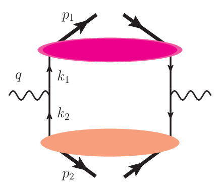
Refer to caption
Figure 3: The hadronic tensor in parton model.

Because the hadronic tensor contains nonperturbative process, it can not be calculated by perturbative theory. In this case we should resort to the parton model Feynman:1969ej; Feynman:1973xc; Bjorken:1969ja. In QCD parton model, see Fig. 3, the hadronic tensor can be rewritten as

Wμ​ν​(p1,p2)=\displaystyle W^{\mu\nu}(p_{1},p_{2})= ∫d2​k1​T(2​π)2​d2​k2​T(2​π)2​δ2​(q→T−k→1​T−k→2​T)\displaystyle\int\frac{d^{2}k_{1T}}{(2\pi)^{2}}\frac{d^{2}k_{2T}}{(2\pi)^{2}}\delta^{2}(\vec{q}_{T}-\vec{k}_{1T}-\vec{k}_{2T})
Tr⁡[Δ¯​(p2,k2​T)​γμ​Δ​(p1,k1​T)​γμ],\displaystyle\mathrm{Tr}\left[\bar{\Delta}(p_{2},k_{2T})\gamma^{\mu}\Delta(p_{1},k_{1T})\gamma^{\mu}\right], (24)

where Δ⁡(z1,k1​T)\Delta(z_{1},k_{1T}) and Δ¯​(z2,k2​T)\bar{\Delta}(z_{2},k_{2T}) are correlation functions and the operator definitions are given by

Δ⁡(p1,k1​T)\displaystyle\Delta(p_{1},k_{1T}) =12​π​∫d​ξ1−​d2​ξ1​T​e−i​k1​ξ1\displaystyle=\frac{1}{2\pi}\int d\xi_{1}^{-}d^{2}\xi_{1T}e^{-ik_{1}\xi_{1}}
∑X⟨0​|ψ⁡(0)|​p1,X⟩​⟨p1,X​|ψ¯​(ξ1)|​0⟩|ξ1+=0,\displaystyle\sum_{X}\langle 0|\psi(0)|p_{1},X\rangle\langle p_{1},X|\bar{\psi}(\xi_{1})|0\rangle|_{\xi_{1}^{+}=0}, (25)
Δ¯​(p2,k2​T)\displaystyle\bar{\Delta}(p_{2},k_{2T}) =12​π​∫d​ξ2−​d2​ξ2​T​e−i​k2​ξ2\displaystyle=\frac{1}{2\pi}\int d\xi_{2}^{-}d^{2}\xi_{2T}e^{-ik_{2}\xi_{2}}
∑X⟨0​|ψ¯​(0)|​p2,X⟩​⟨p2,X​|ψ⁡(ξ2)|​0⟩|ξ2−=0.\displaystyle\sum_{X}\langle 0|\bar{\psi}(0)|p_{2},X\rangle\langle p_{2},X|\psi(\xi_{2})|0\rangle|_{\xi_{2}^{-}=0}. (26)

Equations (25)-(26) are not physical correlation functions, because they are not gauge invariant since the spinor field are not located at the same point. To obtain the gauge invariant correlation functions, gauge links should be taken into consideration. Gauge link (also called Wilson line) is defined as

ℒ⁡(0,∞)=𝒫​e​x​p​[i​g​∫0∞d​z​n​A​(y+z​n)].\displaystyle\mathcal{L}(0,\infty)=\mathcal{P}exp\big[ig\int^{\infty}_{0}dznA(y+zn)\big]. (27)

Armed with the gauge links, the gauge invariant correlation functions are given by,

Ξ^​(p1,k1​T)\displaystyle\hat{\Xi}(p_{1},k_{1T}) =12​π​∫d​ξ1−​d2​ξ1​T​e−i​k1​ξ1​∑X⟨0|​ψ​(0)​ℒ​(0,∞)\displaystyle=\frac{1}{2\pi}\int d\xi_{1}^{-}d^{2}\xi_{1T}e^{-ik_{1}\xi_{1}}\sum_{X}\langle 0|\psi(0)\mathcal{L}(0,\infty)
×|p1,X⟩⟨p1,X|ψ¯(ξ1)ℒ†(ξ,∞)|0⟩|ξ1+=0,\displaystyle\times|p_{1},X\rangle\langle p_{1},X|\bar{\psi}(\xi_{1})\mathcal{L}^{\dagger}(\xi,\infty)|0\rangle|_{\xi_{1}^{+}=0}, (28)
Ξ^¯​(p2,k2​T)\displaystyle\bar{\hat{\Xi}}(p_{2},k_{2T}) =12​π​∫d​ξ2−​d2​ξ2​T​e−i​k2​ξ2​∑X⟨0|​ψ¯​(0)​ℒ†​(0,∞)\displaystyle=\frac{1}{2\pi}\int d\xi_{2}^{-}d^{2}\xi_{2T}e^{-ik_{2}\xi_{2}}\sum_{X}\langle 0|\bar{\psi}(0)\mathcal{L}^{\dagger}(0,\infty)
×|p2,X⟩⟨p2,X|ψ(ξ2)ℒ(ξ,∞)|0⟩|ξ2−=0.\displaystyle\times|p_{2},X\rangle\langle p_{2},X|\psi(\xi_{2})\mathcal{L}(\xi,\infty)|0\rangle|_{\xi_{2}^{-}=0}. (29)

As we have mentioned in Sect. I, these correlation functions given by Eqs. (28)-(29) satisfy the following constraints imposed by Hermiticity and parity conservation, i.e.,

Ξ^†​(p,kT)\displaystyle\hat{\Xi}^{\dagger}(p,k_{T}) =γ0​Ξ^†​(p,kT)​γ0,\displaystyle=\gamma^{0}\hat{\Xi}^{\dagger}(p,k_{T})\gamma^{0}, (30)
Ξ^​(p,kT)\displaystyle\hat{\Xi}(p,k_{T}) =γ0​Ξ^†​(p𝒫,kT𝒫)​γ0.\displaystyle=\gamma^{0}\hat{\Xi}^{\dagger}(p^{\mathcal{P}},k^{\mathcal{P}}_{T})\gamma^{0}. (31)

Correlation functions can not be calculated with perturbative theory because they contain the hadronization information. However, they are 4×44\times 4 matrices in Dirac space and can be decomposed in terms of the Γ\Gamma matrices, i.e., Γ={I,iγ5,γρ,γργ5,iσρ​σγ5\Gamma=\{I,i\gamma^{5},\gamma^{\rho},\gamma^{\rho}\gamma^{5},i\sigma^{\rho\sigma}\gamma^{5}}. The decomposition can be written explicitly as

Ξ^=I​Ξ+i​γ5​Ξ~+γα​Ξα+γα​γ5​Ξ~α+i​σα​β​γ5​Ξα​β.\displaystyle\hat{\Xi}=I\Xi+i\gamma^{5}\tilde{\Xi}+\gamma^{\alpha}\Xi_{\alpha}+\gamma^{\alpha}\gamma^{5}\tilde{\Xi}_{\alpha}+i\sigma^{\alpha\beta}\gamma^{5}\Xi_{\alpha\beta}. (32)

Furthermore, with the parity constraint the coefficients in Eq. (32) can be rewritten as

z​Ξα=n¯α​[D1+εT​k​SM​D1​T⟂],\displaystyle z\Xi_{\alpha}=\bar{n}_{\alpha}\bigg[D_{1}+\frac{\varepsilon_{TkS}}{M}D^{\perp}_{1T}\bigg], (33)
z​Ξ~α=n¯α​[λ​G1​L+kT⋅STM​G1​T⟂],\displaystyle z\tilde{\Xi}_{\alpha}=\bar{n}_{\alpha}\bigg[\lambda G_{1L}+\frac{k_{T}\cdot S_{T}}{M}G^{\perp}_{1T}\bigg], (34)
z​Ξρ​α=n¯α​[εT​k​αM​H1⟂+ST​α​H1​T+kT​αM​H1​S⟂],\displaystyle z\Xi_{\rho\alpha}=\bar{n}_{\alpha}\bigg[\frac{\varepsilon_{Tk\alpha}}{M}H^{\perp}_{1}+S_{T\alpha}H_{1T}+\frac{k_{T\alpha}}{M}H^{\perp}_{1S}\bigg], (35)

at leading twist. We see that Ξ\Xi and Ξ~\tilde{\Xi} do not have leading twist contributions. Here we have defined the shorthanded notation H1​S⟂=λ​H1​L⟂+kT⋅STM​H1​T⟂H^{\perp}_{1S}=\lambda H^{\perp}_{1L}+\frac{k_{T}\cdot S_{T}}{M}H^{\perp}_{1T}. If the parity constraint is released, in other words we consider the 𝒫\mathcal{P} odd effects caused by the non-trivial structure QCD θ\theta vacuum, counterparts of the coefficients in the decompositions can be obtained, they are

z​ΞαP=n¯α​[i​γ5​𝒟1+kT⋅STM​𝒟1​T⟂],\displaystyle z\Xi^{P}_{\alpha}=\bar{n}_{\alpha}\bigg[i\gamma^{5}\mathcal{D}_{1}+\frac{k_{T}\cdot S_{T}}{M}\mathcal{D}^{\perp}_{1T}\bigg], (36)
z​Ξ~αP=n¯α​[−i​γ5​λ​𝒢1​L+εT​k​SM​𝒢1​T⟂],\displaystyle z\tilde{\Xi}^{P}_{\alpha}=\bar{n}_{\alpha}\bigg[-i\gamma^{5}\lambda\mathcal{G}_{1L}+\frac{\varepsilon_{TkS}}{M}\mathcal{G}^{\perp}_{1T}\bigg], (37)
z​Ξρ​αP=n¯α​[kT​αM​ℋ1⟂+εT​S​α​ℋ1​T+εT​k​αM​ℋ1​S⟂],\displaystyle z\Xi^{P}_{\rho\alpha}=\bar{n}_{\alpha}\bigg[\frac{k_{T\alpha}}{M}\mathcal{H}^{\perp}_{1}+\varepsilon_{TS\alpha}\mathcal{H}_{1T}+\frac{\varepsilon_{Tk\alpha}}{M}\mathcal{H}^{\perp}_{1S}\bigg], (38)

where the superscript PP denote the parity violating and ℋ1​S⟂=λ​ℋ1​L⟂+kT⋅STM​ℋ1​T⟂\mathcal{H}^{\perp}_{1S}=\lambda\mathcal{H}^{\perp}_{1L}+\frac{k_{T}\cdot S_{T}}{M}\mathcal{H}^{\perp}_{1T}. Here we call D,G,H,𝒟,𝒢D,G,H,\mathcal{D},\mathcal{G} and ℋ\mathcal{H} fragmentation functions in Eqs. (33)-(38). We also use D,G,HD,G,H to denote the parity conserved FFs and use 𝒟,𝒢,ℋ\mathcal{D},\mathcal{G},\mathcal{H} to denote the parity violated FFs. The 𝒫\mathcal{P}-odd and even FFs can be written in a unified form, in this case the correlation function can be written as

z​Ξ\displaystyle z\Xi =n¯​[D1+λ​𝒢1​L+εT​k​SM​D1​T⟂+kT⋅STM​𝒟1​T⟂]\displaystyle=\not{\bar{n}}\bigg[D_{1}+\lambda\mathcal{G}_{1L}+\frac{\varepsilon_{TkS}}{M}D^{\perp}_{1T}+\frac{k_{T}\cdot S_{T}}{M}\mathcal{D}^{\perp}_{1T}\bigg]
+n¯​γ5​[𝒟1+λ​G1​L+εT​k​SM​𝒢1​T⟂+kT⋅STM​G1​T⟂]\displaystyle+\not{\bar{n}}\gamma^{5}\bigg[\mathcal{D}_{1}+\lambda G_{1L}+\frac{\varepsilon_{TkS}}{M}\mathcal{G}^{\perp}_{1T}+\frac{k_{T}\cdot S_{T}}{M}G^{\perp}_{1T}\bigg]
+iσρ​αγ5n¯ρ[εT​k​αM(H1⟂+ℋ1​S⟂)+ST​αH1​T\displaystyle+i\sigma^{\rho\alpha}\gamma^{5}\bar{n}_{\rho}\bigg[\frac{\varepsilon_{Tk\alpha}}{M}\big(H^{\perp}_{1}+\mathcal{H}^{\perp}_{1S}\big)+S_{T\alpha}H_{1T}
+kT​αM(ℋ1⟂+H1​S⟂)+εT​S​αℋ1​T].\displaystyle~~~~~~~~+\frac{k_{T\alpha}}{M}\big(\mathcal{H}^{\perp}_{1}+H^{\perp}_{1S}\big)+\varepsilon_{TS\alpha}\mathcal{H}_{1T}\bigg]. (39)

We have 16 fragmentation functions, 8 parity conserved and 8 parity violated. For every parity conserved one there is a parity violated one corresponding to it, see Table. 1. Here we should know that D1​T⟂D_{1T}^{\perp} and 𝒢1​T⟂\mathcal{G}_{1T}^{\perp} have the same forms while G1​T⟂G_{1T}^{\perp} and 𝒟1​T⟂\mathcal{D}_{1T}^{\perp} have the same forms.

𝒫\mathcal{P}-even D1D_{1} D1​T⟂D_{1T}^{\perp} G1​LG_{1L} G1​T⟂G_{1T}^{\perp} H1⟂H_{1}^{\perp} H1​TH_{1T} H1​L⟂H_{1L}^{\perp} H1​T⟂H_{1T}^{\perp}
𝒫\mathcal{P}-odd 𝒟1\mathcal{D}_{1} 𝒟1​T⟂\mathcal{D}_{1T}^{\perp} 𝒢1​L\mathcal{G}_{1L}  𝒢1​T⟂\mathcal{G}_{1T}^{\perp}  ℋ1⟂\mathcal{H}_{1}^{\perp}   ℋ1​T\mathcal{H}_{1T}   ℋ1​L⟂\mathcal{H}_{1L}^{\perp}  ℋ1​T⟂\mathcal{H}_{1T}^{\perp}
Table 1: 𝒫\mathcal{P}-even and 𝒫\mathcal{P}-odd FFs.

Since we have all the decompositions of the correlation functions, we can calculate the hadronic tensor. To obtain the complete hadronic tensor, we substitute FFs decomposed in Eq. (39) into Eq. (24) (where correlation functions should be changed to the gauge invariant ones) and carry out the calculations. Thus the complete hadronic tensor in SIA process at leading twist is given by

Wμ​ν=4z1​z2​∫d2​k1​T(2​π)2​d2​k2​T(2​π)2​δ2​(q→T−k→1​T−k→2​T)\displaystyle W^{\mu\nu}=\frac{4}{z_{1}z_{2}}\int\frac{d^{2}k_{1T}}{(2\pi)^{2}}\frac{d^{2}k_{2T}}{(2\pi)^{2}}\delta^{2}(\vec{q}_{T}-\vec{k}_{1T}-\vec{k}_{2T})
×{dTμ​ν{[D1+λ1𝒢1​L+εT​k1​S1MD1​T⟂+k1​T⋅S1​TM𝒟1​T⟂][D¯1+λ2𝒢¯1​L+εT​k2​S2MD¯1​T⟂+k2​T⋅S2​TM𝒟¯1​T⟂]\displaystyle\times\Bigg\{d_{T}^{\mu\nu}\bigg\{\Big[D_{1}+\lambda_{1}\mathcal{G}_{1L}+\frac{\varepsilon_{Tk_{1}S_{1}}}{M}D^{\perp}_{1T}+\frac{k_{1T}\cdot S_{1T}}{M}\mathcal{D}^{\perp}_{1T}\Big]\Big[\bar{D}_{1}+\lambda_{2}\bar{\mathcal{G}}_{1L}+\frac{\varepsilon_{Tk_{2}S_{2}}}{M}\bar{D}^{\perp}_{1T}+\frac{k_{2T}\cdot S_{2T}}{M}\bar{\mathcal{D}}^{\perp}_{1T}\Big]
+[𝒟1+λ1G1​L+εT​k1​S1M𝒢1​T⟂+k1​T⋅S1​TMG1​T⟂][𝒟¯1+λ2G¯1​L+εT​k2​S2M𝒢¯1​T⟂+k2​T⋅S2​TMG¯1​T⟂]}\displaystyle\hskip 22.76219pt+\Big[\mathcal{D}_{1}+\lambda_{1}G_{1L}+\frac{\varepsilon_{Tk_{1}S_{1}}}{M}\mathcal{G}^{\perp}_{1T}+\frac{k_{1T}\cdot S_{1T}}{M}G^{\perp}_{1T}\Big]\Big[\bar{\mathcal{D}}_{1}+\lambda_{2}\bar{G}_{1L}+\frac{\varepsilon_{Tk_{2}S_{2}}}{M}\bar{\mathcal{G}}^{\perp}_{1T}+\frac{k_{2T}\cdot S_{2T}}{M}\bar{G}^{\perp}_{1T}\Big]\bigg\}
−dTμ​νk1​T⋅k2​T+k1​T{μk2​Tν}M1​M2​(H1⟂+ℋ1​S⟂)​(H¯1⟂+ℋ¯1​S⟂)−dTμ​νεT​k1​k2+εT​k1{μk2​Tν}M1​M2​(H1⟂+ℋ1​S⟂)​(ℋ¯1⟂+H¯1​S⟂)\displaystyle-\frac{d_{T}^{\mu\nu}k_{1T}\cdot k_{2T}+k_{1T}^{\{\mu}k_{2T}^{\nu\}}}{M_{1}M_{2}}\big(H^{\perp}_{1}+\mathcal{H}^{\perp}_{1S}\big)\big(\bar{H}^{\perp}_{1}+\bar{\mathcal{H}}^{\perp}_{1S}\big)-\frac{d_{T}^{\mu\nu}\varepsilon_{Tk_{1}k_{2}}+\varepsilon_{Tk_{1}}^{~~~\{\mu}k_{2T}^{\nu\}}}{M_{1}M_{2}}\big(H^{\perp}_{1}+\mathcal{H}^{\perp}_{1S}\big)\big(\bar{\mathcal{H}}^{\perp}_{1}+\bar{H}^{\perp}_{1S}\big)
−dTμ​νk1​T⋅k2​T+k1​T{μk2​Tν}M1​M2​(ℋ1⟂+H1​S⟂)​(ℋ¯1⟂+H¯1​S⟂)−dTμ​νεT​k2​k1+εT​k2{μk1​Tν}M1​M2​(ℋ1⟂+H1​S⟂)​(H¯1⟂+ℋ¯1​S⟂)\displaystyle-\frac{d_{T}^{\mu\nu}k_{1T}\cdot k_{2T}+k_{1T}^{\{\mu}k_{2T}^{\nu\}}}{M_{1}M_{2}}\big(\mathcal{H}^{\perp}_{1}+H^{\perp}_{1S}\big)\big(\bar{\mathcal{H}}^{\perp}_{1}+\bar{H}^{\perp}_{1S}\big)-\frac{d_{T}^{\mu\nu}\varepsilon_{Tk_{2}k_{1}}+\varepsilon_{Tk_{2}}^{~~~\{\mu}k_{1T}^{\nu\}}}{M_{1}M_{2}}\big(\mathcal{H}^{\perp}_{1}+H^{\perp}_{1S}\big)\big(\bar{H}^{\perp}_{1}+\bar{\mathcal{H}}^{\perp}_{1S}\big)
−dTμ​νεT​k1​S2+εT​k1{μS2​Tν}M1​(H1⟂+ℋ1​S⟂)​H¯1​T−dTμ​νk1​T⋅S2​T+k1​T{μS2​Tν}M1​(H1⟂+ℋ1​S⟂)​ℋ¯1​T\displaystyle-\frac{d_{T}^{\mu\nu}\varepsilon_{Tk_{1}S_{2}}+\varepsilon_{Tk_{1}}^{~~~\{\mu}S_{2T}^{\nu\}}}{M_{1}}\big(H^{\perp}_{1}+\mathcal{H}^{\perp}_{1S}\big)\bar{H}_{1T}-\frac{d_{T}^{\mu\nu}k_{1T}\cdot S_{2T}+k_{1T}^{\{\mu}S_{2T}^{\nu\}}}{M_{1}}\big(H^{\perp}_{1}+\mathcal{H}^{\perp}_{1S}\big)\bar{\mathcal{H}}_{1T}
−dTμ​νεT​S2​k1+εT​S2{μk1​Tν}M1​(ℋ1⟂+H1​S⟂)​ℋ¯1​T−dTμ​νk1​T⋅S2​T+k1​T{μS2​Tν}M1​(ℋ1⟂+H1​S⟂)​H¯1​T\displaystyle-\frac{d_{T}^{\mu\nu}\varepsilon_{TS_{2}k_{1}}+\varepsilon_{TS_{2}}^{~~~\{\mu}k_{1T}^{\nu\}}}{M_{1}}\big(\mathcal{H}^{\perp}_{1}+H^{\perp}_{1S}\big)\bar{\mathcal{H}}_{1T}-\frac{d_{T}^{\mu\nu}k_{1T}\cdot S_{2T}+k_{1T}^{\{\mu}S_{2T}^{\nu\}}}{M_{1}}\big(\mathcal{H}^{\perp}_{1}+{H}^{\perp}_{1S}\big)\bar{H}_{1T}
−dTμ​νεT​k2​S1+εT​k2{μS1​Tν}M2​H1​T​(H¯1⟂+ℋ¯1​S⟂)−dTμ​νk2​T⋅S1​T+k2​T{μS1​Tν}M2​H1​T​(ℋ¯1⟂+H¯1​S⟂)\displaystyle-\frac{d_{T}^{\mu\nu}\varepsilon_{Tk_{2}S_{1}}+\varepsilon_{Tk_{2}}^{~~~\{\mu}S_{1T}^{\nu\}}}{M_{2}}H_{1T}\big(\bar{H}^{\perp}_{1}+\bar{\mathcal{H}}^{\perp}_{1S}\big)-\frac{d_{T}^{\mu\nu}k_{2T}\cdot S_{1T}+k_{2T}^{\{\mu}S_{1T}^{\nu\}}}{M_{2}}H_{1T}\big(\bar{\mathcal{H}}^{\perp}_{1}+\bar{H}^{\perp}_{1S}\big)
−dTμ​νεT​S1​k2+εT​S1{μk2​Tν}M2​ℋ1​T​(ℋ¯1⟂+H¯1​S⟂)−dTμ​νk2​T⋅S1​T+k2​T{μS1​Tν}M2​ℋ1​T​(H¯1⟂+ℋ¯1​S⟂)\displaystyle-\frac{d_{T}^{\mu\nu}\varepsilon_{TS_{1}k_{2}}+\varepsilon_{TS_{1}}^{~~~\{\mu}k_{2T}^{\nu\}}}{M_{2}}\mathcal{H}_{1T}\big(\bar{\mathcal{H}}^{\perp}_{1}+\bar{H}^{\perp}_{1S}\big)-\frac{d_{T}^{\mu\nu}k_{2T}\cdot S_{1T}+k_{2T}^{\{\mu}S_{1T}^{\nu\}}}{M_{2}}\mathcal{H}_{1T}\big(\bar{H}^{\perp}_{1}+\bar{\mathcal{H}}^{\perp}_{1S}\big)
−(dTμ​νS1​T⋅S2​T+S1​T{μS2​Tν})H1​TH¯1​T−(dTμ​νεT​S2​S1−εT​S2{μS1​Tν})H1​Tℋ¯1​T\displaystyle-\big(d_{T}^{\mu\nu}S_{1T}\cdot S_{2T}+S_{1T}^{\{\mu}S_{2T}^{\nu\}}\big)H_{1T}\bar{H}_{1T}-\big(d_{T}^{\mu\nu}\varepsilon_{TS_{2}S_{1}}-\varepsilon_{TS_{2}}^{~~~\{\mu}S_{1T}^{\nu\}}\big)H_{1T}\bar{\mathcal{H}}_{1T}
−(dTμ​νS1​T⋅S2​T+S1​T{μS2​Tν})ℋ1​Tℋ¯1​T−(dTμ​νεT​S2​S1−εT​S1{μS2​Tν})ℋ1​TH¯1​T}},\displaystyle-\big(d_{T}^{\mu\nu}S_{1T}\cdot S_{2T}+S_{1T}^{\{\mu}S_{2T}^{\nu\}}\big)\mathcal{H}_{1T}\bar{\mathcal{H}}_{1T}-\big(d_{T}^{\mu\nu}\varepsilon_{TS_{2}S_{1}}-\varepsilon_{TS_{1}}^{~~~\{\mu}S_{2T}^{\nu\}}\big)\mathcal{H}_{1T}\bar{H}_{1T}\bigg\}\Bigg\}, (40)

where dTμ​ν=−gTμ​νd_{T}^{\mu\nu}=-g_{T}^{\mu\nu}. Equation (40) is the complete hadronic tensor which is given in terms of both the 𝒫\mathcal{P} even and 𝒫\mathcal{P} odd fragmentation functions in SIA process. It can be easily checked that the hadronic tensor given in Eq. (40) satisfies the current coservation constraint, i.e., qμ​Wμ​ν=qν​Wμ​ν=0q_{\mu}W^{\mu\nu}=q_{\nu}W^{\mu\nu}=0. Substituting Eq. (40) and Eq. (19) into Eq. (2), we can obtain the complete cross section in SIA process at leading twist.

IV Cross sections and azimuthal asymmetries

In the previous section, we show the complete hadronic tensor at leading twist in SIA process with both parity conserved FFs and parity violated FFs’s contributions. In this section, we present the results by dividing the cross section into three parts according to polarizations of the produced dihadron, i.e., unpolarized part, single hadron polarized part and double hadron polarized part, respectively. The hadronic tensor shown in Eq. (40) is given in the transverse basis, to make Lorentz contraction with the leptonic tensor shown in Eq. (19), we should first transform it into the perpendicular bases. Here we will not present the calculation procedure and only show the final results.

IV.1 Unpolarized cross section and azimuthal asymmetries

First of all we consider the unpolarized case where the hadron produced in final state are pseudoscalar particles or spin-0 particles. The differential cross section of it is given by

2​E1​E2​d​σd3​p1​d3​p2\displaystyle\frac{2E_{1}E_{2}d\sigma}{d^{3}p_{1}d^{3}p_{2}} =8​Nc​αe​m2​eq2Q4​z1​z2[A(y)(𝒞[D1D¯1]−𝒞[𝒟1𝒟¯1])\displaystyle=\frac{8N_{c}\alpha^{2}_{em}e_{q}^{2}}{Q^{4}z_{1}z_{2}}\bigg[A(y)\Big(\mathcal{C}[D_{1}\bar{D}_{1}]-\mathcal{C}[\mathcal{D}_{1}\bar{\mathcal{D}}_{1}]\Big)
−B⁡(y)​cos⁡2​ϕ​𝒞​[w12​H1⟂​H¯1⟂+ℋ1⟂​ℋ¯1⟂M1​M2]\displaystyle-B(y)\cos 2\phi~\mathcal{C}\Big[w_{12}\frac{H^{\perp}_{1}\bar{H}^{\perp}_{1}+\mathcal{H}^{\perp}_{1}\bar{\mathcal{H}}^{\perp}_{1}}{M_{1}M_{2}}\Big]
−B(y)sin2ϕ𝒞[w12H1⟂​ℋ¯1⟂−ℋ1⟂​H¯1⟂M1​M2]],\displaystyle-B(y)\sin 2\phi~\mathcal{C}\Big[w_{12}\frac{H^{\perp}_{1}\bar{\mathcal{H}}^{\perp}_{1}-\mathcal{H}^{\perp}_{1}\bar{H}^{\perp}_{1}}{M_{1}M_{2}}\Big]\bigg], (41)

where the abbreviation 𝒞⁡[D1​D¯1]\mathcal{C}[D_{1}\bar{D}_{1}] denotes a convolution,

𝒞⁡[D1​D¯1]=∫d2​k1​T(2​π)2​d2​k2​T(2​π)2​δ2​(q→T−k→1​T−k→2​T)​D1​D¯1.\displaystyle\mathcal{C}[D_{1}\bar{D}_{1}]=\int\frac{d^{2}k_{1T}}{(2\pi)^{2}}\frac{d^{2}k_{2T}}{(2\pi)^{2}}\delta^{2}(\vec{q}_{T}-\vec{k}_{1T}-\vec{k}_{2T})D_{1}\bar{D}_{1}. (42)

The wight function w12=2​𝐡^⋅𝐤1​T​𝐡^⋅𝐤2​T−𝐤1​T⋅𝐤2​T/M1​M2w_{12}=2\hat{\mathbf{h}}\cdot\mathbf{k}_{1T}\hat{\mathbf{h}}\cdot\mathbf{k}_{2T}-\mathbf{k}_{1T}\cdot\mathbf{k}_{2T}/M_{1}M_{2}. From Eq. (41) we can see that the cos⁡2​ϕ\cos 2\phi terms corresponds to the Collins effect which is the reflection of the Collins function H1⟂H^{\perp}_{1} (H¯1⟂\bar{H}^{\perp}_{1}). Apart from the contribution of the Collins function, there is also contribution of 𝒫\mathcal{P} odd Collins-type function ℋ1⟂\mathcal{H}_{1}^{\perp} (ℋ¯1⟂\bar{\mathcal{H}}_{1}^{\perp}). This azimuthal asymmetry can be written as

AU​Ucos⁡2​ϕ=−B⁡(y)A⁡(y)​𝒞⁡[w12​(H1⟂​H¯1⟂+ℋ1⟂​ℋ¯1⟂)]𝒞⁡[D1​D¯1]−𝒞⁡[𝒟1​𝒟¯1],\displaystyle A_{UU}^{\cos 2\phi}=-\frac{B(y)}{A(y)}\frac{\mathcal{C}\big[w_{12}\big(H^{\perp}_{1}\bar{H}^{\perp}_{1}+\mathcal{H}^{\perp}_{1}\bar{\mathcal{H}}^{\perp}_{1}\big)\big]}{\mathcal{C}[D_{1}\bar{D}_{1}]-\mathcal{C}[\mathcal{D}_{1}\bar{\mathcal{D}}_{1}]}, (43)

where the subscript U​UUU denotes unpolarized cases. The first UU denotes hadron 1 is unpolarized, the same to the second hadron. Often we define the weighted functions, i.e.,

D1​(z)=∫d2​kT(2​π)2​D1​(z,kT),\displaystyle D_{1}(z)=\int\frac{d^{2}k_{T}}{(2\pi)^{2}}D_{1}(z,k_{T}), (44)
H1⟂​(z)=∫d2​kT(2​π)2​|kT|M​H1⟂​(z,kT).\displaystyle H_{1}^{\perp}(z)=\int\frac{d^{2}k_{T}}{(2\pi)^{2}}\frac{|k_{T}|}{M}H_{1}^{\perp}(z,k_{T}). (45)

Then we have

A~U​Ucos⁡2​ϕ=−B⁡(y)A⁡(y)​H1⟂​H¯1⟂+ℋ1⟂​ℋ¯1⟂D1​D¯1−𝒟1​𝒟¯1.\displaystyle\tilde{A}_{UU}^{\cos 2\phi}=-\frac{B(y)}{A(y)}\frac{H^{\perp}_{1}\bar{H}^{\perp}_{1}+\mathcal{H}^{\perp}_{1}\bar{\mathcal{H}}^{\perp}_{1}}{D_{1}\bar{D}_{1}-\mathcal{D}_{1}\bar{\mathcal{D}}_{1}}. (46)

We notice that the sign before two term in the numerator are the same, which means both the Collins function and Collins-type function have positive contributions to the cos⁡2​ϕ\cos 2\phi azimuthal asymmetry. In other words Collins effect (cos⁡2​ϕ\cos 2\phi) may have alternative origins except for the Collins function as indicated in ref. Kang:2010qx. The 𝒫\mathcal{P} odd FFs will complete the extraction of Collins function, in other words the Collins function extracted from experiments data contains ℋ1⟂\mathcal{H}^{\perp}_{1} which is not easily to excluded.

Apart from the cos⁡2​ϕ\cos 2\phi azimuthal asymmetry, we also obtain one special azimuthal asymmetry at leading twist, i.e., sin⁡2​ϕ\sin 2\phi asymmetry. sin⁡2​ϕ\sin 2\phi azimuthal asymmetry arise from the interference of H1⟂H^{\perp}_{1} (H¯1⟂\bar{H}^{\perp}_{1}) and ℋ¯1⟂\bar{\mathcal{H}}^{\perp}_{1} (ℋ1⟂\mathcal{H}^{\perp}_{1}), i.e.,

A~U​Usin⁡2​ϕ=−B⁡(y)A⁡(y)​H1⟂​ℋ¯1⟂−ℋ1⟂​H¯1⟂D1​D¯1−𝒟1​𝒟¯1.\displaystyle\tilde{A}_{UU}^{\sin 2\phi}=-\frac{B(y)}{A(y)}\frac{H^{\perp}_{1}\bar{\mathcal{H}}^{\perp}_{1}-\mathcal{H}^{\perp}_{1}\bar{H}^{\perp}_{1}}{D_{1}\bar{D}_{1}-\mathcal{D}_{1}\bar{\mathcal{D}}_{1}}. (47)

A~U​Usin⁡2​ϕ\tilde{A}_{UU}^{\sin 2\phi} vanishes if only 𝒫\mathcal{P}-even FFs are taken into consideration as discussed in ref. Chen:2016moq. The first term in the numerator corresponds to the interference between Collins function H1⟂H_{1}^{\perp} and 𝒫\mathcal{P}-odd (anti) Collins-type FF ℋ¯1⟂\bar{\mathcal{H}}^{\perp}_{1} fragmented by antiquark while the second terms corresponds to the interference between (anti) Collins function H¯1⟂\bar{H}_{1}^{\perp} and 𝒫\mathcal{P} odd Collins-type FF ℋ1⟂\mathcal{H}^{\perp}_{1} fragmented by quark. We also notice that the signs before these two terms in the numerator are opposite, which means that the effect will vanish when sum over many events. In other words we conclude that the 𝒫\mathcal{P} odd effect only survive on the event-by-event basis.

IV.2 Single hadron polarized cross section and asymmetries

For the single hadron polarized case, we assume that hadron 1 is polarized while hadron 2 is unpolarized, or hadron 1 is spin-1/2 particle while hadron 2 is spin-0 particle. For simplicity, we omit those term which have been shown in Eq. (41). Thus the cross section is given by

2​E1​E2​d​σd3​p1​d3​p2\displaystyle\frac{2E_{1}E_{2}d\sigma}{d^{3}p_{1}d^{3}p_{2}} =8​Nc​αe​m2​eq2Q4​z1​z2{A(y)(𝒞[D1D¯1]−𝒞[𝒟1𝒟¯1])\displaystyle=\frac{8N_{c}\alpha^{2}_{em}e_{q}^{2}}{Q^{4}z_{1}z_{2}}\Bigg\{A(y)\Big(\mathcal{C}[D_{1}\bar{D}_{1}]-\mathcal{C}[\mathcal{D}_{1}\bar{\mathcal{D}}_{1}]\Big)
+A⁡(y)\displaystyle+A(y) {λ1[𝒞[𝒢1​LD¯1]−𝒞[G1​L𝒟¯1]]\displaystyle\bigg\{\lambda_{1}\Big[\mathcal{C}[\mathcal{G}_{1L}\bar{D}_{1}]-\mathcal{C}[{G}_{1L}\bar{\mathcal{D}}_{1}]\Big]
+\displaystyle+ |S1​T|{cos(ϕ−ϕS1)𝒞[w1(𝒟1​T⟂D¯1−G1​T⟂𝒟¯1)]\displaystyle|S_{1T}|\Big\{\cos(\phi-\phi_{S_{1}})\mathcal{C}\big[w_{1}\big(\mathcal{D}^{\perp}_{1T}\bar{D}_{1}-G^{\perp}_{1T}\bar{\mathcal{D}}_{1}\big)\big]
+sin(ϕ−ϕS1)𝒞[w1(𝒢1​T⟂𝒟¯1−D1​T⟂D¯1)]}}\displaystyle\hskip 14.22636pt+\sin(\phi-\phi_{S_{1}})\mathcal{C}\big[w_{1}\big(\mathcal{G}^{\perp}_{1T}\bar{\mathcal{D}}_{1}-D^{\perp}_{1T}\bar{D}_{1}\big)\big]\Big\}\bigg\}
−B⁡(y)\displaystyle-B(y) {λ1sin2ϕ[w12(H1​L⟂H¯1⟂−ℋ1​L⟂ℋ1⟂)]\displaystyle\bigg\{\lambda_{1}\sin 2\phi\big[w_{12}\big(H^{\perp}_{1L}\bar{H}_{1}^{\perp}-\mathcal{H}^{\perp}_{1L}\mathcal{H}^{\perp}_{1}\big)\big]
+λ1​cos⁡2​ϕ​[w12​(ℋ1​L⟂​H¯1⟂+H1​L⟂​ℋ1⟂)]\displaystyle+\lambda_{1}\cos 2\phi\big[w_{12}\big(\mathcal{H}^{\perp}_{1L}\bar{H}_{1}^{\perp}+H^{\perp}_{1L}\mathcal{H}^{\perp}_{1}\big)\big]
+\displaystyle+ |S1​T|{cos(ϕ+ϕS1)𝒞[w2(H1​Tℋ¯1⟂+ℋ1​TH¯1⟂)]\displaystyle|S_{1T}|\Big\{\cos(\phi+\phi_{S_{1}})\mathcal{C}\big[w_{2}\big(H_{1T}\bar{\mathcal{H}}^{\perp}_{1}+\mathcal{H}_{1T}\bar{H}_{1}^{\perp}\big)\big]
+sin⁡(ϕ+ϕS1)​𝒞​[w2​(H1​T​H¯1⟂−ℋ1​T​ℋ¯1⟂)]\displaystyle\hskip 14.22636pt+\sin(\phi+\phi_{S_{1}})\mathcal{C}\big[w_{2}\big(H_{1T}\bar{H}_{1}^{\perp}-\mathcal{H}_{1T}\bar{\mathcal{H}}^{\perp}_{1}\big)\big]
+cos⁡2​ϕ\displaystyle+\cos 2\phi cos⁡(ϕ−ϕS1)​𝒞​[w12​w1​(ℋ1​T⟂​H¯1⟂+H1​T⟂​ℋ¯1⟂)]\displaystyle\cos(\phi-\phi_{S_{1}})\mathcal{C}\big[w_{12}w_{1}\big(\mathcal{H}^{\perp}_{1T}\bar{H}_{1}^{\perp}+H^{\perp}_{1T}\bar{\mathcal{H}}^{\perp}_{1}\big)\big]
+sin⁡2​ϕ\displaystyle+\sin 2\phi cos(ϕ−ϕS1)𝒞[w12w1(ℋ1​T⟂ℋ¯1⟂−H1​T⟂H¯1⟂)]}}},\displaystyle\cos(\phi-\phi_{S_{1}})\mathcal{C}\big[w_{12}w_{1}\big(\mathcal{H}^{\perp}_{1T}\bar{\mathcal{H}}^{\perp}_{1}-H^{\perp}_{1T}\bar{H}_{1}^{\perp}\big)\big]\Big\}\bigg\}\Bigg\}, (48)

where the weighted functions w1=𝐡^⋅𝐤1​T/M1w_{1}=\hat{\mathbf{h}}\cdot\mathbf{k}_{1T}/M_{1}, w2=𝐡^⋅𝐤2​T/M2w_{2}=\hat{\mathbf{h}}\cdot\mathbf{k}_{2T}/M_{2}. From Eq. (48) we can see that the transverse polarization part vanish when integrate over the transverse momenta. However, we here need to the consider azimuthal asymmetries and the transverse momenta should not be integrated over except for weighted integrals. Here we have,

AT​Usin⁡(ϕ−ϕS1)=𝒞⁡[w1​(𝒢1​T⟂​𝒟¯1−D1​T⟂​D¯1)]𝒞⁡[D1​D¯1]−𝒞⁡[𝒟1​𝒟¯1],\displaystyle A_{TU}^{\sin(\phi-\phi_{S_{1}})}=\frac{\mathcal{C}\big[w_{1}\big(\mathcal{G}^{\perp}_{1T}\bar{\mathcal{D}}_{1}-D^{\perp}_{1T}\bar{D}_{1}\big)\big]}{\mathcal{C}[D_{1}\bar{D}_{1}]-\mathcal{C}[\mathcal{D}_{1}\bar{\mathcal{D}}_{1}]}, (49)
AT​Ucos⁡(ϕ−ϕS1)=𝒞⁡[w1​(𝒟1​T⟂​D¯1−G1​T⟂​𝒟¯1)]𝒞⁡[D1​D¯1]−𝒞⁡[𝒟1​𝒟¯1].\displaystyle A_{TU}^{\cos(\phi-\phi_{S_{1}})}=\frac{\mathcal{C}\big[w_{1}\big(\mathcal{D}^{\perp}_{1T}\bar{D}_{1}-G^{\perp}_{1T}\bar{\mathcal{D}}_{1}\big)\big]}{\mathcal{C}[D_{1}\bar{D}_{1}]-\mathcal{C}[\mathcal{D}_{1}\bar{\mathcal{D}}_{1}]}. (50)

From Eq. (49) we can see that AU​Lsin⁡(ϕ−ϕS1)A_{UL}^{\sin(\phi-\phi_{S_{1}})} corresponds to the Sivers effect in fragmentation process since this azimuthal asymmetry comes from the FFs D1​T⟂​D¯1D^{\perp}_{1T}\bar{D}_{1}. But we see the two terms in the numerator have opposite signs which means that the 𝒫\mathcal{P} odd FFs 𝒢1​T⟂​𝒟¯1\mathcal{G}^{\perp}_{1T}\bar{\mathcal{D}}_{1} have negative contribution to this asymmetry relative to D1​T⟂​D¯1D^{\perp}_{1T}\bar{D}_{1}. Thus the 𝒫\mathcal{P} odd FFs can reduce the magnitude of the asymmetry. However, azimuthal asymmetry AU​Lcos⁡(ϕ−ϕS1)A_{UL}^{\cos(\phi-\phi_{S_{1}})} comes from the interference of the 𝒫\mathcal{P}-odd FF(s) 𝒟1​T⟂​(𝒟¯1)\mathcal{D}^{\perp}_{1T}(\bar{\mathcal{D}}_{1}) and 𝒫\mathcal{P}-even FF(s) D¯1​(G1​T⟂)\bar{D}_{1}(G^{\perp}_{1T}) and it only survive event-by-event basis as we have discussed for Eq. (46).

Besides, we can also calculate the other two azimuthal asymmetries which are generated from the chiral-odd FFs. (The following two azimuthal asymmetries are not the right simplified ones, we show them here for direct impression.) They are given by,

AT​Usin⁡(ϕ+ϕS1)=−𝒞⁡[w2​(H1​T​H¯1⟂−ℋ1​T​ℋ¯1⟂)]𝒞⁡[D1​D¯1]−𝒞⁡[𝒟1​𝒟¯1],\displaystyle A_{TU}^{\sin(\phi+\phi_{S_{1}})}=-\frac{\mathcal{C}\big[w_{2}\big(H_{1T}\bar{H}_{1}^{\perp}-\mathcal{H}_{1T}\bar{\mathcal{H}}^{\perp}_{1}\big)\big]}{\mathcal{C}[D_{1}\bar{D}_{1}]-\mathcal{C}[\mathcal{D}_{1}\bar{\mathcal{D}}_{1}]}, (51)
AT​Ucos⁡(ϕ+ϕS1)=−𝒞⁡[w2​(H1​T​ℋ¯1⟂+ℋ1​T​H¯1⟂)]𝒞⁡[D1​D¯1]−𝒞⁡[𝒟1​𝒟¯1].\displaystyle A_{TU}^{\cos(\phi+\phi_{S_{1}})}=-\frac{\mathcal{C}\big[w_{2}\big(H_{1T}\bar{\mathcal{H}}^{\perp}_{1}+\mathcal{H}_{1T}\bar{H}_{1}^{\perp}\big)\big]}{\mathcal{C}[D_{1}\bar{D}_{1}]-\mathcal{C}[\mathcal{D}_{1}\bar{\mathcal{D}}_{1}]}. (52)

We can see these two asymmetries are related to the transverse polarization transformation function H1​TH_{1T} and Collins function H1⟂H_{1}^{\perp}. Similar to AL​Usin⁡(ϕ−ϕS1)A_{LU}^{\sin(\phi-\phi_{S_{1}})}, the contribution of 𝒫\mathcal{P} odd FFs ℋ1​T​ℋ¯1⟂\mathcal{H}_{1T}\bar{\mathcal{H}}^{\perp}_{1} can reduce the contribution from 𝒫\mathcal{P} even FFs H1​T​H¯1⟂H_{1T}\bar{H}_{1}^{\perp}, since they have different signs. It is interesting to see that the interference two terms contributing to azimuthal asymmetry AL​Ucos⁡(ϕ+ϕS1)A_{LU}^{\cos(\phi+\phi_{S_{1}})} have both positive contributions and they can survive even summing over many events. At leading twist, AT​Ucos⁡(ϕ+ϕS1)A_{TU}^{\cos(\phi+\phi_{S_{1}})} vanishes for parity violated reason, see ref Chen:2016moq. Thus AT​Ucos⁡(ϕ+ϕS1)A_{TU}^{\cos(\phi+\phi_{S_{1}})} is important for determining the 𝒫\mathcal{P}-odd FFs by measuring the azimuthal asymmetry at leading twist.

IV.3 Double hadron polarized cross section and asymmetries

For the double hadron polarized case, we consider two spin-1/2 hadrons in the final states, there are 54 terms. For simplicity, we only consider the integrated cross section and only a few of them are left which are given by

d​σd​z1​d​z2​d​y=4​π​Nc​eq2​αe​m2Q2[A(y)(D1D¯1−𝒟1𝒟¯1)\displaystyle\frac{d\sigma}{dz_{1}dz_{2}dy}=\frac{4\pi N_{c}e_{q}^{2}\alpha_{em}^{2}}{Q^{2}}\Big[A(y)\big(D_{1}\bar{D}_{1}-\mathcal{D}_{1}\bar{\mathcal{D}}_{1}\big)
−A⁡(y)​λ1​λ2​(G1​L​G¯1​L−𝒢1​L​𝒢¯1​L)\displaystyle\hskip 71.13188pt-A(y)\lambda_{1}\lambda_{2}\big(G_{1L}\bar{G}_{1L}-\mathcal{G}_{1L}\bar{\mathcal{G}}_{1L}\big)
−B⁡(y)​|S1​T|​|S2​T|​cos⁡(ϕS1+ϕS2)​(H1​T​H¯1​T+ℋ1​T​ℋ¯1​T)\displaystyle-B(y)|S_{1T}||S_{2T}|\cos(\phi_{S_{1}}+\phi_{S_{2}})\big(H_{1T}\bar{H}_{1T}+\mathcal{H}_{1T}\bar{\mathcal{H}}_{1T}\big)
−B(y)|S1​T||S2​T|sin(ϕS1+ϕS2)(H1​Tℋ¯1​T−ℋ1​TH¯1​T)].\displaystyle-B(y)|S_{1T}||S_{2T}|\sin(\phi_{S_{1}}+\phi_{S_{2}})\big(H_{1T}\bar{\mathcal{H}}_{1T}-\mathcal{H}_{1T}\bar{H}_{1T}\big)\Big]. (53)

Here we have used

d3​p1​d3​p2/E1​E2\displaystyle d^{3}p_{1}d^{3}p_{2}/E_{1}E_{2} =(d​z1/z1)​(z2​Q2​d​z2/4)​d​𝐩1⟂​d​Ω2\displaystyle=(dz_{1}/z_{1})(z_{2}Q^{2}dz_{2}/4)d\mathbf{p}_{1\perp}d\Omega_{2}
=π​Q2​z1​z2​d​z1​d​z2​d​y​d2​𝐪T.\displaystyle=\pi Q^{2}z_{1}z_{2}dz_{1}dz_{2}dyd^{2}\mathbf{q}_{T}. (54)

In Eq. (53), there are two azimuthal asymmetries which correspond to the double spin asymmetries.

A~T​Tcos⁡(ϕS1+ϕS2)=−B⁡(y)A⁡(y)​H1​T​H¯1​T+ℋ1​T​ℋ¯1​TD1​D¯1−𝒟1​𝒟¯1,\displaystyle\tilde{A}_{TT}^{\cos(\phi_{S_{1}}+\phi_{S_{2}})}=-\frac{B(y)}{A(y)}\frac{H_{1T}\bar{H}_{1T}+\mathcal{H}_{1T}\bar{\mathcal{H}}_{1T}}{D_{1}\bar{D}_{1}-\mathcal{D}_{1}\bar{\mathcal{D}}_{1}}, (55)
A~T​Tsin⁡(ϕS1+ϕS2)=−B⁡(y)A⁡(y)​H1​T​ℋ¯1​T−ℋ1​T​H¯1​TD1​D¯1−𝒟1​𝒟¯1.\displaystyle\tilde{A}_{TT}^{\sin(\phi_{S_{1}}+\phi_{S_{2}})}=-\frac{B(y)}{A(y)}\frac{H_{1T}\bar{\mathcal{H}}_{1T}-\mathcal{H}_{1T}\bar{H}_{1T}}{D_{1}\bar{D}_{1}-\mathcal{D}_{1}\bar{\mathcal{D}}_{1}}. (56)

First of all we consider the asymmetry A~T​Tcos⁡(ϕS1+ϕS2)\tilde{A}_{TT}^{\cos(\phi_{S_{1}}+\phi_{S_{2}})}. We find that both H1​T​H¯1​TH_{1T}\bar{H}_{1T} and ℋ1​T​ℋ¯1​T\mathcal{H}_{1T}\bar{\mathcal{H}}_{1T} have contributions to this asymmetry which means A~T​Tcos⁡(ϕS1+ϕS2)\tilde{A}_{TT}^{\cos(\phi_{S_{1}}+\phi_{S_{2}})} has one more origin and it will complicate the extraction of the transverse polarization transformation function H1​TH_{1T}. This is the same to Collins asymmetry, A~U​Ucos⁡2​ϕ\tilde{A}_{UU}^{\cos 2\phi}. The asymmetry A~T​Tsin⁡(ϕS1+ϕS2)\tilde{A}_{TT}^{\sin(\phi_{S_{1}}+\phi_{S_{2}})}, similar to A~U​Usin⁡2​ϕ\tilde{A}_{UU}^{\sin 2\phi}, arise from the two interference terms with opposite signs. So it can only survive on event-by-event basis.

So far we present eight kinds of azimuthal asymmetries. We can divide them into four parts according to the FFs’ contributions.

  • •

    A~U​Ucos⁡2​ϕ\tilde{A}_{UU}^{\cos 2\phi} and A~T​Tcos⁡(ϕS1+ϕS2)\tilde{A}_{TT}^{\cos(\phi_{S_{1}}+\phi_{S_{2}})}. In this part, both the 𝒫\mathcal{P} odd FFs and 𝒫\mathcal{P} even FFs have positive contributions which means these kinds of azimuthal asymmetries have two origins.

  • •

    A~U​Usin⁡2​ϕ\tilde{A}_{UU}^{\sin 2\phi}, A~T​Ucos⁡(ϕ−ϕS1)\tilde{A}_{TU}^{\cos(\phi-\phi_{S_{1}})} and A~T​Tsin⁡(ϕS1+ϕS2)\tilde{A}_{TT}^{\sin(\phi_{S_{1}}+\phi_{S_{2}})}. In this part, asymmetries comes from the interference between the 𝒫\mathcal{P} odd FF and 𝒫\mathcal{P} even FF and terms in the numerator have opposite signs which means these azimuthal asymmetries only survive event-by-event.

  • •

    A~T​Usin⁡(ϕ−ϕS1)\tilde{A}_{TU}^{\sin(\phi-\phi_{S_{1}})} and AT​Usin⁡(ϕ+ϕS1)A_{TU}^{\sin(\phi+\phi_{S_{1}})}. These asymmetries are from both the 𝒫\mathcal{P} odd FFs and 𝒫\mathcal{P} even FFs but these two terms have opposite sign. In other words, the 𝒫\mathcal{P} odd FFs can reduce the effect generated by 𝒫\mathcal{P} even FFs.

  • •

    AT​Ucos⁡(ϕ+ϕS1)A_{TU}^{\cos(\phi+\phi_{S_{1}})}. This kind of azimuthal asymmetry is very special. The interference two terms contributing to azimuthal asymmetry AL​Ucos⁡(ϕ+ϕS1)A_{LU}^{\cos(\phi+\phi_{S_{1}})} have both positive contributions and they can survive even summing over many events. This is important for determining the 𝒫\mathcal{P}-odd FFs by measuring the azimuthal asymmetry at leading twist.

IV.4 Hadron polarizations

In the previous sections we considered azimuthal asymmetries which can be detected directly in SIA experiments. If the spin of hadrons measured in the final state is not zero, the hadron polarization can be measured. For simplicity, in this part we only consider the one hadron polarized case. The hadron polarizations can be calculated in three steps. The first one is to illustrate the probability interpretation, the second is to calculate eigenvalues and the third is the to calculate hadron polarizations. In the following we will take ⟨STx⟩\langle S_{T}^{x}\rangle for example to illustrate the calculations.

Hadron polarization ⟨STx⟩\langle S_{T}^{x}\rangle, in general, denotes the probability of the hadrons in the spin STxS_{T}^{x} state. For a system of hadrons, we use spin density matrix to describe the polarization. The spin density matrix can be written as

ρ=∑m,n|n⟩​⟨n|ρ|m⟩​⟨m|=∑m,nTr⁡[ρ⁡|m⟩​⟨n|]​|n⟩​⟨m|,\displaystyle\rho=\sum_{m,n}|n\rangle\langle n|~\rho~|m\rangle\langle m|=\sum_{m,n}\mathrm{Tr}\big[\rho|m\rangle\langle n|\big]|n\rangle\langle m|, (57)

where |m⟩,|n⟩|m\rangle,|n\rangle are eigenstates of corresponding spin operators and P≡Tr⁡[ρ​|m⟩​⟨n|]P\equiv\mathrm{Tr}\big[\rho|m\rangle\langle n|\big] is the probability of finding one of these states. The spin operator can be defined in arbitrary direction, i.e.,

Σi​n^i=Σx​sin⁡θ​cos⁡ϕ+Σy​sin⁡θ​sin⁡ϕ+Σz​cos⁡θ,\displaystyle\Sigma^{i}\hat{n}^{i}=\Sigma^{x}\sin\theta\cos\phi+\Sigma^{y}\sin\theta\sin\phi+\Sigma^{z}\cos\theta, (58)

where θ\theta and ϕ\phi denote the polar and azimuthal angle. Thus the polarization of a system can be calculated as

O=⟨𝒪⟩=Tr⁡[𝒪​ρ],\displaystyle O=\langle\mathcal{O}\rangle=\mathrm{Tr}[\mathcal{O}\rho], (59)

where 𝒪\mathcal{O} denotes any spin operator. Using Eq. (57)-(59), we obtain

⟨STx⟩=P⁡(1,π2,0)−P⁡(−1,π2,0),\displaystyle\langle S_{T}^{x}\rangle=P(1,\frac{\pi}{2},0)-P(-1,\frac{\pi}{2},0), (60)

where P=P⁡(m,θ,ϕ)P=P(m,\theta,\phi) where mm denotes the eigenvalue of the corresponding state. Do not be confused with the eigenstate |m⟩|m\rangle. So ⟨STx⟩\langle S_{T}^{x}\rangle denote the difference of the two probabilities. We can also calculate

⟨λ⟩=P⁡(1,0,0)−P⁡(−1,0,0),\displaystyle\langle\lambda\rangle=P(1,0,0)-P(-1,0,0), (61)
⟨STy⟩=P⁡(1,π2,π2)−P⁡(−1,π2,π2).\displaystyle\langle S_{T}^{y}\rangle=P(1,\frac{\pi}{2},\frac{\pi}{2})-P(-1,\frac{\pi}{2},\frac{\pi}{2}). (62)

Similarly, all the eigenvalues of the system on eigenstates of λ,STx,STy\lambda,S_{T}^{x},S_{T}^{y} can be calculated. They are given in Table. 2.

  |ψz+⟩|\psi_{z+}\rangle   |ψz−⟩|\psi_{z-}\rangle  |ψy+⟩|\psi_{y+}\rangle   |ψy−⟩|\psi_{y-}\rangle   |ψx+⟩|\psi_{x+}\rangle   |ψx−⟩|\psi_{x-}\rangle
λ\lambda 11 −1-1 00 00 00 00
STx~~S_{T}^{x}~~ 00 00 11 −1-1 00 00
STyS_{T}^{y} 00 00 00 00 11 −1-1
Table 2: Eigenvalues of the system on eigenstates of λ,STx,STy\lambda,S_{T}^{x},S_{T}^{y}.

To calculate the hadron polarization, we consider the single hadron polarized case. First of all, we consider the longitudinal polarization. Using Eq. (61) and substituting the corresponding eigenvalues in Table. 2 into Eq. (48), we can obtain the longitudinal polarization of hadron in SIA process,

⟨λ1⟩=𝒞⁡[𝒢1​L​D¯1]−𝒞⁡[G1​L​𝒟¯1]𝒞⁡[D1​D¯1]−𝒞⁡[𝒟1​𝒟¯1].\displaystyle\langle\lambda_{1}\rangle=\frac{\mathcal{C}[\mathcal{G}_{1L}\bar{D}_{1}]-\mathcal{C}[{G}_{1L}\bar{\mathcal{D}}_{1}]}{\mathcal{C}[D_{1}\bar{D}_{1}]-\mathcal{C}[\mathcal{D}_{1}\bar{\mathcal{D}}_{1}]}. (63)

From Eq. (63)we see the longitudinal polarization in SIA process arising form the interference of the 𝒫\mathcal{P} odd FF(s) 𝒢1​L\mathcal{G}_{1L} (𝒟¯1\bar{\mathcal{D}}_{1}) and the 𝒫\mathcal{P} even FF(s) D¯1\bar{D}_{1} (G1​L{G}_{1L}). The signs of the terms in the numerator are opposite which means that the ⟨λ1⟩\langle\lambda_{1}\rangle only survives on event-bey-event basis because the averaged over cross section of many event vanishes.

According to the cross section shown in Eq. (48) we know the transverse polarization cannot be calculate directly. In Fig. 2, we define the plane determined by momenta l1,l2l_{1},l_{2} and p2p_{2} as x−O−zx-O-z plane or lepton-hadron plane. p2p_{2} lies in z-direction while the x-direction is determined by the transverse momenta of leptons as shown. Here we say transverse polarization is the polarization defined with respect to the lepton hadron plane. Chen e​t​a​l.et~al. argued in ref. Chen:2016moq; Yang:2017sxz, the transverse hadron polarization ⟨STx⟩\langle S_{T}^{x}\rangle corresponds to |ST|cosϕS|S_{T}|\cos\phi_{S} while ⟨STy⟩\langle S_{T}^{y}\rangle corresponds to |ST|sinϕS|S_{T}|\sin\phi_{S} and these polarizations vanish in Eq. (48). In fact, the transverse polarization vanish at leading twist but they survive at twist-3 level. However, in ref. Chen:2016moq; Yang:2017sxz, Chen e​t​a​l.et~al. also discussed the transverse polarizations with respect to hadron-hadron place which is defined by the momenta of the two hadrons as shown in Fig. 2. In the case we can define unit vector e→n\vec{e}_{n} and e→t\vec{e}_{t} to label the transverse directions. Here e→n=p→1×p→2/|p→1×p→2|=(−sin⁡ϕ,cos⁡ϕ)\vec{e}_{n}=\vec{p}_{1}\times\vec{p}_{2}/|\vec{p}_{1}\times\vec{p}_{2}|=(-\sin\phi,\cos\phi) and e→t=p→1​T/|p→1​T|=(cos⁡ϕ,sin⁡ϕ)\vec{e}_{t}=\vec{p}_{1T}/|\vec{p}_{1T}|=(\cos\phi,\sin\phi), i.e., the normal and tangent of the hadron-hadron plane, respectively. Thus the transverse hadron polarization STnS_{T}^{n} corresponds to |ST|​sin⁡(ϕS−ϕ)|S_{T}|\sin(\phi_{S}-\phi) while STtS_{T}^{t} corresponds to |ST|​cos⁡(ϕS−ϕ)|S_{T}|\cos(\phi_{S}-\phi). So we can calculate the transverse polarizations with respect to hadron hadron plane.

⟨STn⟩=−𝒞⁡[w1​(𝒢1​T⟂​𝒟¯1−D1​T⟂​D¯1)]𝒞⁡[D1​D¯1]−𝒞⁡[𝒟1​𝒟¯1],\displaystyle\langle S_{T}^{n}\rangle=-\frac{\mathcal{C}\Big[w_{1}\big(\mathcal{G}^{\perp}_{1T}\bar{\mathcal{D}}_{1}-D^{\perp}_{1T}\bar{D}_{1}\big)\Big]}{\mathcal{C}[D_{1}\bar{D}_{1}]-\mathcal{C}[\mathcal{D}_{1}\bar{\mathcal{D}}_{1}]}, (64)
⟨STt⟩=𝒞⁡[w1​(𝒟1​T⟂​D¯1−G1​T⟂​𝒟¯1)]𝒞⁡[D1​D¯1]−𝒞⁡[𝒟1​𝒟¯1].\displaystyle\langle S_{T}^{t}\rangle=\frac{\mathcal{C}\Big[w_{1}\big(\mathcal{D}^{\perp}_{1T}\bar{D}_{1}-G^{\perp}_{1T}\bar{\mathcal{D}}_{1}\big)\Big]}{\mathcal{C}[D_{1}\bar{D}_{1}]-\mathcal{C}[\mathcal{D}_{1}\bar{\mathcal{D}}_{1}]}. (65)

For ⟨STn⟩\langle S_{T}^{n}\rangle, we see it reflects the effect of Sivers-type FF D1​T⟂D_{1T}^{\perp}. But the two terms in the numerator have opposite signs, which means that the contribution from 𝒫\mathcal{P}-odd FFs 𝒢1​T⟂​𝒟¯1\mathcal{G}^{\perp}_{1T}\bar{\mathcal{D}}_{1} will dilute the contribution from 𝒫\mathcal{P}-even FFs D1​T⟂​D¯1D^{\perp}_{1T}\bar{D}_{1}. However the transverse polarization ⟨STt⟩\langle S_{T}^{t}\rangle comes from the interference of the 𝒫\mathcal{P}-odd FF(s) 𝒟1​T⟂​(𝒟¯1)\mathcal{D}^{\perp}_{1T}(\bar{\mathcal{D}}_{1}) and 𝒫\mathcal{P}-even FF(s) D¯1​(G1​T⟂)\bar{D}_{1}(G^{\perp}_{1T}) and it only survive event-by-event basis, just like ⟨λ1⟩\langle\lambda_{1}\rangle, see ref Chen:2016moq.

V Summary

Fragmentation functions are important quantities in high energy reactions and they describe the fragmentation and/or hadronization processes. FFs can be defined by the quark-quark correlation functions which satisfy the hermiticity and parity conservation constraints, in general. When the non-trivial QCD topological structure is taken into consideration, QCD theory can be local parity violated. In this case, the parity conservation constraint will break down. As a result, FFs can be 𝒫\mathcal{P}-odd in addition to the 𝒫\mathcal{P}-even properties. We apply this argument into the SIA process in order to calculate the azimuthal asymmetries and hadron polarizations which are expressed in terms of FFs including both the 𝒫\mathcal{P}-odd ones and the 𝒫\mathcal{P}-even ones.

We calculate eight kinds of azimuthal asymmetries and category them into four parts. The first part is A~U​Ucos⁡2​ϕ\tilde{A}_{UU}^{\cos 2\phi} and A~T​Tcos⁡(ϕS1+ϕS2)\tilde{A}_{TT}^{\cos(\phi_{S_{1}}+\phi_{S_{2}})}. In this part, both the 𝒫\mathcal{P}-odd FFs and 𝒫\mathcal{P}-even FFs have positive contributions which means these kinds of azimuthal asymmetries have two origins. The second part is A~U​Usin⁡2​ϕ\tilde{A}_{UU}^{\sin 2\phi}, A~T​Ucos⁡(ϕ−ϕS1)\tilde{A}_{TU}^{\cos(\phi-\phi_{S_{1}})} and A~T​Tsin⁡(ϕS1+ϕS2)\tilde{A}_{TT}^{\sin(\phi_{S_{1}}+\phi_{S_{2}})}. In this part, asymmetries comes from the interference between the 𝒫\mathcal{P}-odd FF and 𝒫\mathcal{P}-even FF and terms in the numerator have opposite signs which means these azimuthal asymmetries only survive event-by-event. The third part is A~T​Usin⁡(ϕ−ϕS1)\tilde{A}_{TU}^{\sin(\phi-\phi_{S_{1}})} and AT​Usin⁡(ϕ+ϕS1)A_{TU}^{\sin(\phi+\phi_{S_{1}})}. These asymmetries are from both the 𝒫\mathcal{P}-odd FFs and 𝒫\mathcal{P}-even FFs but these two terms have opposite sign. In other words, the 𝒫\mathcal{P}-odd FFs can reduce the effect generated by 𝒫\mathcal{P}-even FFs. The fourth part is AT​Ucos⁡(ϕ+ϕS1)A_{TU}^{\cos(\phi+\phi_{S_{1}})}. This kind of azimuthal asymmetry is very special. The interference two terms contributing to azimuthal asymmetry AL​Ucos⁡(ϕ+ϕS1)A_{LU}^{\cos(\phi+\phi_{S_{1}})} have both positive contributions and they can survive even summing over many events. This is important for determining the 𝒫\mathcal{P}-odd FFs by measuring the azimuthal asymmetry at leading twist.

We also calculate the hadron polarizations in which we assume that hadron 1 is polarized and hadron 2 is unpolarized. We find that the longitudinal polarization in SIA process arising form the interference of the 𝒫\mathcal{P}-odd FF(s) 𝒢1​L\mathcal{G}_{1L} (𝒟¯1\bar{\mathcal{D}}_{1}) and the 𝒫\mathcal{P}-even FF(s) D¯1\bar{D}_{1} (G1​L{G}_{1L}). The signs of the terms in the numerator are opposite which means that the ⟨λ1⟩\langle\lambda_{1}\rangle only survives on event-bey-event basis because the averaged over cross section of many event vanishes. For ⟨STn⟩\langle S_{T}^{n}\rangle, we see it reflects the effect of Sivers-type FF D1​T⟂D_{1T}^{\perp}. But the two terms in the numerator have opposite signs, which means that the contribution from 𝒫\mathcal{P}-odd FFs 𝒢1​T⟂​𝒟¯1\mathcal{G}^{\perp}_{1T}\bar{\mathcal{D}}_{1} will dilute the contribution from 𝒫\mathcal{P}-even FFs D1​T⟂​D¯1D^{\perp}_{1T}\bar{D}_{1}. However the transverse polarization ⟨STt⟩\langle S_{T}^{t}\rangle comes from the interference of the 𝒫\mathcal{P}-odd FF(s) 𝒟1​T⟂​(𝒟¯1)\mathcal{D}^{\perp}_{1T}(\bar{\mathcal{D}}_{1}) and 𝒫\mathcal{P}-even FF(s) D¯1​(G1​T⟂)\bar{D}_{1}(G^{\perp}_{1T}) and it only survive event-by-event basis.

References

  • (1) R. Jakob, P. J. Mulders and J. Rodrigues, Nucl. Phys. A 626, 937 (1997) doi:10.1016/S0375-9474(97)00588-5 [hep-ph/9704335].
  • (2) H. Avakian, A. V. Efremov, P. Schweitzer and F. Yuan, Phys. Rev. D 81, 074035 (2010) doi:10.1103/PhysRevD.81.074035 [arXiv:1001.5467 [hep-ph]].
  • (3) A. Bacchetta, R. Kundu, A. Metz and P. J. Mulders, Phys. Lett. B 506, 155 (2001)
  • (4) D. Amrath, A. Bacchetta and A. Metz, Phys. Rev. D 71, 114018 (2005)
  • (5) A. Metz, Phys. Lett. B 549, 139 (2002)
  • (6) A. Bacchetta, L. P. Gamberg, G. R. Goldstein and A. Mukherjee, Phys. Lett. B 659, 234 (2008)
  • (7) R. M. Davidson and E. Ruiz Arriola, Acta Phys. Polon. B 33, 1791 (2002) [hep-ph/0110291].
  • (8) T. Ito, W. Bentz, I. C. Cloet, A. W. Thomas and K. Yazaki, Phys. Rev. D 80, 074008 (2009)
  • (9) H. H. Matevosyan, A. W. Thomas and W. Bentz, Phys. Rev. D 83, 074003 (2011)
  • (10) H. H. Matevosyan, W. Bentz, I. C. Cloet and A. W. Thomas, Phys. Rev. D 85, 014021 (2012) doi:10.1103/PhysRevD.85.014021 [arXiv:1111.1740 [hep-ph]].
  • (11) H. H. Matevosyan, A. W. Thomas and W. Bentz, Phys. Rev. D 86, 034025 (2012)
  • (12) S. Dulat et al., Phys. Rev. D 93, no. 3, 033006 (2016) doi:10.1103/PhysRevD.93.033006 [arXiv:1506.07443 [hep-ph]].
  • (13) S. Albino, B. A. Kniehl and G. Kramer, Nucl. Phys. B 803, 42 (2008) doi:10.1016/j.nuclphysb.2008.05.017 [arXiv:0803.2768 [hep-ph]].
  • (14) S. Albino, B. A. Kniehl and G. Kramer, http://lapth.cnrs.fr/ffgenerator/
  • (15) D. de Florian, M. Stratmann and W. Vogelsang, Phys. Rev. D 57, 5811 (1998) doi:10.1103/PhysRevD.57.5811 [hep-ph/9711387].
  • (16) G. ’t Hooft, Phys. Rev. Lett. 37, 8 (1976). doi:10.1103/PhysRevLett.37.8
  • (17) G. ’t Hooft, Phys. Rev. D 14, 3432 (1976) Erratum: [Phys. Rev. D 18, 2199 (1978)]. doi:10.1103/PhysRevD.18.2199.3, 10.1103/PhysRevD.14.3432
  • (18) R. Jackiw and C. Rebbi, Phys. Rev. Lett. 37, 172 (1976). doi:10.1103/PhysRevLett.37.172
  • (19) C. G. Callan, Jr., R. F. Dashen and D. J. Gross, Phys. Lett. B 63, 334 (1976) [Phys. Lett. 63B, 334 (1976)]. doi:10.1016/0370-2693(76)90277-X
  • (20) C. A. Baker et al., Phys. Rev. Lett. 97, 131801 (2006) doi:10.1103/PhysRevLett.97.131801 [hep-ex/0602020].
  • (21) D. Kharzeev, R. D. Pisarski and M. H. G. Tytgat, Phys. Rev. Lett. 81, 512 (1998) doi:10.1103/PhysRevLett.81.512 [hep-ph/9804221].
  • (22) D. Kharzeev, Phys. Lett. B 633, 260 (2006) doi:10.1016/j.physletb.2005.11.075 [hep-ph/0406125].
  • (23) D. E. Kharzeev, L. D. McLerran and H. J. Warringa, Nucl. Phys. A 803, 227 (2008) doi:10.1016/j.nuclphysa.2008.02.298 [arXiv:0711.0950 [hep-ph]].
  • (24) K. Fukushima, D. E. Kharzeev and H. J. Warringa, Phys. Rev. D 78, 074033 (2008) doi:10.1103/PhysRevD.78.074033 [arXiv:0808.3382 [hep-ph]].
  • (25) A. Efremov and D. Kharzeev, Phys. Lett. B 366, 311 (1996) doi:10.1016/0370-2693(95)01329-6 [hep-ph/9506412].
  • (26) Z. B. Kang and D. E. Kharzeev, Phys. Rev. Lett. 106, 042001 (2011) doi:10.1103/PhysRevLett.106.042001 [arXiv:1006.2132 [hep-ph]].
  • (27) D. Pitonyak, M. Schlegel and A. Metz, Phys. Rev. D 89, no. 5, 054032 (2014) doi:10.1103/PhysRevD.89.054032 [arXiv:1310.6240 [hep-ph]].
  • (28) K. b. Chen, W. h. Yang, S. y. Wei and Z. t. Liang, Phys. Rev. D 94, no. 3, 034003 (2016) doi:10.1103/PhysRevD.94.034003 [arXiv:1605.07790 [hep-ph]].
  • (29) D. Boer, R. Jakob and P. J. Mulders, Nucl. Phys. B 504, 345 (1997) doi:10.1016/S0550-3213(97)00456-2 [hep-ph/9702281].
  • (30) R. P. Feynman, Phys. Rev. Lett. 23, 1415 (1969). doi:10.1103/PhysRevLett.23.1415
  • (31) R. P. Feynman, “Photon-hadron interactions,” Reading 1972, 282p
  • (32) J. D. Bjorken and E. A. Paschos, Phys. Rev. 185, 1975 (1969). doi:10.1103/PhysRev.185.1975
  • (33) W. h. Yang, K. b. Chen and Z. t. Liang, Phys. Rev. D 96, no. 5, 054016 (2017) doi:10.1103/PhysRevD.96.054016 [arXiv:1707.00402 [hep-ph]].