Low temperature scattering with the R-matrix method: argon-argon scattering
Abstract
Results for elastic atom-atom scattering are obtained as a first practical application of RmatReact, a new code for generating high-accuracy scattering observables from potential energy curves. RmatReact has been created in response to new experimental methods which have paved the way for the routine production of ultracold (K) atoms and molecules, and hence the experimental study of chemical reactions involving only a small number of partial waves. Elastic scattering between argon atoms is studied here. There is an unresolved discrepancy between different potential energy curves which give different numbers of vibrational bound states and different scattering lengths for the dimer. Depending on the number of bound states, the scattering length is either large and positive or large and negative. Scattering observables, specifically the scattering length, effective range, and partial and total cross-sections, are computed at low collision energies and compared to previous results. In general, good agreement is obtained, although our full scattering treatment yields resonances which are slightly lower in energy and narrower than previous determinations using the same potential energy curve.
pacs
Valid PACS appear hereI Introduction
Laser cooling, Stark deceleration, buffer-gas cooling, and evaporative cooling are among a wide variety of cooling techniques developed in recent decades, which have allowed for precise control over individual molecules, especially diatomic molecules Stuhl et al. 2014; Stuhl et al. 2012; Shuman et al. 2010; Zhelyazkova et al. 2014. As such, a variety of experiments at millikelvin and microkelvin temperatures (so-called ‘ultracold’ temperatures) have now become routine, including experiments that probe collisions between small species in unprecedented levels of detail Molony et al. 2014; Dawid et al. 2018; Bohn 2001; Köhler et al. 2006; Heazlewood and Softley 2015; Bell and Softley 2009; Bell et al. 2009. This has led to the possibility of the fine-tuning of state-to-state reaction dynamics for reactions involving only a small number of partial waves Quemener and Julienne 2012; Ospelkaus et al. 2010. To quote Stuhl et al. Stuhl et al. 2014, this is “perhaps the most elementary study possible of scattering and reaction dynamics”. These experiments have led to the discovery of a variety of intriguing quantum phenomena, including shape resonances, Feshbach resonances Chin et al. 2010; Köhler et al. 2006; Pellegrini et al. 2008; Hutson et al. 2009, universal scaling laws D’Incao et al. 2004; Lompe et al. 2010, and Efimov trimers Lompe et al. 2010; Ferlaino et al. 2011; Wang and Esry 2009; D’Incao and Esry 2006.
Ultracold experiments have also revealed that, as with the well-known, near-dissociation spectrum Carrington et al. 1982; Henderson and Tennyson 1996; Kemp et al. 2000; Tennyson et al. 2017, ultracold atomic collisions can have an overwhelmingly large density of resonances in scattering energy Mayle et al. 2013. Resonance states also offer the best opportunity for quantum control and steering: they are already being used to steer the formation of ultracold diatomic molecules Molony et al. 2014.
In response to these developments, this paper demonstrates a novel algorithm for the simulation of collisions between atoms, with the intention of extending the methods to collisions involving larger systems. This algorithm, known as RmatReact, is based on the computable R-matrix-based method widely applied to electron-atom and electron-molecule collisions Tennyson 2010; Burke 2011, which here has been adapted to the atom-atom case. The method is designed to study reactive and non-reactive, and elastic and inelastic collisions occurring over deep wells. With the exception of a single proof-of-principle study by Bocchetta and Gerratt Bocchetta and Gerratt 1985, this method has not been applied to so-called heavy particle scattering before.
The R-matrix method, being time-independent, is well-suited to studying the narrow, short-lived resonances considered here. In contrast to existing methods using only R-matrix propagation for heavy particle collisions Light and Walker 1976; Walker and Light 1980, the R-matrix method employed in this work makes full use of the partitioning of space into inner, outer, and asymptotic regions. This is in order to leverage the efficiency of variational nuclear motion programs at solving the short-range (inner region) problem and the R-matrix method for generating high resolution plots of scattering observables such as the cross-section. The R-matrix method is very similar in spirit to the multichannel quantum defect theory (MQDT) which has been extensively used to study ultracold atom-atom Burke et al. 1998; Raoult and Mies 2004; Gao et al. 2005a and atom-molecule collisions Croft et al. 2011; Croft et al. 2012. Both methods consider the problem in two regions and the treatment of the outer region can be very similar. However, while MQDT approximates a full solution of the close-coupling equations by using quantum defects which only have a weak dependence on the collision energy, the R-matrix method aims to provide an exact solution to the close-coupling problem based on an inner region with no energy dependence.
The RmatReact algorithm developed in this paper has been discussed in two previous papers. In Tennyson et al. Tennyson et al. 2016 we presented a preliminary formalism, though the method has evolved since then. In Rivlin et al. Rivlin et al. 2018 we provided a demonstration of the method with comparisons to analytic Morse potentials.
In this paper, numerical results from this new algorithm are presented for the elastic scattering of argon atoms off other argon atoms at ultracold temperatures, ranging from sub- temperatures up to approximately 1 K ( , where is used as a unit of energy). Much of the work in this paper is dedicated to re-creating existing results, and confirming known pieces of physics, in order to demonstrate the efficacy of the new methods developed as part of RmatReact.
Several different ground state potential energy curves (PECs) Patkowski et al. 2005; Aziz 1993; Aziz and Chen 1977; Song et al. 2010; Tang and Toennies 2003; Patkowski and Szalewicz 2010; Myatt et al. 2018 are examined in order to simulate this scattering. These PECs are listed in Table 1. Despite having a shallow PEC formed from van der Waals forces, similar to other noble gas dimers, and in contrast to the more deep-well systems that the method was designed to study Tennyson et al. 2016, the argon-argon system has been chosen as a test system for the algorithm. This is in order to compare against existing experimental and computational results. The large number of high-accuracy PECs available for make it a good candidate for testing the RmatReact method. Experiments have also been performed on cold ground state argon atoms Edmunds and Barker 2014.
| Label | Authors | Citation | / | / Å | |
|---|---|---|---|---|---|
| PM | Patkowski et al. | Patkowski et al. 2005 | 9 | -99.269 | 3.7673 |
| Aziz | Aziz | Aziz 1993 | 8 | -99.554 | 3.7570 |
| TT | Tang et al. | Tang and Toennies 2003 | 8 | -99.751 | 3.7565 |
| PS | Patkowski et al. | Patkowski and Szalewicz 2010 | 9 | -99.351 | 3.7624 |
| MD | Myatt et al. | Myatt et al. 2018 | 8 | -99.490 | 3.7660 |
Barletta et al. Barletta et al. 2010 studied low-energy Ar-Ar collisions in support of experimental studies using Ar for sympathetic cooling Barletta et al. 2009; they assessed four PECs for the system. Of these four, three are also assessed in this work (PM, Aziz, TT, see Table 1); the fourth PEC of Slavíček et al. Slaví́ček et al. 2003 is not considered here, but two additional ones are. All five PECs studied here superficially appear very similar. However, as Table 1 shows, they do have slight differences which have significant impacts on their low-energy scattering properties. The PM and PS PECs were generated ab initio, whilst AZ, TT and MD used experimental results in their fit.
Barletta et al. Barletta et al. 2010 generated scattering lengths and effective ranges for the PECs they studied. These values, especially the scattering lengths, diverge significantly from each other. A further PEC, and the associated scattering length prediction (computed with the method of Meshkov et al. Meshkov et al. 2011), from Myatt et al. Myatt et al. 2018, is also recreated here.
The issue of the highly varying scattering lengths appears to be closely linked to a long-standing debate over the number of vibrational () bound states belonging to the system. Some PECs appear to support only eight bound states, while others appear to support a ninth bound state. If this state exists, it has a binding energy on the order of magnitude of 1 , which is approximately 0.7 , or 86 picoelectronvolts, and thus would be difficult to detect. Nevertheless, the value of the scattering length of a particular system is highly dependent on the position of the highest bound state Burke 2011. Consequently, whether or not this state exists has important implications for the physics of the scattering.
Sahraeian et al. Sahraeian and Hadizadeh 2018 study two PECs; those which we have labelled PM and PS. They claim to have detected the ninth bound state in both cases. This result for the PM PEC is in agreement with Barletta et al. Barletta et al. 2010.
The RmatReact method is described in Section II. The results presented in Section III include predictions of the scattering length and effective range, and partial and total cross-sections for a variety of partial waves, including the detection and characterisation of three ultracold shape resonances. These results are compared against literature results. In Section IV, along with the conclusions, some allusions to intended future works with this algorithm are presented.
II The RmatReact Method
R-matrix theory has existed in various forms since its invention by Eugene Wigner in the 1940s Wigner 1946; Wigner and Eisenbud 1947. The underlying principle behind the R-matrix method is the partitioning of space into an inner region, an outer region, and an asymptotic region along the reaction coordinate Burke 2011. The radius of the boundary between the inner and outer regions is often designated .
Since the reaction is assumed to be spherically symmetric, it can be modelled as taking place over one dimension, here represented by the internuclear distance, . The angular dependence of the scattering observables is accounted for by splitting the overall three-dimensional scattering wavefunction into one-dimensional partial waves and summing over these waves. Each partial wave is labelled by a different value of , which for the system studied here is the total angular momentum of the system.
In the inner region, the reactants are treated as a bound system. For two atoms scattering off each other, this means that the inner region consists of a one-dimensional diatomic PEC. The RmatReact method solves the one-dimensional, time-independent Schrödinger equation for this system over a range of values from a minimum of to a maximum of . Because the Schrödinger equation is being solved over a finite region instead of over all space, an extra surface term must be added to the equation to account for the surface term in the integration. This is known as the Bloch term Robson 1969. Note that this method differs from some R-matrix implementations, where a Buttle correction Buttle 1967; Burke 2011 is used to account for this issue.
In solving the time-independent Schrödinger equation with the Bloch term, the method diagonalises the inner region to produce finite-region rovibronic eigenenergies and eigenfunctions of the diatomic system, which are needed to construct the R-matrix on the boundary Burke 2011. The calculations in this region are independent of scattering energy, and so can be performed once for a given symmetry and for all scattering energies, hence greatly reducing the computational expense of the method.
Figure 1 shows the PEC of Myatt et al. (MD) Myatt et al. 2018. The eight bound states predicted by Myatt et al. are located below dissociation at their appropriate eigenenergies (with two states close to dissociation at and ). The lowest of the continuum states used by the RmatReact algorithm in the R-matrix calculation are also shown. At the scale shown in Figure 1, the MD PEC is not distinguishable from the other PECs studied in this work, and the eigenfunctions are very similar.
Slight numerical instability can be seen in the continuum states in the vicinity of in Figure 1. This is in part due to the smaller number of grid points used in the calculation to produce Figure 1 (as opposed to the larger number of grid points used in the results section), and is not sufficient to significantly impact the results. In practice, it is only the very last point in the grid which is important for the R-matrix calculations.
In the outer region, the reactants are treated as being unbound. However, they still interact over a long-range PEC. In this work only PECs which are polynomial in at large values of are considered. The boundary between the outer and asymptotic regions is denoted here as . In the outer region, the RmatReact method uses R-matrix propagation techniques, such as those due to Light and Walker Light and Walker 1976 or Baluja et al. Baluja et al. 1982 to extract the value of the R-matrix function at from its value at . Although this propagation method does depend on scattering energy, it is considerably less expensive than the inner region calculation.
In the asymptotic region, the potential is assumed to be zero. Here, the scattering observables are calculated by determining the K-matrix at a given energy Burke 2011. Eventually the RmatReact method will utilise an asymptotic expansion, such as those developed by Burke and Schey Burke and Schey 1962 or Gailitis Gailitis 1976, for this calculation. However, at this point a simpler K-matrix formulation is used (as described below).
Low-energy resonances often have very narrow widths when plotted as a function of scattering energy. There are also often many resonances close together. As such, it is important to determine the scattering observables on a fine grid of energies. The R-matrix method’s inner-outer region separation is ideal for this task.
The details of the R-matrix method for the single-channel (elastic scattering) case have been discussed extensively in our previous RmatReact papers Tennyson et al. 2016; Rivlin et al. 2018, although there are differences from the version of the method in Tennyson et al. 2016. The following is an abridged explanation derived from Burke’s R-Matrix Theory of Atomic Collisions Burke 2011.
II.1 R-matrix theory
The R-matrix is a quantity with two equivalent definitions. In the single-channel case, the first definition is:
| (1) |
where is the scattering wavenumber associated with the scattering energy via the equation
| (2) |
is the R-matrix for a certain partial wave , and is the reduced mass of the system.
are the wavenumbers associated with the rovibronic eigenenergies of the diatomic system in the inner region (labelled by quantum numbers and , and following a similar relationship to Equation (2)), and are known as boundary amplitudes. and are the eigenvalues and eigenfunctions (evaluated at ) respectively of the time-independent Schrödinger equation with the Bloch term:
| (3) |
where is the Hamiltonian for the system for a given , which includes kinetic and potential operator components, and the Bloch term, , is given by
| (4) |
Burke Burke 2011 also provides a detailed explanation of how to derive the first definition of the R-matrix given in Equation (1) from the Schrödinger equation with the Bloch term.
The eigenenergies and eigenfunctions of Equation (3) are not restricted to bound states (in fact bound states tend to contribute little to the R-matrix sum). The numerical diagonalisation method used in the inner region creates a discretised continuum of above-dissociation states, see Figure 1, which all contribute to the R-matrix sum.
Note that this definition is entirely dependent on parameters which appear in the inner region and arise from the bound diatomic problem. In contrast, the second definition can be written as
| (5) |
where is the wavefunction associated with a particular partial wave , which is evaluated at a particular point . In the multichannel case, is associated with a particular atomic channel . Hence it is known as a channel function. is the R-matrix, as in Equation (1). This definition is based on quantities that exist in the outer region. From this definition one can see that the R-matrix can be thought of as a form of ‘log-derivative’ of the channel function. This definition of the channel function is consistent with the definition used in MQDT Gao 2001; Gao et al. 2005b, which also has similar definitions for the K-matrix and S-matrix (introduced below).
As a result of the equivalence of the two definitions of the R-matrix given by Equation (1) and Equation (5), information about the inner region bound problem can be used to obtain information about the scattering channel functions in the outer region. From these channel functions, scattering observables can be constructed via the K-matrix, , which is dependent on the asymptotic boundary condition involving the channel functions at arbitrarily large distances:
| (6) |
Here and are ‘sine-like’ and ‘cosine-like’ functions which, in general, can have a variety of forms depending on the specific asymptotic region implementation of the R-matrix method being used (as described below).
II.2 Implementation
The RmatReact method is designed to act as a ‘harness’ between other codes that solve the inner and outer region problems. Ultimately it is intended for the harness to function with a variety of inner and outer region codes, with a “plug and play”mentality in mind.
In this work, the harness is only used with one inner region code: a modified version of the diatomic nuclear motion code Duo Yurchenko et al. 2016. The version of Duo used here has been modified to use a discrete variable representation (DVR) basis Lill et al. 1982; Light et al. 1985 based on Lobatto shape functions, and to solve the inner region problem with the additional Bloch term. The Lobatto functions are derived from work by Manolopoulos, Wyatt, and others Manolopoulos 1993; Manolopoulos and Wyatt 1988; Meyer 1994; Manolopoulos and Wyatt 1989, which explain how to derive expressions for the kinetic and potential components of the Hamiltonian.
This is in contrast to the ‘sinc DVR’ method Colbert and Miller 1992 currently implemented in Duo, which enforces a zero boundary condition on its eigenfunctions at the ends of the grid – clearly an unacceptable property for a method which relies on the amplitudes of eigenfunctions at the boundary. The Lobatto DVR method has boundary conditions that set the derivatives of the eigenfunctions at the boundary to zero, but the amplitudes themselves are allowed to take on non-zero values at . This is also in contrast to the method of Bocchetta and Gerratt Bocchetta and Gerratt 1985, which used non-orthogonality and a grid that extended slightly beyond to produce arbitrary boundary conditions at . This approach was tested in earlier versions of this work (see Tennyson et al. 2016), but has since been supplanted by the Lobatto DVR methods.
The algorithm for generating Lobatto shape function nodes and weights is derived from Manolopoulos Manolopoulos 1993, with some modifications. The Duo code with Lobatto functionality used in this work is provided on the Duo GitHub page.
In this work, the outer region is handled in the harness code itself, with an iteration method in space based on the R-matrix propagation methods of Light and Walker Burke 2011; Light and Walker 1976; Zvijac and Light 1976; Schneider and Walker 1979. In future work, however, this will be replaced with the fast R-matrix propagation code PFARM Sunderland et al. 2002, based on the sector diagonalisation method of Baluja et al. Baluja et al. 1982, which also includes the asymptotic expansion of Gailitis Gailitis 1976. Preliminary testing with PFARM has demonstrated that it is able to re-create the resonances described in the results section of this paper. The specific implementation of the Light-Walker propagator used in this work can be seen in Equation (3) and Equation (4) of Rivlin et al. 2018.
The asymptotic region is addressed in this work using the following expression for the K-matrix:
| (7) |
where is the scattering energy as before, and where and are given by:
| (8) | ||||
Here and are the spherical Bessel and Neumann functions respectively Gradshteyn and Ryzhik 2014, and the derivatives of and with respect to , at the point , are defined as and . The distance, , should be chosen such that the potential is sufficiently small by that point that the value of the K-matrix is not affected by the specific choice of .
II.3 Scattering observables
The four quantities generated by the RmatReact method which are presented in this work are the eigenphase, cross-section, scattering length, and effective range of the argon-argon interaction. All of these can be constructed from the K-matrix, . In the single-channel case, they have simplified forms Burke 2011. The eigenphase, , sometimes known as the phase shift, is given by:
| (9) |
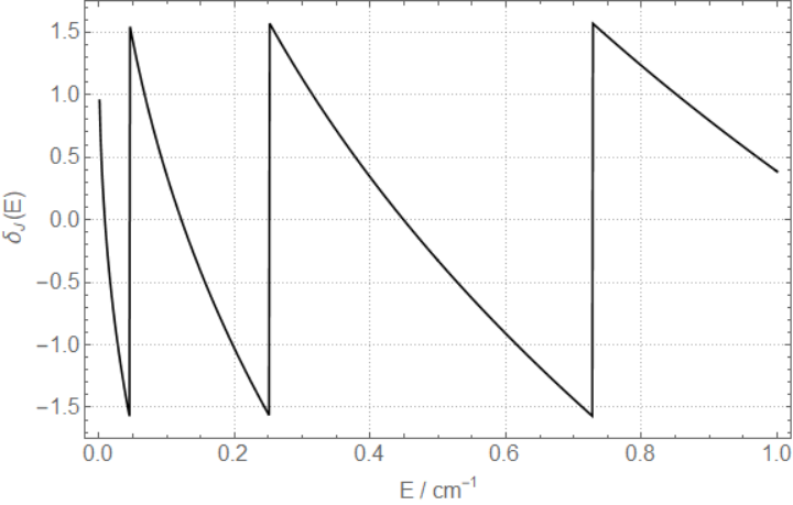
As a result of this definition, the eigenphase (in radians) is the same modulo . The eigenphases presented in this work are given in the range . This leads to seeming discontinuities, e.g. in Figure 5 when the eigenphase passes through . These discontinuities are characteristic of resonances which are also present in the eigenphases. Although the eigenphase is technically not a scattering observable itself, it can be used to construct the other three observables used in this work, and is consequently the best variable for the detection of resonances.
The total cross-section for an interaction can be given as the sum over partial waves from a minimum value to a maximum , . It is given by:
| (10) |
and the cross-section for a given partial wave, is merely the summand of Equation (10).
The scattering length, , and the effective range, , are numbers that characterise the properties of the PEC and the scattering process at low energy. They can be defined in terms of a linear expansion at low energy. If one plots for as a function of , then for sufficiently low energy the plot should be linear. In this case, and are defined in the following way:
| (11) |
ignoring higher order terms in .
Another observable it is possible to detect using the eigenphase is a resonance. A resonance will appear as a feature in a plot of the eigenphase or cross-section as a function of . Furthermore, the energy of the resonance, and its width – the inverse of its lifetime – can be determined by fitting a function to the eigenphase following the form of Breit and Wigner Breit and Wigner 1936; Burke 2011; Tennyson and Noble 1984:
| (12) |
where is the eigenphase for partial wave at scattering energy , is the width of the given resonance, and is the energy of the resonance. Note this definition of follows that in standard use in scattering (eg Tennyson and Noble 1984), and differs by factor of two from the definition a full width at half maximum (FWHM).
The non-resonant shape of the eigenphase (the ‘background’ eigenphase) is accounted for by the two terms and , where it is assumed that the width is narrow enough that the background eigenphase can be approximated by a linear function of over its length. By fitting a generated eigenphase to a function of this form, values for and can be obtained. Note that it is sometimes necessary to replace the final term in Equation (12) with its negative, if it is required by the resonance shape.
III Results
III.1 Bound states
When performing the inner region calculations with Duo in this work, the number of bound states was found to be in agreement with literature values Barletta et al. 2010; Sahraeian and Hadizadeh 2018 for all five PECs studied (see Table 1).
However, there were considerable complications when attempting to detect the ninth bound state in this work for the PECs where it was predicted to exist – the PS and PM potentials. As this state is so weakly bound, it was necessary to extend the inner region calculations out to large distances in order to detect it. This ninth bound state has many similarities to a halo state Owens and Špirko 2018, as seen in Figure 2, which shows the ninth bound state as a function of for the PM PEC for when Å.
The results in Table 3 of this work were obtained only by extending out to distances of over 35 Å for the PM PEC and over 40 Å for the PS PEC. As such, a very large number of points needed to be used in order to maintain precision. The difficulty in detecting the ninth bound state is underlined by the fact that when the diatomic nuclear motion code LEVEL Le Roy 2016 was used, the ninth bound state was never detected for any of PECs considered here, no matter how far out or how many points the inner region was integrated over. Sahraeian et al. Sahraeian and Hadizadeh 2018 also cited difficulties in detecting this state, which they quote a value of for.
Consequently the actual binding energy of the ninth bound state, for PECs in which it was detected, varied as a function of the used in the integration here, up to 100 Å. This is seen in Figure 3, which shows the value of the ninth bound state, , of the PM and PS PECs as a function of , for all values of under 105 Å for which the state was actually bound. If the calculations are converging on fixed values of , they are significantly different from the value obtained by Sahraeian et al.
Once a threshold value of was reached, every PEC that the literature claimed had nine bound states were consistently found to do so, even if its value changed with . No ninth bound state was detected in this work for any PEC for which it was claimed that there are only eight bound states, even when using large values of over 100 Å. More assessment of the numerical issues faced by the R-matrix method can be found in Rivlin et al. Rivlin et al. 2018.
We note that diffuse bound states whose wavefunctions extend significantly beyond can be found rather efficiently within an R-matrix formalism by performing scattering calculations with negative energies Sarpal et al. 1991; Little and Tennyson 2013. We plan to implement such a procedure within the RmatReact framework.
III.2 Resonances
The supplementary data provided by Myatt et al. Myatt et al. 2018 (MD) includes the rovibrational eigenenergies of the system obtained using LEVEL Le Roy 2016. The supplementary data also quotes values for states which lie above the dissociation threshold but below a centrifugal barrier for , known as quasibound states. The quasibound states from Myatt et al. Myatt et al. 2018 which have quantum numbers are quoted in Table 2.
|
|
|
|
|
| |||||||||||||
|---|---|---|---|---|---|---|---|---|---|---|---|---|---|---|---|---|---|---|
| 6 | 9 | 0.129 | 0.1287 | 0 | 0 | |||||||||||||
| 6 | 10 | 0.448 | 0.00330 | 0.4486(2) | 0.00247(46) | -0.107 | 0.757 | |||||||||||
| 7 | 5 | 0.071 | 0.00605 | 0.06993(5) | 0.004841(5) | 0.00213 | -0.997 |
In this work, the quasibound states quoted for the MD potential in Myatt et al. Myatt et al. 2018 were characterised by analysing resonances in the scattering calculation. The diatomic nuclear motion code used in this work, Duo, does not have the capacity to detect quasibound eigenvalues directly (although it is possible to detect them using a stabilisation method with continuum states). However, these quasibound states should correspond to shape resonances, which can be detected in plots of the eigenphase and cross-section.
In order to detect the shape resonances, the RmatReact method was used to generate the eigenphase, and from it the partial cross-sections for all the partial waves with . The inner region was calculated using 500 Lobatto grid points between Å and Å. The outer region propagation was performed from Å to Å, with over 1,000 propagation iterations.
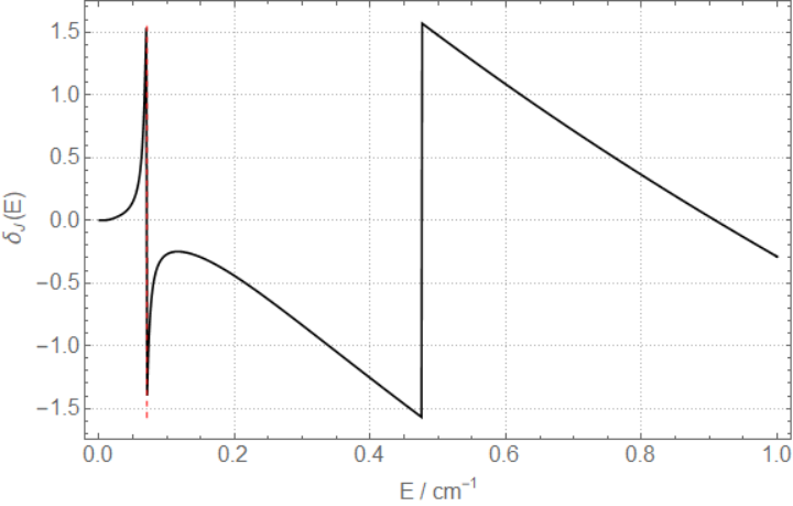
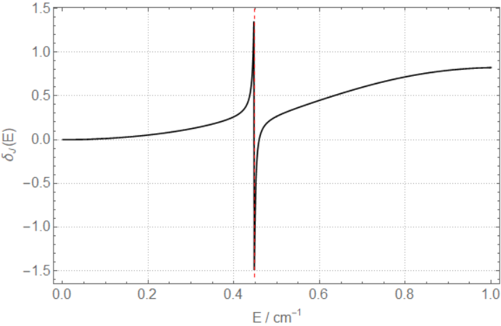
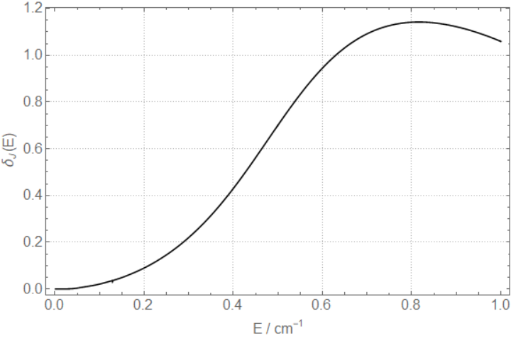
Figure 5 shows the eigenphase and cross-section generated using the MD potential for , , and . Figure 6 shows the eigenphase and cross-section generated using the MD potential for . In all these cases, the eigenphase and cross-section were calculated for energies between and .
The partial wave plots are included in Figure 5 to indicate what a typical eigenphase and cross-section looks like for this system when no resonances are present: in the cross-section plot the cross-section sharply rises at low energies.
Myatt et al. Myatt et al. 2018 predicted (see Table 2) that there should be quasibound states in the , , and partial waves. These resonances can clearly be seen in our calculations (Figures 5 and 6) where their positions are marked with dashed lines. These three states are the only quasibound states given by Myatt et al. for and the only resonances detected in this work.
For the and resonances, the energy , width , and and parameters were fitted to the Breit-Wigner form of Equation (12), using the values quoted by Myatt et al. as the starting point of the fitting procedure. The very narrow resonance could not be fit in this way, and so the energy location of the width was determined by identifying where the eigenphase suddenly went from to and identifying the two points either side of this jump; was taken as the mid-point between them. This energy was then inserted directly into the Breit-Wigner fit.
Figure 4 shows the result of this procedure for the resonance in the partial wave. The fitting was performed using the energy range to , using the Levenberg-Marquardt algorithm as implemented in the software Origin (OriginLab, Northhampton, MA).
Table 2 contains the results of this fitting procedure for all three resonances studied in this work (all using the same software and algorithm with appropriate energy ranges). The narrowest resonance is for and there is very good agreement between our results and those quoted by Myatt et al. Myatt et al. 2018. For the other two, broader resonances we find slightly different positions and widths. This is consistent with the full treatment of coupling to the continuum obtained in a scattering calculation: LEVEL, as used by Myatt et al. for their quasibound states, is known to be less well-adapted for characterising broader resonances Le Roy 2016; Doss et al. 2006. Both the resonance position and width for are also similar to the figures quoted by Čížek et al. Čížek and Horáček 1996.
As Figure 6 and Table 2 show, narrow resonances can be hard to detect. The only resonances detected in this work were ones which had been previously predicted and only needed to be corroborated. In the future, a more sophisticated resonance-detecting software such as those by Tennyson and Noble Tennyson and Noble 1984 or Noble et al. Noble et al. 1993, or possibly a procedure based on the complex analysis of the S-matrix Burke 2011 such as that of Čížek and Horáček Cízek and Horácek 1996, will be used to to detect resonances which may otherwise be missed.





Finally, Figure 7 shows the total cross-section generated using the RmatReact method with the MD potential. The quasibound states predicted by Myatt et al. Myatt et al. 2018 are also pictured. This figure gives a good overview of the properties of argon-argon scattering at low energy. It is notable for having many features. Besides the three resonances, there is also more structure to the plot – something that is more prevalent in heavy particle scattering than electron-atom or electron-molecule scattering due to the greater number of partial waves contributing to the scattering process. Furthermore, the cross-section tends to a large value at the lowest energies on the graph. This corroborates the feature seen in Figure 8 towards the lowest energies where the cross section becomes very large.
Thus far we have not considered the consequences of the Pauli principle. 40Ar is a Boson with zero nuclear spin; as a consequence collisions with odd are forbidden. Figure 7 shows the observable cross section obtained by simply summing partial waves with even . As a consequence the resonances with and disappear and there is a pronounced Ramsauer minimum at about 0.01 .

III.3 Low-energy Scattering
In order to analyse low-energy scattering behaviour, the cross-section for was plotted for to E = 1 on a log-log axis, see Figure 8. The same numerical parameters were used as in Section III.2. The plot shows that the cross-section tends towards a constant at lower energies, which is predicted by Equation (11).

Figure 9 analyses the region of validity of the low-energy linear fit of Equation (11). It is designed to re-create a plot shared as private communications by the authors of Ref. Barletta et al. 2010.
The solid, red line of Figure 9 represents the eigenphase calculation generated by the RmatReact method, using an R-matrix inner region ranging from Å to Å, an integration over 1600 Lobatto grid points, and an R-matrix propagation from Å to Å, with 1000 propagation iterations. The dashed line represents Equation (11), with the parameters and determined by using a least-squares linear fit of the lower-energy portion of the red line (intercept Å-1, slope Å), again using the software Origin. As with Table 3, this Figure is in agreement with results provided in private communications by Barletta et al. Barletta et al. 2010, who also computed the scattering length of the collision based on the potential due to Aziz Aziz 1993. It can be seen from Figure 9 that the plot is only linear at a very low energy.
A similar low-energy fitting procedure in Origin was performed for all five PECs studied. The values of and were calculated in this work for the four PECs where corresponding literature values could be obtained, the comparison of which can be seen in Table 3.
The effective ranges featured in Table 3 all appear to be in broad agreement. This is to be expected since this quantity is not especially sensitive to fine changes to the quantity of the potential, and is not affected significantly by the number of bound states Burke 2011.
The values obtained for the scattering length are found to be sensitive to the energy range used in the fitting procedure, and so whilst numbers are quoted in Table 3, it should be noted that these numbers are not intended to be definitive. When using the energy range of Figure 9 for the low-energy fit, it is possible to obtain the scattering lengths quoted in Barletta et al. 2010 to within a 5% relative difference. However, when using a much lower energy range for the fit of Å-2 to Å-2, the scattering lengths change significantly. (The effective ranges also change slightly, but are still in agreement.) The values quoted in Table 3 are the ones created using the lower energy range fit. As Figure 9 shows, this lower range is where the expansion of Equation(11) is most appropriate.
The features seen towards the right of Figure 8 correspond to energies where the eigenphase pass through zero. On a log-log plot of the cross-section these crossings manifest as the dips seen in the Figure.
Although the scattering length values diverge from each other very significantly, the RmatReact method was able to qualitatively corroborate each one. The PECs in Table 3 which have a negative scattering length correspond to PECs for which there are eight bound states in literature (see Table 1). The only PEC considered which supports nine bound states, PM Patkowski et al. 2005, has a large, positive scattering length.
This is in line with the observation that the scattering length is strongly affected by the energy of the highest bound state. If the scattering length is plotted as a function of , the minimum of the potential, then there is a pole at points where the number of bound states increments by one, going up to positive infinity in one direction and down to negative infinity in the other Burke 2011. That means that either side of this pole, the scattering length can be very different: any real number is a potentially valid scattering length.
| Potential |
|
|
|
| ||||||||
|---|---|---|---|---|---|---|---|---|---|---|---|---|
| Aziz Aziz 1993 | -505.6 | -647.1 | 35.94 | 35.53 | ||||||||
| PM Patkowski et al. 2005 | 1285 | 844.0 | 33.87 | 33.53 | ||||||||
| TT Tang and Toennies 2003 | -60.79 | -62.50 | 50.12 | 49.20 | ||||||||
| MD Myatt et al. 2018 | -714 | -709.3 | – | 35.41 |
It is known Faas et al. 2000; Patkowski et al. 2005 that relativistic and nonadiabatic effects can impact potential parameters such as the depth of the potential. The different PECs studied in this work all incorporate these effects to different degrees. Whilst this work attempts to verify the scattering observables produced using these potentials, no attempt is made to assess the quality of each potential relative to the other ones. These effects, along with the other sources of uncertainty related to the PECs, are by far the biggest source of uncertainty and error in the results, and contribute much larger error to the numbers quoted here than numerical errors in the algorithm itself.
No previous values are available for the scattering length and effective range of the PS PEC Patkowski and Szalewicz 2010; the scattering length and effective range were calculated, using the same lower energy range fitting as the results in Table 3. The scattering length was found to be 1669 Å to four significant figures. This is noteworthy because both this work and Sahraeian et al. Sahraeian and Hadizadeh 2018 claim to have detected nine bound states for this system, and so the PS PEC continues the pattern of large, positive scattering lengths for PECs with nine bound states, as seen in Table 3. Finally, the effective range was found to be 33.82 Å, in good agreement with most of the other effective ranges cited in the literature and this work.
IV Conclusions and outlook
In this paper the validity and accuracy of the RmatReact method for the single-channel, diatomic case was demonstrated by comparing results generated using it to other literature results. In doing so, the accuracy of the scattering length, and the positions of the resonances generated by Myatt et al. Myatt et al. 2018 were confirmed. Most of the widths of the resonances generated by Myatt et al. were also confirmed.
This paper corroborated the qualitative features of the highly divergent scattering lengths quoted in Barletta et al. Barletta et al. 2010. This has interesting implications for the study of the low-energy behaviour of the argon-argon scattering interaction – the debate over the scattering length remains unresolved. Novel experimental techniques such as those in Beyer and Merkt 2018 may help to resolve the dispute over the scattering length and the alleged ninth bound state.
Further study of the single-channel, atom-atom scattering problem is intended. A resonance finder will be useful for detecting any narrow resonances missed by other authors. The S-matrix can be used for this purpose, and also for the equally useful purpose of detecting weakly-bound bound states Burke 2011; Sarpal et al. 1991.
In resolving the numerical difficulties of adapting pre-existing codes to the ‘harness’ of the RmatReact method, this work paves the way for the study of more complex interactions with the method. Other follow-ups to this work will include a study of a multichannel collision between atoms, and collisions between an atom and a diatom.
Eventually the RmatReact method is intended to evolve into a method that can be applied to even more complex reactants and reactions, to resolve the many outstanding questions in the field of ultracold scattering. A formulation of the method for treating chemical reactions in three particle systems has recently been presented McKemmish and Tennyson 2019.
Acknowledgements
This project has received funding from the European Union’s Horizon 2020 research and innovation programme under the Marie Sklodowska-Curie grant agreement No 701962, and from the EPSRC under grants EP/M507970/1 and EP/R029342/1. We would also like to acknowledge the contributions of the late Professor Robert J. Le Roy, in this and many other works we have been involved in.
References
- Stuhl et al. (2014) B. K. Stuhl, M. T. Hummon, and J. Ye, Ann. Rev. Phys. Chem. 65, 501 (2014).
- Stuhl et al. (2012) B. K. Stuhl, M. T. Hummon, M. Yeo, G. Quemener, J. L. Bohn, and J. Ye, Nature 492, 396 (2012).
- Shuman et al. (2010) E. S. Shuman, J. F. Barry, and D. DeMille, Nature 467, 820 (2010).
- Zhelyazkova et al. (2014) V. Zhelyazkova, A. Cournol, T. E. Wall, A. Matsushima, J. J. Hudson, E. A. Hinds, M. R. Tarbutt, and B. E. Sauer, Phys. Rev. A 89, 053416 (2014).
- Molony et al. (2014) P. K. Molony, P. D. Gregory, Z. Ji, B. Lu, M. P. Köppinger, C. R. Le Sueur, C. L. Blackley, J. M. Hutson, and S. L. Cornish, Phys. Rev. Lett. 113, 255301 (2014).
- Dawid et al. (2018) A. Dawid, M. Lewenstein, and M. Tomza, Phys. Rev. A 97, 063618 (2018).
- Bohn (2001) J. L. Bohn, Phys. Rev. A 63, 052714 (2001).
- Köhler et al. (2006) T. Köhler, K. Góral, and P. S. Julienne, Rev. Mod. Phys. 78, 1311 (2006).
- Heazlewood and Softley (2015) B. R. Heazlewood and T. P. Softley, Ann. Rev. Phys. Chem. 66, 475 (2015).
- Bell and Softley (2009) M. T. Bell and T. P. Softley, Mol. Phys. 107, 99 (2009).
- Bell et al. (2009) M. T. Bell, A. D. Gingell, J. M. Oldham, T. P. Softley, and S. Willitsch, Faraday Disc. 142, 73 (2009).
- Quemener and Julienne (2012) G. Quemener and P. S. Julienne, Chem. Rev. 112, 4949 (2012).
- Ospelkaus et al. (2010) S. Ospelkaus, K.-K. Ni, D. Wang, M. H. G. De Miranda, B. Neyenhuis, G. Quéméner, P. S. Julienne, J. L. Bohn, D. S. Jin, and J. Ye, Science 327, 853 (2010).
- Chin et al. (2010) C. Chin, R. Grimm, P. Julienne, and E. Tiesinga, Rev. Mod. Phys. 82, 1225 (2010).
- Pellegrini et al. (2008) P. Pellegrini, M. Gacesa, and R. Côté, Phys. Rev. Lett. 101, 053201 (2008).
- Hutson et al. (2009) J. M. Hutson, M. Beyene, and M. L. González-Martínez, Phys. Rev. Lett. 103, 163201 (2009).
- D’Incao et al. (2004) J. P. D’Incao, H. Suno, and B. D. Esry, Phys. Rev. Lett. 93, 123201 (2004).
- Lompe et al. (2010) T. Lompe, T. B. Ottenstein, F. Serwane, A. N. Wenz, G. Zürn, and S. Jochim, Science 330, 940 (2010).
- Ferlaino et al. (2011) F. Ferlaino, A. Zenesini, M. Berninger, B. Huang, H.-C. Nägerl, and R. Grimm, Few-Body Systems 51, 113 (2011).
- Wang and Esry (2009) Y. Wang and B. D. Esry, Phys. Rev. Lett. 102, 133201 (2009).
- D’Incao and Esry (2006) J. P. D’Incao and B. D. Esry, Phys. Rev. A 73, 030703 (2006).
- Carrington et al. (1982) A. Carrington, J. Buttenshaw, and R. Kennedy, Mol. Phys. 45, 753 (1982).
- Henderson and Tennyson (1996) J. R. Henderson and J. Tennyson, Mol. Phys. 89, 953 (1996).
- Kemp et al. (2000) F. Kemp, C. Euan Kirk, and I. R. McNab, Phil. Trans. A 358, 2403 (2000).
- Tennyson et al. (2017) J. Tennyson, O. L. Polyansky, N. F. Zobov, A. Alijah, and A. G. Császár, J. Phys. B: At. Mol. Opt. Phys. 50, 232001 (2017).
- Mayle et al. (2013) M. Mayle, G. Quemener, B. P. Ruzic, and J. L. Bohn, Phys. Rev. A 87, 012709 (2013).
- Tennyson (2010) J. Tennyson, Phys. Rep. 491, 29 (2010).
- Burke (2011) P. G. Burke, R-Matrix Theory of Atomic Collisions: Application to Atomic, Molecular and Optical Processes, vol. 61 (Springer Science & Business Media, 2011).
- Bocchetta and Gerratt (1985) C. J. Bocchetta and J. Gerratt, J. Chem. Phys. 82, 1351 (1985).
- Light and Walker (1976) J. C. Light and R. B. Walker, J. Chem. Phys. 65, 4272 (1976).
- Walker and Light (1980) R. B. Walker and J. C. Light, Ann. Rev. Phys. Chem. 31, 401 (1980).
- Burke et al. (1998) J. P. Burke, C. H. Greene, and J. L. Bohn, Phys. Rev. Lett. 81, 3355 (1998).
- Raoult and Mies (2004) M. Raoult and F. H. Mies, Phys. Rev. A 70, 012710 (2004).
- Gao et al. (2005a) B. Gao, E. Tiesinga, C. J. Williams, and P. S. Julienne, Phys. Rev. A 72, 042719 (2005a).
- Croft et al. (2011) J. F. E. Croft, A. O. G. Wallis, J. M. Hutson, and P. S. Julienne, Phys. Rev. A 84, 042703 (2011).
- Croft et al. (2012) J. F. E. Croft, J. M. Hutson, and P. S. Julienne, Phys. Rev. A 86, 022711 (2012).
- Tennyson et al. (2016) J. Tennyson, L. K. McKemmish, and T. Rivlin, Faraday Discuss. 195, 31 (2016).
- Rivlin et al. (2018) T. Rivlin, L. K. McKemmish, and J. Tennyson, in Quantum Collisions and Confinement of Atomic and Molecular Species, and Photons, edited by P. C. Deshmukh, E. Krishnakumar, S. Fritzsche, M. Krishnamurthy, and S. Majumder (Springer, 2018), Springer Conference Series.
- Patkowski et al. (2005) K. Patkowski, G. Murdachaew, C. M. Fou, and K. Szalewicz, Mol. Phys. 103, 2031 (2005).
- Aziz (1993) R. A. Aziz, J. Chem. Phys. 99, 4518 (1993).
- Aziz and Chen (1977) R. A. Aziz and H. H. Chen, J. Chem. Phys. 67, 5719 (1977).
- Song et al. (2010) B. Song, X. Wang, J. Wu, and Z. Liu, Fluid Phase Equilibria 290, 55 (2010).
- Tang and Toennies (2003) K. T. Tang and J. P. Toennies, J. Chem. Phys. 118, 4976 (2003).
- Patkowski and Szalewicz (2010) K. Patkowski and K. Szalewicz, J. Chem. Phys. 133, 094304 (2010).
- Myatt et al. (2018) P. T. Myatt, A. K. Dham, P. Chandrasekhar, F. R. W. McCourt, and R. J. Le Roy, Mol. Phys. 116, 1 (2018).
- Edmunds and Barker (2014) P. D. Edmunds and P. F. Barker, Phys. Rev. Lett. 113, 183001 (2014).
- Barletta et al. (2010) P. Barletta, J. Tennyson, and P. F. Barker, New J. Phys 12, 113002 (2010).
- Barletta et al. (2009) P. Barletta, J. Tennyson, and P. F. Barker, New J. Phys 11, 055029 (2009).
- Slaví́ček et al. (2003) P. Slaví́ček, R. Kalus, P. Paška, I. Odvárková, P. Hobza, and A. Malijevskỳ, J. Chem. Phys. 119, 2102 (2003).
- Meshkov et al. (2011) V. V. Meshkov, A. V. Stolyarov, and R. J. Le Roy, J. Chem. Phys. 135, 154108 (2011).
- Sahraeian and Hadizadeh (2018) T. Sahraeian and M. R. Hadizadeh, Intern. J. Quantum Chem. p. e25807 (2018).
- Wigner (1946) E. P. Wigner, Phys. Rev. 70, 15 (1946).
- Wigner and Eisenbud (1947) E. P. Wigner and L. Eisenbud, Phys. Rev. 72, 29 (1947).
- Robson (1969) B. Robson, Nuclear Physics A 132, 5 (1969).
- Buttle (1967) P. Buttle, Phys. Rev. 160, 719 (1967).
- Baluja et al. (1982) K. Baluja, P. Burke, and L. Morgan, Comput. Phys. Commun. 27, 299 (1982).
- Burke and Schey (1962) P. G. Burke and H. M. Schey, Phys. Rev. 126, 147 (1962).
- Gailitis (1976) M. Gailitis, J. Phys.B: At. Mol. Phys. 9, 843 (1976).
- Gao (2001) B. Gao, Physical Review A 64, 010701 (2001).
- Gao et al. (2005b) B. Gao, E. Tiesinga, C. J. Williams, and P. S. Julienne, Physical Review A 72, 042719 (2005b).
- Yurchenko et al. (2016) S. N. Yurchenko, L. Lodi, J. Tennyson, and A. V. Stolyarov, Comput. Phys. Commun. 202, 262 (2016).
- Lill et al. (1982) J. Lill, G. Parker, and J. Light, Chemical Physics Letters 89, 483 (1982).
- Light et al. (1985) J. Light, I. Hamilton, and J. Lill, J. Chem. Phys. 82, 1400 (1985).
- Manolopoulos (1993) D. Manolopoulos, in Numerical Grid Methods and Their Application to Schrödinger’s Equation (Springer, 1993), pp. 57–68.
- Manolopoulos and Wyatt (1988) D. Manolopoulos and R. Wyatt, Chem. Phys. Lett. 152, 23 (1988).
- Meyer (1994) H.-D. Meyer, Chemical physics letters 223, 465 (1994).
- Manolopoulos and Wyatt (1989) D. Manolopoulos and R. Wyatt, Chemical Physics Letters 159, 123 (1989).
- Colbert and Miller (1992) D. T. Colbert and W. H. Miller, J. Chem. Phys. 96, 1982 (1992).
- Zvijac and Light (1976) D. J. Zvijac and J. C. Light, Chem. Phys. 12, 237 (1976).
- Schneider and Walker (1979) B. I. Schneider and R. B. Walker, J. Chem. Phys. 70, 2466 (1979).
- Sunderland et al. (2002) A. G. Sunderland, C. J. Noble, V. M. Burke, and P. G. Burke, Comput. Phys. Commun. 145, 311 (2002).
- Gradshteyn and Ryzhik (2014) I. S. Gradshteyn and I. M. Ryzhik, Table of integrals, series, and products (Academic press, 2014).
- Breit and Wigner (1936) G. Breit and E. Wigner, Phys. Rev. 49, 519 (1936).
- Tennyson and Noble (1984) J. Tennyson and C. J. Noble, Comput. Phys. Commun. 33, 421 (1984).
- Owens and Špirko (2018) A. Owens and V. Špirko, Journal of Physics B: Atomic, Molecular and Optical Physics 52, 025102 (2018).
- Le Roy (2016) R. J. Le Roy, J. Quant. Spectrosc. Radiat. Transf. (2016).
- Sarpal et al. (1991) B. K. Sarpal, S. E. Branchett, J. Tennyson, and L. A. Morgan, J. Phys. B: At. Mol. Opt. Phys. 24, 3685 (1991).
- Little and Tennyson (2013) D. A. Little and J. Tennyson, J. Phys. B: At. Mol. Opt. Phys. 46, 145102 (2013).
- Doss et al. (2006) N. Doss, J. Tennyson, A. Saenz, and S. Jonsell, Phys. Rev. C 73, 025502 (2006).
- Čížek and Horáček (1996) M. Čížek and J. Horáček, Czech. J.Phys. 46, 55 (1996).
- Noble et al. (1993) C. Noble, M. Dorr, and P. Burke, J. Phys. B: At. Mol. Opt. Phys. 26, 2983 (1993).
- Cízek and Horácek (1996) M. Cízek and J. Horácek, J. Phys. A: Math. Gen. 29, 6325 (1996).
- Fano (1961) U. Fano, Physical Review 124, 1866 (1961).
- Faas et al. (2000) S. Faas, J. Van Lenthe, and J. Snijders, Molecular Physics 98, 1467 (2000).
- Beyer and Merkt (2018) M. Beyer and F. Merkt, Physical Review X 8, 031085 (2018).
- McKemmish and Tennyson (2019) L. K. McKemmish and J. Tennyson, Phil. Trans. Royal Soc. London A (2019).