AutoSF: Searching Scoring Functions for Knowledge Graph Embedding
Abstract
Scoring functions (SFs), which measure the plausibility of triplets in knowledge graph (KG), have become the crux of KG embedding. Lots of SFs, which target at capturing different kinds of relations in KGs, have been designed by humans in recent years. However, as relations can exhibit complex patterns that are hard to infer before training, none of them can consistently perform better than others on existing benchmark data sets. In this paper, inspired by the recent success of automated machine learning (AutoML), we propose to automatically design SFs (AutoSF) for distinct KGs by the AutoML techniques. However, it is non-trivial to explore domain-specific information here to make AutoSF efficient and effective. We firstly identify a unified representation over popularly used SFs, which helps to set up a search space for AutoSF. Then, we propose a greedy algorithm to search in such a space efficiently. The algorithm is further sped up by a filter and a predictor, which can avoid repeatedly training SFs with same expressive ability and help removing bad candidates during the search before model training. Finally, we perform extensive experiments on benchmark data sets. Results on link prediction and triplets classification show that the searched SFs by AutoSF, are KG dependent, new to the literature, and outperform the state-of-the-art SFs designed by humans.
I Introduction
Knowledge Graph (KG) [33, 28, 40], as a special kind of graph structure with entities as nodes and relations as edges, is important to both data mining and machine learning, and has inspired various downstream applications, e.g., structured search [33, 7, 36], question answering [25] and recommendation [52]. In KGs, each edge is represented as a triplet with form (head entity, relation, tail entity), denoted as . A fundamental issue is how to quantize the plausibility of triplets s [14, 40]. KG embedding (KGE) has recently emerged and been developed as a promising method serving this purpose [30, 46, 29, 6, 39, 24, 18, 19, 54]. Basically, given a set of observed triplets, KGE attempts to learn low-dimensional vector representations of entities and relations so that the plausibility of triplets can be quantized. Scoring function (SF), which returns a score for based on the embeddings, is used to measure the plausibility. Generally, SF is designed and chosen by humans and it has significant effects on embeddings’ quality [28, 40, 20].
Ever since the invention of KGE, many SFs have been proposed in the literature. Let the embedded vectors of , and be , and respectively. TransE [4], a representative embedding model, interprets the triplet as a translation from head entity to tail entity , i.e. the embeddings satisfy . Variants of TransE like TransH [43] and TransR [21], project the embedding vector into different spaces and enables the embedding to model relationships that are one-to-many, many-to-one or many-to-many. These models are categorized into translational distance models (TDMs). However, as proved in [41, 42], TDMs are not fully expressive and their empirical performance is inferior to other models. RESCAL [30], DistMult [46], ComplEx [39], Analogy [24] and more recently proposed SimplE [18, 19], use a bilinear function to model the plausibility of triplets, where is a square matrix related to relation embedding. These models belong to the bilinear model (BLMs). Different BLMs use different constrains to regularize the relation matrix in order to adapt to different datasets. Inspired by the success of deep networks [2], some neural network models (NNMs) have also been explored as SFs, e.g., MLP [7], NTM [34], Neural LP [47] and ConvE [6]. Even though neural networks are powerful and have strong expressive ability, the NNMs do not perform well in KGE domain because of not being well-regularized.
Among the existing SFs, BLM-based ones are the most powerful as indicated by both the state-of-the-art results [19] and theoretical guarantees on expressiveness [41, 18]. However, since different KGs have distinct patterns in relations [32], a SF which adapts well to one KG may not perform consistently well on other KGs. Besides, designing new SFs to outperform state-of-the-art SFs is challenging. Therefore, how to choose and design a good SF for a certain KG is a non-trivial and difficult problem.
Recently, automated machine learning (AutoML) [50, 17] has exhibited its power in many machine learning tasks and applications, e.g. model selection [13], image classification [23, 51] and recommendation [48]. In order to select proper models and hyper-parameters for different tasks, hyperparameter optimization (HPO) has been proposed [13, 11] to effectively and efficiently find better configurations, which previously requires great human efforts. Another hot trend in AutoML is to search better neural networks for deep learning models. Neural architecture search (NAS) [55] has identified networks with fewer parameters and better performance than networks designed by humans.
Inspired by the success of AutoML, we aim to design better and novel data-dependent SFs for KGE. Specifically, we propose automated scoring function (AutoSF) which can automatically search an SF for a given KG. It can not only reduce human’s effort in designing new SFs, but also make adaptation to different KGs. However, it is not easy to achieve the above goal. When applying AutoML, two important perspectives, i.e. search space, which helps to figure out important properties of the underling problems, and search algorithm, which determines the efficiency of finding better points in the space, need serious consideration. In this work, we have made the following contributions to achieve the goals:
- •
First, we make an important observation over existing SFs, which allows us to represent the BLM-based SFs in a unified form. Based on the unified representation, we formulate the design of SFs as an AutoML problem (i.e. AutoSF), and set up the corresponding search space. The space is not only specific enough to cover good SFs designed by humans, but also general enough to include novel SFs not visited in the literature.
- •
Second, we observe it is common that different KGs have distinct properties on relations that are symmetric, asymmetric, inverse, etc. This inspires us to conduct domain-specific analysis on the KGE models, and design constraints to effectively guide subsequent searches in the space.
- •
Third, we propose a progressive greedy algorithm to search through such a space. We further build a filter to avoid training redundant SFs and a predictor with specifically designed symmetry-related features (SRF) to select promising SFs. The search algorithm can significantly reduce the search space size by capturing the domain specific properties of candidate SFs.
- •
Finally, experimental results on five popular benchmarks on link prediction and triplet classification tasks demonstrate that the SFs searched by AutoSF outperform the start-of-the-art SFs designed by humans. In addition, the searched SFs are KG dependent and new to the literature. We further conduct case study on the searched SFs to provide means for analyzing KGs, which can inspire better understanding of embedding techniques for future researches.
Notations. We denote vectors by lowercase boldface, and matrix by uppercase boldface. A KG contains a set of triplets with and , where and are the set of entities and relations, respectively. For simplicity, the embeddings are represented by letters of indices in boldface, e.g. , , are embeddings of , respectively, and share the same set of embedding parameters . is the triple dot product and can be alternatively represented as , where is the diagonal matrix of . We denote the complex vector with . The conjugate of a complex vector is .
II Related Works
II-A Knowledge graph embedding (KGE)
| scoring function | embeddings | definition | relation types that can model |
|---|---|---|---|
| DistMult [46] | symmetric | symmetric | |
| ComplEx [39] / HolE [29] | Re | symmetric, anti-symmetric, asymmetric, inverse | |
| Analogy [24] | , | + Re | symmetric, anti-symmetric, asymmetric, inverse |
| SimplE [18] / CP [19] | , | + | symmetric, anti-symmetric, asymmetric, inverse |
Given a set of observed (positive) triplets, the goal of KGE is to learn low-dimensional vector representations of entities and relations so that the plausibility measured by of observed triplets s are maximized while those of non-observed ones are minimized [40]. To build a KGE model, the most important thing is to design and choose a proper SF , which measures the triplets’ plausibility based on embeddings. Since different SFs have different strengths and weaknesses, the choice of is critical for the KGE’s performance [40, 20]. A large amount of KGE models with popular SFs follow the same framework (Alg.1) [40] using stochastic gradient descent. At step 5, negative triplets are sampled from , which contains all non-observed triplets for a current positive triplet , by some fixed distributions [43] or dynamic sampling schemes [54]. Next, the gradients are computed based on the given SF and embeddings, and are used to update the model parameters (step 6). Hinge loss [4] and logistic loss [46] are popularly used as . In this paper, we use the multi-class loss [19] since it currently achieves the best performance and has little variance.
Existing human-designed SFs mainly fall into three types:
- •
Translational distance models (TDMs): The translational approach exploits the distance-based SFs. Inspired by the word analogy results in word embeddings [2], the plausibility is measured based on the distance between two entities, after a translation carried out by the relation. In TransE [4], the SF is defined by the (negative) distance between and , i.e. . Other TDMs-based SFs, e.g., TransH [43], TransR [12], enhance over TransE by introducing extra mapping matrices.
- •
BiLinear models (BLMs): SFs in this group exploit the plausibility of a triplet by the product-based similarity. Generally, they share the form as where is a matrix referring to the embedding of relation [40, 41]. RESCAL [30] models the embedding of each relation by directly using . DistMult [46] overcomes the overfitting problem of RESCAL by constraining to be diagonal. ComplEx [39] allows and to be complex values, which enables handling asymmetric relations. HolE [29] uses a circular correlation to replace the dot product operation, but is proven to be equivalent to ComplEx [16]. Other variants like Analogy [24], SimplE [18] regularize the matrix in different ways.
- •
Neural network models (NNMs): Neural models aim to output the probability of the triplets based on neural networks which take the entities’ and relations’ embeddings as inputs. MLP proposed in [7] and NTN proposed in [34] are representative neural models. Both of them use a large amount of parameters to combine entities’ and relations’ embeddings. ConvE [6] takes advantage of convolutional neural network to increase the interaction among different dimensions of the embeddings.
As proved in [41], TDMs have less expressive ability than BLMs, which further leads to their inferior empirical performance. Based on the power of deep networks, NNMs are also introduced for KGE. However, due to the huge model complexity and increasing difficulty of training, as well as the lack of domain-specific constraints, their performance is still worse than BLMs [6, 19]. Therefore, we focus on BLMs in the sequel. The most representative BLMs are listed in Tab. I.
II-B Automated machine learning (AutoML)
Automated machine learning (AutoML) [17, 50] has recently exhibited its power in easing the usage of and designing better machine learning models. Basically, AutoML can be regarded as a bi-level optimization problem where we need to update model parameters by the training data sets and tune hyper-parameters by the validation data sets. Regarding the success of AutoML, there are two important perspectives:
- •
Search space: This helps to figure out important properties of the underlying learning models and set up the search space for an AutoML problem. First, the space needs to be general enough to cover human wisdom as special cases. However, the space cannot be too general, otherwise searching in the space will be too expensive.
- •
Search algorithm: Unlike convex optimization, there is no universal and efficient optimization tools. Once the search space is determined, efficient algorithms should be developed to search good points in the space.
We take NAS and HPO as examples. The search space in NAS is spanned by network operations, e.g., convolution with different sizes, skip-connections. Various tailor-made algorithms, such as reinforcement learning [55], evolution algorithms [44], and one-shot algorithms [23, 51], have been proposed for efficient optimization. For HPO, Bayesian optimization [13, 11] is usually customized to search the space made up by the hyper-parameters of the learning tools.
This paper is the first step towards automated embedding of knowledge graphs. However, such a step is not trivial since previous AutoML methods used in NAS and HPO cannot be directly applied to KGE. The main problem is that we need to explore domain-specific properties in defining the search space and designing efficient search algorithm to achieve effectiveness with less cost.



III The Search Problem
As mentioned in Sec.II, new designs of SFs have continuously boosted the performance of KGEs in recent years. However, there is no absolute winner among the human-designed SFs. Besides, as different KGs usually exhibit distinct patterns in relations, how to choose a proper SF to achieve good performance is non-trivial. These raise one question: can we automatically design a SF for a given KG with good performance guarantee? In this part, we define AutoSF as a searching problem and make deep analysis on the search space based on KG properties to address the question.
III-A AutoSF: Searching for SFs
Since SF is the crux to KGE and different KG has distinct properties, we are motivated to form the problem of designing new and better SFs as a searching problem. Specifically, we define it as follows:
Definition 1 (AutoML Problem).
Let be a KGE model (with indexed embeddings and structure ), measures the performance (the higher the better) of a KGE model on a set of triplets . The problem of searching the SF is formulated as:
| (1) | ||||
| s.t. | (2) |
where contains all possible choices of , and denote training and validation data sets.
Same as NAS [44, 55] and HPO [13, 11], AutoSF is formulated as a bi-level optimization problem. We firstly need to train the model to obtain (converged model parameters) on the training set by (2), and then search for a better which is measured by the performance on the validation set by (1). However, in this sequel we can see the search space of and search strategy in AutoSF are fundamentally different from previous AutoML works. They are closely related to KGE’s domain and new to the AutoML literature.
III-B Search space: a unified representation of BLM SFs
To solve the AutoSF problem, the first question is: what is a good search space ? As discussed in Sec.II-B, the space can neither be too specific nor too general. To motivate a good search space, let us look at some commonly used SFs (Tab. I) and dig out what are important properties of .
As discussed in Sec.II-A, the state-of-the-art performance of KGE models is achieved by BLMs [19, 18], thus we limit our scope to them. RESCAL [30] is not considered since it does not have good scalability [24, 39] and neither empirically perform well. The other models in Tab. I regularize the number of trainable parameters of square matrix to be the same as entity embedding dimensions. Therefore, we constrain the relation embedding size to be the same as the entity’s and learn different ways of mapping the relation embedding into a square matrix . Besides, as the summary of relation types in Tab. I, important properties are symmetric, anti-symmetric, asymmetric and inverse. These are important properties of good SFs. Thus, a search space should be able to handle the symmetric related properties. In addition, as will be discussed in Remark III.1, different SFs in BLMs differ in their way of regularizing the square matrix . Therefore, we are motivated to adaptively search how to regularize the relational matrix on different KGs.
To motivate such a space, we can see that there are two main differences among these SFs.
- •
The embedding can be either real or complex, e.g. DistMult v.s. ComplEx.
- •
When embedding vectors are split, different SFs combine them in distinct manners, e.g., Analogy v.s. SimplE.
| common relations | requirements on | requirements on | examples from WN18/FB15K |
|---|---|---|---|
| symmetric [46] | IsSimilarTo, Spouse | ||
| anti-symmetric [39, 29] | LargerThan, Hypernym | ||
| general asymmetric [24] | LocatedIn, Profession | ||
| inverse [18] | Hypernym, Hyponym |
III-B1 Dealing with complex embeddings
A complex vector with is composed of a real part and an imaginary part . To deal with the complex embeddings, we can use -dimensional real vector to represent the -dimensional complex vector [39, 1]. Let the complex embedding , where (same for ), then ComplEx can be expressed as
| (3) |
Similarly, DistMult [46] with -dimensional embeddings can also be denoted by and represented as two parts
| (4) |
III-B2 Dealing with different splits
To make the training parameters consistent, we also use -dimensional real valued embeddings to represent Analogy and SimplE. As given in Tab. I, embeddings in Analogy [24] are split into a real part , and a complex part , which can be denoted as a concatenated real vector in the similar way as ComplEx. And the SF is split as
| (5) |
In SimplE [18], two independent embedding vectors and are used to represent each entity and relation. The resulting SF becomes
| (6) |
III-B3 The unified representation
In order to deal with the two different partitions, i.e. ComplEx v.s. DistMult and Analogy v.s. SimplE, we split embedding as (same for and ) to cover (3), (4), (5) and (6). Note that any splits (with and is even) can be used to cover the SFs in Tab. I. We take in order to ensure a tractable search space. The transformation of each SF is then summarized as:
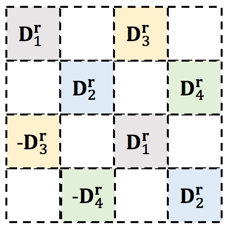
Based on above formulations, all the scoring functions can be formed as . Let for ,,,, the forms of for these SFs can be graphically represented as Fig. 1. In this way, we can see that the main difference between the four SFs is their way of filling the block matrix (see Fig. 1(e)). Based on such a pattern, we identify the search space of BLM-based SFs in Definition 2.
Definition 2 (Search space ).
Let return a block matrix, of which the elements in each block is given by where for . Then, SFs can be represented by
Remark III.1 (Searching to regularize BLMs).
Note that the SFs shown in Fig. 5 constrain the relation matrix in different forms, which can be regarded as different regularization schemes. Viewed in this way, AutoSF aims to search how to regularize the relational matrix that can adapt to different relation properties in different KGs. In addition, the data dependent regularization cannot be easily formed as a constraint in training procedure, which motivates us to use AutoML to search based on validation sets performance.
Remark III.2 (General Search Space).
Due to the recent success of deep networks [15] and the approximation ability of multilayer perceptron (MLP) [5], one may want to use a MLP as for (2). However, the design of the MLP is also a searching problem, which is very time-consuming [55]. Besides, an arbitrarily large MLP will lead to an extremely large space. As verified in [49], the general approximator MLP is a bad choice for NAS and performs worse than those using reinforcement learning [55].
IV The Search Strategy
Here, we propose an efficient search strategy to address the AutoSF problem based on domain-specific properties in KGs.
IV-A Challenges in algorithm design
Same as the other AutoML problems, the search problem of AutoSF is black-box, the search space is huge, and each step in the search is very expensive since both model training and evaluation should be involved. These problems have previously been touched by algorithms such as reinforcement learning [55], Bayes optimization [13] and genetic programming [44]. However, they are not a good choice here since we have domain-specific problems, i.e. expressiveness and invariance, in KGE, which are more challenging.
IV-A1 Expressiveness
It is clear that not all SFs (from Definition 2) are equally good. Expressiveness (Definition 3), which means should be better able to handle common relations in KGs , is of big concern for SFs. Their consequent requirements on and are summarized in Tab. II.
Definition 3 (Expressiveness [39, 18, 41]).
If can handle symmetric, anti-symmetric, general asymmetric, and inverse relations, then is expressive.


To ensure that can handle those common relations, we propose Proposition 1.
Proposition 1.
If can be symmetric for some , i.e. , and skew-symmetric for some , i.e. . Then the formulated is expressive. (Proofs in Appendix -A).
With this Proposition and to avoid trivial solutions, we introduce the following constraints on :
- (C1).
can be symmetric with proper and skew-symmetric with proper .
- (C2).
has no zero rows/columns, covers all to , and has no repeated rows/columns.
For (C1), the symmetric property of determines what kind of relation the given SF can model based on Proposition 1. For (C2), if there are zero rows/columns in , the corresponding embedding dimensions will be useless. It means that these dimensions will never be optimized during training.
The above constraints are important for finding potentially good candidate , and they play a key role in filtering out the bad ’s for the design of an efficient search algorithm. As in Definition 3 and Proposition 1, we need to deal with Constraint (C1) for expressiveness. It is challenging since only represents a structure, however the exact check of (C1) relies on the values in , which are unknown in advance. Fortunately, we can check it by value assignment. Take the SF in Fig. 2(a) for example. We can see that can be symmetric by assigning and as in Fig. 2(b), and skew-symmetric by setting and like in Fig. 2(c). This is the key idea of addressing expressiveness.
IV-A2 Invariance
As defined in Sec.III-B, the embeddings are split into 4 parts, i.e. . Prior to the embedding training, permuting the ’s will lead to equivalent structure since“1,2,3,4” here are only identity of each component and these components are equivalent at this stage. For example, we can permute into . Even though and change their position, the learned embedding could be the same by changing corresponding values after training. Therefore, the structure of SFs is invariance to permutation of ’s. Similarly, since and share the same embedding parameters , the generated SFs are also equivalent by simultaneously permuting the ’s and ’s. Moreover, if we flip the signs of some , we can learn equal embeddings by flipping the true value of those after training. In summary, there exist three kinds of invariance: permuting entity embedding ’s and ’s, permuting relation embedding ’s, and flipping signs. The example of three cases are given in Fig. 2(d-f). Let be the embeddings of the SF and be the embedding of another SF , and is formed through the invariance changes of . Then we will have after the model training. Therefore, it is tedious to train and evaluate the equivalents once we know the performance of one SF among them.
IV-B Progressive greedy search
As in Sec.III-B, adding one more block into indicates adding one more nonzero multiplicative term into , namely
| (7) |
where and . In order to search efficiently, we propose a progressive greedy algorithm based on the inductive rule (7), which can significantly cut down the search space in a stage-wise manner. The intuition of using (7) to progressively generate SFs it to gradually adjust the relation matrix . However, greedy search usually leads to sub-optimal solutions [38], which can be more serious when faced with the expressive and invariance challenges in AutoSF. Therefore, we enhance the greedy search with a filter and a predictor to specifically deal with the expressiveness and invariance discussed in Sec.IV-A.
IV-B1 Complete procedures
Alg.2 shows our progressive greedy algorithm. As in Definition 2, let the number of nonzero blocks in be and the SF in this group be . The idea of progressive search is that given the desired , we start from small blocks and then gradually add in more blocks until . Thus, we can greedily generate candidates based on the top SFs in at step 2-6 to reduce search space. Specifically, we greedily pick up the top- in the previously evaluated models in . candidates will then be generated by adding two more multiplicative term in step 4 to deal with Constraint (C1) since adding one block each step will result in simply lying on the diagonal. All the candidates are generated from and are checked through the Filter (see Sec.IV-B2) to guarantee Constraint (C2) and avoid training equivalents. Next, we use the predictor (see Sec.IV-B3) to further select promising candidates, which will then be trained and evaluated using Alg.1, in step 7 of Alg.2. The training data for is gradually collected with the trained SFs in at step 10.
IV-B2 Invariance - Using a filter
The filter we used in Alg.2 has two functions: 1) deal with Constraint (C2) and 2) remove equivalent structures due to invariance. Constraint (C2) is easy to check, given the structure of , we can directly map it into a substitute matrix and use to represent . Then checking requirements in (C2) is a trivial task, i.e. checking if the substitute matrix satisfies the Constraint (C2).
For the invariance, once a candidate fulfilling Constraint (C2) is generated, we use the invariance property to generate a set of equivalents . Specifically, we can permute the entity parts, relation parts, or flip signs to get equivalents of . If , we throw away since there are equivalent structures in the sampled set and history record . This step can dramatically help us to reduce the cost in training equivalent structures. Take as an example, the whole space is reduced from to 5 through the filter, namely there are only five good and unique candidates in . Besides, we add exception for the condition in step 5 of Alg.2 for since the number of candidates is smaller than .
IV-B3 Expressiveness - Constructing a predictor
Even though the filter helps to throw away many unpromising candidates, it does not deal with Constraint (C1). Hence, after collecting candidates, we use the predictor to further select promising ones among them. Considering that the performance of SFs on a specific KG is closely related to how the SF is formed, we can use a learning model, i.e. the predictor to predict the performance and select good candidates in advance. In general, we need to extract features for points which have been visited by the search algorithm, and then use a learning model to predict validation performance based on those features [13, 22]. The following are principles a good predictor needs to meet
- (P1).
Correlate well with true performance: the predictor needs not to accurately predict the exact values of validation performance, instead it should rank good candidates over bad ones;
- (P2).
Learn from small samples: as the real performance of each point in the search space is expensive to acquire, the complexity of the predictor should be low so that it can learn from few samples.
Based on Principle (P1), the extracted features from should be closely related to the quality of defined SF. Meanwhile, the features should be cheap to construct, i.e. they should not depend on values of , which are unknown before training. For (P2), the number of features should be small to guarantee a simple predictor. Therefore, we are motivated to design the symmetry-related features (SRFs), which can effectively capture to what extent can be symmetric or skew-symmetric (Proposition 2), and has low complexity.
Similar as the filter, we also use a substitute matrix to represent . As in Fig. 3, we use to represent , then the symmetric and skew-symmetric property of can be checked through and . Since is a simple matrix, the checking procedure is very cheap. Then by assigning different values to (details in Appendix -C), a 22-dimensional SRF will be returned. Considering that the correlation of SRFs with SFs’ performance is guaranteed under Proposition 2, we can use a simple two-layer MLP (22-2-1) as the predictor . Other regression models with low complexity may also work here.

Proposition 2.
The extracted SRFs (see Appendix -C) are (i) invariant to both the permutations and flipping signs of blocks in and (ii) give predictions related to symmetric or anti-symmetric properties.
IV-C Search complexity analysis
There are 16 blocks and each can be filled with 9 different contents , , , , . Thus the whole space size is , which is extremely large. The greedy strategy, predictor and filter cut down the space in different perspectives. Specifically, in each greedy step:
- •
Greedy: Considering that is progressively generated on for , there can be candidates ( is to choose location, is for the two s and is for signs). In comparison, there can be possible SFs in . Take for example, there are possible candidates. Since is generated based on the 5 good candidates in , we reduce the space size from to approximately based on the greedy scheme.
- •
Filter: The filter we designed is mainly used to deal with invariance properties. Permuting ’s leads to equivalent structures. Simultaneously permuting ’s and ’s also gives 24 equivalents. Besides, there are possible signs patterns. Therefore, given a , we can generate at most (there may exist same structures in this set) equivalent SFs, which should perform the same. Besides, by constraining the SF under Constraint (C2), many bad candidates can also be filtered out. Take as an example, only 5 candidates are selected to be trained among approximately possible structures.
- •
Predictor: Once candidates are generated, the predictor will select ones based on their predicted performance. Thus, the reducing ratio of predictor is about .
While it is difficult to directly quantize to which extend the three steps together can help to reduce the search space, we can observe the significance of efficiency gained through each component. Besides, we perform an empirical study in Sec.V-E to show the performance gaining of these steps.
| data set | #entity | #relation | #train | #valid | #test | #sym | #anti-sym | #inverse | #general |
|---|---|---|---|---|---|---|---|---|---|
| WN18 [4] | 40,943 | 18 | 141,442 | 5,000 | 5,000 | 4 | 7 | 7 | 0 |
| FB15k [4] | 14,951 | 1,345 | 484,142 | 50,000 | 59,071 | 66 | 38 | 556 | 685 |
| WN18RR [6] | 40,943 | 11 | 86,835 | 3,034 | 3,134 | 4 | 3 | 1 | 3 |
| FB15k237 [37] | 14,541 | 237 | 272,115 | 17,535 | 20,466 | 33 | 5 | 20 | 179 |
| YAGO3-10 [26] | 123,188 | 37 | 1,079,040 | 5,000 | 5,000 | 8 | 0 | 1 | 28 |
IV-D Comparison with existing AutoML approaches
The most related work in the AutoML literature is PNAS [22], which combines a greedy algorithm with a performance predictor to search a cell structure for the convolutional neural network (CNN). However, the filter is not used in PNAS as the search space for AutoSF is fundamentally different from that of CNN. Besides, PNAS adopts direct one-hot encoding for the predictor, which has a bad empirical performance here (see Sec.V-E1). As for the other AutoML approaches, even though the search problem of AutoSF is similarly defined as HPO [3, 9] and NAS [10], the search space and search algorithm of AutoSF are novel and specifically designed for KGE. There is no direct way for them to deal with the challenges in Sec.IV-A.
| WN18 | FB15k | WN18RR | FB15k237 | YAGO3-10 | ||||||||||||
| type | model | MRR | H@1 | H@10 | MRR | H@1 | H@10 | MRR | H@1 | H@10 | MRR | H@1 | H@10 | MRR | H@1 | H@10 |
| TDM | TransE [54] | 0.500 | — | 94.1 | 0.495 | — | 77.4 | 0.178 | — | 45.1 | 0.256 | — | 41.9 | — | — | — |
| TransH [54] | 0.521 | — | 94.5 | 0.452 | — | 76.6 | 0.186 | — | 45.1 | 0.233 | — | 40.1 | — | — | — | |
| RotatE [35] | 0.949 | 94.4 | 95.9 | 0.797 | 74.6 | 88.4 | 0.476 | 42.8 | 57.1 | 0.338 | 24.1 | 53.3 | — | — | — | |
| NNM | NTN [46] | 0.53 | — | 66.1 | 0.25 | 41.4 | — | — | — | — | — | — | — | — | — | |
| Neural LP [47] | 0.94 | — | 94.5 | 0.76 | — | 83.7 | — | — | — | 0.24 | — | 36.2 | — | — | — | |
| ConvE [6] | 0.942 | 93.5 | 95.5 | 0.745 | 67.0 | 87.3 | 0.46 | 39. | 48. | 0.316 | 23.9 | 49.1 | 0.52 | 45. | 66. | |
| BLM | TuckER [1] | 0.953 | 94.9 | 95.8 | 0.795 | 74.1 | 89.2 | 0.470 | 44.3 | 52.6 | 0.358 | 26.6 | 54.4 | — | — | — |
| HolEX [45] | 0.938 | 93.0 | 94.9 | 0.800 | 75.0 | 88.6 | — | — | — | — | — | — | — | — | — | |
| QuatE [53] | 0.950 | 94.5 | 95.9 | 0.782 | 71.1 | 90.0 | 0.488 | 43.8 | 58.2 | 0.348 | 24.8 | 55.0 | — | — | — | |
| DistMult | 0.821 | 71.7 | 95.2 | 0.817 | 77.7 | 89.5 | 0.443 | 40.4 | 50.7 | 0.349 | 25.7 | 53.7 | 0.552 | 47.6 | 69.4 | |
| ComplEx | 0.951 | 94.5 | 95.7 | 0.831 | 79.6 | 90.5 | 0.471 | 43.0 | 55.1 | 0.347 | 25.4 | 54.1 | 0.566 | 49.1 | 70.9 | |
| Analogy | 0.950 | 94.6 | 95.7 | 0.829 | 79.3 | 90.5 | 0.472 | 43.3 | 55.8 | 0.348 | 25.6 | 54.7 | 0.565 | 49.0 | 71.3 | |
| SimplE/CP | 0.950 | 94.5 | 95.9 | 0.830 | 79.8 | 90.3 | 0.468 | 42.9 | 55.2 | 0.350 | 26.0 | 54.4 | 0.565 | 49.1 | 71.0 | |
| AnyBURL [27] | 0.95 | 94.6 | 95.9 | 0.83 | 80.8 | 87.6 | 0.48 | 44.6 | 55.5 | 0.31 | 23.3 | 48.6 | 0.54 | 47.7 | 47.3 | |
| AutoSF | 0.952 | 94.7 | 96.1 | 0.853 | 82.1 | 91.0 | 0.490 | 45.1 | 56.7 | 0.360 | 26.7 | 55.2 | 0.571 | 50.1 | 71.5 | |
V Empirical Study
All of the algorithms are written in python with PyTorch framework [31]. Experiments are run on 8 TITAN Xp GPUs.
V-A Experiment setup
V-A1 Datasets
Five data sets, i.e. WN18, FB15k, WN18RR, FB15k237 and YAGO3-10 are considered (statistics in Tab. III). WN18RR and FB15k237 are variants that remove near-duplicate or inverse-duplicate relations from WN18 and FB15k respectively, [42, 37]. YAGO3-10 is much larger than the others. These are benchmark datasets, and are popularly used to compare KGE models in the literature [4, 46, 39, 24, 18, 19]. The number of symmetric, anti-symmetric, inverse pairs and general asymmetric are computed in the following way: Given a relation , let the number of positive triplets be . (i) If the number of is larger than , then we regard it as symmetric; (ii) If the number of is zero and the size of joint set of and is at least (this is to ensure that they have same type), we regard as anti-symmetric; (iii) If there exist another relation that has at least , then and are inverse pairs; (iv) others are regarded as general asymmetric. The threshold 0.9 and 0.1 are hand-made and just used to roughly (other values are fine) indicate the relation properties for each data set.
V-A2 Hyper-parameters
Since the searched embedding models belong to BLMs, we fairly compare different SFs with a fixed set of hyper-parameters. In order to reduce training time, we set the dimension as 64 during the search procedure. First, we use SimplE [18] as the benchmark model and tune hyper-parameters with the help of HyperOpt, a hyper-parameter optimization framework based on TPE [3]. The searching ranges are given as follows: learning rate in , L2 penalty in , decay rate in , batch size in . All the models are trained until converge to avoid the influence of different convergence speed. Besides, we use Adagrad [8] as the optimizer since it tends to perform better as indicated in [19, 39]. Once a good hyper-parameter configuration is selected, we use it to train and evaluate different searched SFs. After the search procedure, we pick up the best SF evaluated by the MRR performance on the validation data set as the searched SF. When comparing the searched SFs with human-designed ones, we increase the dimension from 64 to as in [19]. As mentioned in [42], KGE models are sensitive to hyper-parameters. For a fair comparison, we use the same set of hyper-parameters to train and evaluated different models on each dataset.
V-A3 Meta Hyper-parameters
The hyper-parameters and have little influence to the search procedure. We use and for all data sets. Besides, steps 2-11 in Alg.2 run based on an inner loop. We train 8 models in parallel and iterate for 32 times (16 times for YAGO3-10), namely we evaluate 256 s for each .


V-B Comparison with existing SFs on link prediction
We compare our AutoSF with the state-of-the-art KGE models discussed in Sec.II-A, which are designed by humans, i.e. TransE [4], TransH [43], and RotatE [35] from TDMs; NTM [34], Neural LP [47], and ConvE [6] from NNMs; TuckER [1], HolE/HolEX [29, 45], Quat [53], DistMult [46], ComplEx [39], Analogy [24] and SimplE [18] from BLMs; and a rule-based method AnyBURL [27]. Hyper-parameters are selected by the MRR value on the validation set.
Following [46, 39, 24, 18, 6], we test KGE’s performance based on link prediction. For each triplet , where is the validation or testing set, we compute the score of for all and get the rank of , the same for based on scores of over all , is not compared as in the literature [40]. Same as above mentioned papers, we adopt the following metrics: (i) Mean reciprocal ranking (MRR): , where is a set of ranking results and (ii) H@10: , where is the indicator function. We report the performance in a “filtered” setting as in [4, 43], where larger MRR and H@10 indicate higher embedding quality.
V-B1 Effectiveness
A comparison of the testing performance of AutoSF and the current state-of-the-art SFs are shown in Tab. IV. Firstly, we can see that there is no absolute winner among the baseline SFs. For example, TuckER is the best on WN18, but is the worst among human-designed BLMs on FB15k. DistMult generally performs worse on the benchmarks except for FB15k237 since it does not follow Proposition 1. A single model is hard to adapt to different KGs. However, AutoSF performs consistently well among these five data sets. i.e. the best among FB15k, WN18RR, FB15k237 and YAGO3-10, and the runner-up on WN18.
Besides, we plot the learning curves of DistMult, Analogy, ComplEx, SimplE and the best SF searched by AutoSF in Fig. 4. As shown, the searched SFs not only outperform baselines, but also converge faster, which may due to these SFs can better capture relations in these datasets.
V-B2 Case study: Distinctiveness
To show the searched SFs are KG-dependent and novel to the literature, we plot them in Fig. 5. It is obvious that these SFs are different from each other, and they are not equivalent regarding invariance properties. As shown in Tab. III, WN18 and FB15k have many symmetric, anti-symmetric relations and inverse relation pairs, the best SF searched on them are very similar and have the same SRF. The other three data sets are more realistic and contains less symmetric, anti-symmetric and inverse relations, thus have different SRFs with fewer entry being non-zero.
The most special case is FB15k237, which can only be symmetric under (S11). Viewing the values in Tab. IV, we can see that the leading performance on FB15k237 is achieved by DistMult and AutoSF, both of which cannot be skew-symmetric. As given in the statistic information in Tab. III, FB15k237 has relatively fewer anti-symmetric relations. This may explain why skew-symmetric is not that important for . However, SRFs still work for these cases since it can be aware that skew-symmetric property is not that essential and focus more on searching different local structures.
| WN18 | FB15k | WN18RR | FB15k237 | YAGO3-10 | |
| WN18 | 0.952 | 0.841 | 0.473 | 0.349 | 0.561 |
| FB15k | 0.950 | 0.853 | 0.470 | 0.350 | 0.563 |
| WN18RR | 0.951 | 0.833 | 0.490 | 0.345 | 0.568 |
| FB15k237 | 0.894 | 0.781 | 0.462 | 0.360 | 0.565 |
| YAGO3-10 | 0.885 | 0.835 | 0.466 | 0.352 | 0.571 |
Besides, we pick up the best SF searched from one data set and test it on another data set in Tab. V. We can readily find that these SFs get the best performance on the data sets where they are searched. This again demonstrate that SFs found by AutoSF on different KGs are distinct from each other.
V-C Comparison with existing SFs on triplet classification
To further demonstrate the effectiveness of the searched SFs, we do triplet classification as in [43]. This task is to confirm whether a given is correct or not and is more helpful in answering yes-or-no questions. The decision rule of classification is as follows: for each , if its score is larger than the relation-specific threshold , which we predict to be positive, otherwise negative. The threshold is determined by maximizing the accuracy of the validation set. We test this task on FB15k, WN18RR and FB15k237, in which the positive and negative triplets are provided. As shown in Tab. VI, searched SFs consistently outperform human-designed BLMs.
| FB15k | WN18RR | FB15k237 | |
|---|---|---|---|
| DistMult | 80.8 | 84.6 | 79.8 |
| Analogy | 82.1 | 86.1 | 79.7 |
| ComplEx | 81.8 | 86.6 | 79.6 |
| SimplE | 81.5 | 85.7 | 79.6 |
| AutoSF | 82.7 | 87.7 | 81.2 |
V-D Comparison with other AutoML approaches
In this part, we compare AutoSF with the other search algorithms. WN18RR and FB15k237 are used here, and all algorithms share the same set of hyper-parameters. First, to show the effectiveness of the search space in BLM, we train a general approximator (Gen-Approx), i.e. MLP (in Appendix A-A), on the validation set. Then, AutoSF is compared with Random search and Bayes algorithm [3] on . As shown in Fig. 6, the general approximator performs much worse than BLM since it is too flexible to consider domain-specific constraints and easily overfits. For BLM settings, the Bayes algorithm can improve the efficiency upon random search. However, it will easily fall into local optimum and does not take the domain property into account. Among them, AutoSF is the most efficient and has the best any-time performance.


V-E Ablation study
We use WN18RR and FB15k237 to illustrate the importance of different components in the proposed searching algorithm.
V-E1 Filter and predictor
To show the effectiveness of the filter and predictor, we remove them from AutoSF and make comparisons in Fig. 7. As shown, the greedy algorithm is more efficient than random search. Both filter and predictor are important. Removing either the filter or predictor will lead to degenerated efficiency. Besides, compared with Greedy, i.e. no filter and no predictor, they can both improve efficiency through reducing the search space.


V-E2 SRF features
As in Sec.V-D, one-hot representation [22] can also be used as an alternative to SRFs. We compare the two kind of features in Fig. 8. For AutoSF (with one-hot), a 96-8-1 fully connected neural network is used, and a 22-2-1 network is used for AutoSF (with SRF). AutoSF (no predictor) is shown here as a baseline and it is the same as that in Fig. 7.


V-E3 Sensitivity of meta hyper-parameters
There are three meta hyper-parameters used in our search Alg.2. The results we reported in previous parts are based on . We change the value of to 128 and 512, to 4 and 16, and show the searching curve on in Fig. 9. The parameter that selects top candidates in is not compared for since there are only 5 candidates in . As can be seen, all the different settings perform similar and obviously outperform the Greedy baseline.


V-E4 Running time analysis
We show the running time of different components in AutoSF in Tab. VII. First, the filter and the predictor (including SRF computation) take much shorter running time compared with that of the model training. Then, as each greedy step contains 256 model training, the best SFs can be searched within only several hours (on 8 GPUs), except for YAGO3-10 which takes more than one day to evaluate 128 candidates. In comparison, search problem based on reinforcement learning [55] runs over 4 days across 500 GPUs; genetic programming [44] takes 17 days on single GPU; and Bayes optimization [13] trains for several days on CPUs. Thus, the proposed AutoSF makes the search problem on KGE tractable, and it is very efficient in AutoML literature.
| steps | filtering | predictor | train | evaluate |
|---|---|---|---|---|
| 2-6 | 7,10-11 | 8 | 9 | |
| WN18 | 15.90.5 | 1.80.1 | 475.99.5 | 41.30.8 |
| FB15K | 16.80.7 | 1.90.1 | 886.321.8 | 153.73.9 |
| WN18RR | 16.11.0 | 1.80.1 | 271.45.1 | 27.90.5 |
| FB15k237 | 16.61.1 | 1.90.1 | 439.211.2 | 63.51.9 |
| YAGO3-10 | 16.60.9 | 1.70.1 | 1631.185.5 | 141.98.9 |
In addition, since AutoSF search SFs with dimension and then fine-tune the hyper-parameters with , , , as in [18, 19]. In comparison, the searching cost is comparable with the fine-tune cost which generally needs to train and evaluate hundreds of hyper-parameter settings with large dimension size. In this view, the searching cost is not that expensive.
VI Conclusion
In this paper, we propose AutoSF, an algorithm to automatically design and discover better SFs for KGE. By using a progressive greedy search algorithm enhanced by a filter and a predictor with domain-specific knowledge, AutoSF can efficiently design promising SFs that are KG dependent, new to the literature, and outperform the state-of-the-art SFs designed by humans from the huge search space. In future work, a promising direction is to explore how to efficiently search the network structure for NNMs under domain-specific constraints. The greedy algorithm used in AutoSF somehow limits the exploration in the search space, which is also a potential problem to be addressed.
Acknowledgment
The work is partially supported by the Hong Kong RGC GRF Project 16202218, CRF project C6030-18G, AOE project AoE/E-603/18, the National Science Foundation of China (NSFC) under Grant No. 61729201, Science and Technology Planning Project of Guangdong Province, China, No. 2015B010110006, Hong Kong ITC grants ITS/044/18FX and ITS/470/18FX, Didi-HKUST joint research lab Grant, Microsoft Research Asia Collaborative Research Grant, Wechat Research Grant and Webank Research Grant.
References
- [1] I. Balažević, C. Allen, and T. M Hospedales. Tucker: Tensor factorization for knowledge graph completion. In EMNLP, 2019.
- [2] Y. Bengio, A. Courville, and P. Vincent. Representation learning: A review and new perspectives. TPAMI, 35(8):1798–1828, 2013.
- [3] J. S Bergstra, R. Bardenet, Y. Bengio, and B. Kégl. Algorithms for hyper-parameter optimization. In NIPS, pages 2546–2554, 2011.
- [4] A. Bordes, N. Usunier, A. Garcia-Duran, J. Weston, and O. Yakhnenko. Translating embeddings for modeling multi-relational data. In NeurIPS, pages 2787–2795, 2013.
- [5] B. Csáji. Approximation with artificial neural networks. Technical report, Dept. Science, Eotvos Lorand Univ., 2001.
- [6] T. Dettmers, P. Minervini, P. Stenetorp, and S. Riedel. Convolutional 2D knowledge graph embeddings. In AAAI, 2017.
- [7] X. Dong, E. Gabrilovich, G. Heitz, W. Horn, N. Lao, K. Murphy, T. Strohmann, S. Sun, and W. Zhang. Knowledge vault: A web-scale approach to probabilistic knowledge fusion. In SIGKDD, pages 601–610, 2014.
- [8] J. Duchi, E. Hazan, and Y. Singer. Adaptive subgradient methods for online learning and stochastic optimization. JMLR, 12(Jul):2121–2159, 2011.
- [9] K. Eggensperger, F. Hutter, H. Hoos, and K. Leyton-Brown. Efficient benchmarking of hyperparameter optimizers via surrogates. In AAAI, 2015.
- [10] T. Elsken, Jan H. Metzen, and F. Hutter. Neural architecture search: A survey. JMLR, 20(55):1–21, 2019.
- [11] S. Falkner, A. Klein, and F. Hutter. BOHB: Robust and efficient hyperparameter optimization at scale. In ICML, pages 1436–1445, 2018.
- [12] M. Fan, Q. Zhou, E. Chang, and T. F. Zheng. Transition-based knowledge graph embedding with relational mapping properties. In PACLIC, 2014.
- [13] M. Feurer, A. Klein, K. Eggensperger, J. Springenberg, M. Blum, and F. Hutter. Efficient and robust automated machine learning. In NeurIPS, pages 2962–2970, 2015.
- [14] L. Getoor and B. Taskar. Introduction to statistical relational learning. The MIT Press, 2007.
- [15] I. Goodfellow, Y. Bengio, and A. Courville. Deep learning. The MIT press, 2016.
- [16] K. Hayashi and M. Shimbo. On the equivalence of holographic and complex embeddings for link prediction. In ACL, volume 2, pages 554–559, 2017.
- [17] F. Hutter, L. Kotthoff, and J. Vanschoren, editors. Automated Machine Learning: Methods, Systems, Challenges. Springer, 2018.
- [18] M. Kazemi and D. Poole. SimplE embedding for link prediction in knowledge graphs. In NeurIPS, 2018.
- [19] T. Lacroix, N. Usunier, and G. Obozinski. Canonical tensor decomposition for knowledge base completion. In ICML, 2018.
- [20] Y. Lin, X. Han, R. Xie, Z. Liu, and M. Sun. Knowledge representation learning: A quantitative review. Technical report, arXiv:1812.10901, 2018.
- [21] Y. Lin, Z. Liu, M. Sun, Y. Liu, and X. Zhu. Learning entity and relation embeddings for knowledge graph completion. In AAAI, volume 15, pages 2181–2187, 2015.
- [22] C. Liu, B. Zoph, S. Jonathon, W. Hua, L. Li, F.-F. Li, A. Yuille, J. Huang, and K. Murphy. Progressive neural architecture search. In ECCV, 2018.
- [23] H. Liu, K. Simonyan, and Y. Yang. DARTS: Differentiable architecture search. In ICLR, 2019.
- [24] H. Liu, Y. Wu, and Y. Yang. Analogical inference for multi-relational embeddings. In ICML, pages 2168–2178, 2017.
- [25] D. Lukovnikov, A. Fischer, J. Lehmann, and S. Auer. Neural network-based question answering over knowledge graphs on word and character level. In WWW, pages 1211–1220, 2017.
- [26] F. Mahdisoltani, J. Biega, and F. M Suchanek. Yago3: A knowledge base from multilingual wikipedias. In CIDR, 2013.
- [27] C. Meilicke, M. W. Chekol, D. Ruffinelli, and H. Stuckenschmidt. Anytime bottom-up rule learning for knowledge graph completion. In IJCAI, 2019.
- [28] M. Nickel, K. Murphy, V. Tresp, and E. Gabrilovich. A review of relational machine learning for knowledge graphs. Proceedings of the IEEE, 104(1):11–33, 2016.
- [29] M. Nickel, L. Rosasco, and T. Poggio. Holographic embeddings of knowledge graphs. In AAAI, pages 1955–1961, 2016.
- [30] M. Nickel, V. Tresp, and H. Kriegel. A three-way model for collective learning on multi-relational data. In ICML, volume 11, pages 809–816, 2011.
- [31] A. Paszke, S. Gross, S. Chintala, G. Chanan, E. Yang, Z. DeVito, Z. Lin, A. Desmaison, L. Antiga, and A. Lerer. Automatic differentiation in PyTorch. In ICLR, 2017.
- [32] H. Paulheim. Knowledge graph refinement: A survey of approaches and evaluation methods. Semantic web, 8(3):489–508, 2017.
- [33] A. Singhal. Introducing the knowledge graph: Things, not strings. Official Google blog, 5, 2012.
- [34] R. Socher, D. Chen, C. Manning, and A. Ng. Reasoning with neural tensor networks for knowledge base completion. In NeurIPS, pages 926–934, 2013.
- [35] Z. Sun, Z. Deng, J. Nie, and J. Tang. Rotate: Knowledge graph embedding by relational rotation in complex space. In ICLR, 2019.
- [36] J. Tang. AMiner: Mining deep knowledge from big scholar data. In IW3C2, pages 373–373. International WWW Committee, 2016.
- [37] K. Toutanova and D. Chen. Observed versus latent features for knowledge base and text inference. In Workshop on CVSMC, pages 57–66, 2015.
- [38] J. A Tropp. Greed is good: Algorithmic results for sparse approximation. TIT, 50(10):2231–2242, 2004.
- [39] T. Trouillon, C. Dance, E. Gaussier, J. Welbl, S. Riedel, and G. Bouchard. Knowledge graph completion via complex tensor factorization. JMLR, 18(1):4735–4772, 2017.
- [40] Q. Wang, Z. Mao, B. Wang, and L. Guo. Knowledge graph embedding: A survey of approaches and applications. TKDE, 29(12):2724–2743, 2017.
- [41] Y. Wang, R. Gemulla, and H. Li. On multi-relational link prediction with bilinear models. In AAAI, 2017.
- [42] Y. Wang, D. Ruffinelli, S. Broscheit, and R. Gemulla. On evaluating embedding models for knowledge base completion. Technical report, arXiv:1812.06410, 2018.
- [43] Z. Wang, J. Zhang, J. Feng, and Z. Chen. Knowledge graph embedding by translating on hyperplanes. In AAAI, volume 14, pages 1112–1119, 2014.
- [44] L. Xie and A. Yuille. Genetic CNN. In ICCV, pages 1388–1397, 2017.
- [45] Y. Xue, Y. Yuan, Z. Xu, and A. Sabharwal. Expanding holographic embeddings for knowledge completion. In NeurIPS, pages 4496–4506, 2018.
- [46] B. Yang, W. Yih, X. He, J. Gao, and L. Deng. Embedding entities and relations for learning and inference in knowledge bases. In ICLR, 2015.
- [47] F. Yang, Z. Yang, and W. Cohen. Differentiable learning of logical rules for knowledge base reasoning. In NeurIPS, pages 2319–2328, 2017.
- [48] Q. Yao, X. Chen, Kwok J., Li Y, and Hsieh C. Efficient neural interaction function search for collaborative filtering. In WWW, 2020.
- [49] Q. Yao, X. Chen, J. Kwok, and Y. Li. Searching for interaction functions in collaborative filtering. Technical report, arXiv preprint arXiv:1906.12091, 2019.
- [50] Q. Yao and M. Wang. Taking human out of learning applications: A survey on automated machine learning. Technical report, Arxiv: 1810.13306, 2018.
- [51] Q. Yao, J. Xu, W. Tu, and Z. Zhu. Differentiable neural architecture search via proximal iterations. Technical report, arXiv:1905.13577, 2019.
- [52] F. Zhang, N. Jing Yuan, D. Lian, X. Xie, and W.-Y. Ma. Collaborative knowledge base embedding for recommender systems. In SIGKDD, pages 353–362, 2016.
- [53] S. Zhang, Y. Tay, L. Yao, and Q. Liu. Quaternion knowledge graph embedding. In NeurIPS, 2019.
- [54] Y. Zhang, Q. Yao, Y. Shao, and L. Chen. NSCaching: simple and efficient negative sampling for knowledge graph embedding. In ICDE, pages 614–625, 2019.
- [55] B. Zoph and Q. Le. Neural architecture search with reinforcement learning. In ICLR, 2017.
-A Proof of Proposition 1
Proof.
We consider the four cases separately:
- •
symmetric relations: If for some , then given a triplet , , which means can handle symmetric relations.
- •
anti-symmetric relations: If for some , then given a triplet , , which means can handle anti-symmetric relations.
- •
general asymmetric relation: Since , then for any scalar , . This leads to . Similarly, we have for scalar .
- •
inverse relations: Let and be two relations, and assume and given based on general asymmetric property. Let and , then
This means and are a pair of inverse relations.
Thus, we obtain the proposition. ∎
-B Proof of Proposition 2
Proof.
(i) For each case (S1-11), the SRF is generated based on permutation and flipping signs of the 4 basic values . Thus, no matter how the structure changes due to permutation or flipping signs, they will lead to the same feature. Once the matrix can be symmetric or anti-symmetric under one assignment S, its corresponding feature will not change regardless of permutation or flipping signs. (ii) The SRF is generated based on the symmetric and skew-symmetric property and each dimension corresponds to a specific case of symmetric or skew-symmetric. Then the predictor can learn higher weights to the dimensions correlates the data’s symmetric property well. Besides, this pattern can be easily learned through a few samples. ∎
-C Design of SRFs
Remark .1 (SRF).
Let the 1-dimensional degeneration of , , , be scalars . We give with following assignments:
- •
Four values are non-zero: Four values are non-zero: (S1). All of them have different absolute value, like ; (S2). Two have the same absolute value, and the other two have another same absolute value, like ; (S3). Two of them have the same absolute value while the other two not, like ; (S4). Three of them have the same absolute value while another one not, like ; (S5). All have the same absolute value, like .
- •
Three values are non-zero: (S6). All of them have different absolute value, like ; (S7). Two of them have same absolute value, like ; (S8). All of them have same absolute value, like .
- •
Two values are non-zero: (S9). They have different absolute value, like ; (S10). They have the same absolute value, like .
- •
Only one is non-zero: (S11). .
For each (S1)-(S11), we use permutation and flipping the signs based on the given examples to check if can be symmetric or skew-symmetric under each case. As a result, a dimensional SRF returns with little extra cost.
The 11 cases exhaustively enumerate the possible conditions of being symmetric or skew-symmetric. What we care most is what kind of symmetric properties can be under these cases. Some data sets may need more features being 1 if it has more symmetric, anti-symmetric and inverse relations like FB15k, but some may not like FB15k237. The process of SRF generation is given in Alg.3.
Appendix A Additional Materials for the Experiments
A-A Details of Taking MLP as
To ensure quick training and testing [6], we use two fully-connected neural networks as the MLP. Specifically, to predict the tail entity, we use to combine and into . Then we use the dot product of and as the score. To test the head entity, another network is built in similar way and final score is . The two networks share the same structure (128-64-64) and are trained jointly based on Alg.1.