The dynamics of Galactic centre pulsars: constraining pulsar distances and intrinsic spin-down
Abstract
Through high-precision radio timing observations, we show that five recycled pulsars in the direction of the Galactic Centre (GC) have anomalous spin period time derivative () measurements – PSRs J17483009, J17532819, J17572745, and J18042858 show negative values of and PSR J18013210 is found to have an exceptionally small value of . We attribute these observed measurements to acceleration of these pulsars along their lines-of-sight (LOSs) due to the Galactic gravitational field. Using models of the Galactic mass distribution and pulsar velocities, we constrain the distances to these pulsars, placing them on the far-side of the Galaxy, providing the first accurate distance measurements to pulsars located in this region and allowing us to consider the electron density along these LOSs. We find the new electron density model YMW16 to be more consistent with these observations than the previous model NE2001. The LOS dynamics further constrain the model-dependent intrinsic values for these pulsars and they are consistent with measurements for other known pulsars. In the future, the independent distance measurements to these and other pulsars near the GC would allow us to constrain the Galactic gravitational potential more accurately.
Keywords:
stars: neutron – pulsars: general – pulsars: individual: PSR J17532819, J17462758, J17483009, J17572745, J18013210, J18042858 – stars: distances – stars: kinematics and dynamics – galaxies: kinematics and dynamics1 Introduction
Pulsars are among the most reliable macroscopic periodic sources in the universe and their long-term stability is comparable to that of atomic clocks (Petit & Tavella 1996; Hobbs et al. 2012, e.g.). This allows the parameters of pulsars to be measured to exquisite precision through measuring and modelling the arrival times of their pulses (Kaspi et al. 1994, e.g.). These measurements are sensitive to any dynamical changes caused by external forces on the pulsar such as the gravitational forces exerted by other masses (Freire et al. 2017; Perera et al. 2017, e.g.).
Pulsars are thought to be powered by the loss of rotational kinetic energy and thus, gradually spin down over time, leading to positive values of . The current pulsar population strongly supports this hypothesis with measured positive values for the vast majority of pulsars11 1 http://www.atnf.csiro.au/people/pulsar/psrcat (Manchester et al. 2005, see). However, some pulsars, located in globular clusters, show significant negative measurements (Wolszczan et al. 1989; Freire et al. 2017; Jacoby et al. 2006; Corongiu et al. 2006; Lynch et al. 2012, e.g). These values are not entirely intrinsic, but induced by the dynamics due to the LOS component of the acceleration of the pulsar, mainly in the gravitational potential of the cluster itself, locating them on the far-side of the cluster (Freire et al. 2003; Freire et al. 2017, see, e.g.,).
Similar to the globular clusters, the Galaxy has a strong gravitational potential within the central regions due to the high stellar and gas densities. We therefore expect negative measurements from pulsars that are located near the Galactic centre (GC) on the far-side of the Galaxy (see § 5.1 for details). However, prior to this work, there was no conclusive evidence for this. As we show below using our timing observations, PSRs J17483009 (Knispel et al. 2013), J17532819 (Mickaliger 2013, originally announced by), J17572745 (Ng et al. 2015), and J18042858 (Morello et al. 2019, Barr et al., in prep) all show significant negative measurements, and PSR J18013210 (Ng et al. 2014) shows a remarkably small but positive measurement when compared to the known pulsar population.
In addition to the pulsars listed above, we note that our timing of PSR J17462758 (Ng et al. 2015) does not show an unusual measurement, however, its location in the Galaxy and some measured properties have similarities to those of above mentioned pulsars, making it useful to consider in this work. The previously reported rotational, and some other measured and derived parameters, for these pulsars are given in Table 1, noting that four of them had no previous measurements. All six pulsars considered here are located along LOSs which pass near the GC with an angular separation of . With their comparably large dispersion measure (DM – which accounts for the frequency-dependent time delay of the radio pulses due to electrons in the inter-stellar medium along the LOS) values, it is likely that these pulsars are located within the inner regions of the Galaxy around the GC (Cordes & Lazio 2002; Yao et al. 2017). Given the special locations of these pulsars, it is likely that their unusual observed measurements are not entirely intrinsic, but rather induced by the pulsar acceleration in the Galactic gravitational potential. We further note that these pulsars are useful in studying the DM environment of the inner region of the Galaxy.
| PSR | DM | Ref. | ||||||
|---|---|---|---|---|---|---|---|---|
| (∘) | (∘) | (ms) | (s/s) | (cm-3 pc) | (kpc) | (kpc) | ||
| J17462758† | 0.97 | 0.49 | 487.53 | – | 422.0 | 1 | 4.2 | 5.2 |
| J17483009 | 359.27 | 1.15 | 9.68 | – | 420.2 | 2 | 5.1 | 5.1 |
| J17532819 | 1.46 | –1.25 | 18.62 | – | 298.0 | 3 | 4.1 | 4.5 |
| J17572745† | 2.40 | 1.72 | 17.69 | 334.0 | 1 | 5.2 | 5.2 | |
| J18013210 | 358.92 | 4.58 | 7.45 | 177.7 | 4, 5 | 6.1 | 4.0 | |
| J18042858 | 1.99 | 3.50 | 1.49 | – | 232.4 | 6, 7 | 8.2 | 4.9 |
| †PSRs J17462758 and J17572745 were previously published as J174627 and J175727, respectively, due to lack of precision in |
| their positions. |
| ††Note that YMW16 and NE2001 used the distance of the Sun from the GC as kpc and 8.5 kpc, respectively. However, the |
| systematic offset introduced by this difference in the distance measurement is much smaller than the uncertainty of these electron |
| density models. |
| References: (1) Ng et al. 2015; (2) Knispel et al. 2013; (3) Mickaliger 2013; (4) Bates et al. 2011; (5) Ng et al. 2014; |
| (6) Morello et al. 2019; (7) Barr et al. (in preparation) |
The paper is organized as follows. In § 2, we describe the discovery observations of PSR J17532819. In § 3, we present our observations and data processing of all six pulsars. We then discuss the timing analysis of these pulsars in § 4 and report their negative/small observed measurements. We analyse their dynamics in § 5, including the LOS accelerations combining the Galactic mass distribution and pulsar velocity models (§ 5.1 and 5.2), leading to limits on their intrinsic values (§ 5.3) and their possible distances (§ 5.4). We compare our dynamically-derived distances with DM-derived distances obtained using electron density models in § 5.5. Finally in § 6, we discuss our results and present conclusions.
2 Discovery of PSR J17532819
The Parkes Multibeam Pulsar Survey (Manchester et al. 2001, PMPS –) has significantly expanded the known pulsar population, resulting in over 800 new pulsar discoveries to-date (Morris et al. 2002; Kramer et al. 2003; Hobbs et al. 2004a; Faulkner et al. 2004; Lorimer et al. 2006; Eatough et al. 2009; Eatough et al. 2010; Eatough et al. 2013; Keith et al. 2009; Mickaliger et al. 2012; Knispel et al. 2013), including 21 millisecond pulsars and 30 rotating radio transients. The PMPS was carried out as a blind pulsar survey along the Galactic plane with using the 13-beam multibeam receiver (with a centre frequency of 1374 MHz and a bandwidth of 288 MHz) on the Parkes radio telescope (PKS) in Australia. Due to advanced and improved pulsar search pipelines being applied to the archival PMPS data, and independent visual inspection of the candidate output plots, five new millisecond pulsars were discovered and reported by Mickaliger et al. 2012.
These methods also resulted in the discovery of PSR J17532819 (Mickaliger 2013, originally announced by). As described by Mickaliger et al. 2012, the PMPS data were initially dedispersed using dedisperse_all22 2 https://github.com/swinlegion/sigproc, a multi-threaded dedisperser compatible with the sigproc software package (Lorimer 2011). The resulting time series were then searched using seek33 3 http://sigproc.sourceforge.net. For statistically significant candidates, the raw data were folded at the candidate period using prepfold from the presto software package44 4 https://www.cv.nrao.edu/~sransom/presto (Ransom 2011). The number of candidates was reduced by selecting those within a parameter space from which pulsars were likely to have been previously missed, i.e. spin period ms, DM pc cm-3. The resulting folded candidates were viewed by eye and confirmation observations were performed and were reported by Mickaliger et al. 2012. This search was undertaken as part of a larger search for fast radio bursts, which classified single pulses from known pulsars detected in the PMPS (Mickaliger et al. 2018). Like the five pulsars reported in Mickaliger et al. 2012, PSR J17532819 was probably missed in earlier searches of the PMPS due to its high DM, short spin period, and binary nature, as well as the large number of candidates present in those searches. Further details of the search are reported in Mickaliger et al. 2012.
3 Observations and data processing
We observed PSRs J17483009, J17462758, J17572745, J18013210, and J18042858 using the Lovell Telescope (LT) at the Jodrell Bank Observatory in the UK approximately monthly or semi-monthly since their discoveries. After confirming the discovery of PSR J17532819, it was observed using the LT approximately every 17 days. All these observations were carried out at ‘L band’ at a centre frequency of 1532 MHz and a bandwidth of 400 MHz. The data were recorded using the ‘ROACH’ pulsar backend (Bassa et al. 2016a). The observation details are given in Table 2. In addition to the ROACH data sets, PSR J18013210 was observed using the LT with the ‘DFB’ backend between February 2010 and April 2011. The ‘DFB’ observations were carried out at a slightly different centre frequency of 1520 MHz and a bandwidth of 384 MHz. We used both data sets of this pulsar in the analysis to extend its time baseline.
In addition to the LT observations, PSRs J18013210 and J18042858 were observed using the Parkes radio telescope since their discoveries. These observations were also taken at ‘L band’ with a centre frequency of 1369 MHz and a bandwidth of 400 MHz and recorded with the CASPSR backend (see Table 2). We noticed that some of the calibration observations obtained from PKS as a part of PMPS in the period between December 1998 and August 2001 happened to overlap with the position of PSR J17483009, that is, prior to its discovery. Therefore, we used these data and folded them using the pulsar ephemeris and included the resultant detections in our timing analysis. These observations were carried out at 1374 MHz with a bandwidth of 288 MHz and recorded using the ‘analogue filter bank’ (AFB) backend. When combined with the existing data set this extended the observation baseline of PSR J17483009 by more than 13 years, we were able to significantly improve the timing measurements while fitting for new timing model parameters (see § 4).
| PSR | Telescope | Centre Freq | Bandwidth | Phase bins | Data span | No. of |
|---|---|---|---|---|---|---|
| Backend | (MHz) | (MHz) | observations | |||
| J17462758 | LT/ROACH | 1532 | 400 | 1024 | 82 | |
| J17483009 | LT/ROACH | 1532 | 400 | 1024 | 146 | |
| PKS/AFB | 1374 | 288 | 32 | 23 | ||
| J17532819 | LT/ROACH | 1532 | 400 | 1024 | 94 | |
| J175727 | LT/ROACH | 1532 | 400 | 1024 | 80 | |
| J18013210 | LT/ROACH | 1532 | 400 | 1024 | 74 | |
| LT/DFB | 1520 | 384 | 1024 | 60 | ||
| PKS/CASPSR | 1369 | 400 | 256 | 53 | ||
| J18042858 | LT/ROACH | 1532 | 400 | 256 | 46 | |
| PKS/CASPSR | 1369 | 400 | 256 | 55 |
We processed these data using the pulsar analysis software package psrchive55 5 http://psrchive.sourceforge.net(Hotan et al. 2004; van Straten et al. 2012; van Straten et al. 2011). We folded each observation for its entire length and summed all the frequency channels together to form the integrated pulse profile. A time-of-arrival (TOA) was generated by cross-correlating each of the integrated pulse profiles with a noise-free profile template (Taylor 1992) using pat66 6 we used the FDM (Fourier domain with Markov chain Monte Carlo) method. in psrchive. This resulted in 83, 169, 98, 75, 187, and 101 TOAs for PSRs J17462758, J17483009, J17532819, J17572745, J18013210, and J18042858, respectively.
Fig. 1 shows the integrated pulse profile of PSR J17532819 as it was not published in the original announcement (Mickaliger 2013). We estimate the flux density of the pulsar using the radiometer equation (Lorimer & Kramer 2005, see), with the system temperature of K (i.e. K in the direction of the pulsar according to Haslam et al. 1982 with a spectral index of and K) and the telescope gain of 0.9 K/Jy, and scale the profile accordingly. These calculations estimate the mean flux density of the pulsar to be 0.14 mJy. We further measure the pulse width, at 50% and 10% of the peak to be ms and ms, respectively.

4 Timing pulsars
We fit timing models including astrometric and rotational frequency parameters for PSRs J17462758, J17483009, J17532819, J17572745, J18013210, and J18042858 to the TOAs. The timing solutions are improved by minimising the value of the timing residuals between the observed and model-predicted TOAs using the pulsar timing software tempo2 (Edwards et al. 2006; Hobbs et al. 2006; Hobbs & Edwards 2012). Since we do not have multi-frequency observations, we keep the DM of the pulsar fixed at its previously published value (see Table 1). Note that PSRs J17483009, J17532819, and J18013210 are in binary orbits and thus, we include Keplerian parameters in their timing models (Lorimer & Kramer 2005, see) using the binary model ‘BT’ (Blandford & Teukolsky 1976). When TOAs from different telescopes/backends are available (see Table 2), we combined them by fitting for a time offset (‘JUMP’) in the timing model of the pulsar to take into account any systematic delays between the data sets. During the fitting process, the topocentric TOAs are converted to the Solar-system barycentric coordinate time (TCB) using the DE43677 7 This new solar-system ephemeris DE436 is based on Folkner et al. 2014. ephemeris (Folkner et al. 2009) and placed on the Terrestrial Time standard BIPM201588 8 This time standard has been obtained according to principles given in Guinot 1988 and Petit 2003.. The resultant timing parameters of our pulsars are given in Table 3 and 4.
| Timing parameter | J17462758 | J17483009 | J17532819 |
|---|---|---|---|
| Data span (MJD) | 56639 – 58423 | 51148 – 58428 | 56174 – 58423 |
| Number of TOAs | 82 | 169 | 94 |
| Weighted rms timing residual (s) | 545 | 86 | 82 |
| Reduced value | 1.00 | 0.99 | 0.99 |
| Units | TCB | TCB | TCB |
| Measured parameters: | |||
| Right ascension RA (J2000) | 17:45:52.248(3) | 17:48:23.7582(3) | 17:53:56.1837(4) |
| Declination Dec. (J2000) | 27:58:38.0(5) | 30:09:11.28(4) | 28:19:30.03(7) |
| Spin frequency () | 2.051164249099(9) | 103.26352668931(4) | 53.69521954620(1) |
| Spin frequency derivative () | |||
| Spin frequency derivative () | – | ||
| Reference epoch (MJD) | 57531 | 54788 | 57299 |
| Dispersion measure DM (cm-3 pc) | 422(9) | 420.2 | 298 |
| Orbital period (d) | – | 2.93382034(2) | 0.387677373(3) |
| Epoch of periastron (MJD) | – | 56999.183308(4) | 56999.821829(4) |
| Projected semi-major axis (lt-s) | – | 1.320085(9) | 0.20967(1) |
| Orbital period derivative (s/s) | – | – | |
| Derived parameters: | |||
| Gal. longitude (deg) | 0.8473(1) | 359.272301(8) | 1.46179(2) |
| Gal. latitude (deg) | 0.45243(8) | ||
| Spin period (s) | 0.487527998033(2) | 0.009683961337179(4) | 0.018623631832617(5) |
| Spin period derivative (s/s) | |||
| Intrinsic (s/s) | |||
| Characteristic age (Gyr) | 0.5 | 1.1 | 1.4 |
| Surface magnetic field ( G) | 85 | 1.1 | 2.0 |
| Companion mass (M⊙) | – |
| Timing parameter | J17572745 | J18013210 | J18042858 |
|---|---|---|---|
| Data span (MJD) | 56728 – 58422 | 55032 – 58423 | 56638 – 58213 |
| Number of TOAs | 80 | 187 | 101 |
| Weighted rms timing residual (s) | 12 | 28 | 8 |
| Reduced value | 0.98 | 0.99 | 0.97 |
| Units | TCB | TCB | TCB |
| Measured parameters: | |||
| Right ascension RA (J2000) | 17:57:54.7826(1) | 18:01:25.8872(1) | 18:04:01.52323(4) |
| Declination Dec. (J2000) | 27:45:40.16(2) | 32:10:53.733(9) | 28:58:46.608(7) |
| Proper motion in RA, PMRA (mas/yr) | |||
| Proper motion in Dec., PMDEC (mas/yr) | 54(17) | ||
| Spin frequency () | 56.538013330516(8) | 134.16363857905(1) | 669.93358254482(5) |
| Spin frequency derivative () | |||
| Spin frequency derivative () | |||
| Spin frequency derivative () | – | – | |
| Reference epoch (MJD) | 57575 | 56635 | 57425 |
| Dispersion measure DM (cm-3 pc) | 334 | 177.713(4) | 232.4 |
| Orbital period (d) | – | 20.77169953(3) | – |
| Epoch of periastron (MJD) | – | 56518.268546(1) | – |
| Projected semi-major axis (lt-s) | – | 7.809320(3) | – |
| Derived parameters: | |||
| Gal. longitude (deg) | 2.390743(5) | 358.921963(2) | 1.995292(2) |
| Gal. latitude (deg) | |||
| Spin period (s) | 0.017687215045108(3) | 0.0074535843734652(5) | 0.0014926852841164(1) |
| Spin period derivative (s/s) | |||
| Intrinsic (s/s) | |||
| Characteristic age (Gyr) | 2.0 | 3.4 | 3.0 |
| Surface magnetic field ( G) | 1.6 | 0.5 | 0.1 |
| Companion mass (M⊙) | – |
| PSR | |||||
|---|---|---|---|---|---|
| (∘) | (∘) | (∘) | (pc) | ( yr-1) | |
| J17462758 | 0.8473(1) | 0.45243(8) | 0.9605(1) | 137(2) | |
| J17483009 | 359.272301(8) | 1.147126(6) | 1.358445(7) | 194(2) | |
| J17532819 | 1.46176(2) | 1.25174(1) | 1.92438(1) | 275(3) | |
| J17572745 | 2.390743(5) | 1.726491(3) | 2.94868(5) | 422(5) | |
| J18013210 | 358.921963(2) | 4.577230(2) | 4.702204(2) | 672(7) | |
| J18042858 | 1.995292(2) | 3.497440(1) | 4.025958(1) | 576(6) |
4.1 PSR J17483009
This binary millisecond pulsar has a spin period of ms and is located with an angular separation of from the GC (see Table 5). Based on about 20 years of our timing data, by combining the early PKS observations with LT observations, the timing parameters of the pulsar improved significantly. The timing model constrains the measurement of the pulsar for the first time to be s/s. This negative value indicates that the measured is not entirely intrinsic, rather induced by the acceleration of the pulsar due to the Galactic potential, and we constrain the limit on the intrinsic value based on dynamics in § 5.3. We further find that the timing solution of the pulsar requires a second time derivative of the rotational frequency (), with an approximately 7 significance (see Table 3), to achieve white residuals. Our timing analysis also places a limit on the orbital period time derivative of the pulsar with a significance of 2.6. We use this limit independently to further constrain the intrinsic period derivative of the pulsar in § 5.3.
4.2 PSR J17532819
The newly discovered PSR J17532819 (Mickaliger 2013) is a 18.6 ms mildly-recycled pulsar in a 9.3-hr binary orbit (see Table 3) with a DM of 298 cm-3 pc. It is located at an angular separation of from the GC, resulting in a projected separation of 275 pc in the sky-plane at the distance of the GC (see Table 5). Initial timing observations during the discovery showed a mild evidence for a negative , and the current value is measured to be s/s based on our 6 years of LT observations. This negative value indicates that this measurement is also affected by the pulsar dynamics in the Galactic potential (see § 5.3).
4.3 PSR J17572745
PSR J17572745 is an isolated mildly-recycled pulsar with a spin period of 17.7 ms and located at an angular separation of from the GC (see Table 5). Our 4.5 years of observations improved its timing solution, updating the measurement to be s/s (see Table 4). This negative value indicates that this measurement is also affected by the pulsar dynamics in the Galactic potential, and we study this in detail (see § 5.3). The timing analysis also places a limit on the proper motion, particularly in Right Ascension (see Table 4).
The previous timing analysis of this pulsar reported a measurement of s/s (Ng et al. 2015) based on a short time span of 206 days. However, we now confirm that this value is not correct due to the short data span and resultant large covariance between the rotational and astrometric parameters.
4.4 PSR J18013210
PSR J18013210 has a spin period of 7.45 ms and is located at an angular separation of from the GC (see Table 5). As shown in Table 4 based on our 9 yr data set, we find improved timing parameters of the pulsar, indicating that measurement is constrained to be a positive value of s/s. This measurement is still smaller than the lowest positive measured to-date for any known pulsar99 9 http://www.atnf.csiro.au/people/pulsar/psrcat.
The previous timing analysis of this pulsar showed a low-significance measurement of s/s based on a 4 yr long data set (Ng et al. 2014). They argued that the pulsar is possibly located behind the sky-plane which passes through the GC along the LOS. In that case the negative Galactic acceleration affects the positive intrinsic spin-down of the pulsar and results in an extremely low measured value (see § 5.1 for details). Although the DM-derived distance from the NE2001 electron density model places the pulsar in front of the sky-plane (see Table 1), they argued that the electron density models can contain large uncertainties. Therefore, our exceptionally small measurement indicates the scenario of the pulsar being located behind the sky-plane through the GC proposed by Ng et al. 2014 is still valid (which we will show independently in § 5.4).
4.5 PSR J18042858
PSR J18042858 is a solitary millisecond pulsar and has the third lowest spin period known to-date, a spin period of ms (Morello et al. 2019, Barr et al., in prep). It is located at an angular radius of 4∘ from the GC (Table 5) and the DM is 232 cm-3 pc, which places the pulsar at a distance of 8.2 kpc from the Earth based on the YMW16 electron density model (see Table 1). The discovery analysis of the pulsar did not have a measurement, however our 4.3 years of timing data measures a significant value of s/s (see Table 4). As mentioned above for other pulsars, this measured value is not entirely intrinsic, rather induced by the acceleration of the pulsar along its LOS due to the Galactic potential. We study its dynamics in detail combining with the Galactic mass distribution and constrain the intrinsic value in § 5.3.
4.6 PSR J17462758
This isolated -s spin period pulsar has an angular separation of just from the GC (see Table 5). Our updated timing solution based on more than four years of observations indicates a measurement for the first time to be s/s (see Table 3). Comparing this measurement with values of known pulsars that have a similar pulse period, it is evident that this value is slightly smaller than the majority, but within the distribution. On the other hand, one can imagine, given the pulsar’s location, that it is closer to the GC than the DM-derived distance (see Table 1) and thus, the measured is not entirely intrinsic, but rather induced by the Galactic potential. However, such a claim is not likely to be straightforward. Further note that the maximum Galactic acceleration in the direction of the pulsar is greater than the measured and thus, we study its dynamics due to the Galactic potential in § 5.3 in detail.
5 Dynamics of pulsars
The timing models for PSRs J17483009, J17532819, J17572745, and J18042858 show negative observed measurements (see § 4), indicating that these values are not entirely intrinsic and have a dynamic contribution. We also note that the observed of PSR J18013210 is extremely small, so that it is also likely to be affected by dynamics (see § 4.4). In this section, we model the observed unusual measurements as being due to acceleration of these pulsars along their LOSs, and then constrain their intrinsic values and possible distances.
5.1 Pulsar line-of-sight acceleration
As noted in previous studies (Damour & Taylor 1991; Nice & Taylor 1995; Matthews et al. 2016; Desvignes et al. 2016; Perera et al. 2017, e.g.), the observed of the pulsar is a combination of individual terms and can be expressed as
| (1) |
where, and are the observed and intrinsic spin period derivatives, respectively, is the LOS acceleration of the pulsar with respect to the Sun due to the 3-dimensional Galactic potential, is the acceleration due to transverse motion of the pulsar (Shklovskii 1970, i.e. the Shklovskii effect –), and is the speed of light. In previous studies, is computed as two separate components, namely the parallel component in the Galactic plane and the vertical component towards the Galactic plane (Damour & Taylor 1991; Nice & Taylor 1995; Bassa et al. 2016b; Desvignes et al. 2016; Lazaridis et al. 2009, see). These components were estimated separately based on Galactic rotation curve models and Galactic vertical acceleration models for a given of a pulsar using the Galactocentric distance of the solar system , the circular rotational speed of the Galaxy at , and the pulsar distance. Since the location of the Sun is only pc above the Galactic plane (Bland-Hawthorn & Gerhard 2016; Bland-Hawthorn et al. 2019), its vertical acceleration towards the plane is very small and neglected in general (Damour & Taylor 1991, e.g.). In contrast, we directly use 3-dimensional Galactic mass distribution models (see § 5.2) and thus, estimate the 3-dimensional acceleration of the pulsar and the Sun separately at their locations in the Galaxy. We then use these acceleration terms to compute the relative acceleration of the pulsar along its LOS with respect to the Sun. We note that the acceleration of the Sun is insignificant compared to that of the pulsar when the pulsar is located near the GC. We describe the Galactic mass distribution models used in this study and the estimation of in § 5.2.
The Shklovskii effect can be written as , where and are the transverse velocity and the proper motions of the pulsar with respect to the Sun, respectively, and is the pulsar distance (Shklovskii 1970). Our timing solutions do not measure significant proper motions of the pulsars considered here, rather place limits (see Table 3 and 4). Thus, we assume typical pulsar properties to estimate this term. We note that the velocity of a pulsar is an intrinsic property of the source and the proper motion is an observed measurement that depends on the pulsar distance and the relative motion of the pulsar and the Sun. Therefore, we use typical pulsar 3-dimensional peculiar velocities and then estimate the expected . In general, young pulsars have higher 3-dimensional velocities compared to millisecond pulsars (Lyne et al. 1998). Therefore, we assume a typical value of 100 km/s, which is consistent with the millisecond pulsar population (Gonzalez et al. 2011; Matthews et al. 2016, e.g.), and 320 km/s, which is consistent with the ordinary pulsar population (Hobbs et al. 2005; Verbunt et al. 2017, e.g.), in this study. We describe our calculation of in Appendix A in detail. We note that if the actual velocity of the pulsar is small, then the contribution to the observed becomes insignificant, and vice-versa (see Eq. 1).
The Galactic term has both positive and negative signs depending on the source location along the LOS in the Galaxy. When the source is located behind (or in front of) the sky-plane which passes through the GC, then becomes negative (or positive). We note that the Shklovskii term is always positive. Given that the intrinsic is positive, the pulsar must be located behind the sky-plane in order to explain any observed negative , and the observed should be dominated by the Galactic contribution (see Eq. 1). A schematic diagram of the geometry used in this study and the definitions are given in Fig. 2.

5.2 Galactic mass distribution models and pulsar line-of-sight acceleration
We use the Galactic mass distribution model proposed in Sofue 2013; Sofue 2017 in our analysis to estimate . They analysed high-resolution longitude-velocity diagrams of the Galaxy and constructed the rotation curve including the central black hole. Then they deconvolved the rotation curve and fit several components to the observed velocities across the Galaxy, resulting in two exponential-spherical bulges (i.e. inner and main bulges), an exponential flat disk, and a Navarro-Frenk-White (Navarro et al. 1996) dark halo. Using this information, Sofue 2013 modelled the volume mass density of each component and then the mass distribution of the Galaxy (see Table 6 in Sofue 2017, for updated values). This study used observations covering the inner region (from 1 pc) of the Galaxy and thus, required several bulge components to appropriately model the data.
For comparison, we also use the Galactic mass distribution model proposed by McMillan 2017. This model uses a main bulge, two stellar discs, two gas discs, and a dark halo. The McMillan 2017 model is an improved version of their previous model (McMillan 2011) which now includes gas discs and uses new observations of maser sources in the Galaxy. We note that these models mainly focus on the region beyond the bulge (where kpc) in the Galaxy. Since our pulsars are likely located around the central region of the Galaxy (within a kpc, see Table 5), we use the Sofue 2013 model with updated parameters given in Sofue 2017 as our main Galactic mass distribution model in the analysis.
Throughout the analysis, we assume the Galactocentric distance of the solar system to be kpc and the central black hole mass to be M⊙ (Bland-Hawthorn et al. 2019; Vasiliev 2019; Bland-Hawthorn & Gerhard 2016; Sofue 2013; Sofue 2017; McMillan 2017). These values are consistent with those derived in previous studies within their uncertainties (Genzel et al. 2000; Ghez et al. 2005; Ghez et al. 2008; Gillessen et al. 2009; Reid et al. 2009; Honma et al. 2012; Schönrich 2012; Brunthaler et al. 2011; Reid et al. 2014, e.g.). We further note that this is broadly consistent with the recently measured GC distance, which has an uncertainty of only % (Abuter et al. 2019).
To be consistent with the above Galactic models (Sofue 2013; McMillan 2017), we define the volume mass density of the bulge component in cylindrical Galactocentric coordinates
| (2) |
where, is the central mass density and with the axis ratio . Sofue 2013 includes two bulges with , , kpc, and (i.e. spherically symmetric assumption), while McMillan 2017 includes a single bulge with , , kpc, and (i.e. an axially symmetric assumption). All best-fit parameter values in their models are given in Table 6. The volume mass density of the stellar disc component,
| (3) |
Here, is the central surface density, is the scale height, and is the scale length. Sofue 2013 uses a flat stellar disc approximation (i.e. an ), while McMillan 2017 uses thin and thick stellar discs with and kpc, respectively, and . The surface density and the scale radius of the two models are given in Table 6. In addition to stellar discs, McMillan 2017 uses two gas discs representing and gas in the Galaxy. These gas discs are defined with mass densities
| (4) |
with holes in their centres. The and discs have scale height of kpc and kpc, and central hole scale radius of 4 kpc and 12 kpc, respectively. In both Sofue 2013 and McMillan 2017, the dark matter halo is defined as having mass density
| (5) |
where and and are the scale density and core radius, respectively. The fitting procedure and the best-fit values for the above parameters are given in Sofue 2017 and McMillan 2017, and also in Table 6 of this study.
| Model | Bulge | Disc | Dark halo |
|---|---|---|---|
| , | , | , h | |
| SOF13 | Inner: , | , 4.9 | , 10 |
| Main: , | |||
| 0.12 | |||
| MCM17 | , 2.1 | Thin: 896 , 2.5 | 0.00854 , 19.6 |
| Thick: 183 , 3.02 | |||
| H1: 53.1 , 7 | |||
| H2: 2180 , 1.5 |
Using the above components and the central BH, we estimate the total volume mass density of the Galaxy as a function of radius (see the top panel in Fig. 3). Based on mass density, we then estimate the mass distribution (i.e. the total mass interior to a given radius ) of the Galaxy (see the bottom panel in Fig. 3). For further comparison, we also use previously published Galactic mass distribution models (Piffl et al. 2014; Binney & Tremaine 2008; Dehnen & Binney 1998) with their best fit parameters and calculate the volume mass density and the mass distribution as a function of radius (see Fig. 3). It can be seen that all these additional models were focused on the regions beyond the bulge and thus, derive similar variations in their density and mass curves to those derived from McMillan 2017 model. We note that the Galactic models in Dehnen & Binney 1998 are derived for the outer Galaxy and thus, its density and mass estimates are not meaningful at radii kpc. As shown in Fig. 3, the model derived in Sofue 2013 provides more features and better constraints within the inner region of the Galaxy, particularly in the bulges where our pulsars are likely to be located.

We further note that some Galactic mass models suggest that there is a need for a “barred bulge” component in the central region of the Galaxy (McWilliam & Zoccali 2010; Nataf et al. 2010; Gardner & Flynn 2010; Ness et al. 2012, e.g.,). These models are non-axisymmetric and are typically computationally expensive to implement. By comparing the Sofue 2013 model and the bar/bulge model given in Portail et al. 2017, we noticed that the mass distribution at a given radius of the two models are consistent with each other. Compared to an axially symmetric model, a bar/bulge model can cause a slight difference in the Galactic gravitational potential along the LOS of the pulsar depending on the orientation of the bar component, leading to a slight change in our results. However, this change is within the uncertainties of our estimated values and pulsar distances. Therefore, we simply use the above mentioned axially symmetric Galactic mass models in this study.
We first calculate the gravitational potential at the pulsar location due to the Galactic mass distribution, and then estimate the Galactic acceleration in and directions, namely and . To do this, we use the computer software GalPot1010 10 https://github.com/PaulMcMillan-Astro/GalPot (McMillan 2017; McMillan 2016), which computes the Galactic potential and the acceleration for any given Galactic mass distribution model. This software was based on Dehnen & Binney 1998 and the details of the computation are given in McMillan 2017. We note that since all these Galactic mass models are axially symmetric (see Eq. 2 – 5), the acceleration does not depend on the azimuthal angle. Once the acceleration components of the pulsar and the Sun at their given locations in the Galaxy in and directions are computed, we can estimate the relative LOS acceleration of the pulsar with respect to the Sun (see § 5.1). The acceleration varies with the distance to the pulsar, providing a negative (or positive) value when the pulsar is located behind (or in front of) the sky-plane.
We estimate the maximum possible LOS acceleration curves due to the Galactic potential as a function of Galactic longitude for a given Galactic latitude (see Fig. 4). We plot the absolute values of of PSRs J17483009, J17532819, J17572745, and J18042858 in the figure. Due to the axially symmetric mass distribution and the acceleration, we map the pulsars that are located in the fourth quadrant of the Galaxy in the first quadrant and include their in the figure. It is evident that, as shown in Fig. 4, all our six PSRs J17462758, J17483009, J17532819, J17572745, J1801, and J18042858 have much lower than the maximum Galactic accelerations along their LOSs obtained from our main Galactic model (Sofue 2013). Therefore, we cannot simply neglect the Galactic contribution in their observed . We investigate the LOS accelerations of these pulsars in detail in § 5.3, leading to limits on their intrinsic values. Fig. 4 also shows that most of the known pulsars that are located within the same field of view have much larger compared to their Galactic maximum accelerations. If their Shklovskii terms are small, we can simply assume that the observed measurements of these pulsars are approximately equal to their intrinsic values. In addition, PSRs J17232837, J17272946, J17512857, and J1804 have observed that are comparable to the maximum Galactic accelerations along their LOSs (see black dots in Fig. 4). We note that the DM measurements of these pulsars are relatively small (Hobbs et al. 2004b; Crawford et al. 2013; Lorimer et al. 2015; Desvignes et al. 2016, between cm-3 pc;) compared to those of our pulsars in the analysis (see Table 1). The DM-derived distances (using YMW16 model) to these pulsars are in the range of kpc (note that the NE2001 model derived distances are also in a similar range). This indicates that they are located close to the Sun and thus, the Galactic contributions in their observed values are insignificant, which means that the observed values are approximately equal to their intrinsic values.

5.3 Constraining the intrinsic period derivatives of pulsars
We know that and thus, , of a non-accreting pulsar is positive. As described before, is a positive contribution and thus, the measured negative measurements of PSRs J17483009, J17532819, J17572745, and J18042858 can only be explained with a negative Galactic contribution (see Eq. 1). Using a Galactic model as shown in § 5.2, we can compute the minimum possible Galactic acceleration along a given LOS. Therefore, we can write the upper limit of the intrinsic period derivative for these four pulsars to be
| (6) |
using Eq. 1. We first estimate the Galactic acceleration curves of these pulsars along their LOSs and plot in Fig. 5. We then estimate assuming the pulsar moves with a space velocity of either 100 km/s (black dashed line) or 320 km/s (black dotted line) and over-plot in the same figure. For clarity, the x-axis in Fig. 5 represents the distance measured from the sky-plane (see Fig. 2 for definitions). Appendix A describes the calculation of in detail. We then estimate the model-dependent upper limit on the intrinsic of PSRs J17483009, J17532819, J17572745, and J18042858 using Eq. 6 with the Galactic accelerations shown in Fig. 5. The estimated limits are given in Table 7. PSRs J17572745 and J18042858 have measured values on their proper motions (see Table 4). For comparison, we estimate the Shklovskii contribution based on these measured proper motions in Right Ascension and over-plot in Fig. 5 (see the orange curves).

| PSR | |||
|---|---|---|---|
| ( yr-1) | ( s/s) | (kpc) | |
| J17462758 | 148 | 7.50 or 8.16 | |
| J17483009 | 1.38 | ||
| J17532819 | 2.08 | ||
| J17572745 | 1.42 | ||
| J18013210 | 0.35 | ||
| J18042858 | 0.08 |
In addition to the observed , the timing solution of PSR J17483009 places a limit on its orbital period derivative (see Table 3). The timing parameters indicate that the pulsar is in a compact binary system with a period of 2.9-d and possibly in orbit with a white draft (the mass of the companion is M⊙ with a median of 0.1 M⊙). Therefore, we can assume that the observed includes contributions from both dynamics and the emission of gravitational waves (Taylor & Weisberg 1989; Stairs et al. 2002; Kramer et al. 2006, see). Thus, the observed provides important information to estimate the intrinsic period derivative of the pulsar independently. This approach has been used previously in several studies (Matthews et al. 2016; Freire et al. 2017; Prager et al. 2017, e.g.,). Similar to Eq. 1, we can express the pulsar LOS acceleration in terms of observed as follows:
| (7) |
where is the expected contribution due to gravitational wave emission. Assuming General Relativity, the expected is s/s (using Eq. 8.52 in Lorimer & Kramer 2005, assuming a pulsar mass of 1.4 M⊙ and , resulting in a companion mass of 0.1 M⊙), which is significantly smaller than the observed limit of s/s. This indicates that the origin of the observed is most likely induced by the dynamical acceleration component of the pulsar along the LOS, similar to the observed measurement discussed earlier. Therefore, we can simply assume that from Eq. 7 and then substitute that in to Eq. 1 to deduce independently, and it is calculated to be s/s, where the uncertainty is 2. Note that this measurement is greater than the upper limit constrained above using the Galactic mass model (see Table 7). The reason for this discrepancy could be that we only have a limit on through timing, so that the above estimated from Eq. 7 is not well constrained.
As given in Table 4, the timing model of PSR J18013210 shows a positive, but extremely small . Given that PSR J18013210 is located towards the GC (with an angular separation of – see Table 5) and has a large DM, it is probable that the measured is dominated by the acceleration of the pulsar due to the Galactic potential. If , the contribution must be negative (see Eq. 1). We plot the acceleration components given in Eq. 1 for this pulsar along its LOS in Fig. 6. Following the same method as above, we can then estimate the model-dependent upper limit on its intrinsic using Eq. 6, leading to a value of s/s (see Table 5). This limit is broadly consistent with the measured values of unaccelerated millisecond pulsars with a similar period and we suspect that it is closer to the intrinsic value of the pulsar.

PSR J17462758 has a positive measurement of s/s, but this value is slightly smaller than that of the majority of other known pulsars that have a similar period (§ 4.6). Given that it is located towards the GC, with an angular separation of , and also has a large DM, it is possible that the observed of PSR J17462752 is also influenced by its LOS acceleration. Therefore, we estimate the acceleration curves of this pulsar following the same procedure as described above (see Fig. 6). Using Eq. 6, we then estimate the upper limit on its intrinsic to be s/s, which is approximately a factor of 3 larger than the measured value.
We finally plot the dynamically-derived model-dependent intrinsic limits of all our pulsars with their measured values together with those of other known pulsars in Fig. 12. It is clear that the dynamically-derived limits of our pulsars are broadyly consistent with those of other pulsars. Using these upper limits on values, we estimate and present the lower limits on characteristic ages and upper limits on surface magnetic fields in Table 3 and 4 (Lorimer & Kramer 2005, using Eq. 3.12 and 3.15 given in).

5.4 Dynamical constraints on pulsar distances
Using the LOS acceleration values shown in Figures 5 and 6, we can simply estimate the intrinsic period derivatives of PSRs J17462758, J17483009, J17532819, J17572745, J18013210, and J18042858 as a function of distance using Eq. 1 (see Fig. 8 and 9). By definition we know that is positive and thus, these curves can be used to constrain the model-dependent distances to these pulsars. Using the known pulsar population, we can impose possible lower limits on their values. To do that, we select known pulsars within a 50 per cent window around the period of a given pulsar in our sample, and then obtain the lowest observed in that population. This lowest is used as the minimum possible for that given pulsar and it is plotted in Fig. 8 and 9 with horizontal dashed lines. Assuming that should be greater than this minimum limit, we constrain the distances to be , , , , and kpc for PSRs J17483009, J17532819, J17572745, J18013210, and J1804, respectively (see Table 5). We notice that the lower limits of these distances are beyond the distances to the plane which passes through the GC perpendicular to the line joining the Sun and the GC along their LOSs, placing all these five pulsars on the far-side of the Galaxy. The distance to PSR J17462758 is not well constrained (see Fig. 9), although, it is likely to be located at a distance of either 7.5 kpc or 8.16 kpc. In all the above distance estimates, we assume Sofue 2013 as our main Galactic model and the peculiar velocity of the pulsar to be 100 km/s when calculating the Shklovskii contribution. If the velocity is larger than this assumed value, then decreases (i.e. the intrinsic curve shifts downward along y-axis) and thus, constrains the distance to a smaller range. Moreover, using the timing-measured proper motion limits of PSRs J17572745, J18013210, and J18042825, we estimate the Shklovskii contribution and then derive as before (see orange curves in Fig. 8 and 9), leading to more conservative pulsar distances of , , and kpc, respectively.


Note that, as we mentioned in § 5.2, the McMillan 2017 model mainly focuses beyond the bulge regions and thus, it cannot be used accurately to constrain the distances to these pulsars. This can be seen in Fig. 8 and 9 as the model-derived values (grey solid curves) are potentially smaller than the minimum possible values (dashed black horizontal lines).
5.5 Comparison of dynamic-derived distances with DM-derived distances
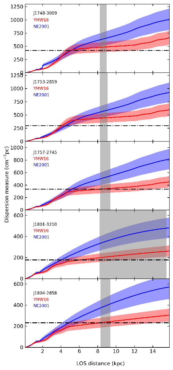
The thermal free electron density model NE20011313 13 https://www.nrl.navy.mil/rsd/RORF/ne2001 (Cordes & Lazio 2002) is widely used to estimate the distances to pulsars based on their measured DM obtained through timing. More recently, Yao et al. 2017 (YMW161414 14 http://119.78.162.254/dmodel/index.php) re-evaluated the electron density model by using more recent independent pulsar distance observations. We compare our dynamically-estimated distances for PSRs J17483009, J17532819, J17572745, J18013210, and J18042825 given in § 5.4 with their DM-derived distances obtained from these electron density models. Note that we do not use PSR J17462758 in this comparison since its distance is not well constrained. We first use the YMW16 and NE2001 models separately to estimate the DM along the LOS of these pulsars (see Fig. 10). Note that we take account of a typical 20 per cent error on these DM values and indicate it with the shaded region in the figure. Based on the measured DM values, we find that the DM-derived distances obtained from the YMW16 model for PSRs J17483009, J17572745, J18013210, and J18042825 are consistent with our dynamics-derived distances within their uncertainties. For PSR J17532819, the DM-derived distance from YMW16 is small compared to its dynamics-derived distance. This indicates that the electron density predicted from YMW16 along the LOS of PSR J17532819 is overestimated, resulting in underestimated distance. As shown in the figure, the DM-derived distances obtained from NE2001 model for all of these pulsars are underestimated compared to their dynamics-estimated distances. By comparing the two models, it is seen that in general the distances estimated by the NE2001 model are underestimated (Kramer et al. 2003, as reported before, see, e.g.,) compared to those estimated by the YMW16 model at a given DM along the LOSs of these pulsars.
We consider all known pulsars that are located within an angular radius of from the GC (i.e. ) and plot their projected distances in the Galactic plane (see Fig. 11). Note that, we use DM-derived distances for these pulsars using the YMW16 model and assume a typical 20% uncertainty. We also plot our dynamically-derived distances for PSRs J17483009, J17532819, J17572745, J18013210, and J18042858 in the same figure. As can be seen, our distance estimates have much smaller uncertainties compared to the DM-derived distances, and these five pulsars are located on the far-side of the Galaxy.

6 Discussion and Conclusion
We report on the timing of recently discovered PSR J17532819, a 18.6 ms pulsar in a 9.3-hr binary orbit. We included this pulsar along with PSRs J17462758, J17483009, J17572745, J18013210, and J18042858 using LT and PKS observations to understand their measurements. The improved timing baselines indicate significant negative measurements for PSRs J17483009, J17532819, J17572745, and J18042858 (see Table 3 and 4). This is the first non-globular cluster pulsar sample that has observed negative measurements in their timing solutions, and they all lie within a few degrees of the GC. In addition, the timing of PSR J18013210 confirmed that it has an extremely low positive measurement, which provides the lowest measured value for a pulsar to date.
Since pulsars are powered by the loss of rotational kinetic energy, they spin-down gradually with a positive intrinsic . Therefore, the negative measurements of PSRs J17483009, J17532819, J17572745, J18042858 and the extremely small measurement of PSR J18013210 are not intrinsic, but induced by dynamics. We modelled the observed values of these pulsars as being due to dynamical acceleration in the Galactic potential along their LOSs. The analysis constrained the model-dependent upper limits on the intrinsic of these pulsars and they are broadly consistent with those of known pulsars (see Fig. 12 and Table 7). Using these model-dependent intrinsic values, we then constrained possible pulsar distances, indicating that PSRs J17483009, J17532819, J17572745, J18013210, and J18042858 are located on the far-side of the Galaxy (see Fig. 11 and Table 7). This is the first time that dynamics have been used to measure the distances to pulsars that are located in the far-side of the Galaxy.
The timing solutions of three pulsars in our sample measured limits on their proper motions (see Table 4). Assuming the Galactic model (Sofue 2013) is correct and , we can determine the maximum possible total proper motion for PSRs J17572745, J18013210, and J18042858 and they are estimated to be 19.2, 12.6, and 13 mas/yr (using Eq. 1). These maximum possible total proper motions are consistent with our timing-measured limits given in Table 4. If the high-significance timing-measured proper motions in the future for these pulsars are greater than the above mentioned values, we can validate the Galactic model and also include any required additional features in the model to explain the observed pulsar motions.
As shown in Fig. 10, our dynamics-derived distances and the DM-derived distances from the YMW16 electron density model for these pulsars are consistent with each other in general within their uncertainties. However, the NE2001 model-derived distances are inconsistent with the dynamics-derived distance. This could be due to difficulties in modelling the electron densities in the inner regions of the Galaxy with high stellar densities and large gas and dust contents towards the centre. Therefore, the independent distance measurements obtained to the pulsars in this study can be used to further improve electron density models.
PSRs J17483009, J17532819, and J18013210 are in binary systems and the timing results indicate that their companions are likely to be white dwarfs. Using the measured limit of PSR J17483009, we derived an independent limit on its intrinsic . Following a similar method, we will be able to measure values of these binary pulsars in the future with more observations and thus, derive their intrinsic values independently with better accuracy (Smits et al. 2011, see). These estimates then can be used to improve their distance measurements.
Most of the Galactic models assume that the mass distribution in the Galaxy is either axially or spherically symmetric for simplicity, in particular within the bulge region. Having more pulsars in the Galactic centre region, we can use their observations to derive dynamics independently to study the Galactic potential, and then update and validate Galactic models including clumpiness in the mass distribution. We can also obtain independent distances to these GC pulsars in the future through parallax measurements using interferometers such as VLBI and then use them in deriving the Galactic potential. The next generation telescopes, such as the Square Kilometre Array, are useful with their outstanding capabilities to discover more pulsars in the GC region and to allow a comprehensive study to constrain the Galactic potential in the central region using pulsar timing in the future.
Acknowledgments
Pulsar research at the Jodrell Bank Centre for Astrophysics and the observations using the Lovell Telescope are supported by a consolidated grant from the STFC in the UK. The Parkes radio telescope is part of the Australia Telescope, which is funded by the Commonwealth of Australia for operation as a National Facility managed by the Commonwealth Scientific and Industrial Research Organisation (CSIRO). D.R.L. acknowledges support from NSF RII Track I award number OIA1458952 and is part of the NANOGrav Physics Frontiers Center which is supported by NSF award 1430284. R.S. acknowledges support from the Australian Research Council grant FL150100148. MB acknowledges ARC Grant CE170100004 (OzGrav).
References
- Abuter et al. (2019) Abuter R., et al., 2019, arXiv e-prints,
- Bassa et al. (2016a) Bassa C. G., et al., 2016a, MNRAS, 456, 2196
- Bassa et al. (2016b) Bassa C. G., et al., 2016b, MNRAS, 460, 2207
- Bates et al. (2011) Bates S. D., et al., 2011, MNRAS, 416, 2455
- Binney & Tremaine (2008) Binney J., Tremaine S., 2008, Galactic Dynamics: Second Edition. Princeton University Press
- Bland-Hawthorn & Gerhard (2016) Bland-Hawthorn J., Gerhard O., 2016, ARA&A, 54, 529
- Bland-Hawthorn et al. (2019) Bland-Hawthorn J., et al., 2019, MNRAS,
- Blandford & Teukolsky (1976) Blandford R., Teukolsky S. A., 1976, ApJ, 205, 580
- Brunthaler et al. (2011) Brunthaler A., et al., 2011, Astronomische Nachrichten, 332, 461
- Cordes & Lazio (2002) Cordes J. M., Lazio T. J. W., 2002, preprint (arXiv:astro-ph/0207156)
- Corongiu et al. (2006) Corongiu A., Possenti A., Lyne A. G., Manchester R. N., Camilo F., D’Amico N., Sarkissian J. M., 2006, ApJ, 653, 1417
- Crawford et al. (2013) Crawford F., et al., 2013, ApJ, 776, 20
- Damour & Taylor (1991) Damour T., Taylor J. H., 1991, ApJ, 366, 501
- Dehnen & Binney (1998) Dehnen W., Binney J., 1998, MNRAS, 294, 429
- Desvignes et al. (2016) Desvignes G., et al., 2016, MNRAS, 458, 3341
- Eatough et al. (2009) Eatough R. P., Keane E. F., Lyne A. G., 2009, MNRAS, 395, 410
- Eatough et al. (2010) Eatough R. P., Molkenthin N., Kramer M., Noutsos A., Keith M. J., Stappers B. W., Lyne A. G., 2010, MNRAS, 407, 2443
- Eatough et al. (2013) Eatough R. P., Kramer M., Lyne A. G., Keith M. J., 2013, MNRAS, 431, 292
- Edwards et al. (2006) Edwards R. T., Hobbs G. B., Manchester R. N., 2006, MNRAS, 372, 1549
- Faulkner et al. (2004) Faulkner A. J., et al., 2004, MNRAS, 355, 147
- Folkner et al. (2009) Folkner W. M., Williams J. G., Boggs D. H., 2009, Interplanetary Network Progress Report, 178, 1
- Folkner et al. (2014) Folkner W. M., Williams J. G., Boggs D. H., Park R. S., Kuchynka P., 2014, Interplanetary Network Progress Report, 196, 1
- Freire et al. (2003) Freire P. C., Camilo F., Kramer M., Lorimer D. R., Lyne A. G., Manchester R. N., D’Amico N., 2003, MNRAS, 340, 1359
- Freire et al. (2017) Freire P. C. C., et al., 2017, MNRAS, 471, 857
- Gardner & Flynn (2010) Gardner E., Flynn C., 2010, MNRAS, 405, 545
- Genzel et al. (2000) Genzel R., Pichon C., Eckart A., Gerhard O. E., Ott T., 2000, MNRAS, 317, 348
- Ghez et al. (2005) Ghez A. M., Salim S., Hornstein S. D., Tanner A., Lu J. R., Morris M., Becklin E. E., Duchêne G., 2005, ApJ, 620, 744
- Ghez et al. (2008) Ghez A. M., et al., 2008, ApJ, 689, 1044
- Gillessen et al. (2009) Gillessen S., Eisenhauer F., Trippe S., Alexander T., Genzel R., Martins F., Ott T., 2009, ApJ, 692, 1075
- Gonzalez et al. (2011) Gonzalez M. E., et al., 2011, ApJ, 743, 102
- Guinot (1988) Guinot B., 1988, A&A, 192, 370
- Haslam et al. (1982) Haslam C. G. T., Stoffel H., Salter C. J., Wilson W. E., 1982, A&AS, 47, 1
- Hobbs & Edwards (2012) Hobbs G., Edwards R., 2012, Tempo2: Pulsar Timing Package, Astrophysics Source Code Library (ascl:1210.015)
- Hobbs et al. (2004a) Hobbs G., et al., 2004a, MNRAS, 352, 1439
- Hobbs et al. (2004b) Hobbs G., Lyne A. G., Kramer M., Martin C. E., Jordan C., 2004b, MNRAS, 353, 1311
- Hobbs et al. (2005) Hobbs G., Lorimer D. R., Lyne A. G., Kramer M., 2005, MNRAS, 360, 974
- Hobbs et al. (2006) Hobbs G. B., Edwards R. T., Manchester R. N., 2006, MNRAS, 369, 655
- Hobbs et al. (2012) Hobbs G., et al., 2012, MNRAS, 427, 2780
- Honma et al. (2012) Honma M., et al., 2012, PASJ, 64, 136
- Hotan et al. (2004) Hotan A. W., van Straten W., Manchester R. N., 2004, PASA, 21, 302
- Jacoby et al. (2006) Jacoby B. A., Cameron P. B., Jenet F. A., Anderson S. B., Murty R. N., Kulkarni S. R., 2006, ApJ, 644, L113
- Kaspi et al. (1994) Kaspi V. M., Taylor J. H., Ryba M., 1994, ApJ, 428, 713
- Keith et al. (2009) Keith M. J., Eatough R. P., Lyne A. G., Kramer M., Possenti A., Camilo F., Manchester R. N., 2009, MNRAS, 395, 837
- Knispel et al. (2013) Knispel B., et al., 2013, ApJ, 774, 93
- Kramer et al. (2003) Kramer M., et al., 2003, MNRAS, 342, 1299
- Kramer et al. (2006) Kramer M., et al., 2006, Science, 314, 97
- Lazaridis et al. (2009) Lazaridis K., et al., 2009, MNRAS, 400, 805
- Lorimer (2011) Lorimer D. R., 2011, SIGPROC: Pulsar Signal Processing Programs, Astrophysics Source Code Library (ascl:1107.016)
- Lorimer & Kramer (2005) Lorimer D. R., Kramer M., 2005, Handbook of Pulsar Astronomy. Cambridge University Press
- Lorimer et al. (2006) Lorimer D. R., et al., 2006, MNRAS, 372, 777
- Lorimer et al. (2015) Lorimer D. R., et al., 2015, MNRAS, 450, 2185
- Lynch et al. (2012) Lynch R. S., Freire P. C. C., Ransom S. M., Jacoby B. A., 2012, ApJ, 745, 109
- Lyne et al. (1998) Lyne A. G., et al., 1998, MNRAS, 295, 743
- Manchester et al. (2001) Manchester R. N., et al., 2001, MNRAS, 328, 17
- Manchester et al. (2005) Manchester R. N., Hobbs G. B., Teoh A., Hobbs M., 2005, AJ, 129, i
- Matthews et al. (2016) Matthews A. M., et al., 2016, ApJ, 818, 92
- McMillan (2011) McMillan P. J., 2011, MNRAS, 414, 2446
- McMillan (2016) McMillan P. J., 2016, GalPot: Galaxy potential code, Astrophysics Source Code Library (ascl:1611.006)
- McMillan (2017) McMillan P. J., 2017, MNRAS, 465, 76
- McWilliam & Zoccali (2010) McWilliam A., Zoccali M., 2010, ApJ, 724, 1491
- Mickaliger (2013) Mickaliger M. B., 2013, PhD thesis, West Virginia University
- Mickaliger et al. (2012) Mickaliger M. B., et al., 2012, ApJ, 759, 127
- Mickaliger et al. (2018) Mickaliger M. B., McEwen A. E., McLaughlin M. A., Lorimer D. R., 2018, MNRAS, 479, 5413
- Morello et al. (2019) Morello V., et al., 2019, MNRAS, 483, 3673
- Morris et al. (2002) Morris D. J., et al., 2002, MNRAS, 335, 275
- Nataf et al. (2010) Nataf D. M., Udalski A., Gould A., Fouqué P., Stanek K. Z., 2010, ApJ, 721, L28
- Navarro et al. (1996) Navarro J. F., Frenk C. S., White S. D. M., 1996, ApJ, 462, 563
- Ness et al. (2012) Ness M., et al., 2012, ApJ, 756, 22
- Ng et al. (2014) Ng C., et al., 2014, MNRAS, 439, 1865
- Ng et al. (2015) Ng C., et al., 2015, MNRAS, 450, 2922
- Nice & Taylor (1995) Nice D. J., Taylor J. H., 1995, ApJ, 441, 429
- Perera et al. (2017) Perera B. B. P., et al., 2017, MNRAS, 468, 2114
- Petit (2003) Petit G., 2003, in 35th Annual Precise Time and Time Interval (PTTI) Meeting, San Diego, December 2003. pp 307–317
- Petit & Tavella (1996) Petit G., Tavella P., 1996, A&A, 308, 290
- Piffl et al. (2014) Piffl T., et al., 2014, MNRAS, 445, 3133
- Portail et al. (2017) Portail M., Gerhard O., Wegg C., Ness M., 2017, MNRAS, 465, 1621
- Prager et al. (2017) Prager B. J., Ransom S. M., Freire P. C. C., Hessels J. W. T., Stairs I. H., Arras P., Cadelano M., 2017, ApJ, 845, 148
- Ransom (2011) Ransom S., 2011, PRESTO: PulsaR Exploration and Search TOolkit, Astrophysics Source Code Library (ascl:1107.017)
- Reid et al. (2009) Reid M. J., Menten K. M., Zheng X. W., Brunthaler A., Xu Y., 2009, ApJ, 705, 1548
- Reid et al. (2014) Reid M. J., et al., 2014, ApJ, 783, 130
- Schönrich (2012) Schönrich R., 2012, MNRAS, 427, 274
- Schönrich et al. (2010) Schönrich R., Binney J., Dehnen W., 2010, MNRAS, 403, 1829
- Shklovskii (1970) Shklovskii I. S., 1970, SvA, 13, 562
- Smits et al. (2011) Smits R., Tingay S. J., Wex N., Kramer M., Stappers B., 2011, A&A, 528, A108
- Sofue (2013) Sofue Y., 2013, PASJ, 65, 118
- Sofue (2017) Sofue Y., 2017, PASJ, 69, R1
- Stairs et al. (2002) Stairs I. H., Thorsett S. E., Taylor J. H., Wolszczan A., 2002, ApJ, 581, 501
- Taylor (1992) Taylor J. H., 1992, RSPTA, 341, 117
- Taylor & Weisberg (1989) Taylor J. H., Weisberg J. M., 1989, ApJ, 345, 434
- Vasiliev (2019) Vasiliev E., 2019, MNRAS, 484, 2832
- Verbunt et al. (2017) Verbunt F., Igoshev A., Cator E., 2017, A&A, 608, A57
- Wolszczan et al. (1989) Wolszczan A., Kulkarni S. R., Middleditch J., Backer D. C., Fruchter A. S., Dewey R. J., 1989, New Astron., 337, 531
- Yao et al. (2017) Yao J. M., Manchester R. N., Wang N., 2017, ApJ, 835, 29
- van Straten et al. (2011) van Straten W., Demorest P., Khoo J., Keith M., Hotan A., et al. 2011, PSRCHIVE: Development Library for the Analysis of Pulsar Astronomical Data, Astrophysics Source Code Library (ascl:1105.014)
- van Straten et al. (2012) van Straten W., Demorest P., Oslowski S., 2012, Astronomical Research and Technology, 9, 237
Appendix A Transverse velocity of the pulsar and the Shklovskii contribution
We denote the peculiar velocity of the Sun as , where the unit vectors of the components are in the direction from the Sun towards the GC, in the direction of the Galactic rotation, and in the direction perpendicular to the Galactic plane, respectively. Then the total velocity of the Sun
| (8) |
where is the velocity of the local standard of rest for the Sun, or the circular Galactic rotational velocity at the radius of Sun . For our calculation, we assume km/s (Schönrich et al. 2010) and obtain the Galactic rotation from Galactic mass distribution models given in § 5.2. The main Galactic model we use in this study (Sofue 2017) results in km/s, which is the value they adopted in their model from Honma et al. 2012. Then the peculiar velocity, or the 3-dimensional space velocity, of the pulsar is defined as in the same coordinate system as before. The total velocity of the pulsar including its local standard of rest,
| (9) |
where is the Galactic rotational velocity of the pulsar at its projected radial distance on to the Galactic plane and is the angle subtended at the GC between the position of the Sun and the projected position of the pulsar on the Galactic plane (see Fig. B.1 in Verbunt et al. 2017, for a schematic diagram). The angle can be expressed as
| (10) |
Using the above coordinate system, the relative velocity of the pulsar with respect to the Sun
| (11) |
To express the relative velocity in the Galactic coordinate system , we write the unit vectors in above coordinate system as
| (12) |
We then write the relative velocity of the pulsar for its given with respect to the Sun in Galactic coordinates as
| (13) |
and
| (14) |
respectively. We finally calculate the transverse velocity of the pulsar to be . The derivation of the above expressions are given in Verbunt et al. 2017 in detail.
In § 5, for a given 3-dimensional pulsar space velocity of , we randomly calculate (where ), leading to a transverse velocity of using Eq. 13 and 14. We perform 1000 trials for a given and then obtain the average , and then calculate the Shklovskii effect . We note that is a function of and thus, it varies along the LOS of the pulsar for a given , and then . For instance, this variation in can be seen in Fig. 5.