Deep Iterative Reconstruction for Phase Retrieval
Abstract
Classical phase retrieval problem is the recovery of a constrained image from the magnitude of its Fourier transform. Although there are several well-known phase retrieval algorithms including the hybrid input-output (HIO) method, the reconstruction performance is generally sensitive to initialization and measurement noise. Recently, deep neural networks (DNNs) have been shown to provide state-of-the-art performance in solving several inverse problems such as denoising, deconvolution, and superresolution. In this work, we develop a phase retrieval algorithm that utilizes two DNNs together with the model-based HIO method. First, a DNN is trained to remove the HIO artifacts, and is used iteratively with the HIO method to improve the reconstructions. After this iterative phase, a second DNN is trained to remove the remaining artifacts. Numerical results demonstrate the effectiveness of our approach, which has little additional computational cost compared to the HIO method. Our approach not only achieves state-of-the-art reconstruction performance but also is more robust to different initialization and noise levels.
Keywords phase retrieval deep learning inverse problems image reconstruction
1 Introduction
The classical phase retrieval problem is the recovery of a constrained signal from the magnitude of its Fourier transform, or equivalently from its autocorrelation. This problem is encountered in a variety of applications in science and engineering such as crystallography [1], microscopy [2, 3], astronomy [4], optical imaging [5, 6], and speech processing [7]. Although a unique solution almost always exists for most of the practical scenarios [8], solving the phase retrieval problem is generally a difficult task because of the inherent ill-posedness and nonlinearity involved.
Although there are several approaches developed for phase retrieval, each suffers from different limitations. Alternating projection-based methods, including the hybrid input-output (HIO) algorithm, are the most commonly used methods because of their low computational complexity and image generality [9, 10]. This class of methods alternates between the space and frequency domains by imposing the available information in each domain through projections [9, 11, 12, 10]. However, some of these projections involve non-convex sets, and hence convergence to the global solution can not be guaranteed. The resulting reconstructions may have artifacts and errors mostly due to being stuck in local minima or amplification of noise in the solution. More recent phase retrieval algorithms have been developed to overcome some of these limitations. Examples include semi-definite programming-based approaches [13, 14, 15], regularization-based methods [16, 17, 18], global optimization methods [19], and Wirtinger flow and its variants [20].
Deep neural networks (DNNs) [21] have been shown to be successful in various inverse problems in imaging in the last few years [22]. There are mainly two different approaches in exploiting DNNs for the solution of inverse problems. In the first class of approaches, a DNN is used to reconstruct the unknown image directly from an available measurement or from an initial estimate obtained with a simple model-based inversion approach. Hence, these approaches exploit DNNs either to perform direct inversion or to improve a rough estimate that may involve artifacts or errors. For this, a DNN is trained by minimizing a loss function between the ground truth images and the available measurements or estimates. This approach has been utilized to solve several inverse problems [23, 24, 25, 26], including phase retrieval as encountered in holography, lensless imaging and Fourier ptychography [27, 3, 28]. Moreover, in the second class of approaches, DNNs are utilized for the regularization of model-based inversion methods by using plug-and-play regularization and its variants [29, 30]. This approach has been also applied to several inverse problems [31, 32, 33, 34] including phase retrieval [17].
In this paper, we develop a hybrid phase retrieval algorithm that utilizes DNNs with a model-based inversion approach. Here, the used model-based inversion approach is the well-known HIO method, which incorporates the physical model and the constraints into the solution, but may lead to artifacts. The main idea in the developed method is to use a DNN in an iterative manner with the HIO method to remove the artifacts. The developed approach consists of two main stages: the iterative DNN-HIO stage and the final DNN stage. For the iterative DNN-HIO stage, a DNN is trained to remove the HIO artifacts. This trained DNN is then used iteratively with the HIO method to generate an intermediate reconstruction. In the final stage, the intermediate reconstructions are used to train a second DNN to remove the remaining artifacts. The performance of the developed approach is compared with the classical and state-of-the-art methods through numerical simulations. The results demonstrate the effectiveness of our approach, which has relatively little additional computational cost compared to HIO. Our approach not only achieves state-of-the-art reconstruction performance, but also is more robust to different initialization and noise levels.
The rest of this paper is organized as follows. The classical phase retrieval problem is described in Section 2. Related work on phase retrieval and DNN-based methods are discussed in Section 3. Section 4 presents the developed approach. The performance of the approach is compared with the classical and state-of-the-art methods in Section 5 through simulations. Finally, we summarize the results and conclude in Section 6.
2 Phase Retrieval Problem
In the classical phase retrieval problem, available measurements can be modeled as
| (1) |
where denotes the noisy Fourier intensity measurements, is the -point DFT matrix, and represents the unknown image of interest. The unknown image is assumed to be non-negative, real-valued and have finite support. Moreover, denotes the measurement noise, and is a scaling parameter that controls the signal-to-noise ratio (SNR). The noise is generally assumed to be Poisson-distributed, and here its normal approximation [17] is used.
For two or higher dimensional real-valued discrete signals with finite support, Fourier intensity measurements at discrete frequencies, , can uniquely determine the unknown signal, . To guarantee uniqueness, for an image with support x, the magnitude of its -point oversampled DFT with should be provided [8]. In this work, is chosen as for simplicity.
3 Related Work
3.1 Alternating Projection Methods for Phase Retrieval
Alternating projection-based methods are widely used for phase retrieval. In the classical Gerchberg-Saxton (GS) algorithm [11], magnitude constraints are iteratively imposed in space and Fourier domains to reconstruct the unknown signal. The error reduction (ER) algorithm is a modified version of the GS algorithm, which uses other space domain constraints than the magnitude in the space domain [12]. The most commonly used alternating projection-based method is the HIO algorithm [10], which is developed based on the ER algorithm.
Similar to the ER algorithm, in the HIO method, Fourier magnitude constraint and space domain constraints (such as support, non-negativity, and real valuedness) are iteratively used. However, unlike ER, HIO does not force the iterates to satisfy the constraints exactly, but it uses the iterates to eventually drive the algorithm to a solution that satisfy the constraints [10]. The HIO iterations can be expressed as follows:
| (2) |
where
| (3) |
Here, is the reconstruction at the iteration, denotes the inverse DFT matrix, represents the element-wise (Hadamard) multiplication operation, is a constant parameter (with a typical value of ) and is the set of indices for which violates the space domain constraints [10]. Although the convergence behavior of the HIO method cannot be completely analyzed, it often converges to a reasonably good solution empirically in a wide variety of applications. However, the HIO reconstructions may have artifacts and errors mostly due to being trapped in local minima or amplification of noise in the solution. Variants of the HIO method have also been proposed to improve its performance [9].
3.2 DNN-based Methods for Inverse Problems
In the last decade, DNNs have been successfully used for the solution of various inverse problems including denoising, deconvolution, and superresolution [22]. There are two main approaches in utilizing DNNs for solving inverse problems.
In the first class of approaches, a DNN is used to reconstruct the unknown image directly from an available measurement or from an initial estimate obtained with a simple model-based inversion. That is, these approaches exploit DNNs either to solve end-to-end inverse problems or to improve a rough estimate that may have artifacts or errors. For this purpose, a DNN is trained by minimizing a loss function using a dataset containing the ground truth images and the measurements (or the initial estimates). In general, this approach provides a faster reconstruction than a model-based inversion approach since it works in a non-iterative feed-forward fashion to solve the problem. However, a DNN usually needs specialized training and dataset for each inverse problem, which reduces its flexibility to handle different inverse problems. More importantly, this approach works successfully only when the measurements or the initial estimates used for reconstruction are similar in appearance to the ground truth images. This approach has been used to solve several inverse problems in imaging applications such as denoising [23], deconvolution [24, 35], superresolution [25, 36], tomography [26], holographic image reconstruction [3], phase retrieval for phase objects [27], and Fourier ptychography [28].
In the second class of approaches, DNNs are utilized for the regularization of model-based inversion methods. The classical approach to regularization is to formulate the inverse problem as a maximum posterior (MAP) estimation problem by incorporating the prior statistical knowledge about the unknown image. This yields to an optimization problem involving a likelihood term, which quantifies the fidelity with the model, and a prior term, which is also known as the regularization term [37]. By variable splitting techniques, this optimization problem can be divided into sub-problems to deal with the likelihood and prior terms separately. In particular, the sub-problem containing the prior term corresponds to a denoising problem, which can be solved with any denoising algorithm. This is the main idea in plug-and-play regularization [29, 30]. Recently, DNN-based denoisers are used for plug-and-play regularization because DNNs provides state-of-the-art performance in denoising. Plug-and-play regularization using DNN-based denoisers is a flexible model-based approach since the same denoiser can be used for the solution of different inverse problems. This approach has been applied to several inverse problems including deconvolution, denoising, superresolution and demosaicking [31, 32, 33, 34], as well as phase retrieval [17, 38].

4 DNN-based Iterative Approach
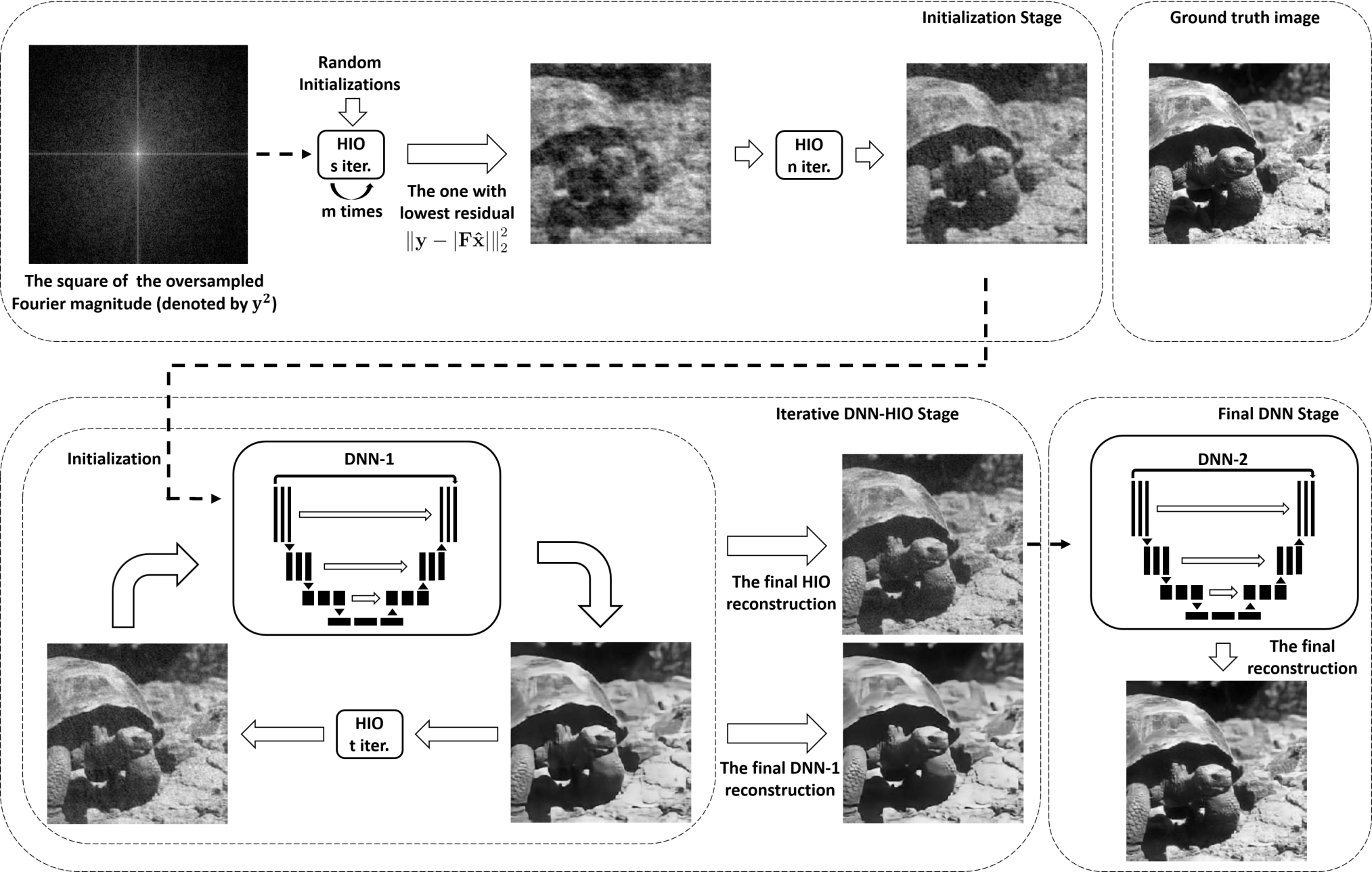
Our deep learning-based hybrid approach utilizes DNNs together with the HIO method. The main idea in our approach is to use the HIO method to directly incorporate the physical model and the constraints into the reconstruction, and DNNs to improve the resulting HIO reconstructions. The first DNN, namely DNN-1, is trained to remove the artifacts of the initial HIO reconstructions, and is used iteratively with the HIO method to generate an intermediate reconstruction. Then, a second DNN, namely DNN-2, is trained to remove the remaining artifacts after this iterative stage. The output of DNN-2 is the final reconstruction of our method. The overall approach is illustrated in Fig. 1 using representative images for the input and output of each step. A preliminary version of this iterative approach was presented in [39].
As shown in Fig. 1, the approach consists of three stages: the initialization stage, the iterative DNN-HIO stage and the final DNN stage. The initialization stage aims to achieve robustness to initialization. For this aim, the HIO reconstructions with different random initialization are obtained and the one that provides Fourier magnitude closest to the given measurement is chosen as the input (initialization) for the iterative stage. In the iterative DNN-HIO stage, a DNN and the HIO method are used iteratively to generate an intermediate reconstruction. This DNN is trained using the HIO reconstruction at the output of the initialization stage with the ground truth images. Hence this training aims to remove the HIO artifacts at the output of the initialization stage, but this can be performed to some extent. After this iterative stage, the intermediate reconstructions have less artifacts than the initial HIO reconstructions. In the final DNN stage, the intermediate reconstructions are used with the ground truth images to train a second DNN to remove the remaining artifacts.
As DNN architectures, the modified U-net architecture developed in [26] is used. This architecture, which is shown in Fig. 2, works in a non-iterative feed-forward fashion to solve general inverse problems in imaging. In particular, in [26], this is used to obtain reconstructions for computed tomography. Here we use the same architecture in an iterative manner with the HIO method to solve the phase retrieval problem.
This architecture is the modified version of the original U-net architecture [40]. The original U-net is developed for biomedical image segmentation and it exploits encoding and decoding convolutional layers with skip connections between symmetric downsampling and upsampling convolutional layers [22]. These features were shown to be useful for solving many inverse problems including denoising [41], image inpainting [42], optical flow estimation [43] and computed tomography [26]. In addition to these features, the modified U-net architecture contains batch normalization layers and direct skip connection between the input and output. These modifications help the DNN to better learn the residual between the input and output images [23].
In what follows, we provide the details of each stage in our approach.
4.1 Initialization Stage
Due to the nonlinearity (and non-convexity) involved in the phase retrieval problem, the reconstruction algorithms are generally sensitive to initialization. Here, to increase the robustness of our approach, a particular initialization procedure described earlier in [17] is used. In this procedure, first, the HIO method is run with different random initialization for a small number of iterations. Then, the reconstruction with the lowest residual is used for another HIO run for a larger number of iterations. The final reconstruction is used as the input (initialization) for the iterative DNN-HIO stage.
4.2 Iterative DNN-HIO Stage
As mentioned before, although the HIO method benefits from the physical model and the constraints during the reconstruction process, the results may have artifacts and errors caused mostly by the presence of noise or being stuck in local minima. In this stage, a DNN (namely DNN-1) and the HIO method are used alternately to solve the phase retrieval problem.
DNN-1 is trained to remove the artifacts of the HIO method after the initialization stage. That is, DNN-1 is trained by using a dataset containing the true images and their corresponding HIO reconstructions at the output of the initialization stage. Then, the HIO method and the trained DNN are used in an iterative manner until the reconstructions start to change slightly. This iterative approach aims to improve the reconstructions by escaping from local minima and reducing artifacts.
More specifically, at the iteration of this stage, the last HIO reconstruction, , is used as the input for DNN-1. Then, the improved reconstruction, , at the output of DNN-1 is used as the initialization for the HIO method, which is run for a small number of iterations. This iterative procedure continues until the normalized error between two consecutive DNN-1 reconstructions, i.e. , is smaller than .
As the iterations proceed, both the reconstructions of DNN-1 and HIO are improved. In particular, the HIO method better preserves the high spatial frequencies of the original image, which represent sudden spatial changes in the image, compared to DNN-1, while DNN-1 provides reconstructions with less artifacts. This has two main reasons. First, DNNs generally smooth out the high frequencies during its learning process when they are trained with a mean squared error (MSE) based loss, which is a common problem in DNNs [22]. Moreover, the main task of DNN-1 here is to remove the large artifacts, which inherently comes with the side effect of smoothing (i.e. low-pass filtering). Secondly, unlike DNN-1, the HIO method uses the available measurements together with the forward model, which helps to preserve high frequencies, although it comes with artifacts. The final HIO reconstruction is used as the input for the last stage in order to preserve high frequencies in the final reconstruction.
4.3 Final DNN Stage
In this last stage, a second DNN (namely DNN-2) is used to improve the reconstruction of the iterative DNN-HIO stage by removing the remaining artifacts. The reason for using a different DNN here is that DNN-1 is trained to remove the HIO artifacts at the output of the initialization stage, but the reconstructions of the iterative DNN-HIO stage have less artifacts than before (for example, see Fig. 1). Hence training another DNN enables to obtain improved reconstructions with better preserved high frequencies (details) and reduced artifacts.
DNN-2 is trained to remove the artifacts of the iterative DNN-HIO stage. That is, DNN-2 is trained by using a dataset containing the same ground truth images and the corresponding HIO reconstructions at the output of the iterative DNN-HIO stage. As mentioned before, MSE-based loss function is used for training, but different loss functions could also be utilized to better preserve high frequencies. This trained DNN is used in a non-iterative feed-forward fashion to obtain the final reconstruction of our method.
5 Numerical Results
Here we present numerical simulations to illustrate the effectiveness of our approach. For this, we consider a large image dataset and compare the reconstruction performance of the developed approach with the classical and state-of-the-art phase retrieval methods.
To compare the algorithms in terms of noise tolerance, image generality, and computational efficiency, the reconstruction performance is investigated using two different kind of images, which are called natural and unnatural images. For training DNN-1 and DNN-2, only natural images are used. This training dataset consists of natural images. These include training and validation images of Berkeley segmentation dataset (BSD) [44], selected images from validation set of ImageNet database [45, 31], and randomly chosen images of Waterloo Exploration Database [46].
For testing, both natural and unnatural images are used. This test dataset consists of images containing natural and unnatural images. These include test images of BSD, Kodak dataset images [47], natural and unnatural images taken from [17]. The unnatural image dataset consists of images acquired by scanning electron microscopes and telescopes, as shown in Fig. 3. The pixel values of all images are between and , and all are of size .


The noisy Fourier measurements were simulated using Eqn. 1 with , resulting in an average SNR of dB (where SNR ). These measurements were used to obtain the initial HIO reconstructions at the output of the initialization stage. DNN-1 was trained using these reconstructions and the true images. Likewise, DNN-2 was trained using the true images and the HIO reconstructions of the iterative DNN-HIO stage. Although only natural images were used in training, the developed approach with the trained DNNs was tested using both natural and unnatural images.
Training was performed by minimizing the MSE-based loss between the true images and the output of each DNN. Stochastic gradient descent algorithm with momentum was used for the optimization [48]. All computations were done using MATLAB with MatConvNet toolbox [49] and NVIDIA Geforce GTX TITAN X GPU. The total training times for DNN-1 and DNN-2 were about hours (for iterations) and hours (for iterations), respectively.
In the initialization stage, the HIO method was first run with different random initialization for iterations. Then, the reconstruction with the lowest residual was used for another HIO run for iterations. The resulting reconstruction was input to the iterative DNN-HIO stage as shown in Fig. 1. In this stage, each time the HIO method was run for iterations.
After the testing phase, the reconstructions of the developed approach were compared with the true images using peak signal-to-noise ratio (PSNR) and structural similarity index (SSIM) [50]. For comparison, the reconstructions of the HIO method and prDeep [17], one of the state-of-the-art deep learning-based phase retrieval algorithms, were also obtained. Both the developed algorithm and prDeep were initialized with the output of the initialization stage. The HIO reconstruction used for comparison was the output of this initialization stage.
In Table 1, the average reconstruction performance of the algorithms for test images and Monte Carlo runs are given for different amount of Poisson noise (). As seen in the table, for all cases, the developed method outperforms the HIO and prDeep methods in terms of both PSNR and SSIM, while requiring little additional runtime compared to HIO. As another benchmark, the results at the output of DNN-1 and iterative DNN-HIO stages are also provided in the table to show performance gains obtained by the iterative approach. The results illustrates that, by utilizing a DNN in an iterative manner with the HIO method, many of the HIO artifacts can be successfully removed while preserving the image characteristics. This iterative approach with the additional DNN (DNN-2) is the overall method, which provides the best reconstruction performance.
| (Avg. SNR: 33.39 dB) | Avg. PSNR (dB) | Avg. SSIM | Avg. runtime (sec.) | ||||
|---|---|---|---|---|---|---|---|
| Overall | Natural | Unnatural | Overall | Natural | Unnatural | ||
| The HIO method (The output of the initialization stage) | 18.97 | 18.92 | 20.78 | 0.28 | 0.29 | 0.26 | 55.40 |
| DNN-1 | 20.76 | 20.77 | 20.33 | 0.33 | 0.33 | 0.20 | 55.47 |
| Iterative DNN-HIO (The final HIO reconstruction) | 21.63 | 21.60 | 22.75 | 0.47 | 0.47 | 0.26 | 59.07 |
| PrDeep | 23.45 | 23.49 | 21.72 | 0.51 | 0.51 | 0.24 | 169.81 |
| Developed method | 23.61 | 23.60 | 24.02 | 0.53 | 0.53 | 0.31 | 59.14 |
| (Avg. SNR: 31.66 dB) | Avg. PSNR (dB) | Avg. SSIM | Avg. runtime (sec.) | ||||
| Overall | Natural | Unnatural | Overall | Natural | Unnatural | ||
| The HIO method (The output of the initialization stage) | 18.07 | 18.02 | 19.97 | 0.21 | 0.21 | 0.14 | 55.61 |
| DNN-1 | 19.69 | 19.68 | 20.06 | 0.26 | 0.26 | 0.18 | 55.69 |
| Iterative DNN-HIO (The final HIO reconstruction) | 21.07 | 21.03 | 22.82 | 0.41 | 0.42 | 0.25 | 60.29 |
| PrDeep | 22.06 | 22.09 | 20.91 | 0.44 | 0.44 | 0.22 | 171.02 |
| Developed method | 22.87 | 22.85 | 23.50 | 0.47 | 0.48 | 0.29 | 60.35 |
| (Avg. SNR: 30.40 dB) | Avg. PSNR (dB) | Avg. SSIM | Avg. runtime (sec.) | ||||
| Overall | Natural | Unnatural | Overall | Natural | Unnatural | ||
| The HIO method (The output of the initialization stage) | 17.34 | 17.30 | 18.72 | 0.16 | 0.17 | 0.10 | 55.78 |
| DNN-1 | 18.75 | 18.76 | 18.65 | 0.21 | 0.21 | 0.14 | 55.86 |
| Iterative DNN-HIO (The final HIO reconstruction) | 20.08 | 20.03 | 22.22 | 0.35 | 0.36 | 0.20 | 60.99 |
| PrDeep | 20.69 | 20.70 | 20.38 | 0.37 | 0.38 | 0.18 | 172.47 |
| Developed method | 21.80 | 21.77 | 22.79 | 0.41 | 0.41 | 0.25 | 61.05 |


Sample reconstructions for a natural image in the test dataset are shown in Fig. 4. As seen from the figures, the developed approach provides the best reconstruction visually as well as in terms of used quantitative image quality measures (PSNR and SSIM). In fact, our approach generally does not introduce artifacts and errors like the HIO and prDeep methods. As mentioned before, removing artifacts sometimes causes the side effect of smoothing, as illustrated with the zoomed results given in Fig. 4.
For the same test image, Fig. 5 shows the several intermediate reconstructions obtained with the developed approach. The reconstructions at the output of each stage, including the initialization stage, iterative DNN-HIO stage, and the final DNN stage, are shown here, together with their respective PSNR and SSIM values. These clearly illustrate the contribution of each stage. For example, the improvement obtained with the final DNN-2 stage can be understood by comparing the final reconstruction in Fig. 5f with the reconstructions at the output of the iterative stage as given in Figures 5d and 5e. In fact, this final reconstruction is much better than all the other reconstructions both visually and quantitatively. Moreover, to demonstrate the usefulness of the iterative use of HIO with DNN-1, the reconstructions obtained after the first iteration are also provided in Figures 5b and 5c. Comparing these with Figures 5d and 5e illustrates that, although even a single iteration helps to improve the initial HIO reconstruction, iterations until convergence can provide much significant improvement. Note that after DNN-1 (see Fig. 5b), the reconstruction suffers from over-smoothing, and when this is input to HIO (see Fig. 5c) some high frequency information is recovered but with artifacts. As the iterations proceed, both over-smoothing and artifacts are reduced.


To assess the performance of different algorithms in terms of image generality, the results for both natural and unnatural test images are separately provided in Table 1. As seen in the table, although the DNNs were trained by using only natural images, the developed method shows the best reconstruction performance not only for natural images but also for unnatural images, which have distinct statistics from natural images. In particular, the performance of the prDeep method substantially degrades for unnatural images, as expected, since its reconstruction relies on a regularization prior learned from natural images. To illustrate these points, sample reconstructions for an unnatural image in the test dataset are shown in Fig. 6.
The developed approach also appears to be robust to different noise levels. As seen from the table, the reconstruction performance of the approach surpasses the other methods for different noise levels () as well, even though the DNNs were trained only for a specific noise level ().
As mentioned before, phase retrieval algorithms are generally sensitive to initialization because of the nonlinearity involved in the problem. To illustrate the robustness of the developed approach to different initialization and image characteristics, the PSNR and SSIM histograms are provided in Fig. 7 for each method (when ). These include reconstructions obtained with distinct test images and Monte Carlo runs, which means that different initialization is used for each test image. As seen from the histograms, although the histogram for the prDeep reconstructions has more counts in higher PSNR and SSIM values, our method attains a higher average PSNR and SSIM, as well as a smaller spread around these averages. These results suggest that the performance of the developed approach is more robust to different initialization and image statistics compared to HIO and prDeep.
Sample reconstructions illustrating the performance of the developed approach for different initialization are shown in Fig. 8. Here different HIO reconstructions of the same image are used as an initialization for prDeep and the developed method. As seen, for the HIO initialization with the lower PSNR and SSIM values, prDeep reconstruction has more artifacts than the developed method. Hence, Fig. 7 and 8 together demonstrate that the developed method is more robust to initialization than prDeep.
The average runtime of each method is also given in Table 1. As seen, the HIO and the developed method are roughly three-fold faster than prDeep. In fact, the runtime of the HIO initialization stage approximately corresponds to of the runtime of the developed method. Hence our approach not only outperforms the prDeep and HIO methods in terms of reconstruction quality, but also is computationally more efficient than prDeep and achieves a computational efficiency almost comparable with the HIO method.
6 Conclusions
In this paper, we developed a phase retrieval approach that utilizes two DNNs with the model-based HIO method. The key idea in the approach is the iterative use of a DNN with the HIO method, which simultaneously incorporates the physical model and the constraints into the solution, while avoiding the reconstruction artifacts. The performance of the developed approach is also compared with the classical and state-of-the-art methods through various numerical simulations. The results demonstrate the effectiveness of our approach both in terms of reconstruction quality and computational efficiency. Our approach not only achieves state-of-the-art reconstruction performance but also is more robust to initialization, different noise levels, and image statistics. Moreover, the developed approach achieves a computational efficiency almost comparable with the HIO method.
Note that the developed method contains two DNNs, DNN-1 and DNN-2, each of which is trained to remove HIO artifacts. That is, DNN-1 is trained to remove the artifacts of HIO reconstructions at the output of the initialization stage and DNN-2 is trained to remove the artifacts of HIO reconstructions at the output of iterative DNN-HIO stage. These reconstructions have different amount of artifacts, as one can observe from the PSNR and SSIM values in Table 1. One would expect the trained weights of these two DNNs to vastly differ since each DNN is trained to remove different amount of HIO artifacts. To explore this, we analyzed the frequency response of the first convolution filters in each trained DNN. Almost half of these filters in DNN-1 have similar characteristics, which effectively correspond to low pass filters. On the other hand, DNN-2 filters have varying frequency responses and a very small fraction of these filters are low-pass. This indicates that the detailed differences between the input and the desired output images (like edges) are lost more in the first convolution filters of DNN-1 and do not propagate much through the network. This is expected since DNN-1 is trained using inputs with larger amount of HIO artifacts. The low-pass behavior of many of the input filters of DNN-1 can be the reason why DNN-1 is less successful in learning the details and leads to over-smoothed images at its output. A more detailed analysis of the filters in DNNs would provide a better understanding of the developed approach, which will be a topic for future study. The joint training of DNNs can be another promising research direction in this respect.
To conclude, the developed hybrid method offers state-of-the-art reconstruction performance as well as computational efficiency for the phase retrieval problem. We believe that the hybrid use of DNNs with model-based approaches, such as in an iterative manner as illustrated in this paper, may play a key role in developing more reliable algorithms for phase retrieval and nonlinear inverse problems in general.
References
- [1] R. P. Millane. Phase retrieval in crystallography and optics. J. Opt. Soc. Am. A, 7(3):394–411, Mar 1990.
- [2] Guoan Zheng, Roarke Horstmeyer, and Changhuei Yang. Wide-field, high-resolution fourier ptychographic microscopy. Nature Photonics, 7(9):739, 2013.
- [3] Yair Rivenson, Yibo Zhang, Harun Günaydın, Da Teng, and Aydogan Ozcan. Phase recovery and holographic image reconstruction using deep learning in neural networks. Light: Science & Applications, 7(2):17141, 2018.
- [4] J C. Dainty and James Fienup. Phase retrieval and image reconstruction for astronomy. Image Recovery: Theory Appl, 13:231–275, 01 1987.
- [5] Adriaan Walther. The question of phase retrieval in optics. Optica Acta: International Journal of Optics, 10(1):41–49, 1963.
- [6] Timothy J. Schulz and Donald L. Snyder. Image recovery from correlations. J. Opt. Soc. Am. A, 9(8):1266–1272, Aug 1992.
- [7] Lawrence Rabiner and Biing-Hwang Juang. Fundamentals of speech recognition. Prentice-Hall, Inc., 1993.
- [8] M. Hayes. The reconstruction of a multidimensional sequence from the phase or magnitude of its fourier transform. IEEE Transactions on Acoustics, Speech, and Signal Processing, 30(2):140–154, Apr 1982.
- [9] Yoav Shechtman, Yonina C Eldar, Oren Cohen, Henry Nicholas Chapman, Jianwei Miao, and Mordechai Segev. Phase retrieval with application to optical imaging: a contemporary overview. IEEE Signal Processing Magazine, 32(3):87–109, 2015.
- [10] J. R. Fienup. Phase retrieval algorithms: a comparison. Appl. Opt., 21(15):2758–2769, Aug 1982.
- [11] R. W. Gerchberg and W. O. Saxton. A practical algorithm for the determination of phase from image and diffraction plane pictures. Optik, 35:237–250, 11 1972.
- [12] James R Fienup. Reconstruction of an object from the modulus of its fourier transform. Optics letters, 3(1):27–29, 1978.
- [13] Emmanuel J Candes, Yonina C Eldar, Thomas Strohmer, and Vladislav Voroninski. Phase retrieval via matrix completion. SIAM Review, 57(2):225–251, 2015.
- [14] Irène Waldspurger, Alexandre d’Aspremont, and Stéphane Mallat. Phase recovery, maxcut and complex semidefinite programming. Mathematical Programming, 149(1-2):47–81, 2015.
- [15] Tom Goldstein and Christoph Studer. Phasemax: Convex phase retrieval via basis pursuit. IEEE Transactions on Information Theory, 64(4):2675–2689, 2018.
- [16] Andreas M Tillmann, Yonina C Eldar, and Julien Mairal. Dolphin—dictionary learning for phase retrieval. IEEE Transactions on Signal Processing, 64(24):6485–6500.
- [17] Christopher Metzler, Phillip Schniter, Ashok Veeraraghavan, and Richard Baraniuk. prDeep: Robust phase retrieval with a flexible deep network. In Proceedings of the 35th International Conference on Machine Learning, pages 3498–3507. JMLR.org, 2018.
- [18] Vladimir Katkovnik and Jaakko Astola. Phase retrieval via spatial light modulator phase modulation in 4f optical setup: numerical inverse imaging with sparse regularization for phase and amplitude. J. Opt. Soc. Am. A, 29(1):105–116, Jan 2012.
- [19] Figen S Oktem and Richard E Blahut. Schulz-Snyder phase retrieval algorithm as an alternating minimization algorithm. In Computational Optical Sensing and Imaging, page CMC3. Optical Society of America, 2011.
- [20] Emmanuel J Candes, Xiaodong Li, and Mahdi Soltanolkotabi. Phase retrieval via wirtinger flow: Theory and algorithms. IEEE Transactions on Information Theory, 61(4):1985–2007, 2015.
- [21] Yann LeCun, Yoshua Bengio, and Geoffrey Hinton. Deep learning. Nature, 521(7553):436–444, 2015.
- [22] Alice Lucas, Michael Iliadis, Rafael Molina, and Aggelos K Katsaggelos. Using deep neural networks for inverse problems in imaging: Beyond analytical methods. IEEE Signal Processing Magazine, 35(1):20–36, 2018.
- [23] Kai Zhang, Wangmeng Zuo, Yunjin Chen, Deyu Meng, and Lei Zhang. Beyond a gaussian denoiser: Residual learning of deep cnn for image denoising. IEEE Transactions on Image Processing, 26(7):3142–3155, 2017.
- [24] CJ Schuler, M Hirsch, S Harmeling, and B Scholkopf. Learning to deblur. IEEE Transactions on Pattern Analysis and Machine Intelligence, 38(7):1439, 2016.
- [25] Christian Ledig, Lucas Theis, Ferenc Huszar, Jose Caballero, Andrew Cunningham, Alejandro Acosta, Andrew Aitken, Alykhan Tejani, Johannes Totz, Zehan Wang, et al. Photo-realistic single image super-resolution using a generative adversarial network. In Proceedings of the IEEE Conference on Computer Vision and Pattern Recognition (CVPR), pages 4681–4690. IEEE, 2017.
- [26] K. H. Jin, M. T. McCann, E. Froustey, and M. Unser. Deep convolutional neural network for inverse problems in imaging. IEEE Transactions on Image Processing, 26(9):4509–4522, Sept 2017.
- [27] Ayan Sinha, Justin Lee, Shuai Li, and George Barbastathis. Lensless computational imaging through deep learning. Optica, 4(9):1117–1125, 2017.
- [28] Thanh Nguyen, Yujia Xue, Yunzhe Li, Lei Tian, and George Nehmetallah. Deep learning approach for fourier ptychography microscopy. Optics Express, 26(20):26470–26484, 2018.
- [29] Singanallur V Venkatakrishnan, Charles A Bouman, and Brendt Wohlberg. Plug-and-play priors for model based reconstruction. In IEEE Global Conference on Signal and Information Processing, pages 945–948. IEEE, 2013.
- [30] Aram Danielyan, Vladimir Katkovnik, and Karen Egiazarian. Deblurring by augmented langrangian with BM3D frame prior. In Workshop on Information Theoretic Methods in Science and Engineering, pages 16–18. WITMSE, 2010.
- [31] Kai Zhang, Wangmeng Zuo, Shuhang Gu, and Lei Zhang. Learning deep CNN denoiser prior for image restoration. In Proceedings of the IEEE Conference on Computer Vision and Pattern Recognition (CVPR), pages 3929–3938. IEEE, 2017.
- [32] Tim Meinhardt, Michael Moller, Caner Hazirbas, and Daniel Cremers. Learning proximal operators: Using denoising networks for regularizing inverse imaging problems. In Proceedings of the IEEE International Conference on Computer Vision (ICCV), pages 1781–1790. IEEE, 2017.
- [33] JH Rick Chang, Chun Liang Li, Barnabas Poczos, and BVK Vijaya Kumar. One network to solve them all—solving linear inverse problems using deep projection models. In Proceedings of the IEEE International Conference on Computer Vision (ICCV), pages 5889–5898. IEEE, 2017.
- [34] H. K. Aggarwal, M. P. Mani, and M. Jacob. Modl: Model-based deep learning architecture for inverse problems. IEEE Transactions on Medical Imaging, 38(2):394–405, Feb 2019.
- [35] Çağatay Işıl, Mustafa Yorulmaz, Berkan Solmaz, Adil Burak Turhan, Celalettin Yurdakul, Selim Ünlü, Ekmel Ozbay, and Aykut Koç. Resolution enhancement of wide-field interferometric microscopy by coupled deep autoencoders. Applied Optics, 57(10):2545–2552, 2018.
- [36] Elias Nehme, Lucien E Weiss, Tomer Michaeli, and Yoav Shechtman. Deep-storm: super-resolution single-molecule microscopy by deep learning. Optica, 5(4):458–464, 2018.
- [37] Figen S Oktem, Liang Gao, and Farzad Kamalabadi. Computational spectral and ultrafast imaging via convex optimization. In Handbook of Convex Optimization Methods in Imaging Science, pages 105–127. Springer, 2018.
- [38] Yaniv Romano, Michael Elad, and Peyman Milanfar. The little engine that could: Regularization by denoising (RED). SIAM Journal on Imaging Sciences, 10(4):1804–1844, 2017.
- [39] Çağatay Işıl, Figen S. Oktem, and Aykut Koç. A deep learning-based hybrid approach for phase retrieval. In Imaging and Applied Optics 2019. Optical Society of America, 2019.
- [40] Olaf Ronneberger, Philipp Fischer, and Thomas Brox. U-net: Convolutional networks for biomedical image segmentation. In International Conference on Medical Image Computing and Computer-assisted Intervention, pages 234–241. Springer, 2015.
- [41] Xiaojiao Mao, Chunhua Shen, and Yu-Bin Yang. Image restoration using very deep convolutional encoder-decoder networks with symmetric skip connections. In Advances in Neural Information Processing Systems, pages 2802–2810. Curran Associates, Inc., 2016.
- [42] Deepak Pathak, Philipp Krahenbuhl, Jeff Donahue, Trevor Darrell, and Alexei A Efros. Context encoders: Feature learning by inpainting. In Proceedings of the IEEE Conference on Computer Vision and Pattern Recognition (CVPR), pages 2536–2544. IEEE, 2016.
- [43] Alexey Dosovitskiy, Philipp Fischer, Eddy Ilg, Philip Hausser, Caner Hazirbas, Vladimir Golkov, Patrick Van Der Smagt, Daniel Cremers, and Thomas Brox. Flownet: Learning optical flow with convolutional networks. In Proceedings of the IEEE International Conference on Computer Vision (ICCV), pages 2758–2766. IEEE, 2015.
- [44] David Martin, Charless Fowlkes, Doron Tal, and Jitendra Malik. A database of human segmented natural images and its application to evaluating segmentation algorithms and measuring ecological statistics. In Proceedings of the IEEE International Conference on Computer Vision (ICCV), volume 2, pages 416–423. IEEE, 2001.
- [45] Jia Deng, Wei Dong, Richard Socher, Li-Jia Li, Kai Li, and Li Fei-Fei. Imagenet: A large-scale hierarchical image database. In Proceedings of the IEEE Computer Vision and Pattern Recognition (CVPR), pages 248–255. IEEE, 2009.
- [46] Kede Ma, Zhengfang Duanmu, Qingbo Wu, Zhou Wang, Hongwei Yong, Hongliang Li, and Lei Zhang. Waterloo Exploration Database: New challenges for image quality assessment models. IEEE Transactions on Image Processing, 26(2):1004–1016, Feb. 2017.
- [47] Richard W. Franzen. True color kodak images. http://r0k.us/graphics/kodak.
- [48] David E Rumelhart, Geoffrey E Hinton, and Ronald J Williams. Learning representations by back-propagating errors. Cognitive Modeling, 5(3):1, 1988.
- [49] Andrea Vedaldi and Karel Lenc. Matconvnet: Convolutional neural networks for matlab. In Proceedings of the 23rd ACM International Conference on Multimedia, pages 689–692. ACM, 2015.
- [50] Zhou Wang, Alan C Bovik, Hamid R Sheikh, and Eero P Simoncelli. Image quality assessment: from error visibility to structural similarity. IEEE Transactions on Image Processing, 13(4):600–612, 2004.