Fusion-supervised Deep Cross-modal Hashing

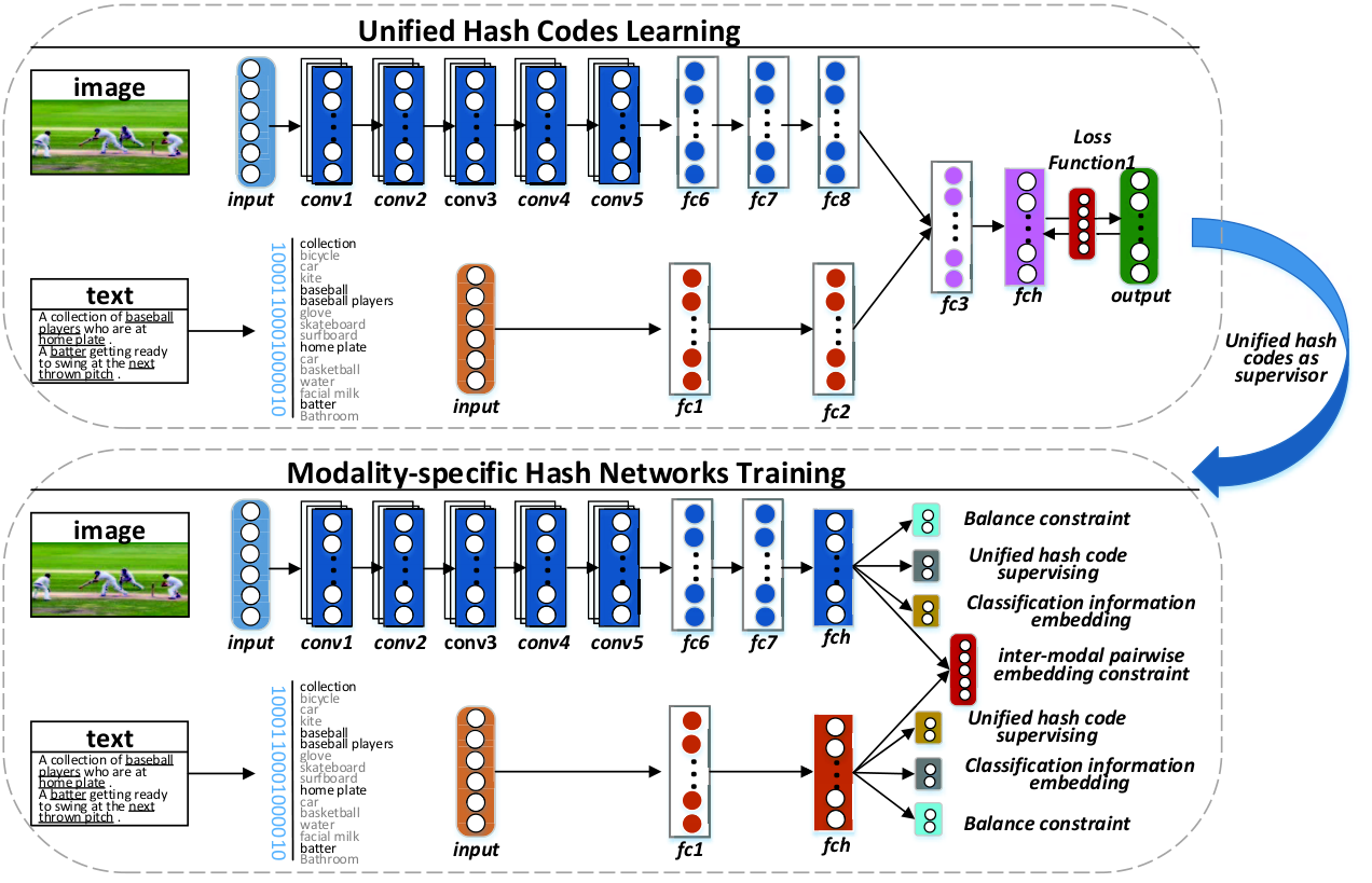
The basic deep framework of FDCH model is illustrated in Figure 1. It consists of two components:

Unified hash codes learning: There are three networks involved in this component: image network, text network and fusion network. For the design of the image network, we use the CNN-F network in [25]. The original CNN-F model consists of eight layers: five convolutional layers $(conv1-conv5)$ and three fully-connected layers $(fc6-fc8)$. For the text modality, we first represent each text sample as a vector with Bag-of-Word (BOW) representation, and then input the BOW vector into the text network with two fully-connected layers. In particular, the number of hidden nodes in the last fully-connected layer of the image and text network should be consistent. For fusion network combines the outputs of image and text networks in pairs, it consists of two fully-connected layers. To obtain the unified hash codes, the second layer is designed as a hash layer $fch$ (with $k$ hidden nodes), and the activation function is an identity function.

Modality-specific hash networks training: In order to learn the hash functions for encoding out-of-sample queries, we redesign the image and text networks for training modality-specific hash networks. In this component, the last fully-connected layers of the image and text networks are replaced with the hash layer $fch$ (with $k$ hidden nodes), the identity function is used as the activation function, the rest of the settings are the same as the above step.

Assume cross-modal dataset is $O=\left\{{\left.{{o_{i}}}\right\}}\right._{i=1}^{n}$ containing $n$ training sample pairs, where ${o_{i}}=\left({{v_{i}},{t_{i}},{y_{i}}}\right)$. Correspondingly, $V=\left[{{v_{1}},...,{v_{n}}}\right]\in{\mathbb{R}^{{d_{v}}\times n}}$ and $T=\left[{{t_{1}},...,{t_{n}}}\right]\in{\mathbb{R}^{{d_{t}}\times n}}$ are image and text features, respectively. Let $Y=\left[{{y_{1}},...,{y_{n}}}\right]\in{\mathbb{R}^{{c}\times n}}$ denote label matrix for all training samples, and if $o_{i}$ belongs to the $j$-th class ${y_{ji}}=1$, otherwise ${y_{ji}}=0$. Given the label information, the pair-wise similarity matrix is defined as $S=\left\{{\left.{{s_{ij}}}\right\}}\right.$, where ${s_{ij}}=1$ when ${o_{i}}$ is semantically similar to ${o_{j}}$, otherwise ${s_{ij}}=0$. For multi-label datasets, we define ${s_{ij}}=1$ if ${o_{i}}$ and ${o_{j}}$ have at least one same label, otherwise ${s_{ij}}=0$.

FDCH aims to learn compact $k$-bit binary code for each instance, and $B\in{\left\{{-1,1}\right\}^{k\times n}}$ is unified hash code matrix with the $i$-th column ${b_{i}}\in{\left\{{-1,1}\right\}^{k}}$. For two binary codes ${b_{i}}$ and ${b_{j}}$, the relationship between their Hamming distances $di{s_{H}}\left({{b_{i}},{b_{j}}}\right)$ for evaluating similarity and their inner product $\left\langle{{b_{i}},{b_{j}}}\right\rangle$ is formulated as follows: $di{s_{H}}\left({{b_{i}},{b_{j}}}\right)=\frac{1}{2}\left({k-\left\langle{{b_{i}},{b_{j}}}\right\rangle}\right)$. Obviously, two binary codes with larger inner products have smaller Hamming distances. Therefore, we can use the inner product of different binary codes to quantify their similarity. Given pair-wise similarity matrix $S=\left\{{\left.{{s_{ij}}}\right\}}\right.$, the probability of ${s_{ij}}$ under the condition $B$ is defined as:

where $\sigma\left({{\Psi_{ij}}}\right)=\frac{1}{{1+{e^{-{\Psi_{ij}}}}}}$ is a sigmoid function, and ${\Psi_{ij}}=\frac{1}{2}\left\langle{{b_{i}},{b_{j}}}\right\rangle=\frac{1}{2}b_{i}^{T}{b_{j}}$. Eq.(1) shows that samples with larger inner products should have higher probability of being similar, so it can measure the similarity of hash codes.

Let $\mathop{f}\limits^{\sim}\left({V;{\theta_{v}}}\right)$ denote the learned feature representation corresponding to the output of the image network, $\mathop{g}\limits^{\sim}\left({T;{\theta_{t}}}\right)$ denote the learned text feature corresponding to the output of the text network. Given the output of the image and text networks, we can combine them with the nonlinear activation (tanh) function $t\left(\cdot\right)$ to get the input $Z=t\left({}\right.\mathop{f}\limits^{\sim}\left({V;{\theta_{v}}}\right)+\mathop{g}\limits^{\sim}\left({T;{\theta_{t}}}\right)\left.{}\right)$ of the fusion network. Further, we define the output of the fusion network for all training as $H=h\left({Z;{\theta_{z}}}\right)\in{\mathbb{R}^{K\times n}}$. By jointly training the image network, text network and fusion network, our method nonlinearly transforms the paired training samples into powerful unified hash codes in this step.

Combining with the above analysis of similarity measure, the objective function for learning the unified hash codes can be defined as follows

where the first term is a negative log likelihood function $-\sum\limits_{{s_{ij}}\in S}{\log p\left({{s_{ij}}|B}\right)}=-\sum\limits_{{s_{ij}}\in S}{\left({{s_{ij}}{\Phi_{ij}}-\log\left({1+{e^{{\Phi_{ij}}}}}\right)}\right)}$, and ${\Phi_{ij}}=\frac{1}{2}H_{*i}^{T}{H_{*j}}$. Besides, $\lambda$ and $\eta$ are hyper-parameters. The first term is a pair-wise embedding constraint to preserve the semantic similarities in $S$. By minimizing the negative log likelihood function, it makes the similarity (inner product) between two similar samples as large as possible, and the similarity between dissimilar samples as small as possible. The second term minimizes the loss between outputs of the fusion network and binary hash codes, so that the learned unified hash codes can preserve the nonlinear correlations among training samples. The third term is a balance constraint to maximize the information of each hash bit. It requires each bit to have an equal opportunity to be coded to 1 or -1 for all training samples.

The optimization problem in Eq.(2) can be solved by using the iterative update strategy. Specifically, we can learn one variable while fix other variables alternatively. We learn unified hash codes $B$ and network parameters $\theta=\left\{{{\theta_{v}},{\theta_{t}},{\theta_{z}}}\right\}$ as follows.

Update $\theta$, with $B$ fixed: we adopt the mini-batch Stochastic Gradient Descent (SGD) to learn $\theta=\left\{{{\theta_{v}},{\theta_{t}},{\theta_{z}}}\right\}$. We first compute the gradient of the loss function in Eq.(2)

Then we can obtain the gradients of each layer through the chain rule and update the parameters $\theta$ by Back Propagation (BP) [26] algorithm.

Update $B$, with $\theta$ fixed: In the optimization process, we keep the discrete nature of unified hash codes $B$. When $\theta$ is fixed, we can obtain the following formulation

The hash codes ${B_{ij}}$ can be solved as

We have learned powerful unified hash codes for all training sample pairs through above steps. In this section, we train the image network $f\left({V;{\theta_{v}}}\right)$ and text network $g\left({T;{\theta_{t}}}\right)$ to obtain corresponding hash functions ${h^{v}}\left(\cdot\right)$ and ${h^{t}}\left(\cdot\right)$ for encoding out-of-sample queries.

Firstly, we adopt the inter-modal pair-wise embedding constraint preserve the cross-modal similarity between the outputs from image network hash and text hash network.

where ${\Theta_{ij}}=F_{*i}^{T}{G_{*j}}$.

Obviously, by optimizing the negative log likelihood of the pair-wise similarity $S$, the Hamming distance between two semantically similar samples can be reduced, while increasing the Hamming distance between semantically dissimilar samples.

Then, we use the high-quality hash codes learned before to supervise the training of modality-specific hash networks. By minimizing the loss function below, the nonlinear correlations embedded in $B$ are transmitted to hash networks $f\left({V;{\theta_{v}}}\right)$ and $g\left({T;{\theta_{t}}}\right)$. At the same time, the outputs of the last fully connected layer for two hash networks are forced to be close to the binary code.

Although the pair-wise similarity information in Eq.(6) and the unified hash codes containing the nonlinear correlation in Eq.(7) have been used to learn the hash functions, the semantic label information is not fully exploited.

Next, we model the relationship between the hash networks and the label information. The trained hash networks of image and text are expected to be optimal for classification. We use the label information directly by linearly mapping it into modality-specific networks as follows

where $W_{1}^{\texttt{T}}\in{\mathbb{R}^{k\times c}}$ and $W_{2}^{\texttt{T}}\in{\mathbb{R}^{k\times c}}$ are mapping matrices corresponding to image and text modalities, respectively.

Finally, we add the following balance constraints to maximize the information of each bit.

Based on the analysis of the above four terms, the overall objective function is rewritten as follows

where $\gamma$, $\beta$ and $\alpha$ are hyper-parameters to balance the importance of each terms.

Similarly, for the optimization problem of Eq.(10), we can also solve it through the alternate learning strategy, which learns one parameter by fixing others. The process of alternately learning parameters $\theta_{v}$, $\theta_{t}$, $W_{1}$ and $W_{2}$ is as follows.

Update $\theta_{v}$, with $\theta_{t}$, $W_{1}$ and $W_{2}$ fixed: The mini-batch SGD with BP algorithm is used to learn parameter $\theta_{v}$. For each instance ${{v_{i}}}$, we first derive the gradient of the loss function as follow

Then we can obtain the gradients of each layer through the chain rule and update the parameters $\theta_{v}$ by BP algorithm.

Update $\theta_{t}$, with $\theta_{v}$, $W_{1}$ and $W_{2}$ fixed: Similarly, we learn parameter $\theta_{t}$ through the mini-batch SGD with BP algorithm. For each instance ${{v_{t}}}$, we compute the gradient of the loss function as follow

Then we can obtain the gradients of each layer through the chain rule and update the parameters $\theta_{t}$ by BP algorithm.

Update $W_{1}$, with $\theta_{v}$, $\theta_{t}$ and $W_{2}$ fixed: It is easy to solve parameter $W_{1}$ by the regularized least squares problem. We can get the following closed-form solution

Update $W_{2}$, with $\theta_{v}$, $\theta_{t}$ and $W_{1}$ fixed: The parameter $W_{2}$ can also be solved by the regularized least squares problem. It has a closed-form solution as follow:

For a new query that is out of the retrieval database, we can easily obtain its hash code as long as one of its modalities is available. Specifically, given a query instance ${v_{q}}$ from the image modality, we use forward propagation of the image network to generate the hash code as follows:

Similarly, if a instance only has the text modality ${t_{q}}$, we can also use the text network to generate its hash code as:

MIRFLICKR-25K [27] consists of 25,000 instances collected from Flickr website. In experiments, we select instances with at least 20 labels, which has 20,015 image-text pairs. Here, each textual modality is represented as a 1386-dimensional BoW vector. For image modality, we directly use raw pixels as input.

NUS-WIDE [28] is a real-world web image dataset containing 269,648 instances. In the experiment, we select the 10 most frequent concepts to construct a subset with 186,577 image-text pairs. For each image-text pair, the textual modality is represented by 1000-dimensional BoW vector, and the image modality directly uses the raw pixels as input.

In experiments, we randomly sample 2,000 instances as query and the rest as database (retrieval set). To reduce computational cost, similar to [18], we randomly sample 5,000 instances from the database for training. After completing the training, we binarize the database samples into the hash codes and perform cross-modal retrieval.

Baselines: In experiments, we compare our FDCH with six state-of-the-art cross-modal hashing methods. They can be divided into two categories: LSSH [15], CMFH [11] and DCH [12] are supervised methods; SCM [13], SePH_km [14] and DCMH [17] are unsupervised methods. For fair comparison, at the $fc7$ from the initial CNN-F network used by our method, we extracted the CNN feature for the shallowed baselines.

Implemental Details: Our FDCH is implemented under the MatConvNet framework. For image network, we initialize the first seven layers using the CNN-F network pre-trained on the ImageNet dataset. All parameters for other deep neural networks in the FDCH model are randomly initialized. For the text network with two fully-connected layers, we set the dimension as $[8192\rightarrow 2500]$ on the MIRFLICKR-25K, and on the NUS-WIDE we set the dimension as $[8192\rightarrow 1000]$ for 16 bits, and set to $[8192\rightarrow 600]$ for 32 and 64 bits. For the fusion network which combines the outputs of image and text networks in pairs, we set the dimension of its fully-connected layers as $[4096\rightarrow k]$ on all datasets.

Hamming Ranking [17]: Table 1 shows the mAP scores of our FDCH and the compared methods with CNN-F features on MIRFLICKR-25K and NUS-WIDE, respectively. In the cross-modal retrieval task, LSSH, CMFH, SePH_km and our FDCH both learn the unified hash codes. As can be seen from Table 1, our method achieves the best performance for two different retrieval tasks on MIRFLICKR-25K. This is because our approach can effectively capture the correlation of multi-modal data through the nonlinear transformation from the fusion network. On the NUS-WIDE with complex semantic content, our FDCH also obtains superior performance compared to other methods, as shown in Table 1. The results demonstrate that FDCH can fully exploit the label information to learn more discriminative hash code.

Hash Lookup [17]: Figure 2 and 3 show the precision-recall curves by Hash Lookup. We plot the precision-recall curve by varying the Hamming radius from 0 to $k$ with a step size of 1. Figure 2 presents the precision-recall curves with 32 and 64 code lengths for different retrieval tasks on MIRFLICKR-25K. The precision-recall curves on NUS-WIDE are shown in Figure 3. It can be seen that the performance of our FDCH is significantly better than baselines.

Further, we design two variants of our method to evaluate the performance. FDCH-I ignores the classification information embedded in the modality-specific network. FDCH-II removes the pair-wise similarity constraint when training modality-specific hash network. Table 2 shows that the mAP scores of these variants are degraded. The results verify that it is effective to simultaneously embed pair-wise similarity and classification information in modality-specific network under one stream framework.

References

- [1] L. Zhu, Z. Huang, X. Chang, J. Song, and H. T. Shen, “Exploring consistent preferences: discrete hashing with pair-exemplar for scalable landmark search,” in MM, 2017, pp. 726–734.
- [2] Y. Cao, M. Long, J. Wang, and S. Liu, “Collective deep quantization for efficient cross-modal retrieval,” in AAAI, 2017, pp. 3974–3980.
- [3] Lei Zhu, Zi Huang, Xiaobai Liu, Xiangnan He, Jiande Sun, and Xiaofang Zhou, “Discrete multimodal hashing with canonical views for robust mobile landmark search,” TMM, vol. 19, no. 9, pp. 2066–2079, 2017.
- [4] L. Xie, J. Shen, J. Han, L. Zhu, and L. Shao, “Dynamic multi-view hashing for online image retrieval,” in IJCAI, 2017, pp. 3133–3139.
- [5] J. Wang, T. Zhang, J. Song, N. Sebe, and H. T. Shen, “A survey on learning to hash,” TPAMI, vol. 40, no. 4, pp. 769–790, 2018.
- [6] Lei Zhu, Jialie Shen, Liang Xie, and Zhiyong Cheng, “Unsupervised visual hashing with semantic assistant for content-based image retrieval,” TKDE, vol. 29, no. 2, pp. 472–486, 2017.
- [7] Lei Zhu, Zi Huang, Zhihui Li, Liang Xie, and Heng Tao Shen, “Exploring auxiliary context: Discrete semantic transfer hashing for scalable image retrieval,” TNNLS, vol. 29, no. 11, pp. 5264–5276, 2018.
- [8] L. Zhu, J. Shen, X. Liu, L. Xie, and L. Nie, “Learning compact visual representation with canonical views for robust mobile landmark search,” in IJCAI, 2016, pp. 3959–3967.
- [9] Xu Lu, Lei Zhu, Zhiyong Cheng, Jingjing Li, Xiushan Nie, and Huaxiang Zhang, “Flexible online multi-modal hashing for large-scale multimedia retrieval,” in MM, 2019, pp. 1129–1137.
- [10] Xu Lu, Lei Zhu, Zhiyong Cheng, Liqiang Nie, and Huaxiang Zhang, “Online multi-modal hashing with dynamic query-adaption,” in SIGIR, 2019, pp. 715–724.
- [11] G. Ding, Y. Guo, J. Zhou, and Y. Gao, “Large-scale cross-modality search via collective matrix factorization hashing,” TIP, vol. 25, no. 11, pp. 5427–5440, 2016.
- [12] X. Xu, F. Shen, Y. Yang, H. T. Shen, and X. Li, “Learning discriminative binary codes for large-scale cross-modal retrieval,” TIP, vol. 26, no. 5, pp. 2494–2507, 2017.
- [13] D. Zhang and W. J. Li, “Large-scale supervised multimodal hashing with semantic correlation maximization,” in AAAI, 2014, pp. 2177–2183.
- [14] Z. Lin, G. Ding, J. Han, and J. Wang, “Cross-view retrieval via probability-based semantics-preserving hashing,” TCYB, vol. 47, no. 12, pp. 4342–4355, 2017.
- [15] J. Zhou, G. Ding, and Y. Guo, “Latent semantic sparse hashing for cross-modal similarity search,” in SIGIR, 2014, pp. 415–424.
- [16] L. Xie, J. Shen, and L. Zhu, “Online cross-modal hashing for web image retrieval,” in AAAI, 2016, pp. 294–300.
- [17] Q. Y. Jiang and W. J. Li, “Deep cross-modal hashing,” in CVPR, 2017, pp. 3270–3278.
- [18] E. Yang, C. Deng, W. Liu, X. Liu, D. Tao, and X. Gao, “Pairwise relationship guided deep hashing for cross-modal retrieval.,” in AAAI, 2017, pp. 1618–1625.
- [19] V. E. Liong, J. Lu, Y. P. Tan, and J. Zhou, “Cross-modal deep variational hashing,” in ICCV, 2017, pp. 4097–4105.
- [20] F. Shen, W. Liu, S. Zhang, Y. Yang, and H. T. Shen, “Learning binary codes for maximum inner product search,” in ICCV, 2015, pp. 4148–4156.
- [21] Xingbo Liu, Xiushan Nie, Wenjun Zeng, Chaoran Cui, Lei Zhu, and Yilong Yin, “Fast discrete cross-modal hashing with regressing from semantic labels,” in MM, 2018, pp. 1662–1669.
- [22] Xu Lu, Lei Zhu, Zhiyong Cheng, Xuemeng Song, and Huaxiang Zhang, “Efficient discrete latent semantic hashing for scalable cross-modal retrieval,” Signal Processsing, vol. 154, pp. 217–231, 2019.
- [23] J. Song, Y. Yang, Y. Yang, Z. Huang, and H. T. Shen, “Inter-media hashing for large-scale retrieval from heterogeneous data sources,” in SIGMOD, 2013, pp. 785–796.
- [24] X. Zhu, Z. Huang, H. T. Shen, and X. Zhao, “Linear cross-modal hashing for efficient multimedia search,” in MM, 2013, pp. 143–152.
- [25] K. Chatfield, K. Simonyan, A. Vedaldi, and A. Zisserman, “Return of the devil in the details: Delving deep into convolutional nets,” in BMVC, 2014.
- [26] G. E. Hinton and R. R. Salakhutdinov, “Reducing the dimensionality of data with neural networks,” science, vol. 313, no. 5786, pp. 504–507, 2006.
- [27] M. J. Huiskes and M. S. Lew, “The mir flickr retrieval evaluation,” in MM, 2008, pp. 39–43.
- [28] T. S. Chua, J. Tang, R. Hong, H. Li, Z. Luo, and Y. Zheng, “Nus-wide:a real-world web image database from national university of singapore,” in CIVR, 2009, pp. 1–9.