Variational and Parquet-diagram theory for strongly correlated normal and superfluid systems
Abstract
We develop the variational and correlated basis functions/parquet-diagram theory of strongly interacting normal and superfluid systems. The first part of this contribution is devoted to highlight the connections between the Euler equations for the Jastrow-Feenberg wave function on the one hand side, and the ring, ladder, and self-energy diagrams of parquet-diagram theory on the other side. We will show that these subsets of Feynman diagrams are contained, in a local approximation, in the variational wave function.
In the second part of this work, we derive the fully optimized Fermi-Hypernetted Chain (FHNC-EL) equations for a superfluid system. Close examination of the procedure reveals that the naïve application of these equations exhibits spurious unphysical properties for even an infinitesimal superfluid gap. We will conclude that it is essential to go beyond the usual Jastrow-Feenberg approximation and to include the exact particle-hole propagator to guarantee a physically meaningful theory and the correct stability range.
We will then implement this method and apply it to neutron matter and low density Fermi liquids interacting via the Lennard-Jones model interaction and the Pöschl-Teller interaction. While the quantitative changes in the magnitude of the superfluid gap are relatively small, we see a significant difference between applications for neutron matter and the Lennard-Jones and Pöschl-Teller systems. Despite the fact that the gap in neutron matter can be as large as half the Fermi energy, the corrections to the gap are relatively small. In the Lennard-Jones and Pöschl-Teller models, the most visible consequence of the self-consistent calculation is the change in stability range of the system.
1 Introduction
The repertoire of methods for the quantitative microscopic description of normal quantum many-body systems has condensed, over the past few decades, to a relatively small number of techniques. These can be roughly classified on the one hand side as various shades of large-scale numerical simulation methods and, on the other hand, diagrammatic approaches summing, in some approximation, the parquet class of Feynman diagrams. Numerical simulations are capable of high precision but are computationally demanding and limited to relatively simple Hamiltonians and mostly ground state properties. They also need the physical intuition of the user about the possible state of the system. Semi-analytic, diagrammatic approaches lead to a better understanding of the underlying physical mechanisms, but have limited accuracy due to some necessary approximations. These diagrammatic approaches are versions of Green’s function methods [1], Coupled Cluster theory [2], and variational methods [3]. The interconnections between the various methods are well understood for Bose systems [4, 5]; the level and the details of implementation for different systems varies, however, vastly.
For normal systems, Jackson et al. make compelling arguments [4] that the summation of the so-called parquet diagrams is a minimum requirement for a microscopic treatment of the many-body problem that that treats both the short-ranged structure and the long-wavelengths excitations on equal footings. We will review these arguments further below. There are presently basically two theoretical approaches that have the diagrammatic completeness of the parquet diagrams, these are the Jastrow-Feenberg variational method [3] and the local parquet-diagram summation of Refs. 4 and 6. These methods have led, for boson systems, to exactly the same equations.
The situation is also intuitively clear for fermions, although technically more complicated due to the multitude of exchange diagrams generated by the antisymmetry of the fermion wave function, Unfortunately the fermion version [7] has so far not led to practical applications.
Among the many-body methods that sum, in some approximation, the parquet class of diagrams, the Jastrow-Feenberg method has been developed farthest. Both, local parquet theory and the Jastrow-Feenberg method are “robust” in the sense that exactly the same equations can be used for very different interactions like electrons, nucleons, and quantum fluids. Coupled Cluster theory [2] has also been very successful for electrons [8, 9] and nuclear systems [10, 11, 12] but it requires different truncation schemes for these two classes of many-body system. It lacks, therefore, the robustness of the Jastrow-Feenberg method. It was also less successful in predicting the ground state properties of the helium fluids. For bosons, a version of coupled cluster theory - the so-called “super-SUB-2” approximation has been developed [5] that is equivalent to the local parquet or Jastrow-Feenberg theory.
All of the above statements refer to normal systems. However, pairing phenomena are ubiquitous in the physics of many-body systems. Sixty years ago, the proof of the Cooper theorem [13, 14] provided the key to understanding the pairing phenomenon in interacting many-fermion systems, triggering the creation of the BCS theory of electronic superconductivity. It was quickly understood [15] that this work also has significant implications for nuclear phenomena, basically explaining the energy gap between the ground state and the first excited state for certain classes of nuclei. Since that landmark development, the basic paradigm of BCS theory has been extended to diverse fermionic systems with considerable success. We refer to two recent excellent review articles [16, 17] for a very complete account of the present situation and a comprehensive survey of the relevant literature. The work to be presented in this paper is meant to be complementary to these papers. We will, as far as justifiable, avoid overlaps. Rather, we shall focus on the technical aspects of many-body theory and spend very little space reviewing and comparing specific calculations.
A theory for superfluid many-body systems of the same diagrammatic completeness that was achieved for normal systems is presently unavailable, although specific partial summations of the perturbation series have been carried out [18, 19, 20, 21]. A version of Coupled Cluster theory for BCS-type wave functions has also been developed [22].
In systems where the pairing is due to the underlying many-body Hamiltonian, one often relies on effective interaction approximations which have the useful feature to permit the examination of mechanism and dependencies, but come with all the uncertainties involved in constructing effective interactions.
One of the intentions of our paper is therefore to develop a theory superfluid systems that is diagrammatically, as far as justified by the problems at hand, equivalent to the Jastrow-Feenberg or parquet theory for normal systems.
Our paper is organized as follows: In the following section, we will first give a pedagogical review of the motivations behind the correlated wave function method and the parquet-diagram theory. We will begin with the optimized hypernetted chain (HNC-EL) method for bosons which has proven to be the preferred systematic method of summing infinite classes of cluster diagrams.
As mentioned above, the boson version of the theory is identical to the summation of local parquet diagrams or to a specific version of coupled cluster theory. A priori, all two-particle vertices in a Feynman-diagram based theory are functions of four energy/momentum variables. Energy and momentum conservation and isotropy reduce that to ten variables which is still too much for diagram summation methods. Local parquet theory then introduces specific approximations to make all vertices functions of the momentum transfer only, and derives a procedure to replace the energy dependence by an average energy.
The situation is much more complicated for fermions for two reasons: One is that the antisymmetry requirement for the wave function leads to a multitude of exchange diagrams, the other is that the Fermi sea provides a natural frame of reference, whereas the Jastrow-Feenberg theory makes the approximation that all correlations depend only on the distance between particles. That requires futher approximations.
We will here examine what approximations must be made to go from a specific set of Feynman diagrams to a corresponding set of Jastrow-Feenberg diagrams. It will turn out that exactly the same procedure of defining an average energy that has been established for Bose systems [4] can be carried over to Fermi systems. The existence of a preferred frame of reference will require an additional Fermi-sea averaging procedure to generate vertices that depend only on the momentum transfer. We will see that exactly the same procedures for defining an average energy and an average momentum apply in the three channels, particle-hole, particle-particle, and single-particle propagators.
Realizing the relevant correspondences we will be led to formulate a hybrid theory that has the same diagrammatic content as the variational theory but avoids some important approximations.
We then develop the generalization of the Jastrow-Feenberg method for superfluids. We derive the diagrammatic expansions, carry out the FHNC summations for a correlated superfluid state, and derive the Euler equation for optimizing the correlations. By examining the Euler equation, we will unveil a severe problem of the Jastrow-Feenberg wave function: We will demonstrate that the Euler equation for the pair distribution function displays spurious instabilities for net-attractive interactions, characterized by an attractive Landau parameter . We will demonstrate that these problems are caused by the so-called “collective” or “single-pole” approximation [26, 27] for the particle-hole propagator, which is implicit to the Jastrow-Feenberg wave function and will be discussed at length in Section 4. We are therefore lead to conclude that the Jastrow-Feenberg wave function for a superfluid system does not permit a sensible optimization of the pair correlations. Hence, one must go beyond the simple Jastrow-Feenberg method and to implement the correlated-basis functions (CBF) or parquet-diagram theory for superfluid states. We will show that the instabilities are then removed.
The need for developing CBF/parquet-diagram methods for the superfluid state has also a quantitative reason. We have argued – and demonstrated – many years ago that local correlations of the kind (2.3) are inadequate to deal with pairing phenomena. The qualitative explanation for that is quite simple: local correlation functions treat all particles within the Fermi sea in the same way. BCS-pairing occurs at the Fermi surface; correlations that are independent of the location of the particle within the Fermi seas should therefore be particularly poor to describe pairing phenomena. Quantitative evidence for this was provided in our neutron matter calculations of Refs. 28 and 29. This is another reason that one must go beyond the Jastrow-Feenberg theory to deal with pairing phenomena reliably.
In Secs. 6.1, 6.2, and 6.3, we apply our theoretical methods to a few physically interesting cases: model Fermi gases at low densities, and neutron matter. With that, we follow up on previous works [30, 31] which was partly motivated by the interest in the BCS-BEC crossover in cold Fermi gases (see Refs. 32 and 33 for review articles) and superfluidity in neutron matter (see Ref. 34 for a collection of review papers). We have recently examined pairing phenomena in both model Fermi systems [35] and neutron matter [36]. We extend these calculations, which have assumed a small superfluid gap and treated the BCS correlations perturbatively, within the much more advanced theory to be developed in this paper.
In applications to neutron matter, we demonstrate that the inclusion of the full superfluid propagators in both the density and the spin-channel have a rather visible consequence for the superfluid gap.
The second case to be discussed are many-particle systems interacting via a family of Lennard-Jones model interaction. The attractive Lennard-Jones liquid has a more interesting phase diagram than neutron matter since it can have two spinodal points at which the speed of sound vanishes. One spinodal point appears at negative pressure at about 60 percent of the equilibrium density. This point can be reached by gradually lowering the density; it is characterized by the fact that the Fermi liquid Landau parameter . A second spinodal point appears at very low density when the attractive interaction begins to dominate over the Pauli pressure. The appearance of this instability is obvious from the equation of state, it has already been observed by Owen [37].
We have studied BCS pairing for the Lennard-Jones interactions extensively in Ref. 35 in an approximation that assumed that the BCS correlations are weak. Going beyond this approximation, we face the aforementioned spurious instabilities of locally correlated wave functions which have a drastic effect in the Lennard-Jones liquid: In the whole density regime where the weakly coupled theory predicted a superfluid transition, FHNC-EL equations for local correlations have no physically acceptable solutions. We solve this problem by including the correct superfluid particle-hole propagator which has a quite visible quantitative effect on both the phase diagram and pairing properties.
Computations in the vicinity of the spinodal points become very demanding since the correlations become very long-ranged. In Ref. 35, we have observed that it is rather easy to come close to the upper spinodal point. However, getting close to the lower spinodal point turned out to be impossible since the solutions to the FHNC-EL equations diverge already a distance from the limit . This divergence was identified as a divergence of the in-medium scattering length. We find exactly the same property in our much more advanced calculations to be presented in this paper. In fact, our inclusion of exchange diagrams, which improves the predictions of the Fermi-liquid parameter significantly, hardly changes the location of the instability.
Computations for the purely attractive Pöschl-Teller potential, which has due to the absence of a repulsive hard core no stable high-density phase and only the lower spinodal point confirm our conclusions.
We conclude this paper with a brief summary of our results.
2 Motivation: Variational and local parquet theory for bosons
2.1 Rationalization of parquet diagram summations
To describe the physics in the interaction-dominated short-distance region within diagrammatic perturbation theory, short-ranged correlations must be dealt with properly. These are treated, in perturbation theory, by summing the ladder diagrams which determine, among others, the pair distribution function at small distances. The description of generally long-ranged effects, in particular phonons or plasmons and the behavior of the static structure function at long wavelengths , requires the summation of chain diagrams. The simultaneously correct treatment of both short- and long-ranged effects requires, therefore, the self-consistent summation of ring- and ladder-diagrams which defines the set of parquet diagrams [4, 6, 38].
The resulting two-body vertices are still functions of three independent four-momenta. To make execution of the theory practical, approximations must be made. Local parquet theory localizes the vertices by choosing an average energy such that the contribution to the pair distribution of the full vertex is the same as the that of the localized one. That way, the iterative procedure is, in every step, connected to a physical observable. Moreover, we shall see below that the pair distribution function can indeed be considered the only necessary independent variable that determines the properties of the system.
Carrying out this procedure for bosons, it turns out that one arrives at a set of equations that had been known for many years [3, 39, 40, 41], namely the HNC-EL equations [6] (dubbed “Paired-Phonon Analysis at that time) and the HNC-EL energy functional [38]. In fact, the analogy goes farther in the sense that the inclusion of the leading non-parquet diagrams [42] is the same as the inclusion of optimized three-body correlations in the wave function (2.3) [43].
The situation is more complicated for fermions, mostly due to the multitude of additional diagrams. Of course, since the correspondence between parquet diagrams and the HNC-EL method is clear for bosons, a similar correspondence should be expected for fermions.
In the nexy section we shall demonstrate the analogy between fermion parquet theory and FHNC-EL for important classes of diagrams, namely the ring- and ladder-diagrams. This is the essence of the simplest version of FHNC-EL, referred to FHNC-EL//0 [44]. More complete implementations [27] also include RPA-exchange diagrams, self-energy corrections, and mixture of all of these. These versions are referred to as FHNC//n where n is the level of higher-order exchange diagrams retained. As we shall see, the prescription of making all vertices energy-independent by choosing a well-defined average energy can be carried over from the boson parquet theory. The existence of a preferred reference frame, the Fermi sea, still causes the simplest vertices depend on three momenta; turning these into functions of momentum transfer will require the introduction of an additional specific averaging procedure of single-particle energies over the occupied states in the Fermi sea.
Both of these localizing procedures might seem ad-hoc from the point of view of conventional perturbation theory, and without further consideration other procedures might look equally well justified. They are rationalized by the fact that these localization prescriptions lead to the Jastrow-Feenberg wave function (2.3). The optimization prescription (2.8) makes sure that one has, that way, constructed the best wave function that can be represented in terms of local functions. In fact, a generalization of the Hohenberg-Kohn theorem to two-body functions [45, 46] shows that the pair distribution is indeed quite generally defined by a variational problem.
The Jastrow-Feenberg wave function is known to reproduce the properties of both helium fluids with better than 90 percent accuracy [47]; below about 25 percent of the helium saturation density the accuracy of the FHNC//0 approximation is better than 1 percent, and Coulomb systems, both bosons [43] and fermions [48] are generally reproduced at the percent level or better.
2.2 Hypernetted Chain and Euler equations
We choose the Jastrow-Feenberg approach here to derive what we shall refer to as “generic” many-body method because it requires relatively little formal input. It is suitable for a non-relativistic many-body Hamiltonian
| (2.1) |
The method starts with an ansatz for the -body wave function,
| (2.2) | |||||
| (2.3) |
where is the normalization constant. Here is a model state, which is normally a Slater determinant for normal Fermi systems, and is an -body correlation operator. The explicit reference to the particle number will be necessary later when we generalize the method to BCS states, we shall omit it from now on for the normal system which has a fixed particle number.
When truncated at the two-body term , Eq. (2.3) defines the standard Jastrow theory. Historically [49] the theory was developed as a “quick and dirty” way to deal with the strong, short-ranged forces prevalent in nuclei. The task of the function is to bend the wave function to zero inside the regime of the repulsive hard core. The energy expectation value
| (2.4) |
and other physically interesting quantities like the pair density
| (2.5) |
the pair distribution function
| (2.6) |
and the static structure function
| (2.7) |
are then calculated by cluster expansion and resummation techniques. We will deal in this paper exclusively with translationally invariant and isotropic systems, hence .
A typical situation is seen in Fig. 1 where we examine the example of an interaction with a strong repulsive core and an attractive well. We show correlation and distribution functions for that interaction. The specific example is for one of the Lennard-Jones models to be discussed in Section 6.2. At higher densities, the pair distribution function begins to develop oscillations typical for strong short-ranged order. The correlation function and the “dressed” correlation function to be introduced in Section 3.3 describe the dynamic correlations induced by the interaction whereas the pair distribution function is determined by both dynamic and statistical correlations.

The evaluation of physical quantities for the wave function (2.3) requires approximations. It was quickly realized [3] that the hypernetted chain summation (HNC) and truncation scheme has the advantage over other integral equation techniques like Born-Green-Yvon [50] or Percus Yevick[51] that it facilitates the unconstrained functional optimization of the pair correlations by solving the Euler equation
| (2.8) |
To set the scene for the further discussions, and to demonstrate both the simplicity and the power of the method, as well as its physical content, let us first discuss the simpler case of a Bose liquid. In that case, the model state is . The HNC scheme for bosons is known from the theory of imperfect gases where the Jastrow correlation function is replaced by , being the inverse temperature [52, 54, 53]. The equations are
| (2.9) |
Above, and are the sums of “non-nodal” and “nodal” diagrams, and is the sum of “elementary” diagrams which can be expressed in terms of the pair distribution function . We define, as usual in this field, the dimensionless Fourier transform by including a density factor :
| (2.10) |
The elementary diagram contributions have to be included term by term; they change the numerical values of the results, but not the analytic structure of the equations. Three-body correlations also lead only to a modification of that term [55].
The pair correlation function can be eliminated entirely from the theory by utilizing the Jackson-Feenberg identity
| (2.11) |
For a Jastrow wave function, the second term can be written as
| (2.12) |
and, eliminating via the HNC equations (2.9), leads after a few manipulations to
| (2.13) | |||||
| (2.14) | |||||
| (2.15) | |||||
| (2.16) |
where is the kinetic energy.
It is then straightforward[39, 3, 56] to derive the Euler equation
| (2.17) |
Skipping the technical details we display the resulting equations:
| (2.18) | |||||
| (2.19) | |||||
| (2.20) |
Above,
| (2.21) |
is the contribution from elementary diagrams and, if applicable, multiparticle correlations.
A few algebraic manipulations show that the pair distribution function satisfies the coordinate-space equation [56]
| (2.22) |
Eq. (2.18) recognized as a Bogoliubov equation in terms of an effective “particle-hole” interaction . Likewise, Eq. (2.22) is recognized as the Bethe-Goldstone equation in terms of the interaction . This observation led Sim, Woo, and Buchler [40] to the conclusion that “it appears that the optimized Jastrow function is capable of summing all rings and ladders, and partially all other diagrams, to infinite order”.
The results (2.18) and (2.22) also substantiates the assertion made above that the HNC summation scheme is the method of choice over alternatives because it facilitates the optimization of the correlations: No matter which approximation we choose for the elementary diagrams, and whether we include higher order correlation functions, the only thing that changes is the correction term , but the structure of the equation remains the same.
2.3 Pair density functional theory: The view from the top
We have already commented in Section 2.2 that the pair correlation function can be eliminated entirely from energy expression which is then formulated entirely in terms of the physical observable . It is therefore natural to ask whether a general minimum principle exists for the pair distribution function. Effectively, we are looking for a two-body version of the Hohenberg-Kohn [57, 58] theorem.
Let us write the energy per particle as
| (2.23) |
where
| (2.24) |
is the potential energy, and the kinetic energy whose form is yet unspecified.
Following the line of arguments leading to the Hohenberg-Kohn theorem for the one-body density, three statements can be made:
- (1)
The kinetic energy depends only on and not on .
- (2)
Assuming that the interaction goes to zero at large distances, there is a bijective mapping between and .
- (3)
The total energy has a minimum equal to the ground state energy at the physical ground state distribution function, in other words the ground state distribution function can be obtained by functionally minimizing the energy (2.23) with respect to the distribution function .
The proof parallels exactly the proof of the original Kohn-Hohenberg theorem and does not need to be repeated here.
Let us assume now that we have a variational problem of the form (2.17) with an energy functional (2.23), (2.24). We then can calculate the pair distribution function (or the static structure function) for any potential with .
Replacing, in Eq. (2.24) by and differentiating with respect to gives
| (2.25) |
The second term in Eq. (2.25) vanishes, we can therefore recover the energy by coupling constant integration,
| (2.26) |
where is the pair distribution function calculated for a potential strength , and is the energy of the non-interacting system which is zero for bosons, and equal to the energy of the non-interacting Fermi gas for fermions.
In Eq. (2.26) we recover, of course, the Hellmann-Feynman theorem [59, 60] which was originally proven for the exact ground state. The above derivation [38] shows that the theorem is true not only for the exact ground state, but also for any approximate energy functional, as long as the pair distribution function is obtained by minimizing that functional.
Evidently, the above statement is much more general than the optimization condition (2.17) for the Jastrow–Feenberg wave function because it defines a whole class of many–body theories which can be characterized by the central role of the pair distribution function. To summarize, the above consideration shows that the many-body theory of strongly interacting systems can indeed quite generally be formulated in terms of a local two-body quantity. This provides, similar to the tremendously successful density functional theory of inhomogeneous electron systems, a significant simplification compared to Greens’s function theories.
The above analysis is evidently independent of the statistics, it applies equally well for bosons and fermions.
So far, our considerations were entirely parallel to conventional density functional theory; the energy functional is still unspecified. The next step is therefore the construction of a “pair density functional”. Unlike the conventional density functional of inhomogeneous electron systems, some exact features of the pair distribution function are known that can be used for the construction of a pair-density functional (2.23).
- 1.
The static structure function is related to the density–density response function through
(2.27) Assuming, for example, an RPA form of the density-density response function defines a local “particle–hole interaction” by an RPA formula
(2.28) where is the Lindhard function.
- 2.
The short-ranged structure of the pair distribution function is determined by a Bethe-Goldstone equation in terms of a yet unspecified particle–particle interaction We can assume that, for short, distances, is dominated by the bare interaction , i.e. we can write
- 3.
We require that and are consistent in the sense that they are related by Eq. (2.7).
For bosons, all the calculations can be carried out analytically. In the absence of Pauli operators, the Bethe Gladstone equation is simply a zero-energy Schrödinger equation
| (2.29) |
Just as we can think of Eqs. (2.27) and (2.28) as a definition of in terms of , we can think of Eq. (2.29) as a definition of in terms of .
For bosons we have
| (2.30) |
Then, the frequency integration (2.27) can be carried out analytically and leads to the familiar Bogoliubov formula (2.18). Simply manipulating Eqs. (2.27)-(2.30) then leads to the HNC-EL equations (2.18)-(2.20), (2.22) [45]. The only undetermined quantity is the correction which is, in HNC-EL, determined by the elementary diagrams and multiparticle correlation functions retained; in local parquet theory it is the set of diagrams that are both particle-particle and particle-hole irreducible [42].
To summarize, the HNC-EL theory supplements the variational prescription following from the Hohenberg-Kohn theorem for the pair distribution function by the requirement that function satisfies both, a Bethe-Goldstone equation and an RPA equation. Hence, we shall refer to the equations as generic equations because they can be obtained without ever mentioning a Jastrow-Feenberg function.
2.4 Stability and Consistency
A condition for the existence of solutions of the Euler equation is that the term under the square-root in Eq. (2.18) is positive. We must identify the long-wavelength limit with the hydrodynamic speed of sound,
| (2.31) |
to obtain the correct long wavelength limit
| (2.32) |
An immediate consequence is that the HNC-EL or local parquet equations have no solution of the system is unstable against infinitesimal density fluctuations. This is a very desirable feature and unique to theories that have the diagrammatic completeness of the parquet theory.
Alternatively we can calculate the hydrodynamic speed of sound from the equation of state
| (2.33) |
The definitions (2.31) and (2.33) will, in any approximate theory, not be identical. In fact, it can be shown in both Jastrow-Feenberg theory [61] and in parquet-diagram theory [62] that they agree only when all diagrams and correlations to all orders are included. Turning this feature in an advantage, the comparison between the definitions (2.31) and (2.33) can serve as a convergence test of approximate evaluations. We will utilize this feature in our numerical studies below.
3 Variational and local parquet diagram theory for fermions
The Jastrow-Feenberg method for fermions has been successfully applied to the relatively simple electron liquid [63, 64, 48], nuclear systems [65] as well as highly correlated Fermi systems like 4He [55, 46] and 3He [37, 61, 27] at and finite temperatures [66, 67, 68]. The full fermion HNC equations [69, 70, 71] are significantly more complicated than the bosons equations (2.9); instead of one set of nocal, non-nodal, and elementary diagrams we have four sets. Moreover, very specific truncation schemes of exchange diagrams are necessary to permit an unconstrained optimization of the correlations [61], the above-mentioned hierarchy of FHNC//n approximations.
We have shown in recent work [72] that even the simplest version of the FHNC-EL theory reproduces the equation of state within better than one percent at densities less than 25% of the saturation density of liquid 3He. This statement applies to the energy, other quantities are, as we shall see, more senesitive to level at which the FHNC are implemented. A similar statement applies for nuclear systems [36]. It is not much more complicated to solve the full set of FHNC-EL equations, including elementary diagrams and triplet correlations [27]. The version to be presented here permits, however, a clearer identification of sets of FHNC diagrams with Feynman diagrams.
3.1 Generating functional and the generalized distribution functions
We describe in this and the following sections the basic techniques of cluster expansions and resummations for Fermi systems. The manipulations of Section 2.2 relied on the simplicity of the HNC equations (2.9) for bosons. We must now be more systematic, this is also necessary in view of the generalization to superfluid systems to be described below.
The central quantity for all derivations is the “generating function” defined as follows: Substitute in the variational wave function (2.3)
| (3.1) |
where
| (3.2) |
is the “Jackson-Feenberg effective interaction”. With this, all quantities depend on the dummy parameter . Define then the generalized normalization integral
| (3.3) |
and the generating function
| (3.4) |
The value is just the logarithm of the norm of the wave function, but evidently it is technically no more complicated to calculate than it is to calculate .
The energy expectation value may be obtained from the generating functional through
| (3.5) | |||||
Here is the kinetic energy of the non-interacting Fermi gas, and
| (3.6) |
is an energy correction in Fermi systems that will be dealt with below. Further, it is convenient to define generalized densities
| (3.7) |
The (generalized) two-body density may be derived as a variational derivative of the generating function with respect to the (generalized) pair correlation function
| (3.8) | |||||
| (3.9) |
a relation that will be particularly useful for the derivation of the Euler equations. The last expression shows that the procedure generates a which has an overall factor .
For the case , the definition (3.7) reduces to the two-body density introduced above (cf. Eq. (2.5)),
| (3.10) |
The construction of both the energy and the distribution functions via derivatives of one common generating functional is a welcome economy since it is sufficient to develop an algorithm for the calculation of ; one does not need to start over for each individual quantity of interest. For example, we can immediately write down the exact Euler equation for the pair distribution function:
| (3.11) |
where
| (3.12) |
3.2 Cluster expansions
A very straightforward technique to derive cluster expansions for the generating function and, or course, any other quantity of interest is the power-series method [71]. The method introduces a dummy parameter in the correlation operators
| (3.13) |
where and we have suppressed the parameter . One then expands the quantity of interest in a power series in , evaluated at . For example,
| (3.14) | |||||
That way, a series of cluster contributions of increasing number of factors is generated. These are best represented diagrammatically [44]:
- 1.
Each point (open dot) represents a particle coordinate .
- 2.
Each filled point (solid dot) implies the integration over the coordinate , and multiplication with a density factor , where is the normalization volume.
- 3.
Correlation line connecting the points and represent a function . These are depicted as dashed lines connecting the two points.
(3.15) - 4.
Exchange lines represent the function
(3.16) These are depicted by oriented solid line connecting the point to ,
(3.17)
We call a diagram linked if each point is connected to every other point by at least one continuous path of graphical elements. Linked diagram contributions to the generating functional are proportional to the particle number. We call diagram irreducible if it cannot be calculated as a product of two or more simpler diagrams.
The cluster expansion of the generating function is then represented in terms of all topologically distinct irreducible diagrams without external points constructed by the following rules:
- 1.
Each point is attached by at least one correlation line.
- 2.
Two points can be joined by at most one correlation line.
- 3.
Any point of a contributing diagram is joined by at most one incoming exchange line which must be accompanied by a single outgoing exchange line. Hence, exchange lines come in closed loops. For each closed loop of exchange lines there is a factor in the corresponding analytic contribution, as well as the exchange function. (Generally, the sign is displayed with the diagram, but the numerical factor is left implicit.) Here, is the degree of degeneracy of the single particle states.
The first terms in the diagrammatic expansion of the generating function are shown in Fig. 2.

The generalized pair distribution function can then be derived by the variational prescription (3.8) and the energy expectation is obtained from the general expression (3.5) as follows
- 1.
Replace, in turn, each correlation line by a line . This is what the -derivative does.
- 2.
To calculate the kinetic energy corrections replace any pair of exchange lines by a pair .
Cluster contributions for the (generalized) pair distribution function can then be generated by the prescription (3.8). Diagrammatically, the construction of amounts to the following operation on the generating function :
- 1.
Remove, in turn, each correlation line and turn its endpoints into open (“reference”) points and
- 2.
Multiply this by . This factor is needed to model the short-ranged structure of the wave function for hard-core potentials.
A few low-order diagrams contributing to the pair distribution function are shown in Fig. 3.

The figure shows the expansion of in terms of correlation and exchange lines. Two adjacent diagrams (a) and (b), (c) and (d) etc. can always be combined to obtain the form (3.9), in other words the function is represented by diagrams (a), (c), (e), etc.. This is exactly the intention of Jastrow-Feenberg theory [49, 3], namely to have the correlation function model the short-ranged structure of the wave function.
Close inspection of the individual contributions to reveals, however, a dilemma: For the stability of the system as well as for meaningful solutions of the Euler equation, it is important long ranged correlations are important, cf. Eq. (2.32). To get the correct behavior of for , the diagrams must be grouped differently. For example, diagrams (b), (h), and (k) combine to
where
| (3.18) |
is the static structure function of the non-interacting Fermi gas. Likewise, it is straightforward to show [61] that the sum of diagrams (g) and (o) as well as the sum of diagrams (d), (i), and (m) go as in the limit . The analysis can be easily extended to other, more complicated cases.
To summarize, there is no finite truncation of the expansion of the pair distribution function that is exact in both, the short-distance and the long-wavelength limit. One can deal with this situation in three ways:
- 1.
One can ignore the problem entirely and use, consistent with the original idea of Jastrow-Feenberg theory, an approximation for of the form (3.9). This is, among others, the idea of the FHNC summations of Ref. 71. One must live with the fact that the static structure function has the incorrect long-wavelength limit and the correlation functions are limited to simple parameterized forms.
- 2.
One can use different approximations for and depending on which quantity is of interest. Choosing a form for that has the exact long-wavelength behavior permits the unconstrained optimization of the pair correlations. Of course, one must then construct a pair distribution of the form (3.9).
- 3.
One must sum infinite sets of exchange diagrams or approximations thereof as was done in Ref. 27.
For the purpose of this work, we shall use the second approach because it is sufficiently accurate for all of our purposes [72, 36] and allows the most direct identification of JF diagrams with parquet diagrams.
To conclude this section, we mention another specific set of diagrams, the so–called “cyclic chain” (cc-) diagrams. These are two body diagrams that have a continuous exchange path connecting the external points. A few examples are shown in Fig. 4. We can again identify “chain” diagrams (diagrams (c), (d), and (e)), “parallel connections” (diagrams (a) and (b)) and one “elementary” diagram (diagram (f)).

The summation of these diagrams suggests the introduction of a “dressed” exchange line which is the sum of all 2-point diagrams having an exchange path connecting the two external points. The “cc” diagrams are related to self-energy corrections in perturbation theory, see Sections 3.9 and 4.4 below.
3.3 FHNC and Euler equations
We discuss here the simplest implementation of the FHNC theory that is compatible with the variational problem, called FHNC//0 approximation. The approximation keeps in only those diagrams that contain exchange loops of the form . These are, for example, the diagrams (a-g), (k) and (l) shown in Fig. 3. We must also keep in mind that a different approximation has to be used in . The implementation and relevance of higher order exchange corrections will be discussed below in Section 3.7.
In the FHNC//0 approximation, the FHNC equations are no more complicated than the Bose HNC equations (2.9):
| (3.19) | |||||
| (3.20) | |||||
| (3.21) | |||||
| (3.22) | |||||
Above, is the set of all diagrams contributing to that have no exchange lines attached to the external points. Examples are diagrams (b), (e), (f), (k) and (l) shown in Fig. 3. We need these equations to eliminate from the and to formulate the theory entirely in terms of the physically observable static structure function and derived quantities.
In this approximation, the energy correction has the form
| (3.23) |
Similar to the Bose case, the Euler equation is best formulated in momentum space. Formally, the optimization condition‘ can be written as [3]
| (3.24) |
The is generated by the -derivative technique outlined above. This amounts to
- 1.
Replace, in turn, each correlation line by . This can be done with the -derivative trick.
- 2.
To add the correction from , replace, in turn, each by .
Using the version (3.20), (3.22) of the FHNC00 equations as well as the “priming” operation outlined above we obtain
| (3.25) |
and, inserting this in the Euler equation (3.24) and solving for :
| (3.26) |
In the FHNC//0 approximation, the effective interaction is approximated by the “direct” part of the particle–hole interaction, ; we will discuss the importance to exchange corrections further below. The quantity is structurally identical to the one for bosons:
| (3.27) |
where
| (3.28) |
is the “Clark-Westhaus” effective interaction [44] and is the “induced interaction”.
| (3.29) | |||||
| (3.30) |
The second line is obtained by using Eq. (3.26) to eliminate . The Bose limit is obtained by replacing .
To derive the equation determining the short-ranged structure of the correlations, begin with Eq. (3.30) which we can write, using the Euler equation (3.26), as (cf. Eq. (2.62) of Ref. 73)
| (3.31) | |||||
Using the identity
| (3.32) |
Eq. (3.31) becomes
| (3.33) |
The right-hand side is evidently zero for bosons, and the Euler equation is a simple zero-energy Schrödinger equation where the bare interaction is supplemented by the induced potential which guarantees that the scattering length of the effective interaction is zero. This is the well-known result of Refs. 56 and 6. For fermions, the right hand side changes the short-ranged behavior of the correlation function and, hence, the short-ranged behavior of the pair distribution function . This is consistent with the prediction of the Bethe-Goldstone equation that the Pauli principle changes the short-ranged behavior of the wave function [74], see Eq. (4.22) below.
3.4 Energy
For we use Eq. (2.14) of Ref. 35 which implies the form (3.23) for the . Summarizing, we use
| (3.34) | |||||
where is the kinetic energy of the non-interacting Fermi gas, theory, and the pair distribution function is given by [35]
| (3.35) |
Above,
| (3.36) |
The two terms and are diagrammatically represented bu the 3-body and 4-body diagram shown in Fig. 5

That term is omitted the FHNC//0 approximation, it is for energy calculations in our case very small and only needed to establish the exact low density expansion of the energy in powers of to second order [75]. We found that non-universal contributions to the equation of state are overwhelming well below the densities where the second-order terms become visible. However, we will see that the correction to the particle-hole interaction originating from these diagrams is substantial even in the low-density limit.
3.5 Uniform limit approximation
The so-called “uniform limit” approximation [3] is obtained by assuming a weak, but possibly long–ranged interaction. We study this because it will permit direct contact to be made to the random phase approximation. It will also highlight a special feature for the superfluid system, see 5.5 below.
Specifically, the uniform limit approximation is valid when
note that we do not assume that or are negligible.
In the energy term in Eq. (3.34) we can use
This term is not negligible because we can write the energy contribution as
Then, the energy becomes
| (3.37) | |||||
where is the energy expectation value in Hartree-Fock approximation. The Euler equation (3.38) becomes
| (3.38) |
follows from this expression by minimization with respect to . We will see below that both (3.37) and (3.38) are is indeed approximations for of the RPA energy and structure function. Since the is obtained from a variational principle, it follows from our analysis of Section 2.3 that the energy (3.37) can be obtained by coupling constant integration which is now, of course, best performed in momentum space.
3.6 The low-density limit
Cold gas applications focus on very low density systems where information about the interaction can be reduced to a single parameter, the -wave scattering length . We have studied this area very carefully in Ref. 35, see also sec. 3.8. We have identified three areas where the correlations are determined by different effects:
- 1.
The short-distance regime of the order of the interaction range is, of course, dominated by the shape of the interaction.
- 2.
The intermediate regime is the range between the interaction regime and the average particle distance. If this regime is large, which is the case for very low–density systems, the correlations are determined by the vacuum scattering Knight ,
- 3.
For interparticle distances larger that , the correlations fall off as
(3.39) where is the incompressibility of a non-interacting Fermi gas. Evidently this is a many-body effect, the fall-off of the long-range correlations is needed to have the wave function normalized.
A manifestly microscopic calculation begins, of course, with the bare interaction which determines the vacuum scattering length. Since all diagrammatic calculations imply some approximations, we need to make sure that any approximations we are making will not destroy this property. This will turn out to be an important consideration in the next section.
To derive the low-density limit of the Euler equation, begin with the diagrammatic expansion of the pair distribution function shown in Fig. 3. In that limit, only the first line of diagrams contributes; moreover we can identify . Then the Euler equation reads
| (3.40) |
where is the pair distribution function of the non-interacting system, and is constructed in analogy to above which yields
| (3.41) |
We can cancel the term on the left and the right; the term goes as and can be ignored; hence we end up with
| (3.42) |
which is exactly the bosons form. Going through the same manipulations as in Section 3.3 we finally can write the low-density limit of the Euler equation as
| (3.43) |
Evidently, this is identical to the low-density limit of Eq. (3.33) saying that the FHNC//0 approximation as spelled out in the previous section describes both the short– and the long– ranged correlations consistently. Of course, the simplicity of this equation is caused by the fact that the Pauli principle plays no role in the low-density limit, see Eq. (3.33).
3.7 Exchange corrections
We have above formulated a version of FHNC-EL that contains the simplest versions of the RPA and the Bethe-Goldstone equation. These describe the qualitatively correct physics, but have, even at very low densities, some quantitative inconsistencies which we have to address and handle.
Let us go back to the energy expression (3.34). The dominating term at low densities is
| (3.44) |
Taking this Hartree-Fock like expression and ignoring the density dependence of the correlation functions, we get
| (3.45) |
which evidently differs from
| (3.46) |
by approximately a factor of .
That means, exchange diagrams must be included to obtain consistency between the hydrodynamic derivative (2.33) and in the low-density limit. The simplest version of the FHNC hierarchy that corrects for this deficiency is FHNC//1 which includes the exchange diagrams shown in Fig. 5. We can extract the relevant modification from the full FHNC-EL equations as formulated in Ref. 27 by keeping only the exchange term . The Euler equation remains practically the same, except that the static structure function of the non-interacting system becomes
| (3.47) |
where is the spin-structure function obtained from the wave function (2.3), and the combination is the two-body approximation for that function. Note that as whereas .
The particle-hole interaction is modified by
| (3.48) |
where is represented by the sum of the three diagrams shown in Fig. 5. The red wavy line must then be identified with
| (3.49) |
which is, of course, in the low density limit equal to . The Euler equation becomes
| (3.50) |
The induced interaction is also modified and has, in the form of Eq. (3.29) an additional term
| (3.51) |
Skipping the technical details (see also D), the long-wavelength expansion of is found to be
| (3.52) |
The factor compared to Eq. (3.45) is an incorrect consequence of local correlation functions, but that term vanishes in the low-density limit. The leading term in the density expansion comes out correctly if the first order exchange diagrams are included. Moreover, , and we see that the first order exchange corrections lead to the desired factor as they should.
However, the naïve addition of exchange diagrams is problematic in the limit of low densities. In that limit, the three and four-body diagram in can be neglected, and we have
| (3.53) |
Following the derivations of Section 3.3 we and up with a coordinate space equation of the form
| (3.54) | |||||
The last line in Eq. (3.54) goes to zero in the low density limit, but the term in the second line does not. This leads to solutions that are very different from the vacuum solution derived in the previous section. The only way to rectify this situation (short of solving the full FHNC-EL) equations is to use a slightly modified relationship between and the effective interactions, namely
| (3.55) |
This relationship has a number of very interesting and very desirable features: First, the square-root term in the numerator may be identified with a “collective RPA” expression for the spin-structure function,
| (3.56) |
we refer the reader to Section 4.1 for a justification. The expression (3.50) is then obtained by expanding to first order in the interactions and identifying
As mentioned above, the FHNC//1 approximation only leads to the two-body approximation which is unsatisfactory for another reason: As stated above, the spin-static structure function in that approximation goes, for small , as which disagrees with experiments. The expression (3.56) does not have this problem. In other words, the thorough examination of the variational problem and the demand for consistent treatment of short– and long ranged correlations as well as the proper low-density limit provides crucial information on adequate approximation schemes for the Euler equation.
We have commented above on the fact that the positivity of the term under the square root in the denominator is, with the qualification that the Jastrow-Feenberg wave function is not exact, related to the stability against density fluctuations. Likewise, the positivity of the numerator is connected with the stability against spin-density fluctuations.
In perturbation theory, the diagrams shown in Fig. 5 correspond to the particle-hole ladder diagrams, driven by the exchange term of the particle-hole interaction
| (3.57) |
This non-local term leads to a rather complicated addition to the summation of the ring diagrams in the sense that it would supplement the RPA sum by the RPA-exchange (or particle-hole ladder) summation. We can again make the connection to the (local) FHNC expression (3.48) by realizing that this expression is obtained from the exact expression (3.57) by exactly the same hole-state averaging process that was discussed in Section 4.1, Eq. (4.3):
| (3.58) |
The discussion of the preceding section shows that this localization procedure of the exchange term maintains the dominant part of the long-wavelength limit.
3.8 Limitations of local correlation functions
One often learns most about a theory by examining situations where it fails. The wave function (2.3) is in principle exact for bosons when correlation functions to all orders are included. It is not exact for fermions since the nodes of the wave function are identical to those of the non-interacting system.
A first consequence of the limitations of local correlation functions was pointed out by Zabolitzky [64]: The exact high-density expansion of the equation of state of a homogeneous electron gas is, in units of the Wigner-Seitz radius [76, 77].
| (3.59) |
A wave function of the form (2.3) leads, in this case, to 0.05690Ry for the logarithmic term. This deficiency is corrected [78] by second order correlated basis functions (CBF) theory which will be reviewed in the next Section 3.9
More recently [35], we have examined the low-density limit of equation of state of the weakly interacting Fermi gas. The exact limit is expressed as a power series expansion in terms of the parameter [75, 79]
| (3.60) |
With the wave function (2.3) one obtains for the coefficient of the third term the result of instead of the exact value . Again, second order CBF theory corrects this limit [35].
A third issue is the stability of the system against infinitesimal density fluctuations. We have commented about the connection between the long-wavelength limit and the hydrodynamic compressibility for bosons. In a Fermi fluid, we also have the Pauli repulsion, i.e. we should identify
| (3.61) |
where is the speed of sound of the non-interacting Fermi gas with the effective mass , and is Landau’s Fermi liquid parameter. Requiring a positive compressibility leads to Landau’s stability condition .
Solutions of the FHNC-EL equation exist if the expression under the square root of Eq. (3.26) is positive, which leads to the stability condition . This result is again a manifestation of the fact that the wave function (2.3) is not exact. We shall return to this issue when we discuss the generalization of the Euler equation to superfluid systems.
A final word is in order on the identification of with the Fermi-liquid parameter . We have already seen above that exchange corrections are important and improve the agreement in leading order in the exchange corrections. More generally, the identification is, of course, only approximate and, just like for bosons, exact agreement can be achieved only in an exact theory [62]. A diagrammatic analysis that makes no assumptions on the level of FHNC theory used is found in Refs. 61, 80. The FHNC//0 and FHNC//1 versions makes more approximations, we have discussed these in Section 3.7.
3.9 Elements of correlated basis functions
We have seen above that a locally correlated wave function (2.3) fails to reproduce several known exact features of many-particle systems. A way to cure the problem is provided by perturbation theory with correlated basis functions (CBF theory) [3, 81]. Some of the basic ingredients of CBF theory are also required for the formulating a theory for weakly coupled superfluid systems [30, 31]. We review CBF theory here only very briefly for the purpose of defining the essential ingredients, details may be found in pedagogical material [25] and review articles [44, 27]. The diagrammatic construction of the relevant ingredients has been derived in Ref. 23.
CBF theory uses the correlation operator to generate a complete set of correlated and normalized -particle basis states through where the correlated states -body are
| (3.62) |
where the form complete sets of -particle states, normally Slater determinants of single particle orbitals. When unambiguous, we will omit the superscript referring to the particle number. Although the are not orthogonal, perturbation theory can be formulated in terms of these states [82, 3].
In general, we label “hole” states which are occupied in by , , , and unoccupied “particle” states by , , etc.. To display the particle-hole pairs explicitly, we will alternatively to the notation use . A basis state with particle-hole pairs is then
| (3.63) |
For the off-diagonal elements of an operator , we sort the quantum numbers and such that is mapped onto by
| (3.64) |
From this we recognize that, to leading order in the particle number , any matrix element of an operator
| (3.65) |
depends only on the difference between the states and , and not on the states as a whole. Consequently, can be written as matrix element of a -body operator
| (3.66) |
(The index indicates antisymmetrization.)
The key quantities for the execution of the theory are diagonal and off-diagonal matrix elements of unity and ,
| (3.67) | |||||
| (3.68) |
Eq. (3.68) defines a natural decomposition [23, 25] of the matrix elements of into the off-diagonal quantities and and diagonal quantities .
To leading order in the particle number, the diagonal matrix elements of become additive, so that for the above -pair state we can define the CBF single particle energies
| (3.69) |
with where
| (3.70) |
and is an average field that can be expressed in terms of the compound diagrammatic quantities of FHNC theory [23]
According to (3.66), and define particle operators and , e.g.
| (3.71) | |||||
Diagrammatic representations of and have the same topology [23]. In homogeneous systems, the continuous parts of the are wave numbers ; we abbreviate their difference as .
In principle, the and are non-local -body operators. In the next section, we will show that we need, for examining pairing phenomena, only the two-body operators. Moreover, the low density of the systems we are examining permits the same simplifications of the FHNC theory that we have spelled out in Sec. 5.3. In the same approximation, the operators and are local, and we have [27]
| (3.72) |
Explicit formulas for the single-particle spectrum may be found in Ref. 27. Since we are only interested in relatively weakly correlated systems, and also want to make the connection to perturbation theory as transparent as possible, we spell out the simplest form:
| (3.73) |
where
| (3.74) | |||||
| (3.75) |
Note that we have above approximated, among others, .
One of the most straightforward application of CBF theory is to calculate corrections to the ground state energy. In second order we have, for example,
| (3.76) |
The magnitude of the CBF correction is normally comparable to the correction from three-body correlations [27]. It is also important to note that there are significant cancellations between the two terms in the numerator. We have shown in previous work that including the second order CBF correction (3.76) leads in the electron gas [78] to the correct expansion (3.59) as well to Huang-Yang expansion (3.60) for a low-density Fermi gas [35].
4 Connections between FHNC and parquet diagrams
4.1 Rings
The expression (3.26) reduces to the Bogoliubov equation for the case of bosons, . It is therefore expected that it can also be derived, for fermions, from the random phase approximation for the dynamic structure function
| (4.1) | |||||
| (4.2) |
where is the Lindhard function, and is a local quasiparticle interaction or “pseudopotential” [83, 84]. Consistent with the convention (2.10) according to which has the dimension of an energy, we have defined the density-density response function slightly different than usual [1], namely such that has the dimension of an inverse energy.
Eq. (3.26) can be obtained by approximating the Lindhard function by a “collective” Lindhard function (occasionally also referred to as “one-pole approximation” or “mean spherical approximation”) .
This approximation may be justified in several ways. For further reference, define for any function depending on a “hole momentum” and a “particle momentum” with the Fermi-sea average
| (4.3) |
where is the volume of the Fermi sphere, is the Fermi distribution, and . Replacing the particle-hole energies in the Lindhard function by the above “collective” or “Fermi-sea averaged” energies
| (4.4) |
leads to a “collective approximation” of the Lindhard function
| (4.5) |
and the RPA response function
| (4.6) |
Another way to justify the collective approximation (4.5) is to approximate the particle-hole band by an effective single pole such that the and sum rules are satisfied [26, 27]
| (4.7) | |||||
| (4.8) |
This leads to the same form (4.5). A third way to understand the approximation (4.5) is to realize that the Lindhard function can be thought of as the Fermi-sea average of the particle-hole excitations.
| (4.9) |
Approximating this average value of the inverse of the particle-hole spectrum by the inverse of the average value,
| (4.10) |
also leads to the collective Lindhard function (4.5).
The uniform limit approximation discussed in Section 3.5 amounts to replacing the particle–hole interaction by . We can then use the familiar coupling constant integration (2.26),
| (4.11) |
where is the RPA density–density response function (4.1) for an interaction . Using the collective approximation (4.5) in the RPA energy correction, we can carry out both the coupling constant and the frequency integration exactly and end up with the “uniform limit” expression (3.37) [73].
The connection between the chain diagrams of FHNC-EL theory and the RPA ring diagrams can also be made more technical by summing all ring diagrams in CBF perturbation theory. This is a rather tedious procedure which involves calculating all contributions to both the energy and the effective interaction and introduced in Section 3.9 with the momentum flux of a ring diagram in FHNC-EL and infinite order CBF perturbation theory. The plausible result of the calculation is that the contribution of all FHNC ring diagrams which involve the “collective” particle-hole propagator (4.5) are canceled and replaced by the RPA ring diagrams involving the exact Lindhard function. For details, see Refs. 23, 24 and also Ref. 25 for pedagogical material.
4.2 Ladders
We now turn to discuss the connection between the Euler equations of FHNC-EL, specifically Eq. (3.33), and the Bethe-Goldstone equation. A treatment that is similarly rigorous as the one of the ring diagrams is not available for the ladder diagrams that describe short-ranged correlations [85, 86, 87, 88, 89]. We can nevertheless highlight the relationship between the coordinate-space formulation (3.33) of the Euler equation and the Bethe Goldstone equation.
We begin with the Bethe-Goldstone equation as formulated in Eqs. (2.1), (2.2) of Ref. 87. As above, it is understood that are particle states and are hole states; it is then unnecessary to spell out the projection operators.
For the present purpose it is not convenient to go to the center of mass frame. Then, the Bethe Goldstone equation reads
| (4.12) | |||||
Following Ref. 87, introduce the pair wave function
| (4.13) |
Comparing this with Eq. (4.12) we see that
| (4.14) | |||||
This gives the relationship
| (4.15) |
for the pair wave function . This is obviously still an quantity that depends on three meomenta.
Bethe and Goldstone set the center of mass momentum zero which leaves us still with a function of two variables. This is customary in nuclear physics applications, what follows is what local parquet diagram theory or FHNC-EL would suggest.
Making the connection to FHNC-EL we can proceed again in two different ways. One is to approximate the energy denominator in Eq. (4.15) by its Fermi-sea average, note that the factors in Eq. (4.15) restrict the integration range to unoccupied states.
| (4.16) |
Since the bare interaction is, per assumption, a function of momentum transfer, the pair wave function also becomes a function of momentum transfer only. This gives a local equation
| (4.17) |
The Fermi-sea integrals of the energy denominator defining can be carried out analytically, see problem 1.5 in Ref. 1.
Another way to deal with this, which is more in the spirit of Bethe and Goldstone, is to write Eq. (4.15) as
Approximating now
| (4.18) | |||||
gives
| (4.19) |
or, in coordinate space
| (4.20) |
Making the connection to the collective response functions of Section 4.1 we note that we can write (4.16) as
| (4.21) |
Replacing here by leads to the same expression,
Thus, the different localization prescriptions discussed in Section 4.1 all lead to the localized Bethe-Goldstone equation (4.19). The direct calculation of the localized energy denominator (4.16) offers an alternative which we have not further pursued.
Both procedures are, of course, approximations; in particular the second form permits to rewrite the Bethe-Goldstone equation in the form of a non-local Schrödinger equation. The legitimacy can be tested by comparing with as defined in Eq. (4.16). The maximum deviation of the ratio from 1 is about 18 percent around , in the relevant regime the agreement is better than 10 percent.
Comparing Eq. (4.20) with Eq. (3.33), it makes sense to identify . Eq. (4.20) is then obtained by the further assumption . More importantly, the bare interaction of the Bethe Goldstone equation is supplemented by the induced interaction. This has the very important feature that the scattering length of the effective interaction is zero and that, hence, the pair wave function falls off faster than . Historically, a rapid ”healing” of the wave function was often accomplished by introducing a gap in the single particle spectrum [90]. The literature on this subject is vast; the reader is directed to review articles [91, 92] for details.
The identification between the two expressions (4.20) and (3.33) is not as precise as in the case of ring diagrams, but note that FHNC-EL//0 contains more than just particle-particle ladders but also particle-hole and hole-hole ladders [26].
One can also apply the same procedure to define a localized matrix which is then
| (4.22) |
The answer is, for , the well-known Bose limit which should come out. The right-hand side of Eqs. (4.20) and (3.33) manifests the fact that the short–ranged behavior of the pair wave function is modified by the Pauli principle. The effect has already been noted by Gomes, Walecka, and Weisskopf [74].
4.3 Rungs
Let us now turn to the localization procedure of parquet diagram theory. There are two issues to clarify: One is to determine the approximations that are made such that the procedure leads, similar to the Bose case, to the Euler equations for the Jastrow correlations. The second is to generalize the procedure to fermions without such approximations.
We have commented above about the importance of the induced interaction correction in the Bethe-Goldstone equation or the coordinate-space Euler equation. From diagrammatic analysis, we should identify with a local, energy independent approximation for the energy-dependent particle-hole reducible vertex. Assuming a local particle-hole interaction we can write the chain approximation for the full, energy dependent vertex as
| (4.23) |
and the particle-hole reducible part of that as
| (4.24) |
Following Refs. 4, 6, we now define an energy-independent vertex by taking at an average frequency defined by
| (4.25) | |||||
The frequency integral in the second term can be carried out analytically [1]. In the “collective approximation” (4.5) for , we obtain
| (4.26) |
where we recover the of Eq. (3.49) and the induced interaction (3.30). We can also calculate the averaged frequency
| (4.27) |
This is the same as Eq. (8) of Ref. 6 for bosons when we replace .
In fact, the collective approximation is not necessary; the frequency integral can be carried out exactly for the full Lindhard function. Of course, both versions are approximations for the fully energy-dependent induced interaction, their comparison gives information on the robustness of this approximation. We have commented about this already in the section on the ladder diagrams. The above analysis clarifies the relationships between the ring diagrams in parquet theory and those of FHNC-EL.
The above-mentioned experience with the accuracy of the collective approximation for energy calculations must of course be qualified: Approximating the response function by a “collective” response function can, of course, be expected to be a good approximation only if the system indeed has a strong collective mode. This is indeed the case for the density channel in 3He which has, at zero pressure, a Fermi-liquid parameter [93] or for electrons where the plasmon contains all the strength. If is small or even negative, the collective mode is Landau damped. The collective approximation (4.5) in the RPA expression (4.2) is still reasonably accurate, but not at the percent level.
Another issue that needs to be addressed when moving from the Jastrow-Feenberg description to parquet diagrams is the definition of . In FHNC//0 we can obtain this quantity from via Eq. (3.22)
| (4.28) |
To construct the equivalent of this relationship in parquet theory, we go back to Eq. (4.25). We should identify
| (4.29) |
Here, we encounter again the integral (4.25) which can be carried out either exactly of in the collective approximation. The latter leads to the connection (4.27) as a definition for . The FHNC approximation is then obtained by replacing by .
4.4 Self-energy
Single-particle properties are in perturbation theory normally discussed in terms of the Dyson-Schwinger equation [94, 95, 96]. While in principle exact, approximations are necessary to make the theory useful. A popular approximation is the so-called G0W approximation [97, 98, 1, 99] for the self–energy,
| (4.30) |
where
| (4.31) |
is the free single-particle Green’s function. is a static field, the Fock term in Hartree-Fock approximation, possibly the Brueckner-Hartree-Fock term in Brueckner theory [91].
In the term we recover the RPA for the energy dependent effective interactions (4.24). Setting, as above, we can carry out the frequency integration and obtain a static self-energy simply in the form of a Fock term in terms of the induced interaction . Since this sums all chain (or particle-hole reducible) diagrams, the static field should be the Fock term generated by the particle–hole irreducible interaction, i.e. . To summarize, we obtain in this simplest approximation of the FHNC-EL equations that the numerator of Eq. (3.73) is the same as static approximation for the G0W self-energy when the effective interaction is taken at the average frequency . Of course, the summation of the full set of the “cc” equations and the associated linear equation for as well as retaining the denominator implies that much larger classes of diagrams are routinely calculated in FHNC.
The study of the self–energy highlights, at a somewhat more technical level, another limitation of locally correlated wave functions: Strictly speaking, depends on energy and momentum. Approximating this function by an “average” energy-independent function misses the important non-analytic structure of the self-energy around the Fermi surface. This has the well-known consequence of an enhancement of the effective mass in nuclei around the Fermi surface [100]. The effect is quite dramatic in 3He [101, 102] where a Jastrow-Feenberg wave function predicts an effective mass ratio in massive contrast to the experimental value around [93, 103] which are well reproduced when the full self-energy is calculated [104, 105].
To conclude this discussion, a few more remarks are in order:
- 1.
The strong enhancement of the effective mass in 3He is due to an interplay between density-fluctuations describing basically hydrodynamic backflow, and spin-fluctuations describing the emission and re-absorption of a low-energy magnon [105]. We have spelled out in Eq. 4.30 only the density channel which is the most important one for out purposes.
- 2.
One can, of course, also use the collective density–density response function (4.6). This would describe the coupling to density fluctuations but treat the coupling to particle-hole excitations only very approximately; in particular it would wipe out the structure of the self-energy around the Fermi momentum. The approximation can be useful for describing the motion of impurities in a Fermi liquid.
5 BCS theory for local correlations
Let us now turn to the generalization of the correlated wave functions method to superfluid systems. Since we have reviewed the FHNC-EL theory and its relation to parquet diagrams above, we can restrict ourselves to the discussion of what changes for a superfluid system. Previous work has either assumed that the superfluid state deviates little from the normal state [36, 30, 31, 28, 29, 35] and/or adopted low-order cluster expansions [106, 107, 108, 109]. The Jastrow-Feenberg variational approach has never been developed to a level comparable to the normal system which made the identification with parquet-diagrams possible. This is one of the tasks of our work.
We construct a correlated wave function for a superfluid system by combining the BCS wave function of a weakly interacting system,
| (5.1) |
where , are Bogoliubov amplitudes satisfying , with the Jastrow-Feenberg wave function (2.2), (2.3), to the form
| (5.2) |
We have commented on alternative choices [110, 107] of the correlated BCS wave function in Ref. 35.
In what follows, we will refer to expectation values with respect to the uncorrelated state (5.1) as and those with respect to the correlated state (5.2) as . Physically interesting quantities like (zero temperature) Landau potential of the superfluid system
| (5.3) |
are then calculated by cluster expansion and resummation techniques; the correlation functions are determined by the variational principle
| (5.4) |
5.1 Weakly coupled systems
We have simplified in Refs. 35 and 36 the problem by expanding (5.3) in the deviation of the Bogoliubov amplitudes , from their normal state values , . This approach adopts a rather different concept than the original BCS theory: A wave function of the form (5.1) begins by creating Cooper pairs out of the vacuum. Instead, the approach (5.2) begins with the normal, correlated ground state and generates one Cooper pair at a time out of the normal system as suggested recently by Leggett [111]. Adopting an expansion in the number of Cooper pairs, the correlation functions can be optimized for the normal system.
Carrying out this expansion in the number of Cooper pairs, we have arrived at the energy expression of the superfluid state
| (5.5) | |||||
Above, is the energy expectation value of the normal -particle system, and is the chemical potential. The are the single particle energies derived in correlated basis function (CBF) theory [23], see also Section 4.4. The paring interaction has the form
| (5.6) | |||||
| (5.7) | |||||
| (5.8) |
The effective interaction and the correlation corrections are given by the compound-diagrammatic ingredients of the FHNC-EL method for off-diagonal quantities in CBF theory [23], see Section 3.9.
The Bogoliubov amplitudes , are obtained in the standard way by variation of the energy expectation (5.5). This leads to the familiar gap equation
| (5.9) |
The conventional (i.e. “uncorrelated” or “mean-field”) BCS gap equation [1] is retrieved by replacing the effective interaction by the pairing matrix of the bare interaction.
5.2 Cluster expansions for a superfluid system
The expansion in the number of Cooper pairs created out of the normal ground state described above is legitimate as long as the superfluid gap function is small. When that assumption is not satisfied, one must evaluate all physical quantities of interest for the fully correlated BCS state (5.2). This is the purpose of this section.
The central quantity in the development of our method is the zero-temperature grand (or Landau) potential (5.3) of the superfluid system which we can write as
| (5.10) |
For the development of the formal theory, we utilize the methods developed for the cluster expansions of the normal system [23] and outlined in Section 3.9 and modify them for the present case. We can write in terms of these quantities as
| (5.11) | |||||
where is the term in the first line.
The decomposition (5.11) has the following purpose: In what follows, we will see that one can obtain the combination by appropriate generalization of the diagrammatic expansions for the normal system, in particular the cluster expansion of this term is irreducible and one can utilize the technique of a “generating function” to obtain it. The “energy numerator” term requires separate treatment; it leads to the second term in the definition (5.6) of the pairing matrix elements.
Carrying out the cluster expansions is a rather tedious matter [112]; their main purpose is to verify, to a convincingly high order, the diagrammatic rules according to which the basic quantities of the theory are constructed. We display here only the characteristic steps and the most relevant result. A few simple examples on how the cluster expansions are carried out will be shown in A and B.
We utilize the “generating function” technique by replacing by in the correlated state (5.2). Apart from the “Jackson-Feenberg” kinetic energy terms which originate from the last term in Eq. (2.11) and will be spelled out below, the diagonal and off-diagonal energy terms are
| (5.12) | |||||
| (5.13) | |||||
| (5.14) |
The purpose of the representation (5.14) is that cluster expansion and resummation techniques for can be constructed directly from the corresponding expression for the normal system. We have discussed the rules for the normal system in Section 3.2 above. Our diagrammatic analysis for the superfluid system has resulted in the assertion that the corresponding expansion is derived from that by the following rule:
- 1.
- 2.
Re-interpret all exchange lines as
(5.16) - 3.
In each exchange loop, replace, in turn, each pair of exchange lines by a pair , where
(5.17)
The terms containing only lines come from the “diagonal” term and those containing at least one pair of lines originate from . The diagrammatic expansion of the generating function can therefore be read off from the diagrammatic expansions for the normal system discussed in Section 4. As an example, we show in Fig. 6 the diagrammatic representation of some leading cluster contributions to .
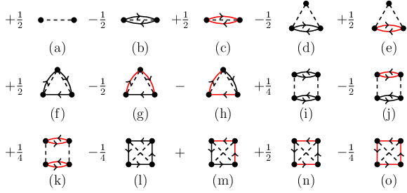
From the cluster expansion for the generating function we can construct the expansion for
| (5.18) |
Note, in particular, that the expansion of is irreducible. Diagrammatically, the corresponding expansion of the energy can be generated from the generating functional by generalizing the construction rules spelled out in Section 3.2 by
- 2.
To calculate the kinetic energy corrections replace any pair of exchange lines with one common point, , by a pair .

The last term, gives rise to the “energy numerator corrections” shown in (5.6). A discussion of the significance of these terms is found in Refs. 35 and 36. Basically, the formulation (5.6)-(5.9) amounts to a reformulation of the gap equation in terms of the -matrix as carried out, for example, in Ref. 113.
Cluster expansions for the energy numerator terms must be treated separately. These corrections consist of a series of products of diagonal matrix elements of the Hamiltonian, and off-diagonal matrix elements of the correlation operator. We classify the individual terms according to the number of common states contained in these two sets of matrix elements. The simplest, and dominating, energy numerator terms are those that have only one common state; in particular these are the only ones that survive in the weakly coupled limit discussed in Section 5.1. The derivation of these terms will be outlined in C. To express the construction rules, we need the following two generalized exchange lines
| (5.19) | |||||
| (5.20) |
where the are single particle energies generated from the ordinary CBF single particle energies by replacing all exchange lines by . The leading term in the is simply the kinetic energy .
The construction rule to obtain these diagrams from the generating functional is then:
5.3 FHNC and Euler equations
We formulate in this section the simplest version of the FHNC-EL equations, or FHNC//0 approximation. It is straightforward to formulate and implement the full FHNC equations [27]; in fact we have used the FHNC//1 approximation in our numerical applications. As above, the FHNC//0 form displays the physical content of the theory more clearly. Moreover, we shall show that corrections beyond the local correlation function are much more important than adding more complicated FHNC diagrams.
For further reference, we need the following quantities
| (5.21) | |||||
| (5.22) | |||||
| (5.23) | |||||
| (5.24) |
as well as their Fourier transforms , , , and . We begin with the expansion of the “dressed” correlation line . In FHNC//0, one keeps only the diagrams shown in Fig. 8 plus, of course, all longer chain diagrams and all parallel connections.

The FHNC//0 equations for a superfluid system are then identical to those for the normal system, except that the structure function of the normal system is replaced by the one of the BCS state,
| (5.25) |
where is the density operator. It has the form
| (5.26) |
From the definitions (5.26), (5.21), and 5.22) it is seen that the long-wavelength limit of is
| (5.27) |
Hence, for the superfluid system. The FHNC equations are, in this approximation, the same as Eqs. (3.20)-(3.22). Note, however, that we can in general not directly construct the pair distribution function from Eqs. (3.35), (3.36) if energy numerator terms beyond the kinetic energy are included.
The derivation of the Euler equation also is very similar to that for the normal system; the only change is that we must take the energy numerator terms into account. The then consists of three instead of two terms, the rule spelled out in Section 3.3 has to be augmented by
- 3.
Replace, in turn, each by . This may be thought of a correction to the second item .
5.4 Energy
Since the is, with replacement of the exchange lines by and described above, identical to that of the normal system, we only need to discuss the correction . We include in the energy numerator all those terms that have the same topology as those retained in the above energy expressions (3.34). There are the ones derived in B containing and as defined in Eqs. (5.24) and (5.23).
| (5.31) |
where is represented by the subset of diagrams containing only exchange lines. In our numerical calculations we found that the term is tiny, the term is henceforth omitted.
5.5 Uniform limit approximation
Eq. (5.29) has an interesting consequence: Note that the correction term does not contain correlation contributions. In other words it as also present even if the interaction is set to zero. The consequence of this is most easily seen in the “uniform limit approximation” [3] discussed in Section 3.5 which amounts to identifying in Eq. (5.29). The energy is, in this approximation [114]
| (5.32) |
The first terms in this expression is simply the (Hartree-Fock) energy expectation value with respect to the uncorrelated BCS state
| (5.33) |
and the remaining terms have been manipulated, using the Euler equation (5.29) in the uniform limit to eliminate .
Our result (5.32) demonstrates that the energy correction due to correlations is always negative. This result is not entirely surprising, it simply says that adding correlations will lower the energy expectation value. The more interesting statement is that the second term is negative even in a non-interacting system. The reason for this is that the BCS wave function (5.1), when projected to a fixed particle number, can be written in the form of an independent pair wave function [115]
| (5.34) |
where is the normalization integral, stands for antisymmetrization, and is a pair wave function given by the Fourier transform of . Thus, if we begin with an incorrect assumption about the Bogoliubov amplitudes (they are, of course, equal to normal state values , and for a non-interacting system) the Jastrow-Feenberg correlations try to compensate for that and lower the energy expectation value.
5.6 Euler equation for the Bogoliubov amplitudes
The study of the Euler equation has so far kept the Bogoliubov amplitudes fixed and only dealt with the optimization of pair correlations for such a fixed model state. In particular the analysis of the preceding section showed that the Jastrow correlations and the correlations implicit to the BCS wave function are not completely independent. It is clear that, in an independent step, the Bogoliubov amplitudes must also be optimized.
The derivation of the Euler-equation of the Bogoliubov amplitudes , follows closely the derivation of the conventional gap equation by minimization of the Hartree-Fock approximation [116]. One difference is that one has, in Hartree-Fock-Bogoliubov approximation, only one pair of and one pair of lines, see Eq. (5.33). The full variational energy expression in Eq. (5.11) can, on the other hand, have any number of these exchange lines. This means, in practice, that the effective pairing interaction and the single-particle energies depend implicitly on the , . The second difference is the appearance of the “energy numerator” terms .
As usual, we guarantee the normalization condition by setting
| (5.35) |
The minimization of the energy with respect to the can be done in both momentum and coordinate space. In coordinate space we have
| (5.36) |
or, in momentum space with
| (5.37) |
we have
| (5.38) |
Then, the optimization of with respect to results in
| (5.39) | |||
There are two contributions to the variational derivatives appearing in Eq. (5.39): One comes from and the other from the energy numerator terms . The variations of and with respect to or are best done diagrammatically by removing, in turn, from the expansion shown in Fig. 7 one exchange line and opening its external points.
- 1.
- 2.
The variation of with respect to the is constructed according to the same rules. It generally leads to a non-local pairing interaction of the general CBF form [23]. Since we keep, in the FHNC//0 version, only diagrams with or loops, we can write the result as
(5.41) where is diagrammatically obtained by (a) taking all diagrams in than contain only or loops, and (b) removing, in turn, each loop and opening its external points.
- 3.
We have restricted the discussion of the energy numerator terms to the simple approximation (5.31), omitting the second term. Then the variation with respect to yields two terms:
(5.42) The second term, which is proportional to , contributes a correction to the single particle spectrum whereas the first term gives a correction to the pairing matrix element. There is a third term, which we have not spelled out in Eq. (5.42), which originates from the implicit dependence of the single-particle energies on the . This term also contribute, if kept, to the shift of the single particle spectrum.
We can now write the minimization condition for the Bogoliubov amplitudes as
| (5.43) |
where
| (5.44) |
With that, we have brought the minimization condition for the Bogoliubov amplitudes in exactly the same form as the one for the weakly interacting system [116, 117], the remaining manipulations can therefore be skipped. The only change compared to the weakly coupled limit (5.9) is that all ingredients depend implicitly on the and the equation must be solved iteratively. Of course, in a more complete evaluation of the energy numerator terms as outlined in B, the kinetic energy terms in Eq. (5.44) are also replaced by the CBF single particle energies plus corrections from higher order diagrams. Also, note that the single particle energies and the pairing matrix elements depend implicitly on the Bogoliubov amplitudes. We also recover the weak pairing limit (5.6) by setting , , then .
5.7 Long wavelength analysis
The result (5.29) points to one of the major problems of local correlation functions and is, as such, one of the key messages of our paper. At the first glance, the result looks innocuous. Recall that we have discussed in Section 3.8 how Landau’s stability condition is a condition for existence of the parquet equations. In particular, within that limit, a negative value of is permitted.
If, on the other hand, the system is superfluid, we have , and therefore must be positive to have a solution. vanishes in the limit of a normal system whereas remains finite. Thus, if , the Euler equation ceases to have a solution even if the gap is infinitesimally small. We have shown this here only for the case of the FHNC//0 approximation, but it is also true in the general case that all FHNC diagrams, and possibly also higher-order correlation functions, are included since the Euler equation remains structurally the same, see Section 3.7. Our observation applies, of course, equally to “fixed-node” Monte Carlo calculations which may see this instability only in large stochastic fluctuations.
On a less drastic level, assume that . Eq. (5.29) then predicts the long-wavelength limit
which is obviously the wrong behavior since one should have . In other words, even if the interaction is repulsive, , Eq. (5.29) predicts the incorrect behavior of the static structure function at long wave lengths since the contribution of the free kinetic energy is missing.
This is evidently not a statement about the physics, but rather a statement on the approximations implicit to the wave function (5.2), specifically the collective approximation (4.5) for the Lindhard function. One can expect that the correct Lindhard function removes this spurious instability.
There have been several suggestions for a Lindhard function for a superfluid system [118, 18, 19, 21], the most frequently used form for is given below. In view of the need for the spin-spin response function in Section 6.1 we cite here both the spin and the density channels. In terms of the usual relationships of BCS theory,
| (5.45) |
| (5.46) |
where
| (5.47) | |||||
where the upper sign applies to the density channel, and the lower to the spin channel, respectively.
In the limit of a normal system, the coefficient become
| (5.48) |
as it should come out.
This superfluid Lindhard function is consistent with the as defined in Eq. (5.25).
| (5.49) |
We can now return to the frequency integration (4.2). All we need to show is that this expression exists, for small gaps, for . For that, it is sufficient to look at the limit of the static response function and the static Lindhard function.
For we get for the static Lindhard function
| (5.50) |
This is identical to the same limit of the Lindhard function of the normal system and leads to the correct stability condition.
Thus, the conclusion of our analysis is a more precise version of the statement made in Sections 3.8 and 4 about the validity of locally correlated wave functions for physical phenomena that involve mostly particles close to the Fermi surface. Previous work [28, 29] pointed out quantitative deficiencies; we have demonstrated here a much more profound problem, namely that there are indeed very serious qualitative difficulties in the sense that the minimization problem (2.8) has no solution. We stress again that this feature is not a consequence of the specific level of FHNC approximations. It is a general problem of the Jastrow-Feenberg form of the wave function. More elaborate versions of the FHNC summations and/or the inclusion of triplet correlations can change the numerical values but not the general features.
We conclude this section by recalling that the does not satisfy the -sumrule. Improved versions have been suggested [18, 21]. It would be very interesting to examine the wave function that corresponds to that work. Recall [121] that, to satisfy the -sumrule, the wave function must be an eigenfunction of the real-world Hamiltonian (2.1), which would be simply the Hamiltonian of a non-interacting Fermi system. Since that Hamiltonian commutes with the particle number operator, the wave function would also be, unlike the state (5.1), an eigenstate of the particle number operator.
6 Applicatios
Most of the calculations reported in this paper use the “weak coupling approximation” spelled out in Section 5.1 with the additional qualification that the “collective” Lindhard function (4.5) that was used throughout our earlier work was replaced by the exact Lindhard function in the rings and rungs. Only very few of the ground state properties changes visibly by including the superfluid Lindhard functions (5.46), we will mention that where appropriate. Only for the calculations of the gap function we have used also used the superfluid Lindhard function.
We have also used the simple RPA formulas (4.2) and (4.24) to sum the rings and rungs, for that it is appropriate to set . A more elaborate version of time-dependent Hartree-Fock is available [20] which should provide an interpretation of the correction ; we have not included this improvement because the corrections due to including the functions (5.46) are throughout very small, but computationally very time consuming.
6.1 Neutron Matter
Neutron matter is the first natural application of our method. It is of astrophysical interest because the magnitude of the superfluid gap is of critical importance for the cooling rate of neutron stars [122, 123, 124]. The system has been the subject of two extensive recent reviews [16, 17] which give a very complete account of the current literature. We can therefore restrict ourselves here to those aspects that are specific to the high-level many-body treatment of our paper.
From a quantitative point of view one should question the validity of the “weakly paired” approximation described in Section 5.1 because the gap is, at low densities, of the order of [125, 126, 36]. This concern is one of the reasons for developing the methods described in Section 5.
A few additions are necessary to deal with the dependence of the neutron-neutron interaction on the relative spin of the interacting particles. The Jastrow-Feenberg correlation function (2.3) does not contain spin-dependent correlations. It is, of course, straightforward to calculate the energy expectation value for an interaction of the type (6.1). Indeed, the spin-channel of the interaction gives an important correction to the energy; we have included it in Ref. 36. In the Euler equation, the spin-channel operator only contributes to the exchange terms discussed in Section 3.7; this correction is omitted in the FHNC//0 approximation.
Within CBF, it is also straightforward to include the simplest spin-correlations, either in low order perturbation theory [28], or by summing the CBF ring diagrams [24]. The latter provides an RPA-type energy correction from spin-correlations; the procedure then corresponds to an optimized “single operator chain” approximation [127].
6.1.1 Energetics
Let us now go through the relevant computations step-by-step. All intermediate results that are shown are for the Reid soft-core potential which we write in the operator basis [11]
| (6.1) |
We have carried out the identical calculations for the Argonne nucleon-nucleon interaction [128]. The results are sufficiently similar to those of the Reid potential; we will therefore display only the final results for that case.
The essential difference compared with what we have discussed in previous work [35, 129] is the operator form (6.1) of the interaction. Instead of a local , we have the spin–dependent interaction
| (6.2) |
where
| (6.3) |
in . Since the wave function (2.3) contains no spin correlations, there are no chain diagrams contributions to in the spin channel. In the CBF or parquet calculation, the appropriate interaction is then
| (6.4) |
where
| (6.5) |
We have commented above about the fact that the two ways to calculate , Eqs. (3.61) and (2.33) agree only in an exact theory. To assess the consistency between the two definitions, we have fitted, in the regime the equation of state by a function
| (6.6) |
and calculated from both the fit (2.33) and the long-wavelength limit (3.61). Here, and throughout the rest of this paper, we will set the effective mass ratio . Justification for this is derived from calculations of the self-energy as described in Sections 6.1.3, 6.2.3 and 6.3.1. Fig. 9 shows the situation for the low-density equation of state of neutron matter, interacting via the Reid potential.

We find in particular the FHNC//0 approximation for the particle–hole interaction leads to an incorrect positive value of . The FHNC-EL//1 approximation improves the agreements by including the exchange term in the particle-hole interaction, but it still disregards the chain-diagrams in the spin-channel who seem to be insignificant. These are included in the parquet calculations. The agreement between calculated in these two ways is, for low densities, evidently quite satisfactory.
6.1.2 Effective interactions
The energetics of neutron matter is relatively insensitive to the quality of the many-body wave function. We have already seen that this is not the case for the quasiparticle interaction. Similarly, one should expect visible corrections to the pairing interaction where medium polarization effects, especially due to spin fluctuations, are expected to have an impact on the superfluid gap [130, 131, 132, 133].
A very thorough examination of polarization effects has been performed by Schulze et al. [134]; our calculations go beyond that work in the sense that we determine the effective interactions by summing the parquet-diagrams, and take the superfluid particle-hole propagators. We have included the exchange terms that have been included in Ref. 134 in the localized form described in Section 3.7. Following the work of Ref. 134, we have also taken the dynamic interactions and at . The interactions derived from the FHNC approximation directly are, of course, energy independent.
A calculation for the superfluid phase that goes beyond the “weakly coupled” approximation requires the implementation of the full parquet-level theory because the Euler equations have, due to , no solution. Among others, we need the rather time-consuming computation of the superfluid Lindhard function which is an essential input for the theory. The fact that this is indeed necessary is documented in Fig. 10. There we show, for , the Lindhard function of the normal system, as well as the density- and the spin-channel of the Lindhard function of the superfluid system, Eqs. (5.46).
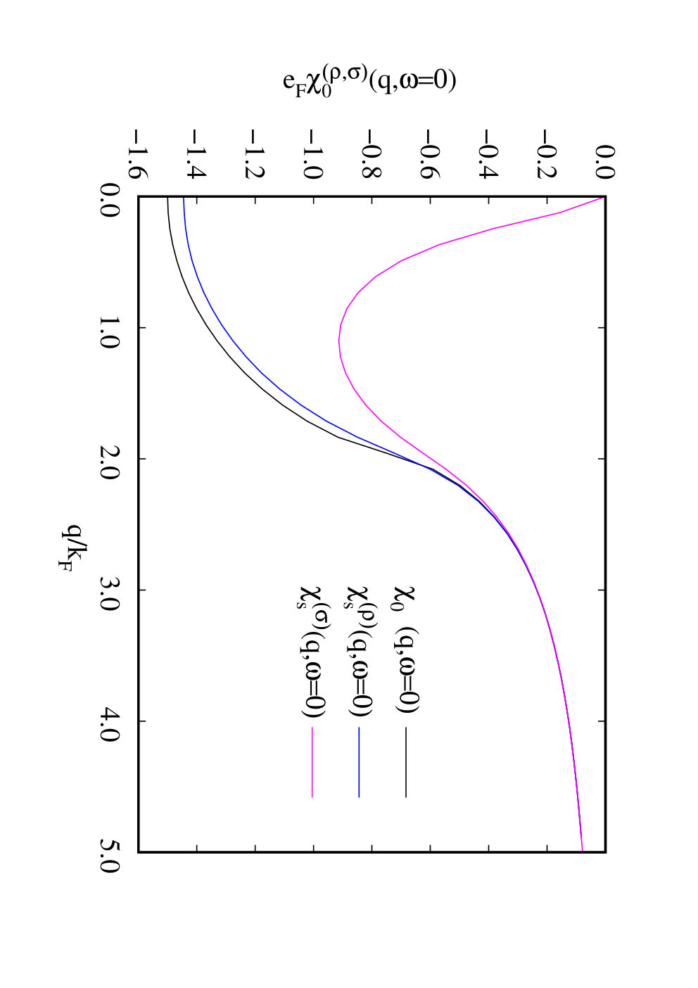
The discrepancy between the density and the spin-channel superfluid Lindhard functions is quite interesting and has, to our knowledge, not been noted in neutron matter calculations. It is caused by the fact that the superfluid Lindhard function in the spin-channel, Eq. (5.46) goes to zero as for all values of the gap. Of course, the regime where the spin-channel function deviates from the density-channel function becomes smaller with decreasing gap. The density-channel function is expectedly close to the one of the normal system even when the gap is relatively large.
This result has significant consequences for the effective interactions (6.5). These interactions are shown in figures 11 and 12


The conclusion to be drawn from Fig. 11 is that the use of the dynamic effective interaction in the density channel potential at makes the interaction somewhat less attractive, but there is practically no difference between using the normal system Lindhard function or the one for the superfluid one. The situation is quite different in the spin-channel: Using the superfluid Lindhard function changes the effective interaction in that channel significantly, note that the gap at the density considered here is only about 20 percent of the Fermi energy, see Fig. 15 below. This is to a large extent due to the fact that superfluid goes to zero at zero momentum transfer. The particle-hole interaction and the paring interaction are therefore identical in that limit. This is not the case if one uses the normal system Lindhard function to calculate .
In the pairing matrix elements, we must couple the interactions (6.5) into the singlet and triplet channel:
| (6.7) | |||||
| (6.8) |
The most relevant quantity for our purposes is the singlet pairing interaction which is shown in Fig. 12. Similar to the spin-channel, using the superfluid Lindhard function changes the interaction visibly, in particular for long wavelengths which is the important regime for pairing phenomena. Interestingly, the choice of the superfluid Lindhard function suppresses the correction from spin-fluctuations; the -wave interaction is closer to the one where the spin-channel is omitted altogether than to the one where the spin part is taken from the normal system.

6.1.3 Self energy
We have spelled out in Eqs. (3.73), (3.74) and (3.75) working formulas for the single particle spectrum based on a local correlation operator. In Section 4.4 we have then made the connection to the G0W approximation and have shown how these two procedures are related. The situation is similar to the one for other quantities: FHNC offers a much more extensive summation of diagrams. Note, for example, that the denominator can be related to high-order exchange diagrams but has no equivalence in the G(0)W approximation. The price for that is that the evaluation of these diagrams is less accurate. We shall address these issues now.
We are examining the self-energy here for a number of reasons. One is to justify our choice of keeping only the kinetic energy in and , Eqs. (5.19) and (5.20), defining . The second reason is to justify the use of a free spectrum in the gap equation (5.9). We have studiend the sensitivity of the superfluid gap agaist changes of the effecive mass in Ref. 36.
The self energy (4.30) is most conveniently evaluated by Wick rotation in the complex - plane. That way, the RPA sum for the self-energy is decomposed into two terms, a smooth “background–” or “line–term”, which consists of the frequency integral along the imaginary axis, and a second, “pole term” from the residue of the single-particle Green’s function, i.e.
| (6.9) |
with
| (6.10) |
and
| (6.11) | |||||
Since the effective mass can have an visible effect on pairing properties, we have calculated the ratio
| (6.12) |
from the on-shell self-energy for both the Reid and the Argonne potential; results are shown in Fig. 13. The effective masses are all close to 1, suggesting that the single particle spectrum of non-interacting fermions is an adequate approximation in this particular system. It also justifies the on-shell approximation. While the effective mass ratio per-se is close to 1, we see that the corrections from going beyond local correlations are substantial on that scale.

It is also of interest to look at the individual contributions to the self-energy as a function of wave number. We show these in Fig. 14.

The FHNC expression for the static field (3.74) and the “Fock” differ only by the interaction entering the expression: Whereas tilde is defined in terms of the full static interaction , the static field contains only the particle-hole irreducible interaction . Evidently these two terms are numerically rather similar. The remaining two terms, and , sum to practically a constant, hence the real part of the spectrum is, at this density, indeed rather similar to the FHNC approximation. We also see that there is, in neutron matter, no visible enhancement of the effective mass around the Fermi surface as observed in nuclear matter [100]. This is consistent with the fact that imaginary part of the self-energy is rather small.
These results essentially confirm that our choice of is justified.
6.1.4 BCS pairing
We have generally solved the full gap equation (5.9), using the eigenvalue solver with an adaptive mesh described in Ref. 35. Results will be reported for the value of the gap function at the Fermi surface, .
Several approximate formulas for the superfluid gap at the Fermi surface are available: At very low densities, the gap can be expressed in terms of the vacuum scattering length [113] as
| (6.13) |
The exponential is universal in the sense that it depends only on the product , but not on details of the interaction. The pre-factor is modified by polarization corrections [135] which are also universal, and by many-body and finite-range corrections some of which are non-universal [35].
Eq. (6.13) gives, apart from very low densities, quite poor predictions. More useful is the estimate
| (6.14) |
where
| (6.15) |
is the -wave matrix element of the pairing interaction at the Fermi surface. Eq. (6.14) shows clearly the influence of the effective mass correction; we have studied this in Ref. 36. Since the effective mass is always close to the bare mass, see Fig. 13, we have throughout this paper used .
Our results for the superfluid gap are shown in Figs. 15, they basically reflect our findings on the pairing interaction. Including exchanges does not change the gap significantly; the most significant change comes from using the dynamic interaction , Eq. (6.7). Using the superfluid Lindhard function moves the result a little up but is somewhat unexpectedly not very significant, despite the suppression of the long-wavelength components in as demonstrated in Fig. 10. The approximation (6.14) underestimates by about a factor of 2. We also show the results obtained from the estimate (6.13) using the experimental -wave scattering length fm [136].


We have, in the neutron matter calculations, only solved the parquet- equation in the density channel because our primary interest is the pairing interaction; in the spin–channel we have only kept the polarization diagrams. One can extend the calculation to include spin- and tensor- operators [137] in the full parquet summation.
6.2 The Lennard-Jones liquid
Fermi fluids interacting via a family of Lennard-Jones (LJ) interactions
| (6.16) |
have been studied extensively in Refs. 72 and 35. The system is interesting from the viewpoint of many-body theory since the equation of state can have two spinodal points where the hydrodynamic speed of sound (2.33) vanishes. For the sake of discussion, we show in Fig. 16 a schematic equation of state for a typical self-bound Fermi liquid.

The dominant energy contribution at very low densities is the Pauli repulsion, . As the density increases, interaction terms, which grow as , begin to dominate and bend, if the interaction is sufficiently attractive, the equation of state downwards. This leads to a local maximum. If that is the case, the equation of state also has a local minimum at some finite density before the short-ranged repulsion begins to dominate. Hence, there must be two spinodal points. The Lennard-Jones liquid shows, for sufficiently large values of the interaction strength , both of these points. In contrast to that, an attractive square-well potential or the attractive Pöschl-Teller interaction studied in Ref. 125 and in Section 6.3, has only the lower spinodal point. These systems collapse, due to the absence of a short-ranged repulsion, when the density is increased to a level where the interactions begin to dominate over the Pauli pressure. Neutron matter is not self-bound and does not show spinodal points.
6.2.1 Energetics and stability
We discuss in this section our results for the above family of Lennard-Jones 6-12 interactions. The strength or, better, the dimensionless strength parameter of the interaction can be adjusted such that the interaction has the desired vacuum scattering length; a bound state and a corresponding singularity of the vacuum scattering length appears at . Fig. 17 shows the scattering length for both the Lennard-Jones and the Pöschl-Teller (PT) interaction discussed in the next section as a function of the potential well depth. We also show, for comparison, the scattering length for the attractive square-well interaction discussed in Ref. 35.
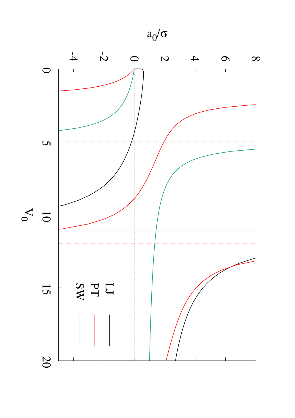
Before we discuss our findings, we comment on the expected accuracy of our results. This was examined in Ref. 72 where we found that the FHNC//0 approximation is accurate within a percent at low densities up to approximately 25 percent of the saturation density. This corresponds to a Fermi wave number of or a density . This is the regime of interest here. Around saturation, the FHNC//0 approximation still displaus the correct physics, but leads to an equation of state that is somewhat too soft. The numerical values in that regime should be therefore be considered only qualitative. These observations apply, of course, predominantly to the energy which is relatively insensitive to the quality of the wave function. The stability range is indeed affected, even at low densities, by including the exchange diagrams discussed in Section 3.7.
We have studied here a density regime of , and interactions strengths . In Ref. 35 we went to the much smaller values of . A proper treatment of many-body effects requires that the simulation box is much larger than . On the other hand, the core region must be properly resolved, hence decreasing the minimum value of by an order of magnitude increases the necessary number of mesh points on an equidistant mesh (as required by the fast Fourier transformation algorithm) by an order of magnitude. In Ref. 35 we have worked with mesh points; since the implementation of Eq. (4.2) required by the parquet-level calculations implies an energy integration for each mesh point, we have reduced in this work the number of mesh points to . This limits the minimum density to the above value. Since the lower spinodal points move, with interaction strength, to lower densities, this constraint also limits us to interaction strengths .
The equation of state of for a sequence of interaction strengths is shown in Fig. 18. Results for stronger interactions are not visible in the figure and have been omitted. The figure shows clearly the gap in the equation of state between the two spinodal points which appears when the interaction is sufficiently strong, .

The most interesting result of Ref. 35 is that the FHNC-EL equations diverge, at low density and as a function of density, well before the lower spinodal point is reached. To examine this effect more closely, we have included the two improvements discussed in Sections 3.7 and 4.1. As mentioned above, the inclusion of the exchange diagrams shown in Fig. 5 can indeed change the long-wavelength limit of by a factor of and, hence, can in principle increase the stability regime significantly.
The second correction is due to the transition from the variational wave function to parquet diagrams. A summary of our results for the Fermi liquid parameter is, for the sequence of interaction strengths used in Fig. 18, shown in Figs. 19.

The most visible (and expected) quantitative correction is caused, at low densities, by the inclusion of exchange diagrams. Fig. 20 shows, for four selected densities close to and above the density where spinodal points exist, the as calculated on the FHNC//0 approximation and the parquet//1 approximation. A number of observations apply: First we notice that the results with and without including exchange diagrams differ, in particular in the low density regime, by roughly a factor of 2. This is consistent with the argument of Section 3.7 that the leading term in the density expansion is reduced by exchange diagrams. The factor of is visible in the slope of at as a function of . (The argument does not apply to the nuclear case since the interaction in the exchange channel is different from the one in the direct channel, see Fig. 9 and Eq. (6.3).) The second, and much more interesting, observation is that the density where the FHNC-EL equations diverge is almost independent of the inclusion of exchange diagrams.
The FHNC and the parquet results are, at the same level of implementation, almost indistinguishable. The inclusion of the correct particle-hole propagator only limits the regime of existence of solutions to the regime but has otherwise little effect. Evidently, the existence of the spinodal points does not change qualitatively with the parquet theory developed in Section 4, however, the location of the divergence changes somewhat.

To assess the accuracy of our predictions we have again carried out the consistency test between the between obtained from the equation of state, (2.33) and from the long-wavelength limit (3.61), . At the strongest couplings, , the coefficient of the term cannot be determined reliably, we have therefore kept only the linear in Eq. (6.6). A comparison of the two procedures is shown in Fig. 21; evidently the agreement is in the regime of interest not quite as good as in the nuclear case, this is because the density dependence of the correlations cannot be ignored.

As in previous work [35] we found that it is impossible to find solutions of the FHNC-EL or parquet equations close to the lower spinodal point. The fact that the equations of state all come to an endpoint has been identified in Ref. 35 as due to a divergence of the in-medium scattering length which is, in the local approximation used here
| (6.17) |
This divergence is the reason that the Landau stability limit could not be reached. The same situation occurs, expectedly, in the present case, see Fig. 22. One might have argued that the divergence found previously is indeed just the spinodal instability and one could not get closer due to some numerical problem. The comparison of the FHNC//0 and the parquet//1 results shown in Fig. 20 shows that the divergence found here is indeed unrelated to the Fermi liquid parameter: It appears at practically the same density, although the differ by a factor of 2.

Thus, our conclusions on this topic have not changed, moreover, we have eliminated the most relevant concern about our previous work, namely that the Landau parameter has not been calculated accurately enough.
6.2.2 Effective interactions and correlations: A configuration space view
We have throughout the preceding sections emphasized the momentum space properties on effective interactions, in particular the connection between the long wavelength limits, Fermi liquid parameters, the in-medium scattering length, and the pairing interaction. Of course, the structure of correlations is mostly determined by the short–ranged properties of the interactions. Given the knowledge about the bare interactions, the short–ranged structure of the correlation functions is given by the Bethe–Goldstone equation which is, in its essence, a zero-energy Schrödinger equation where the short-ranged structure of the pair wave function is modified by the Pauli principle [88, 87, 74].
The relationship between the pair correlation function , the “dressed” correlation function and the pair distribution function has been discussed in many places, we therefore focus here on the low-density expansions (3.35), (3.36). Fig. 23 shows, at the relatively low density of a sequence of pair correlation and distribution functions. The “dressed” correlation function describes the dynamic correlations and is determined by the bare interaction. The pair distribution function contains, in addition, statistical correction manifested predominantly in the factor in Eq. (3.35), but also in the corrections and , cf. Eq. (3.36). Fig. 23 also shows the simple approximation for the pair distribution function. Evidently, the correction from chain diagrams, is not negligible; we assert, however, that the contribution from the exchange parts are invisible on the scale of the plot.

The dynamic correlations determine the effective interactions via Eqs. (3.27) and (3.28) and . Aldrich and Pines [83, 84] give a physically intuitive description of the effects contributing to which is called “pseudopotential” in that work:
- 1.
At short distances, the interaction is screened by short-ranged correlations;
- 2.
The fact that the wave function is bent at short distances – downwards for repulsive interactions, upwards for the attractive interactions as in the attractive square well potential and the Pöschl-Teller potential – has a price in kinetic energy;
- 3.
Finally, the presence of other particles should lead to an enhancement of the interaction in the attractive regime.
Eqs. (3.27) and (3.28) give a quantitative meaning to these effects: The short-ranged screening (1) is described by the factor , the cost in kinetic energy is described by the term , and many-body effects are described by the last term . Fig. 24 shows these three parts of the particle-hole interaction at and an interaction strength . We had to scale the induced interaction term by a factor of 100 to make it visible at the scale of the plot. This does not mean that this term is negligible; it guarantees that the dynamic correlation function falls off as as . cf. Eq. (3.39).

Fig. 25 shows, finally, the dependence of at on the interaction strength for the sequence . We have not included the exchange correction, it satisfies to an extremely good accuracy our estimate .

6.2.3 Effective mass
The Lennard-Jones interaction may be thought of a model for the interaction between helium atoms. More modern interactions [138, 139, 140] are perhaps more accurate; but the Lennard-Jones model reflects the correct physics of 3He. In our parametrization that uses the core size as unit of length, and as unit for the energy, 3He is characterized by and the equilibrium density has a Fermi momentum , in other words the equilibrium properties of 3He are beyond the regime where out approximations are reliable. See Ref. 72 for a discussion and full FHNC-EL calculations.
Liquid 3He is known to undergo below 3 mK superfluid phase transitions [141, 142] to two different phases of -wave superfluidity. At the experimental saturation density of 3He, the soft spin-fluctuation mode is very important and is the essential mechanism for the strong effective mass enhancement around the Fermi momentum [93, 103, 104, 105]. If both backflow and spin-fluctuations are omitted, one ends up with an effectiv mass less than 1 [143]. We are in this work interested in low-density systems and potential -wave pairing. We will see below that -wave superfluidity can occur only at very low density; in particular below the lower spinodal point which is around for , see Fig. 19. Therefore, we expect that the much simpler G0W approximation spelled out in Eqs. (4.30), (4.31) is adequate.
Fig. 26 shows the effective mass obtained as described above way for a sequence of interaction strengths . Throughout, the effective mass never differs from the bare mass by more than 10 percent. Interestingly, we find for the most repulsive interactions a slight reduction of the effective mass ratio which turns into an enhancement around and then above again into a reduction.
The explanation for that is that the value of the effective mass ratio is an effect of both Fermi statistics and hydrodynamic backflow. Fermi statistics has mostly (but not always) the effect of reducing the effective mass, this is a well-known effect in nuclei [100] but also comes out for 3He in the naïve formulation (3.73) [127]. Hydrodynamic backflow [144] increases the effective mass. That effect is included in the G0W approximation which includes hydrodynamic backflow; see Ref. 27 how Feynman’s backflow operator comes out already in second order CBF perturbation theory. In this work, we have not included spin fluctuations, hence the results shown are only due to Fermi statistics and backflow. Apparently, backflow effects become stronger with increasing attractiveness of the interaction. This makes sense because more particles are relatively close to each other; see Fig. 23 how the nearest neighbor peak increases. For that to be effective, of course the density must be high enough.

6.2.4 BCS pairing
Let us now turn to the calculation of the superfluid gap. By construction, our pairing interaction contains polarization corrections, see the discussion of the connection between parquet theory and FHNC-EL in Section 4, cf. Eqs. (4.23). These polarization corrections are important modifications of the pairing interaction and can lead to significant changes of the superfluid gap, see, for example, Refs. 131, 132, 133, 134
The details of the choice of interactions (6.5), i.e. if exchange diagrams are included and whether we take the collective Lindhard function or the energy dependent one, define different implementations of the pairing interaction in FHNC or parquet diagram theory. Using local correlations means that the Lindhard function is replaced by the collective Lindhard function defined in Eq. (4.5), and taken at the average frequency , Eq. (4.27). In FHNC//0 approximation, this leads to the expression (4.26) which was used in previous work [35, 36]. The equivalence between FHNC and parquet-diagrams permits us, however, to be more flexible. Since the pairing gap is expected to be relatively small one is led, in the parquet version the theory, to take the pairing interaction at zero frequency [134].
Our results are shown in Fig. 27. Indeed, both modifications, exchange diagrams and using the sero-energy Lindhard function for the particle-hole propagator can cause a change of up to a factor of two in the superfluid gap; the effect is about half due to exchange diagrams, and half due the propagator correction. The right pane of Fig. 27 shows a comparison of the solution of the full gap equation with the two approximations (6.13) and (6.14).

A somewhat surprising result is that fully self-consistent theory where all particle-hole propagators (5.46) are taken for the superfluid system causes, despite the smallness of the gap, a visible effect in the stability regime as indicated by the end of the respective lines. Apparenty, being close to an instability, makes every quantity sensitive to small details.
In the model we have considered here it seems impossible to get close to the “BCS-BEC” crossover regime. The reason for lies both in physics and in formalism: From Fig. 19 it is clear that one is, whenever the superfluid gap is sizable, close to the lower spinodal point, even if one cannot reach it. For systems like the one studied here, and, even more, for the attractive Pöschl-Teller interaction studied in the next section, one has two competing effects: To get a stronger gap, one needs a more attractive interaction. Such an attractive interaction has, on the other hand, the effect that the Pauli-pressure is more easily overwhelmed by the interaction and, hence, the spinodal point moved to lower densities.
The formal reason is also quite plausible: The implementation of FHNC-EL or parquet theory involves two sets of diagrams, rings and ladders. A third set, the “cyclic chain” diagrams that would indicate a divergence of the single particle propagator which might be present in spin-polatrized 3He [145] has not been considered here. A divergence of the ring-diagrams is related to the existence of spinodal points or, more generally, to Landau’s stability conditions . What we find, however, is a divergence in ladder equation (3.33). It is harder to associate that with a specific quantity because the induced interaction always tries to adjust itself such that the has zero scattering length and that, therefore, Eq. (3.33) has a solution with the property as , see Eq. (3.39). But it is easy to envision that the potential becomes attractive enough such that the equation develops a bound state. This has the consequence that falls off exponentially as . Then the basic assumptions of the equations of the theory are violated and it is no surprise that they have no solutions. This is apparently what happens here, where the effect is caused by the attractiveness of the induced interaction which describes predomilantly phonon exchange. Hence, we have concluded in Ref. [35] that the divergce is due to a dimerization caused by phonon exchange, in other words it is a genuine many-body effect.
This is an interesting statement per-se: Note that in a weakly interacting system, the gap equation can describe the transition between a “BCS” state where the Cooper pairs are weakly coupled, to a “BEC” phase where the pairs are strongly bound [146]. The gap equation is a proper subset of our diagram summation; but we find a divergence of a set of diagrams that are not included in weakly interacting systems described by the gap equation alone. The issue deserves further investigation.
6.3 Pöschl-Teller interaction
The purely attractive Pöschl-Teller (PT) interaction [147]
| (6.18) |
is characterized by the strength and the range . For this interaction, the scattering length can be calculated analytically [148].
| (6.19) |
where is Euler‘s constant. The interaction is somewhat more convenient to use in Monte Carlo calculations than the square-well interaction [149]; it has been used in Ref. 125 to study pairing in the unitary limit. We have recently examined the ground state and pairing properties of the Pöschl-Teller gas [129]; in this work we have improved these calculations by applying the improvements outlined above. Since many techical details have been discussed in the preceding sections, we can restrict ourselves to display just the new aspects of our calculations.
6.3.1 Energetics and stability
Since the Pöschl-Teller interaction does not have a repulsive core, there is no self-bound, high-density phase. The low density properties are basically determined by the balance between the Pauli repulsion and the attractive interparticle attraction. Our findings for the PT interaction are sufficiently similar to those of the LJ interaction sich that we can be very brief..
Fig. 28 shows the equation of state, normalized to the kinetic energy of the free Fermi gas. In the limit of low densities, the equation of state should be give by the Huang-Yang expansion (3.60), we have studied this in Ref. 35 for the Lennard-Jones and the attractive square-well model and found that the term proportional to is already overshadowed by non-universal many-body effects. We compare therefore only the linear term in the expansion (3.60) and restrict, of course, the expansion to small values of . Similar to our previous work we find that the expansion (3.60) is reasonably accurate for , see Fig. 29.


Fig. 30 shows the Fermi liquid parameter as obtained from Eq. (3.61) for the same sequence of interaction strengths as used in Fig. 28 as a function of the density. In general, there is little qualitative change; the stability regime is changed visibly by including exchanges, but the result that there is no way to get close to Landau instability regime is not changed; in fact, the most advanced calculation leads, similar to the Lennard-Jones model, to a much smaller value of where the divergence occurs. Due to this instability we have not been able to reach the rather large values of reported in Ref. 125 before the system became unstable. We have again checked the consistency between Eqs. (2.33) and (3.61) with the procedure outlined in the previous section. We found that the numerical values are practically identical for weak couplings when exchange diagrams are included.

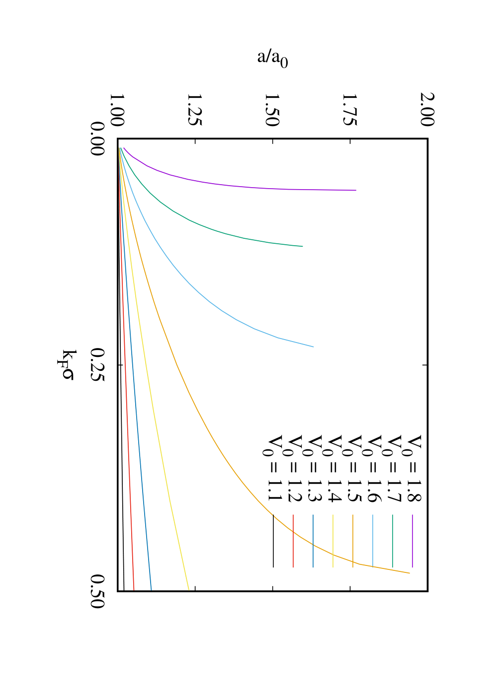
For completeness, we show in Fig. 31 the effective mass ratio for the above sequence of coupling strengths. As in our previous calculations, these ratios are close to 1 which is certainly a consequence of the low density of the system.

6.3.2 BCS pairing
Fig. 32 shows the calculated energy gap in FHNC//0, parquet//1 and fully self–consistent approximation. Evidently, inclusion of the energy-dependent effective interaction can change the value of the gap visibly. This is, of course, not a statement on the specific FHNC approximation, but more generally on the quality of the locally correlated (or “fixed-node”) wave function. The fully self-consistent calculation brings us here back into the vicinity of FHNC//0, we hasten to point out that this observation is circumstantial and should not be generalized.

In conclusion, we note again that the most important change duu to going beyond the “weak coupling” approximation (5.5) is that the stability regime is further reduced.
7 Discussion
We have formulated in this paper the variational and parquet approach for strongly interacting, both normal and superfluid, systems. We have then studied the Euler equation for the local correlations in a version that exhibits all the exact properties of variational and parquet-diagram theories but does not require the formulation of the full FHNC theory. We have derived the interesting, yet disturbing, result that the Euler equation for locally correlated wave functions of the form (2.3) has, for a superfluid system, no physically meaningful solution for net attractive interactions , and displays pathological features even for repulsive interactions.
The problem is caused by the very form of the Jastrow-Feenberg wave function. The plausible way solve this problem is by comparison with parquet-diagrams. This has been carried out in Section 4, and that formulation can be naturally carried over to the superfluid system. That has the effect that the “collective approximation” for , Eq. (5.29) is replaced by the RPA expression (4.2). The formulation of Coupled Cluster theory with correlated wave functions [31] would perhaps be another way to carry this through, but, on the other hand, our result is sufficiently convincing.
We have then carried out numerical calculations for different model systems of physical interest: neutron matter and model systems interacting via a family of Lennard-Jones and Pöschl-Teller interactions. With the recent interest in pairing in cold gases and the BEC-BCS crossover, it has become fashionable to stress the similarity between cold gases and neutron matter. In fact, the neutron scattering length fm [136] which is much larger than the range of the interaction. We found in this work that these systems are actually rather different. Whereas there was no problem calculating the properties of neutron matter at all densities, the parquet-equations showed inevitable divergences for both the Pöschl-Teller and the Lennard-Jones interactions at scattering lengths of the order of . The divergence is driven by the approaching of a “soft mode” at the spinodal points(s) , but not caused by it. Spinodal points appear in both the Pöschl-Teller and the Lennard-Jones interactions, see Figs. 19 and 30, but neutron matter is far from such an instability, see Fig. 9. The cause of the instability rather seems to be a divergence in the ladder equation.
Monte Carlo simulations for a square-well interaction seem to indicate that the equation of state comes close, but do not reach, a spinodal decomposition before the BEC-BCS crossover is reached [150]; the data of Refs. 151, 125 are too sparse to make a conclusive statement.
Two points should, of course, be emphasized: One is that the “fixed-node” wave function displays the spurious instability discussed extensively above. Simulations based on such a wave function will at their best converge to the infimum of the energy that can be reached by wave functions of the type (5.2). Another problem arises since an exact simulation should converge towards the exact ground state, which could also be a droplet or a film covering the walls of the simulation box. However, we are interested here in the features of the uniform, but metastable state that can be present close to the spinodal point. We believe that this problem deserves a very careful examination.
The most serious problem in the application to nuclear systems is that there is evidence that parquet-class of diagrams is not sufficient for reliable calculations [152]. Unfortunately, this is insufficient when the core or the interaction is very different in the spin-singlet and the spin-triplet channel. In that case, the so-called “twisted chain” diagrams can be very important. We must keep this problem in mind but leave it for future work. In the language parquet theory, the “rungs” cannot be considered to be local interactions, but all time-orderings must be kept. In the language of the Jastrow-Feenberg method, the so-called commutator diagrams are important. The effect can be very dramatic. We will examine this in future work on neutron matter.
Appendix A Cluster expansions for the generating function. Diagonal terms
We show in the following series of appendices some details of the calculation of the generating functions given in Eqs. (5.12) and (5.13). First, we calculate the cluster expansion of the : Define
| (A.1) |
where is the sum of all cluster contribution containing points and correlation lines . The individual terms of the cluster expansion are identical to the expansion of the normal ground state if we re-interpret the exchange line as
Next, we formulate the resulting matrix elements as matrix elements of a diagonal second quantized operator,
| (A.2) |
where
| (A.3) |
where stands for some permutation of the quantum numbers , and is a combination of correlation lines connecting points. The leading order terms are
| (A.4) | ||||
| (A.5) |
Finally, we calculate the expectation value of these operators with respect to by the usual contraction technique [153, 110]
| (A.6) | ||||
| (A.7) | ||||
| (A.8) | ||||
| (A.9) |
where , refers the states with opposite momentum and spin of the states , , respectively, and () when the spin of is up (down).
| (A.10) |
and
| (A.11) |
The diagrammatic representation of the two-body contribution (A.10) is shown in the diagrams (a) and (b) in Fig. 6 whereas corresponds to twice diagram (f) and diagram (d) of that figure.
We have to address a somewhat subtle issue connected with the appearance of “equivalent” diagrams which have a different topological structure, but the same value. Diagrams (d) and (e) of Fig. 2 are the simplest example. In the normal system it is easily seen that these diagrams have the same value because the exchange function satisfies the “convolution property:
| (A.12) |
In contrast, as pointed already out in Ref. 110, the convolution property does not hold for the exchange lines. Superficially one might therefore expect to get two different expressions for diagrams 4 and 5. An immediate consequence would also be that the expansion becomes point-reducible [110]. We therefore examine the issue here carefully.
We go back to the expansion (A.1), represented diagrammatically in Fig. 2. Diagram (e) can be written as
| (A.13) |
The last equation holds because also satisfies the convolution property (A.12). The latter representation has then to be written in the second quantized form (A.3) which gives the correct weight factor of diagram (f) in Fig. 6.
The reason why these diagrams must be collected before calculating the expectation value with respect to the is that we have two disconnected correlation lines in leads additional momentum conservation:
which would give a zero contribution to the second-quantized form. A very similar consideration was necessary for the calculation of the CBF single particle energies (3.69), see Ref. 23.
Appendix B Cluster expansions for the generating function. Off-diagonal terms
To derive cluster expansions for the generating function we can use again the power-series method explained in Section 3.2 and define the normalization of as
| (B.1) | |||||
where is given by
| (B.2) |
with
| (B.3) |
see Eq. 3.67. We now use the power-series method [71] described in Section 3.2 to obtain a cluster expansion
| (B.4) |
We can then write a term with correlation lines as
| (B.5) |
where the are -body clusters with lines. We then write these as off-diagonal matrix elements of second quantized operators
| (B.6) | |||||
A few leading order terms, where the states and differ by exactly two states, are
In this formulation, we can calculate the expectation values of these operators with respect to . The diagrams contributing to containing one or two correlation lines are shown in Fig. 33.
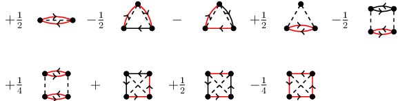
As a matter of course we have to pay again attention to the appearance of equivalent diagrams which must be combined before the BCS expectation value is calculated. Since the operations are identical to those outlined for the diagonal components in A, we skip this step.
Appendix C Cluster expansions for the energy numerator terms
In this appendix, we show details of the calculation of the energy numerator corrections defined in Eq. (5.11). We begin with the definition
| (C.1) |
We can again use the power-series method to generate a cluster-expansion for . Unlike above, we expand the diagonal matrix elements and the off-diagonal matrix elements individually. Analogously to A, we can write the diagonal matrix elements of the Hamiltonian in terms of a sum of diagonal, second-quantized -body operators
| (C.2) |
Similarly, we write the matrix elements in the form (B.6). Then, each single contribution to the sum in the numerator of Eq. (C.1) has the form
| (C.3) | |||||
The expectation values of the creation and destruction operators with respect to are then done with the usual contraction technique [153]. Unlike above, we now have two groups of creation and annihilation operators: The group belonging to the diagonal matrix elements, and the group belonging to the . We now classify the expansion in terms of the number of contractions between the two groups. The term where only operators within each group are contracted with each other cancels the second term in the above equation.
Hence, the simplest contribution is the set of diagrams where one pair of creation/destruction operators of the set is contracted with one pair of the group . All other contractions of operators of the set are done just as for the and the resulting . It is clear that the resulting quantity can depend only on the quantum number of the state that has been contracted with the group . Hence, we can think of these contributions as a one-body operator
| (C.4) |
where
| (C.5) |
and denotes the Fourier transform defined as (2.10), and is the momentum carried by the common state .
The leading term in is kinetic energy , higher other correction terms to are shown in Fig. 34. They reduce to the CBF single-particle spectrum in the normal system if one replace by .

We can now rewrite as
| (C.6) |
where
| (C.7) |
and can again be expanded in a cluster expansion as in B:
| (C.8) |
A few leading order terms in are given by
| (C.9) | ||||
| (C.10) |
Thus, we can define
| (C.11) |
We give details of the calculation here only for two typical terms: The two-body term is
The rest of the calculation is performed by the usual contraction technique which leads to
| (C.13) |
This leads to diagrams (a), (b), and (c) shown in Fig. 35, where the black and red double-arrow respectively stand for a kinetic exchange lines,
| (C.14) |

A new structure comes it at the next order, :
We look only at the first term in in Eq. (C.10) which is evaluated as
| (C.16) | |||||
The first two terms are represented by diagrams (d), (e), and (f) in Fig. 35 and the last term is represented by diagram (g) in Fig. 35.

The diagrams we obtained in Fig. 35 can be further simplified by introducing the modified exchange lines and defined in Eqs. (5.20) and (5.19). We represent and by black and red double arrowed lines as shown in Fig. 36. For instance, the diagrams (a), (b), and (c) in Fig. 35 can be combined as the first diagram shown in Fig. 37.

To summarize, we can write the energy numerator terms containing one contraction the and the groups in the closed form
| (C.17) |
The two variational derivatives with respect to and can be done with the same diagrammatic techniques as the ones used in 23 for the calculation of the single-particle energies. It leads to the co-called “cyclic chain” diagrams already mentioned in Section 3.2. We have in the further analysis obtained only the leading terms which have been spelled out in Eq. (5.31).
The procedure can be easily extended for the case of two, three, …contractions between the and the groups. Instead of a diagonal one-body operator , one obtains two, three, …operators in Eq. (5.31). We will not pursue this further because we did not include these terms in our calculations, and they disappear in the weakly coupled limit whereas the terms examined here lead to the energy numerator terms in Eq. (5.6).
The same consideration can be used to calculate the correction to the superfluid density due to correlations, note that we have pointed out in connection with Eq. 5.15 that the quantity defined there is not the same as the density
| (C.18) |
where is the density operator. We can write
| (C.19) |
where . Since the particle number operator commutes with the correlation operator , the second term in Eq. (C.19) has exactly the same structure as Eq. (C.1). We can then go through the further steps of the calculation, with the simplification that the number operator is a constant one-body operator. The result is therefore immediately obtained by replacing the one-body operator by the number operator. Since this is the same as taking just the constant term , we can immediately conclude that
| (C.20) |
with
| (C.21) | |||||
| (C.22) |
Appendix D Calculation of exchange diagrams
A working formula for these exchange diagrams is [154]
| (D.1) |
is conveniently calculated by an expansion in spherical harmonics:
| (D.2) |
which gives
| (D.3) |
with
| (D.4) |
Here
| (D.5) |
With that, we get
| (D.6) | |||||
and
| (D.7) | |||||
Acknowledgment
This work was supported, in part, by the College of Arts and Sciences, University at Buffalo SUNY, and the Austrian Science Fund project I602 (to EK). We would like to thank Grigori Astrakharchik, Jordi Boronat, John Clark and Peter Schuck for useful discussions on the subject of this paper.
References
- [1] A. L. Fetter, J. D. Walecka, Quantum Theory of Many-Particle Systems, McGraw-Hill, New York, 1971.
- [2] H. Kümmel, K. H. Lührmann, J. G. Zabolitzky, Many-fermion theory in expS- (or coupled cluster) form, Physics Reports 36 (1978) 1–63.
- [3] E. Feenberg, Theory of Quantum Fluids, Academic, New York, 1969.
- [4] A. D. Jackson, A. Lande, R. A. Smith, Variational and perturbation theories made planar, Physics Reports 86 (2) (1982) 55–111.
- [5] R. F. Bishop, Two-body correlations in quantum many-body systems: A confrontation between different techniques, in: M. Casas, J. Navarro, A. Polls (Eds.), Condensed Matter Theories, Vol. 10, Nova Science Publishers, Commack, New York, 1995, pp. 483–508.
- [6] A. D. Jackson, A. Lande, R. A. Smith, Planar theory made variational, Phys. Rev. Lett. 54 (1985) 1469–1471.
- [7] A. Lande, R. A. Smith, Crossing-symmetric rings, ladders, and exchanges, Phys. Lett. B 131 (1983) 253–256.
- [8] R. F. Bishop, K. H. Lührmann, Electron correlations: I ground-state results in the high-density regime, Phys. Rev. B 17 (10) (1978) 3757–3780.
- [9] R. F. Bishop, K. H. Lührmann, Electron correlations: II ground-state results at low and metallic densities, Phys. Rev. B 26 (1982) 5523–5557.
- [10] B. D. Day, Current state of nuclear matter calculations, Rev. Mod. Phys. 50 (1978) 495–521.
- [11] B. D. Day, Three-body correlations in nuclear matter, Phys. Rev. C 24 (1981) 1203–1271.
- [12] B. D. Day, J. G. Zabolitzky, Coupled-cluster calculation for nuclear matter and comparison with hole-line expansion, Nucl. Phys. A 366 (1981) 221–244.
- [13] J. Bardeen, L. N. Cooper, J. R. Schrieffer, Theory of superconductivity, Phys. Rev. 108 (1957) 1175.
- [14] R. Broglia, V. Zelevensky, Fifty Years of Nuclear BCS, World Scientific, Singapore, 2013.
- [15] A. Bohr, B. R. Mottelson, D. Pines, Possible analogy between the excitation spectra of nuclei and those of the superconducting metallic state, Phys. Rev. 110 (1958) 936–938.
- [16] G. C. Strinati, P. Pieri, G. Roepke, P. Schuck, M. Urban, The BCS-BEC crossover: From ultra-cold Fermi gases to nuclear systems, Physics Reports 738 (2018) 1–76.
- [17] A. Sedrakian, J. W. Clark, Superfluidity in nuclear systems and neutron stars, arXiv:1802.00017 (2018).
- [18] R. Combescot, M. Y. Kagan, S. Stringari, Collective mode of homogeneous superfluid fermi gases in the BEC-BCS crossover, Phys. Rev. A 74 (2006) 042717.
- [19]
A. W. Steiner, S. Reddy,
Superfluid
response and the neutrino emissivity of neutron matter, Phys. Rev. C 79 (1)
(2009) 015802.
arXiv:0904.0320,
doi:10.1103/PhysRevC.79.015802.
URL https://link.aps.org/doi/10.1103/PhysRevC.79.015802 - [20] M. Tohyama, P. Schuck, Extension of time-dependent Hartree-Fock Bogoliubov equations, Phys. Rev. C 91 (2016) 034316.
- [21]
E. Vitali, H. Shi, M. Qin, S. Zhang,
Response functions for the
two-dimensional ultracold fermi gas: Dynamical BCS theory and beyond, J.
Low Temp. Phys. 189 (5) (2017) 312–327.
doi:10.1007/s10909-017-1805-z.
URL https://doi.org/10.1007/s10909-017-1805-z - [22]
K. Emrich, J. G. Zabolitzky,
Electron
correlations in the Bogoljubov coupled-cluster formalism, Phys. Rev. B 30
(1984) 2049–2069.
doi:10.1103/PhysRevB.30.2049.
URL https://link.aps.org/doi/10.1103/PhysRevB.30.2049 - [23] E. Krotscheck, J. W. Clark, Studies in the method of correlated basis functions. II. Diagrammatic analysis and integral equation methods, Nucl. Phys. A 328 (1979) 73–103.
- [24] E. Krotscheck, Effective interactions, linear response, and correlated rings: A study of chain diagrams in correlated basis functions, Phys. Rev. A 26 (1982) 3536–3556.
- [25] E. Krotscheck, Theory of correlated basis functions, in: A. Fabrocini, S. Fantoni, E. Krotscheck (Eds.), Introduction to Modern Methods of Quantum Many–Body Theory and their Applications, Vol. 7 of Advances in Quantum Many–Body Theory, World Scientific, Singapore, 2002, pp. 267–330.
- [26] G. Ripka, Feynman graphs for Jastrow wave functions, NPA 314 (1979) 115–140.
- [27] E. Krotscheck, Fermi–hypernetted chain theory for liquid 3He: A reassessment, J. Low Temp. Phys. 119 (2000) 103–145.
- [28] A. D. Jackson, E. Krotscheck, D. Meltzer, R. A. Smith, Landau parameters and pairing: At the shores of the nuclear fermi sea, Nucl. Phys. A 386 (1982) 125–165.
- [29] J. M. C. Chen, J. W. Clark, E. Krotscheck, R. A. Smith, Nucleonic superfluidity in neutron stars, Nucl. Phys. A 451 (1986) 509–540.
- [30] E. Krotscheck, J. W. Clark, Studies in the method of correlated basis functions: III. pair condensation in strongly interacting fermi systems., Nucl. Phys. A 333 (1980) 77–115.
- [31] E. Krotscheck, R. A. Smith, A. D. Jackson, Pairing phenomena in strongly correlated fermi liquids, Phys. Rev. B 24 (1981) 6404–6420.
- [32] R. Duine, H. T. C. Stoof, Atom-molecule coherence in Bose gases, Physics Reports 396 (2004) 115–195.
- [33] Q. Chen, J. Stajic, S. Tan, K. Levin, BCS-BEC crossover: From high temperature superconductors to ultracold superfluids, Physics Reports 412 (2005) 1–88.
- [34] E. Krotscheck (Ed.), Pairing and Condensation in Fermionic Systems, Vol. 189 of J. Low Temp. Phys., Springer, New York, 2017.
- [35] H.-H. Fan, E. Krotscheck, T. Lichtenegger, D. Mateo, R. E. Zillich, Pairing in correlated cold gases: Correlated BCS state of ultracold fermi gases, Phys. Rev. A 92 (2015) 023640.
- [36] H.-H. Fan, E. Krotscheck, J. W. Clark, 1s0 pairing in neutron matter, J. Low Temp. Phys. 189 (2017) 470–494.
- [37] J. C. Owen, Optimal Jastrow correlations for Fermi liquids: Application to liquid 3He, Phys. Rev. B 23 (1981) 2169–2185.
- [38] E. Krotscheck, R. A. Smith, A. D. Jackson, Variational and diagrammatic evaluations of the ground-state energy of quantum liquids, Phys. Rev. A 33 (1986) 3535–3536.
- [39] C. E. Campbell, E. Feenberg, Paired-phonon analysis for the ground state and low excited states of liquid helium, Phys. Rev. 188 (1) (1969) 396–409.
- [40] H. K. Sim, C.-W. Woo, J. R. Buchler, Diagrammatic analysis of the method of correlated basis functions. i. jastrow correlating factor for a weakly interacting Bose gas, Phys. Rev. A 2 (1970) 2024–2037.
- [41] C. E. Campbell, Extended jastrow functions, Phys. Lett. A 44 (1973) 471–473.
- [42] A. D. Jackson, A. Lande, R. W. Guitink, R. A. Smith, Application of parquet perturbation theory to ground states of boson systems, Phys. Rev. B 31 (1985) 403–415.
- [43] V. Apaja, J. Halinen, V. Halonen, E. Krotscheck, M. Saarela, Charged-boson fluid in two and three dimensions, Phys. Rev. B 55 (1997) 12925–12945.
- [44] J. W. Clark, Variational theory of nuclear matter, in: D. H. Wilkinson (Ed.), Progress in Particle and Nuclear Physics, Vol. 2, Pergamon Press Ltd., Oxford, 1979, pp. 89–199.
- [45] E. Krotscheck, Consistency considerations for a pair density functional theory, Phys. Lett. A 190 (1994) 201–205.
- [46] C. E. Campbell, R. Folk, E. Krotscheck, Critical behavior of liquid 4He at negative pressures, J. Low Temp. Phys. 105 (1996) 13.
- [47] J. Boronat, Monte Carlo simulations at zero temperature: Helium in one, two, and three dimensions, in: E. Krotscheck, J. Navarro (Eds.), Microscopic Approaches to Quantum Liquids in Confined Geometries, World Scientific, Singapore, 2002, pp. 21–90.
- [48] E. Krotscheck, Variations on the electron gas, Ann. Phys. (NY) 155 (1984) 1–55.
- [49] R. Jastrow, Many-body problem with strong forces, Phys. Rev. 98 (1955) 1479–1484.
- [50] M. Born, H. S. Green, A general kinetic theory of liquids I. the molecular distribution functions, Proc. R. Soc. London, Ser. A 188 (1946) 10–18.
- [51] J. K. Percus, G. J. Yevick, Analysis of classical statistical mechanics by means of collective coordinates, Phys. Rev. 110 (1) (1958) 1–13.
- [52] T. Morita, Theory of classical fluids: Hyper-netted chain approximation, i, Progr. Theor. Phys. 20 (1958) 920–938.
- [53] J. M. J. van Leeuwen, J. Groeneveld, J. D. Boer, New method for the calculation of the pair correlation function, Physica 25 (1959) 792–808.
- [54] T. Morita, K. Hiroike, A new approach to the theory of classical fluids. III, Progress of Theor. Physics 25 (4) (1961) 537–578.
- [55] E. Krotscheck, Optimal three-body correlations and elementary diagrams in liquid 4He, Phys. Rev. B 33 (1986) 3158–3167.
- [56] L. J. Lantto, P. J. Siemens, Optimal correlation function for Fermi HNC equations, Phys. Lett. B 68 (1977) 308–310.
- [57] P. Hohenberg, W. Kohn, Inhomogenous electron gas, Phys. Rev. B 136 (1964) 864–871.
- [58] M. Levy, Universal variational functionals of electron densities, first-order density matrices, and natural spin-orbitals and solution of the v-representability problem, Proc. Natl. Acad. Sci. USA 76 (1979) 6062–6065.
- [59] H. Hellmann, Zur Rolle der kinetischen Elektronenenergie für die zwischenatomaren kräfte, Z. Physik 85 (2) (1933) 180.
- [60] R. P. Feynman, Forces in molecules, Phys. Rev. 56 (4) (1939) 340–343.
- [61] E. Krotscheck, Variational problem in Jastrow theory, Phys. Rev. A 15 (1977) 397–407.
- [62] A. D. Jackson, R. A. Smith, High cost of consistency in green’s function expansions, Phys. Rev. A 36 (1987) 2517–2518.
- [63] L. J. Lantto, Fermi hypernetted-chain calculations of the electron-gas correlations, Phys. Rev. B 22 (1980) 1380.
- [64] J. G. Zabolitzky, Hypernetted-chain euler-lagrange equations and the electron fluid, Phys. Rev. B 22 (1980) 2353–2372.
- [65] V. R. Pandharipande, R. B. Wiringa, Variation on a theme of nuclear matter, Rev. Mod. Phys. 51 (4) (1979) 821–859.
- [66] C. E. Campbell, K. E. Kürten, M. L. Ristig, G. Senger, Variational density matrix theory of liquid 4He at nonzero temperatures, Phys. Rev. B 30 (7) (1984) 3728–3734.
- [67] B. E. Clements, C. E. Campbell, Bose quantum fluids at finite temperatures: A variational density-matrix approach, Phys. Rev. B 46 (1992) 10957–10965.
- [68] B. E. Clements, E. Krotscheck, J. A. Smith, C. E. Campbell, Statistical mechanics of strongly correlated Bose quantum fluids, Phys. Rev. B 47 (1993) 5239–5252.
- [69] E. Krotscheck, M. L. Ristig, Hypernetted-chain approximation for dense fermi fluids, Phys. Lett. A 48 (1974) 17–18.
- [70] E. Krotscheck, M. L. Ristig, Long-range jastrow correlations, Nucl. Phys. A 242 (1975) 389–405.
- [71] S. Fantoni, S. Rosati, The hypernetted-chain approximation for a fermion system, Nuovo Cimento 25A (1975) 593–615.
- [72] J. Egger, E. Krotscheck, R. E. Zillich, Bose and fermi gases with lennard-jones interactions, J. Low Temp. Phys. 165 (2011) 275–291.
- [73] E. Krotscheck, M. Saarela, Theory of 3He-4He mixtures: Energetics, structure, and stability, Physics Reports 232 (1993) 1–86.
- [74] L. C. Gomes, J. D. Walecka, V. F. Weisskopf, Properties of nuclear matter, Annals of Physics 3 (1958) 241–274.
- [75] K. Huang, C. N. Yang, Quantum-mechanical many-body problem with hard-sphere interaction, Phys. Rev. 105 (1957) 767–775.
- [76] W. Macke, Über die Wechselwirkungen im Fermi-Gas, Zeitschrift für Naturforschung 5a (1950) 192.
- [77] M. Gell-Mann, K. A. Brueckner, Correlation energy of an electron gas at high density, Phys. Rev. 106 (1957) 364–368.
- [78] L. J. Lantto, E. Krotscheck, R. A. Smith, CBF perturbation corrections to the jastrow ground state of the electron gas, Lecture Notes in Physics 142 (1981) 287.
- [79] L. D. Landau, E. M. Lifshitz, Statistical Physics, Vol. V of Course of Theoretical Physics, Pergamon Press Ltd., London - Paris, 1958.
- [80] E. Krotscheck, W. Kundt, Properties of the optimum jastrow function, Phys. Lett. B 71 (1977) 19–21.
- [81] J. W. Clark, P. Westhaus, Method of correlated basis functions, Phys. Rev. 141 (3) (1966) 833–857.
- [82] P. M. Morse, H. Feshbach, Methods of Theoretical Physics, Vol. I, McGraw-Hill, New York - Toronto - London, 1953.
- [83] C. H. Aldrich, D. Pines, Polarization potentials and elementary excitations in he II at low temperatures, J. Low Temp. Phys. 25 (1976) 677–690.
- [84] C. H. Aldrich III, D. Pines, Polarization potentials and elementary excitations in liquid 3He, J. Low Temp. Phys. 31 (5/6) (1978) 689–715.
- [85] K. A. Brueckner, Two-body forces and nuclear saturation. III. details of the structure of the nucleus, Phys. Rev. 97 (5) (1955) 1353–1365.
- [86] K. A. Brueckner, Many-body problem for strongly interacting particles. II: Linked cluster expansion, Phys. Rev. 100 (1) (1955) 36–45.
- [87] H. A. Bethe, J. Goldstone, Effect of a repulsive core in the theory of complex nuclei, Proc. R. Soc. London, Ser. A 238 (1957) 551–567.
- [88] J. Goldstone, Derivation of the Brueckner many-body theory, Proc. R. Soc. London, Ser. A 239 (1957) 267–279.
- [89] K. A. Brueckner, Theory of nuclear structure, in: C. DeWitt, P. Nozières (Eds.), Lecture Notes of the 1957 Les Houches Summer School, Dunod, 1959, pp. 47–241.
- [90] H. A. Bethe, B. H. Brandow, A. G. Petschek, Reference spectrum method for nuclear matter, Phys. Rev. 129 (1963) 225–264.
- [91] J. P. Jeukenne, A. Lejeune, C. Mahaux, Many-body theory of nuclear matter, Physics Reports 25 (2) (1976) 83.
- [92] C. Mahaux, R. Sartor, Theoretical approaches to the momentum distribution of a normal fermi liquid, Physics Reports 211 (1992) 53–211.
- [93] D. S. Greywall, Specific heat of normal liquid 3He, Phys. Rev. B 27 (5) (1983) 2747–2766.
- [94] F. J. Dyson, The S matrix in quantum electrodynamics, Phys. Rev. 75 (1949) 1736–1755.
- [95] J. S. Schwinger, On the Green’s functions of quantized fields. I, Proc. Nat. Acad. Sci. 37 (1951) 452–455.
- [96] J. S. Schwinger, On the green’s functions of quantized fields. ii, Proc. Nat. Acad. Sci. 37 (1951) 455–459.
- [97] L. Hedin, New method for calculating the one-particle Green’s function with application to the electron-gas problem, Phys. Rev. A 139 (1965) 796–A823.
- [98] T. M. Rice, The effect of electron-electron interaction on the properties of metals, Ann. Phys. (NY) 31 (1965) 100–129.
- [99] B. L. Friman, J. P. Blaizot, On the nucleon effective mass in nuclear matter, Nucl. Phys. A 372 (1981) 69–89.
- [100] G. E. Brown, J. H. Gunn, P. Gould, Effective mass in nuclei, Nucl. Phys. 46 (1963) 598–606.
- [101] V. K. Mishra, G. E. Brown, C. J. Pethick, The effective mass and the specific heat of normal liquid 3He, J. Low Temp. Phys. 52 (1983) 379–396.
- [102] G. E. Brown, C. J. Pethick, A. Zaringhalam, Energy dependence of the effective mass of liquid 3He, J. Low Temp. Phys. 48 (1982) 349–372.
- [103] D. S. Greywall, 3He specific heat and thermometry at millikelvin temperatures, Phys. Rev. B 33 (11) (1986) 7520–7538.
- [104] B. L. Friman, E. Krotscheck, Zero sound, spin fluctuations, and effective mass in liquid 3He, Phys. Rev. Lett. 49 (1982) 1705–1712.
- [105] E. Krotscheck, J. Springer, Physical mechanisms for effective mass enhancement in 3He, J. Low Temp. Phys. 132 (5/6) (2003) 281–295.
- [106] C.-H. Yang, J. W. Clark, Superfluid condensation energy of neutron matter, Nucl. Phys. A 174 (1971) 49.
- [107] A. Fabrocini, S. Fantoni, A. Y. Illarionov, K. E. Schmidt, 1S0 superfluid phase transition in neutron matter with realistic nuclear potentials and modern many-body theories, Phys. Rev. Lett. 95 (2005) 192501.
- [108] G. E. Pavlou, E. Mavrommatis, C. Moustakidis, J. W. Clark, Microscopic study of 1S0 superfluidity in dilute neutron matter, Eur. Phys. J. A 53 (2017) 96/1–9.
- [109] O. Benhar, G. D. Rosi, G. Salvi, Superflud gap in neutron matter from a microscopic effective interaction, J. Low Temp. Phys. 189 (5/6) (2017) 250–261.
- [110] S. Fantoni, Correlated BCS theory, Nucl. Phys. A 363 (1981) 381–398.
- [111] A. J. Leggett, Fermi superfluids: Old results and new questions., invited Talk, presented at the 2018 International Symposium on Quantum Fluids and Solids (2018).
- [112] H.-H. Fan, Pairing phenomena from low-density fermi gases to neutron star matter, Ph.D. thesis, University at Buffalo SUNY (2019).
- [113] C. J. Pethick, H. Smith, Bose-Einstein Condensation in Dilute Gases, second edition Edition, Cambridge University Press, Cambridge, UK, 2008.
- [114]
H.-H. Fan, E.Krotscheck,
An analysis of
variational wave function for the pairing problem in strongly correlated
system, Journal of Physics: Conference Series 1041 (1) (2018) 012010,
arXiv:1801.10196.
URL http://stacks.iop.org/1742-6596/1041/i=1/a=012010 - [115] J. R. Schrieffer, Theory of Superconductivity (Advanced Books Classics), revised Edition, Perseus Books, 1999.
- [116] S. T. Beliaev, Introduction to the Bogoljubov canonical transformation method, in: C. DeWitt, P. Nozières (Eds.), Lecture Notes of the 1957 Les Houches Summer School, Dunod, 1959, pp. 343–374.
- [117]
M. Tinkham, Introduction
to Superconductivity: Second Edition, Dover Books on Physics, Dover
Publications, 2004.
URL https://books.google.com/books?id=k6AO9nRYbioC - [118] K.-K. Voo, W. C. Wu, J.-X. Li, T. K. Lee, Incommensurate charge fluctuations in -wave superconductors, Phys. Rev. B 13 (61) (2000) 9095–9100.
- [119]
H.-Y. Kee, C. M. Varma,
Polarizability and
single-particle spectra of two-dimensional $s$- and $d$-wave
superconductors, Phys. Rev. B 58 (22) (1998) 15035–15044.
doi:10.1103/PhysRevB.58.15035.
URL https://link.aps.org/doi/10.1103/PhysRevB.58.15035 - [120]
H.-Y. Kee, Y. B. Kim,
Incommensurate
charge and spin fluctuations in d-wave superconductors, Phys. Rev. B 59 (6)
(1999) 4470–4474.
doi:10.1103/PhysRevB.59.4470.
URL https://link.aps.org/doi/10.1103/PhysRevB.59.4470 - [121] D. Pines, P. Nozieres, The Theory of Quantum Liquids, Vol. I, Benjamin, New York, 1966.
- [122] D. Page, E. Baron, Strangeness, condensation, nucleon superfluidity and cooling of neutron stars, The Astrophys. Journal, 354 (1990) L17–L20,.
- [123] D. Page, Geminga: A cooling superfluid neutron star, The Astrophys. Journal, 428 (1994) 250–260.
- [124] C. J. Pethick, T. Schaefer, A. Schwenk, Bose-einstein condensates in neutron stars, in: Universal Themes of Bose-Einstein Condensation, Cambridge University Press, 2017, pp. 573–592, arXiv:nucl-th/1507.05839.
- [125] A. Gezerlis, J. Carlson, Strongly paired fermions: Cold atoms and neutron matter, Phys. Rev. C 77 (2008) 032801.
- [126] A. Gezerlis, J. Carlson, Low-density neutron matter, Phys. Rev. C 81 (2010) 025803.
- [127] V. R. Pandharipande, R. B. Wiringa, Variations on a theme of nuclear matter, Rev. Mod. Phys. 51 (1979) 821–859.
- [128] R. B. Wiringa, V. G. J. Stoks, R. Schiavilla, Accurate nucleon-nucleon potential with charge-independence breaking, Phys. Rev. C 51 (1995) 38–51.
- [129] H.-H. Fan, E. Krotscheck, Pairing of the Pöschl-Teller gas, arXiv:1807.05643 (2018).
- [130] J. M. C. Chen, J. W. Clark, R. D. Davé, V. V. Khodel, Pairing gaps in nucleonic superfluids, Nucl. Phys. A 555 (1993) 59–89.
- [131] J. W. Clark, C. G.Källman, C. H. Yang, D. A. Chakkalakal, Effect of polarization of superfluidity in low density neutron matter, Phys. Lett. B 61 (4) (1976) 331–334.
- [132] J. Wambach, T. Ainsworth, D. Pines, Quasiparticle interactions in neutron matter for applications in neutron stars, Nucl. Phys. A 555 (1993) 128–150.
- [133] H.-J. Schulze, J. Cugnon, A. Lejeune, M. Baldo, U. Lombardo, Medium polarization effects on neutron matter superfluidity, Phys. Lett. B (1996) 1–8.
- [134] H.-J. Schulze, A. Polls, A. Ramos, Pairing with polarization effects in low-density neutron matter, Phys. Rev. C 63 (2001) 044310.
- [135] L. Gorkov, T. K. Melik-Barkhudarov, Contribution to the theory of superfluidity in an imperfect fermi gas, Sov. Phys. JETP 13 (1961) 1018–1022.
- [136]
D. E. González Trotter, F. Salinas, Q. Chen, A. S. Crowell, W. Glöckle,
C. R. Howell, C. D. Roper, D. Schmidt, I. Šlaus, H. Tang, W. Tornow, R. L. Walter, H. Witała, Z. Zhou,
New measurement
of the neutron-neutron scattering length using the
neutron-proton scattering length as a standard, Phys. Rev. Lett. 83 (1999)
3788–3791.
doi:10.1103/PhysRevLett.83.3788.
URL https://link.aps.org/doi/10.1103/PhysRevLett.83.3788 - [137] R. A. Smith, A. D. Jackson, Planar theory with spin and tensor forces, Nucl. Phys. A 476 (1988) 448–470.
- [138] R. A. Aziz, V. P. S. Nain, J. C. Carley, W. J. Taylor, G. T. McConville, An accurate intermolecular potential for helium, J. Chem. Phys. 70 (1979) 4330–4342.
- [139] R. A. Aziz, F. R. W. McCourt, C. C. K. Wong, A new determination of the ground state interatomic potential for he2, Molec. Phys. 61 (1987) 1487–1511.
- [140] R. A. Aziz, M. J. Slaman, A. Koide, A. R. Allnatt, W. J. Meath, Exchange-Coulomb potential energy curves for He-He, and related physical properties, Mol. Phys. 77 (1992) 321337.
- [141] D. D. Osheroff, R. C. Richardson, D. M. Lee, Evidence for a new phase of solid 3He, Phys. Rev. Lett. 28 (14) (1972) 885–888.
- [142] A. J. Leggett, Interpretation of recent results on he3 below 3mk: A new liquid phase ?, Phys. Rev. Lett. 29 (18) (1972) 1227–1230.
- [143] S. Fantoni, V. R. Pandharipande, K. E. Schmidt, Single-particle spectrum and specific heat of liquid 3He, Phys. Rev. Lett. 48 (1982) 878–881.
- [144] R. P. Feynman, M. Cohen, Energy spectrum of the excitations in liquid helium, Phys. Rev. 102 (1956) 1189–1204.
- [145] E. Krotscheck, J. W. Clark, A. D. Jackson, Properties of elementary excitations in spin- polarized liquid 3He, Phys. Rev. B 28 (1983) 5088–5099.
- [146] P. Noziéres, S. Schmitt-Rink, Bose condensation in an attractive fermion gas: From weak to strong coupling superconductivity, J. Low Temp. Phys. 59 (1985) 195–211.
- [147] G. Pöschl, E. Teller, Bemerkungen zur Quantenmechanik des anharmonischen Oszillators, Zeitschrift für Physik 83 (3-4) (1933) 143–151.
- [148] S. Flügge, Practical Quantum Mechanics, Springer, Berlin, Heidelberg, New York, 1998.
- [149] G. E. Astrakharchik, J. Boronat, J. Casulleras, S. Giorgini, Equation of state of a Fermi gas in the BEC-BCS crossover: A Quantum Monte Carlo study, Phys. Rev. Lett. 93 (2004) 200404.
- [150] G. Astrakharchik, (private communication) (2018).
- [151] A. Gezerlis, C. J. Pethick, A. Schwenk, Pairing and superfluidity of nucleons in neutron stars, in: K. H. Bennemann, J. B. Ketterson (Eds.), Novel Superfluids, Vol. 2, Oxford University Press, 2014, Ch. 22, pp. 580–615.
- [152] E. Krotscheck, Commutators and twisted chains: A variational approach to spin correlations, Nucl. Phys. A 482 (1988) 617–652.
- [153] J. Suhonen, From Nucleons to Nucleus: Concepts of Microscopic Nuclear Theory, Theoretical and Mathematical Physics, Springer, Berlin, Heidelberg, New York, 2007.
- [154] E. Krotscheck, Convergence of hypernetted-chain calculations for extended Fermi systems, Nucl. Phys. A 293 (1977) 293–313.