跳到论文正文
W Papers独立论文阅读器 arXiv:1904.10953 论文正文 计算阅读时间 · 0%
引用这篇论文根据当前论文元数据生成,正式投稿前建议核对。


License: arXiv.org perpetual non-exclusive license
arXiv:1904.10953v2 [math.PR] 07 Oct 2019

The coin-turning walk and its scaling limitThanks: J.E.’s research was supported in part by Simons Foundation Grant 579110.Thanks: S.V.’s research was supported in part by Swedish Research Council grant VR 2014-5157.

János Engländer Address: Department of Mathematics, University of Colorado at Boulder, Boulder, CO-80309, USA Email address: janos.englander@colorado.edu URL: https://www.colorado.edu/math/janos-englander , Stanislav Volkov Address: Centre for Mathematical Sciences
Lund University
Lund 22100-118, Sweden
Email address: s.volkov@maths.lth.se URL: http://www.maths.lth.se/˜s.volkov/
and Zhenhua Wang Address: Department of Mathematics, University of Colorado at Boulder, Boulder, CO-80309, USA Email address: zhenhua.wang@colorado.edu URL: https://www.colorado.edu/math/zhenhua-wang
Date: August 11, 2026
Abstract.

Let SS be the random walk obtained from “coin turning” with some sequence {pn}n≥2\{p_{n}\}_{n\geq 2}, as introduced in [7]. In this paper we investigate the scaling limits of SS in the spirit of the classical Donsker invariance principle, both for the heating and for the cooling dynamics.

We prove that an invariance principle, albeit with a non-classical scaling, holds for “not too small” sequences, the order const⋅n−1\cdot n^{-1} (critical cooling regime) being the threshold. At and below this critical order, the scaling behavior is dramatically different from the one above it. The same order is also the critical one for the Weak Law of Large Numbers to hold.

In the critical cooling regime, an interesting process emerges: it is a continuous, piecewise linear, recurrent process, for which the one-dimensional marginals are Beta-distributed.

We also investigate the recurrence of the walk and its scaling limit, as well as the ergodicity and mixing of the nnth step of the walk.

Key words and phrases:
coin-turning, random walks, scaling limits, time-inhomogeneous Markov-processes, Invariance Principle, cooling dynamics, heating dynamics.
2010 Mathematics Subject Classification
60G50, 60F05,60J10

1. Introduction

We start with reviewing the notion of the coin turning process, which has been introduced recently in [7].

Let p2,p3,p4​…p_{2},p_{3},p_{4}... be a given deterministic sequence of numbers such that pn∈[0,1]p_{n}\in[0,1] for all nn; define also qn:=1−pnq_{n}:=1-p_{n}. We define the following time-dependent “coin turning process” Xn∈{0,1}X_{n}\in\{0,1\}, n≥1n\geq 1, as follows. Let X1=1X_{1}=1 (“heads”) or =0=0 (“tails”) with probability 1/21/2. For n≥2n\geq 2, set recursively

Xn:={1−Xn−1,with probability ​pn;Xn−1,otherwise,X_{n}:=\begin{cases}1-X_{n-1},&\text{with probability }p_{n};\\ X_{n-1},&\text{otherwise},\end{cases}

that is, we turn the coin over with probability pnp_{n} and do nothing with probability qnq_{n}. (Equivalently, one can define p1=1/2p_{1}=1/2 and X1≡0X_{1}\equiv 0.)

Consider X¯N:=1N​∑n=1NXn\overline{X}_{N}:=\frac{1}{N}\sum_{n=1}^{N}X_{n}, that is, the empirical frequency of 11’s (“heads”) in the sequence of XnX_{n}’s. We are interested in the asymptotic behavior of this random variable when N→∞N\to\infty. Since we are interested in limit theorems, it is convenient to consider a centered version of the variable XnX_{n}; namely Yn:=2​Xn−1∈{−1,+1}Y_{n}:=2X_{n}-1\in\{-1,+1\}. We have then

Yn:={−Yn−1,with probability ​pn;Yn−1,otherwise.Y_{n}:=\begin{cases}-Y_{n-1},&\text{with probability }p_{n};\\ Y_{n-1},&\text{otherwise}.\end{cases}

Let also ℱn:=σ⁡(Y1,Y2,…,Yn),n≥1\mathcal{F}_{n}:=\sigma(Y_{1},Y_{2},...,Y_{n}),\ n\geq 1.

Note that the sequence {Yn}\{Y_{n}\} can be defined equivalently as follows:

Yn:=(−1)∑i=1nWi,Y_{n}:=(-1)^{\sum_{i=1}^{n}W_{i}},

where W1,W2,W3,…W_{1},W_{2},W_{3},... are independent Bernoulli variables with parameters p1,p2,p3,…p_{1},p_{2},p_{3},..., respectively, and p1=1/2p_{1}=1/2.

Remark 1 (Poisson binomial random variable).

The number of turns that occurred up to nn, that is ∑i=2nWi\sum_{i=2}^{n}W_{i}, is a Poisson binomial random variable.⋄\hfill\diamond

For the centered variables YnY_{n}, we have Yj=Yi​(−1)∑i+1jWk,j>iY_{j}=Y_{i}(-1)^{\sum_{i+1}^{j}W_{k}},\ j>i, and so, using 𝖢𝗈𝗋𝗋\mathsf{Corr} and 𝖢𝗈𝗏\mathsf{Cov} for correlation and covariance, respectively, one has

(1) 𝖢𝗈𝗋𝗋⁡(Yi,Yj)\displaystyle\mathsf{Corr}(Y_{i},Y_{j}) =𝖢𝗈𝗏⁡(Yi,Yj)=𝔼⁡(Yi​Yj)=𝔼​(−1)∑i+1jWk\displaystyle=\mathsf{Cov}(Y_{i},Y_{j})={\mathbb{E}}(Y_{i}Y_{j})={\mathbb{E}}(-1)^{\sum_{i+1}^{j}W_{k}}
=∏i+1j𝔼​(−1)Wk=∏k=i+1j(1−2​pk)=:ei,j;\displaystyle\ \ \ \ =\prod_{i+1}^{j}{\mathbb{E}}(-1)^{W_{k}}=\prod_{k=i+1}^{j}(1-2p_{k})=:e_{i,j};
(2) 𝔼⁡(Yj∣Yi)\displaystyle{\mathbb{E}}(Y_{j}\mid Y_{i}) =Yi​𝔼​(−1)∑i+1jWk=ei,j​Yi.\displaystyle=Y_{i}{\mathbb{E}}(-1)^{\sum_{i+1}^{j}W_{k}}=e_{i,j}Y_{i}.

The quantity ei,je_{i,j} will play an important role throughout the paper.

Next, we define our basic object of interest.

Definition 1 (Coin-turning walk).

The random walk SS on ℤ\mathbb{Z} corresponding to the coin-turning, will be called the coin-turning walk. Formally, Sn:=Y1+…+YnS_{n}:=Y_{1}+...+Y_{n} for n≥1n\geq 1; we can additionally define S0:=0S_{0}:=0, so the first step is to the right or to the left with equal probabilities. As usual, we then can extend SS to a continuous time process, by linear interpolation.

Remark 2.

Even though YY is Markovian, SS is not. However, the 2-dimensional process UU defined by Un:=(Sn,Sn+1)U_{n}:=(S_{n},S_{n+1}) is Markovian. It lives on a ladder embedded into ℤ2\mathbb{Z}^{2}. See Figure 1.⋄\hfill\diamond

Figure 1. The process of ordered pairs Un:=(Sn,Sn+1)U_{n}:=(S_{n},S_{n+1}) is a Markov chain

In [7], several scaling limits of the form limn→∞𝙻𝚊𝚠⁡(Snbn)=𝙻\lim_{n\to\infty}\mathtt{Law}\left(\frac{S_{n}}{b_{n}}\right)=\mathtt{L}, have been established, where {bn}n≥1\{b_{n}\}_{n\geq 1} is an appropriate sequence (depending on the sequence of pnp_{n}’s) tending to infinity and 𝙻\mathtt{L} is a non-degenerate probability law. In [7] the focus was on the limn→∞pn=0\lim_{n\to\infty}p_{n}=0 case.

Remark 3 (Supercritical cases).

Note that if ∑npn<∞\sum_{n}p_{n}<\infty then by the Borel-Cantelli lemma, only finitely many turns will occur a.s.; therefore the XjX_{j}’s will eventually become all ones or all zeros, and hence

X¯N→ζ​ a.s.,\overline{X}_{N}\to\zeta\text{ a.s.},

where ζ∈{0,1}\zeta\in\{0,1\}. By the symmetry of the definition with respect to heads and tails (or, by the bounded convergence theorem), ζ\zeta is a Bernoulli(1/21/2) random variable.

Similarly, if ∑nqn<∞\sum_{n}q_{n}<\infty, then SS will be eventually stuck at two neighboring integers, again, by the Borel-Cantelli lemma. ⋄\hfill\diamond

These two trivial cases (we call them “lower supercritical” and “upper-supercritical” cases) are not considered, and so we have the following assumption.

Assumption 1 (Divergence).

In the sequel we are going to assume that ∑npn=∞\sum_{n}p_{n}=\infty and also ∑nqn=∞\sum_{n}q_{n}=\infty.

2. Mixing

Unlike in [7] and in the previous section, we now do not randomize the walk with taking Y1Y_{1} to be a symmetric random variable. Nevertheless, it is still true for the indicators of turns WkW_{k}, that Yj=Yi​(−1)∑i+1jWk,j>iY_{j}=Y_{i}(-1)^{\sum_{i+1}^{j}W_{k}},\ j>i, and that for ei,j=∏k=i+1j(1−2​pk)e_{i,j}=\prod_{k=i+1}^{j}(1-2p_{k}) we have 𝔼⁡(Yj∣Yi)=Yi​𝔼​(−1)∑i+1jWk=ei,j​Yi,{\mathbb{E}}(Y_{j}\mid Y_{i})=Y_{i}{\mathbb{E}}(-1)^{\sum_{i+1}^{j}W_{k}}=e_{i,j}Y_{i}, hence 𝔼⁡(Yi​Yj)=ei,j{\mathbb{E}}(Y_{i}Y_{j})=e_{i,j}.

2.1. Characterization of mixing

We will say that the sequence of random variables (Yn)n≥1(Y_{n})_{n\geq 1} satisfies the mixing condition if

(3) limj→∞ei​j=0,∀i∈ℕ.\lim_{j\to\infty}e_{ij}=0,\forall i\in{\mathbb{N}}.

Under mixing, limj→∞𝔼⁡(Yj∣Yi)=0\lim_{j\to\infty}{\mathbb{E}}(Y_{j}\mid Y_{i})=0, so YjY_{j} “becomes symmetrized” for ii fixed and large jj. Also, limj→∞𝔼⁡(Yi​Yj)=0\lim_{j\to\infty}{\mathbb{E}}(Y_{i}\,Y_{j})=0 and limj→∞𝔼​Yj=0\lim_{j\to\infty}{\mathbb{E}}{Y_{j}}=0, hence

(4) limj→∞𝖢𝗈𝗏⁡(Yj,Yi)=0,\lim_{j\to\infty}\mathsf{Cov}(Y_{j},Y_{i})=0,

in accordance with the usual notion of mixing.

Mixing has a very simple characterization in terms of the sequence {pn}n≥1\{p_{n}\}_{n\geq 1}.

Proposition 1 (Condition for mixing).

Mixing holds if and only if

(5) ∑nmin⁡(pn,qn)=∞.\sum_{n}\min(p_{n},q_{n})=\infty.
Proof of Proposition 1.

Since

min⁡(pi,qi)={pi,if ​pi≤1/2;qi=1−pi,if ​pi>1/2,\min(p_{i},q_{i})=\begin{cases}p_{i},&\text{if }p_{i}\leq 1/2;\\ q_{i}=1-p_{i},&\text{if }p_{i}>1/2,\end{cases}

we have

|ei,j|=|∏k=i+1j(1−2​pk)|=∏i<k≤j,pk≤1/2(1−2​pk)×∏i<k≤j,pk>1/2(1−2​qk)=\displaystyle|e_{i,j}|=\left|\prod_{k=i+1}^{j}(1-2p_{k})\right|=\prod_{i<k\leq j,p_{k}\leq 1/2}(1-2p_{k})\times\prod_{i<k\leq j,p_{k}>1/2}(1-2q_{k})=
∏k=i+1j(1−2​min⁡(pk,qk)).\displaystyle\prod_{k=i+1}^{j}(1-2\min(p_{k},q_{k})).

When pk≠1/2p_{k}\neq 1/2 for all k≥1k\geq 1, (3) and (5) are equivalent by a well known result about infinite products; when pk=1/2p_{k}=1/2 infinitely often, (3) and (5) are clearly simultaneously satisfied.

In all other cases, define k0:=max⁡{k∈ℕ∣pk=1/2}k_{0}:=\max\{k\in{\mathbb{N}}\mid p_{k}=1/2\}. For i<k0i<k_{0}, ei,j=0e_{i,j}=0 for all large jj, while for i≥k0i\geq k_{0}, (3) is tantamount to (5), just like in the first case. ∎

2.2. Why is mixing a natural assumption?

The mixing condition is stronger than Assumption 1 if pkp_{k} keeps crossing the line 1/21/2 (i.e. lim infpk<1/2<lim suppk\liminf p_{k}<1/2<\limsup p_{k}), while they are equivalent when pkp_{k} settles on one side of 1/21/2 eventually.

In the first case Assumption 1 is automatically satisfied, as pk≥1/2p_{k}\geq 1/2 i.o. and also qk≥1/2q_{k}\geq 1/2 i.o. Defining I:={i∈ℕ:pi≤1/2}I:=\{i\in{\mathbb{N}}:\ p_{i}\leq 1/2\}, we see that the mixing condition is nevertheless violated if and only if

∑imin⁡(pi,qi)=∑i∈Ipi+∑i∉Iqi<∞,\sum_{i}\min(p_{i},q_{i})=\sum_{i\in I}p_{i}+\sum_{i\not\in I}q_{i}<\infty,

that is, when ∑i∈Ipi<∞\sum_{i\in I}p_{i}<\infty and ∑i∉Iqi<∞\sum_{i\not\in I}q_{i}<\infty. In this case, recalling that WiW_{i} is the indicator of a turn at time ii, by Borel-Cantelli,

ℙ(∃n0∈ℕ:Wi=𝟏Ic(i) for all i≥n0∣ℱ1)=1,{\mathbb{P}}\left(\exists n_{0}\in{\mathbb{N}}:\ W_{i}=\mathbf{1}_{I^{c}}(i)\text{ for all }i\geq n_{0}\mid\mathcal{F}_{1}\right)=1,

where 𝟏Ic\mathbf{1}_{I^{c}} is the characteristic function of the set ℕ∖I{\mathbb{N}}\setminus I. That is, along II, “turning” eventually stops, while along ℕ∖I{\mathbb{N}}\setminus I, “staying” eventually stops.

Our conclusion is that when mixing does not hold, the random walk is “eventually deterministic”, and thus the setup is less interesting. For example, from the point of view of recurrence, the problem becomes a question about a deterministic process; whether that process takes any integer value infinitely many times depends simply on the set II (as long as ∑i∈Ipi<∞\displaystyle\sum_{i\in I}p_{i}<\infty and ∑i∉Iqi<∞\displaystyle\sum_{i\not\in I}q_{i}<\infty.)

To have a concrete example, let I={2,4,6,…}I=\{2,4,6,\dots\} be the set of positive even integers. Then, for large times, the walk will alternate between taking two consecutive steps up and taking two consecutive steps down. This excludes recurrence of course, as the process becomes stuck at some triple of consecutive integers. We summarize the above discussion in Figure 2.

Figure 2. Even if ∑npn=∑nqn=∞\sum_{n}p_{n}=\sum_{n}q_{n}=\infty holds, mixing may fail, as it is equivalent to ∑nmin⁡(pn,qn)<∞\sum_{n}\min(p_{n},q_{n})<\infty.

We conclude this Section with some notation.

Throughout the paper, cn∼dnc_{n}\sim d_{n} will mean that limn→∞cn/dn=1\lim_{n\to\infty}c_{n}/d_{n}=1; also, cn=o⁡(dn)c_{n}=o(d_{n}) will mean that limn→∞cn/dn=0\lim_{n\to\infty}c_{n}/d_{n}=0. Convergence in distribution will also be denoted by →𝑑\overset{d}{\rightarrow}.

3. Review of relevant literature

3.1. Some results from [7]

Some of the basic results of [7] are summarized in the following theorem.

Theorem A.

Let SS denote the coin-turning walk.

  • (i)

    (“Time-homogeneous case”.) Let pn=cp_{n}=c for all n≥1n\geq 1, where 0<c<10<c<1. Then

    𝖫𝖺𝗐⁡(SNN)→𝖭𝗈𝗋𝗆𝖺𝗅⁡(0,σc2),w​h​e​r​e​σc2:=1+2​∑i=1∞𝖢𝗈𝗏⁡(Yi,Yj)=1−cc.{\sf Law}\left(\frac{S_{N}}{\sqrt{N}}\right)\to{\sf Normal}\left(0,\sigma_{c}^{2}\right),\quad where\ \sigma^{2}_{c}:=1+2\sum_{i=1}^{\infty}\mathsf{Cov}(Y_{i},Y_{j})=\frac{1-c}{c}.
  • (ii)

    (“Lower critical case”.) Fix a>0a>0 and let

    pn=an,n≥n0p_{n}=\frac{a}{n},\quad n\geq n_{0}

    for some n0∈ℕn_{0}\in\mathbb{N}. Then11 1 A nice exercise, left to the reader, is to show that when the sequence is precisely (p1=1/2),p2=1/3,p3=1/4,p4=1/5(p_{1}=1/2),p_{2}=1/3,p_{3}=1/4,p_{4}=1/5, … , SNN\frac{S_{N}}{N} has precisely discrete uniform law for each NN. This fact, as Márton Balázs pointed out to us, can be related to Pólya urns. The more general connection of our model with Pólya urns will be presented in a forthcoming paper.

    𝖫𝖺𝗐⁡(SNN)→𝖡𝖾𝗍𝖺⁡(a,a),{\sf Law}\left(\frac{S_{N}}{N}\right)\to{\sf Beta}(a,a),

    where 𝖡𝖾𝗍𝖺⁡(α,β){\sf Beta}(\alpha,\beta) denotes the Beta distribution with parameters α,β\alpha,\beta.

  • (iii)

    (“Lower subcritical case”.) Fix γ,a>0\gamma,a>0 and let

    pn=anγ,n≥n0p_{n}=\frac{a}{n^{\gamma}},\quad n\geq n_{0}

    for some n0∈ℕn_{0}\in{\mathbb{N}}. (Since γ>1\gamma>1 corresponds to the supercritical case, we assume that 0<γ<10<\gamma<1.) Then

    𝖫𝖺𝗐⁡(SNN1+γ)→𝖭𝗈𝗋𝗆𝖺𝗅⁡(0,σa,γ2),w​h​e​r​e​σa,γ2:=1a⁡(1+γ).{\sf Law}\left(\frac{S_{N}}{\sqrt{N^{1+\gamma}}}\right)\to{\sf Normal}\left(0,\sigma^{2}_{a,\gamma}\right),\quad where\ \sigma^{2}_{a,\gamma}:=\frac{1}{a(1+\gamma)}.

3.2. Recent results by Benaïm, Bouguet and Cloez

In a recent follow up paper to [7] by Bouguet and Cloez [2], the setting has been generalized in such a way that instead of two states (heads and tails or ±1\pm 1), one considers D≥2D\geq 2 states, and with probability pnp_{n} in the nnth step the state changes according to a given irreducible Markov chain.22 2 E.g. when D=2D=2, one can still consider unequal probabilities for switching between the states in different directions. (They also allow a small error term.) They assume that {pn}n≥1\{p_{n}\}_{n\geq 1} is a decreasing sequence and p:=limnpnp:=\lim_{n}p_{n} is not necessarily zero. This excludes the p=1p=1 case we consider, except the trivial pn≡1p_{n}\equiv 1 case, and the most interesting case is p=0p=0, the one we call cooling dynamics.

Bouguet and Cloez prove several interesting results, generalizing/strengthening those in [7]. For example they show that if ∑npn=∞,limn→∞n​pn=∞\sum_{n}p_{n}=\infty,\ \lim_{n\to\infty}np_{n}=\infty and ∑n(pn​n2)−1<∞\sum_{n}(p_{n}n^{2})^{-1}<\infty, then the empirical distribution of the states converges almost surely to the unique invariant probability distribution of the Markov chain.

The relationship with [7] is explained in 4.2 in [2].

The paper builds on the authors’ previous results with M. Benaïm in [1], and they point out in [2] that

“In particular, the results we use provide functional convergence of the rescaled interpolating processes to the auxiliary Markov processes…”

at which point the authors refer to [1] and another article. Also, after their Theorem 2.8, treating the critical pn=c/np_{n}=c/n case, they note that

“It should be noted that our approach for the study of the long-time behavior of … also provides functional convergence for some interpolated process … from which Theorem 2.8 is a straightforward consequence.”

On the one hand, their Theorem 2.8 is really about the convergence of Sn/nS_{n}/n only, and the “interpolating process” alluded to is not the random walk SS, and it is not completely clear if the authors of [2] are trying to say that one in fact can obtain from [1] the functional convergence for SS in the critical case as stated in our Theorem 4(3).

On the other hand, it seems that this derivation is after all doable, as we explain this briefly below. The reader may safely skip this part though and return to it only after reading our main results. Indeed, let us suppose we already know tightness and only want to check the convergence of the finite dimensional distributions, that is the existence of the limit (in law)

(6) limn→∞(Sn​t1/n,Sn​t2/n,…,Sn​tk/n),\displaystyle\lim_{n\to\infty}(S_{nt_{1}}/n,S_{nt_{2}}/n,...,S_{nt_{k}}/n),

for some 0<t1<t2<…<tk0<t_{1}<t_{2}<...<t_{k}. When pn=c/np_{n}=c/n for large nn’s, define τt:=∑1⌊t⌋pn\tau_{t}:=\sum_{1}^{\lfloor t\rfloor}p_{n}. Define the “pasting process” X^\widehat{X} by

X^​(t):=∑n=1∞Snn​1τn≤t<τn+1,t≥0.\widehat{X}(t):=\sum_{n=1}^{\infty}\frac{S_{n}}{n}1_{\tau_{n}\leq t<\tau_{n+1}},\ t\geq 0.

After some algebra, the limit in (6) is equivalent to the following one:

limt→∞(X^​(τt​t1)​t1,X^​(τt​t2)​t2,…,X^​(τt​tk)​tk).\lim_{t\to\infty}\left(\widehat{X}(\tau_{tt_{1}})t_{1},\widehat{X}(\tau_{tt_{2}})t_{2},...,\widehat{X}(\tau_{tt_{k}})t_{k}\right).

Using the fact that limt→∞(τt−log⁡t)\lim_{t\to\infty}(\tau_{t}-\log t) is a constant, we can rewrite this as

limt→∞(X^(τt​t1)​(0)​t1,X^(τt​t1)​(log⁡(t2/t1))​t2,…,X^(τt​tk)​(log⁡(tk/tk−1))​tk),\lim_{t\to\infty}(\widehat{X}^{(\tau_{tt_{1}})}(0)\,t_{1},\ \widehat{X}^{(\tau_{tt_{1}})}(\log(t_{2}/t_{1}))\,t_{2},\ ...,\ \widehat{X}^{(\tau_{tt_{k}})}(\log(t_{k}/t_{k-1}))\,t_{k}),

where X^(z)​(t):=X^​(t+z)\widehat{X}^{(z)}(t):=\widehat{X}(t+z), z>0z>0. Now, if the limit (in law)

limz→∞(X^(z)​(s1),X^(z)​(s2),…,X^(z)​(sk))\lim_{z\to\infty}(\widehat{X}^{(z)}(s_{1}),\ \widehat{X}^{(z)}(s_{2}),\ ...,\ \widehat{X}^{(z)}(s_{k}))

is known, we are done, and this latter type of limit of “pseudo-trajectories” is what has been derived in [1] under some suitable assumptions.

In summary, [2] provides a very valuable complement to [7]. Moreover, with some further efforts, our result on the zigzag process in the present paper can apparently be recovered from the results presented in the sequence [1, 2], and vice versa.

4. Our main results

4.1. The law of the nnth step for large nn

Recall that

Yn:=(−1)∑i=1nWi,Y_{n}:=(-1)^{\sum_{i=1}^{n}W_{i}},

where W1,W2,W3,…W_{1},W_{2},W_{3},... are independent Bernoulli variables with parameters p1,p2,p3,…p_{1},p_{2},p_{3},..., respectively.

When pk≤1/2p_{k}\leq 1/2 for all large kk, ρ:=∏i=2∞(1−2​pi)\rho:=\prod_{i=2}^{\infty}(1-2p_{i}) is well defined as the terms are in [0,1][0,1] with finitely many exceptions. In particular, when ∑pi<∞\sum p_{i}<\infty, by Borel-Cantelli, Yi=YY_{i}=Y for all large ii, a.s., and in Proposition 1 in [7] it has been shown that in this case

ℙ⁡(Y=1∣Y1=1)\displaystyle{\mathbb{P}}(Y=1\mid Y_{1}=1) =limnℙ⁡(Yn=1∣Y1=1)=1+ρ2,\displaystyle=\lim_{n}{\mathbb{P}}(Y_{n}=1\mid Y_{1}=1)=\frac{1+\rho}{2},
ℙ⁡(Y=1∣Y1=−1)\displaystyle{\mathbb{P}}(Y=1\mid Y_{1}=-1) =limnℙ⁡(Yn=1∣Y1=−1)=1−ρ2.\displaystyle=\lim_{n}{\mathbb{P}}(Y_{n}=1\mid Y_{1}=-1)=\frac{1-\rho}{2}.

This may be generalized is as follows.

Theorem 1.

Define N:=card⁡{i:pi>1/2}∈ℕ∪{∞}N:=\mathrm{card}\{i:p_{i}>1/2\}\in\mathbb{N}\cup\{\infty\}.

  • (a)

    If mixing holds, or if ∃i:pi=1/2\exists i:p_{i}=1/2 then limnℙ⁡(Yn=1∣ℱ1)=1/2\lim_{n}{\mathbb{P}}(Y_{n}=1\mid\mathcal{F}_{1})=1/2.

  • (b)

    If mixing does not hold, then there are two cases (k∈{−1,1}k\in\{-1,1\}):

    • (i)

      if N<∞N<\infty, then limn→∞ℙ⁡(Yn=1∣Y1=k)=12​(1+k​ρ)\displaystyle\lim_{n\to\infty}{\mathbb{P}}(Y_{n}=1\mid Y_{1}=k)=\frac{1}{2}(1+k\rho), and ρ≠0.\rho\neq 0.

    • (ii)

      if N=∞N=\infty then ℙ⁡(Yn=1∣Y1=k){\mathbb{P}}(Y_{n}=1\mid Y_{1}=k) has no limit.

Remark 4 (Ergodicity).

Part (a) in Theorem 1 is interpreted as “mixing implies ergodicity”, since (1/2,1/2)(1/2,1/2) is the invariant distribution for the switching matrix

M=(0110),M=\left({\begin{array}[]{cc}0&1\\ 1&0\\ \end{array}}\right),

and we can consider our model as one where at step nn the transition given by MM may or may not apply (with probabilities pnp_{n} and 1−pn1-p_{n}, resp.).⋄\hfill\diamond

Remark 5 (Speed of convergence).

Regarding Theorem 1, one may wonder what the speed of convergence is when the limit exists. A closer look at the proof of Theorem 1 in Section 6 shows that the total variation distance to the limit decays as

exp(−2∑1nmin{pi,1−pi}).\exp\left(-2\sum_{1}^{n}\min\{p_{i},1-p_{i}\}\right).

We leave the details to the reader. ⋄\hfill\diamond

4.2. Scaling limits for the walk

Recently, Sean O’Rourke has asked whether the results of [7] could be extended to convergence in the process sense, in the spirit of the classical Donsker invariance principle (see e.g. [9] for the classical result and its proof). We are now going to answer this question, and moreover, we are also going to consider additional cases, when turns are becoming more and more frequent (i.e. pnp_{n} is close to one), such as, for example, pn=1−c/np_{n}=1-c/n or pn=1−n−γp_{n}=1-n^{-\gamma}, 0<γ<10<\gamma<1 for large nn.

Note: In the rest of the paper, for convenience we assume again that p1=1/2p_{1}=1/2, i.e. we symmetrize the setting.

4.2.1. The time-homogeneous case

As a warm up, we start with the time-homogeneous case.

Theorem 2 (Time-homogeneous case:).

Assume that pn=cp_{n}=c for n≥n0n\geq n_{0}. For n≥1n\geq 1, define the rescaled walk Sn{S}^{n} by

Sn​(t):=S⌊c1−c​n​t⌋n,t≥0,{S}^{n}(t):=\frac{S_{\left\lfloor\frac{c}{1-c}nt\right\rfloor}}{\sqrt{n}},\ t\geq 0,

and let 𝒲\mathcal{W} denote the Wiener measure. Then limn→∞𝖫𝖺𝗐⁡(Sn)=𝒲\lim_{n\to\infty}\mathsf{Law}({S}^{n})=\mathcal{W} on C[0,∞)C[0,\infty).

Remark 6.

We will show that Theorem 2 follows trivially from our general martingale approximation method of Subsection 6.2. However, we note that one can also give a direct proof using that the “turning times” are geometrically distributed. Here is a sketch: assuming that e.g. Y1=1Y_{1}=1 we can consider the period consisting of the first run of 11’s together with the first run of −1-1’s. The second, third etc. periods are defined similarly, and the piece-wise linear “roof-like” processes in these periods are i.i.d. (up to their respective starting values). Since the length of each run is geometrically distributed, and those geometric variables are independent, the Renewal Theorem applies to the lengths of the periods. One then applies the classical invariance principle to the process considered at each second “turning time”, and finally extends the result for all times. We leave the details to the reader.⋄\hfill\diamond

Remark 7.

Theorem 2 is also covered by those in [4, 5]. The first one treats the “uniformly strong mixing” condition for Markov chains and weak convergence.⋄\hfill\diamond

4.2.2. Heating regime

The following theorem will give an invariance principle for the “heating” case, that is for the case when the pnp_{n} are getting close to one. But before that we present an important remark.

Remark 8 (Even and odd parts).

It turns out that in the heating regime, the right approach is to look at the sums of the two sub-series I=∑odd:=∑k=1∞q2​k−1I=\sum_{\textsl{odd}}:=\displaystyle\sum_{k=1}^{\infty}q_{2k-1} and II=∑even:=∑k=1∞q2​kII=\sum_{\textsl{even}}:=\displaystyle\sum_{k=1}^{\infty}q_{2k} separately. If either I<∞I<\infty or I​I<∞II<\infty, then the invariance principle breaks down.

Indeed, by Borel-Cantelli then, after some finite time, every other step turns the coin a.s., and consequently, SS is stuck on a set of size three, which rules out the validity of any invariance principle. We conclude that for an invariance principle to hold, it is not enough to assume merely that ∑k=0∞qk=∞\displaystyle\sum_{k=0}^{\infty}q_{k}=\infty; one needs to assume that in fact I=I​I=∞I=II=\infty. ⋄\hfill\diamond

In light of the previous remark, without the loss of generality from now on we will work under the following assumption.

Assumption 2.

I=I​I=∞.I=II=\infty.

Before we state the following theorem, we need some more notations, Introduce

(7) an\displaystyle a_{n} :=∑i=0∞𝖢𝗈𝗏⁡(Yn,Yn+i)=1+∑i=1∞(1−2​pn+1)​(1−2​pn+2)​…​(1−2​pn+i),\displaystyle:=\sum_{i=0}^{\infty}\mathsf{Cov}(Y_{n},Y_{n+i})=1+\sum_{i=1}^{\infty}(1-2p_{n+1})(1-2p_{n+2})\dots(1-2p_{n+i}),
=1+∑i=1∞(−1)i​(1−2​qn+1)​(1−2​qn+2)​…​(1−2​qn+i),n≥1\displaystyle=1+\sum_{i=1}^{\infty}(-1)^{i}(1-2q_{n+1})(1-2q_{n+2})\dots(1-2q_{n+i}),\ n\geq 1

which is well defined as the sum of a Leibniz series,

(8) vm=∑i=1m4​ai2​pi​qi,m≥1,\displaystyle v_{m}=\sum_{i=1}^{m}4a_{i}^{2}p_{i}q_{i},\ m\geq 1,

and

ξi\displaystyle\xi_{i} :=(−1)Wi−𝔼⁡[(−1)Wi]=(−1)Wi+2​pi−1;Λn2:=∑i=1nai2​ξi2,\displaystyle:=(-1)^{W_{i}}-{\mathbb{E}}\left[(-1)^{W_{i}}\right]=(-1)^{W_{i}}+2p_{i}-1;\qquad\Lambda_{n}^{2}:=\sum_{i=1}^{n}a_{i}^{2}\xi_{i}^{2},

so that 𝔼​ξi2=𝖵𝖺𝗋⁡((−1)Wi)=4​pi​qi{\mathbb{E}}\xi_{i}^{2}=\mathsf{Var}((-1)^{W_{i}})=4p_{i}q_{i} and 𝔼​Λn2=vn{\mathbb{E}}\Lambda^{2}_{n}=v_{n}.

Theorem 3 (Invariance principle; heating regime).

Assume that qn→0q_{n}\to 0. Besides Assumption 2, assume that there exists a C>0C>0 such that at least one of the following two assumptions is satisfied:

(9) q2​m≥C​maxℓ≥m​q2​ℓ+1,∀m≥m0​(even terms “dominate”);q_{2m}\geq C\max_{\ell\geq m}q_{2\ell+1},\quad\forall m\geq m_{0}\ (\text{even terms ``dominate''});
(10) q2​m+1≥C​maxℓ≥m+1​q2​ℓ,∀m≥m0​(odd terms “dominate”).q_{2m+1}\geq C\max_{\ell\geq m+1}q_{2\ell},\quad\forall m\geq m_{0}\ (\text{odd terms ``dominate''}).
  • (a)

    Define the rescaled walk Sn{S}^{n} by setting

    (11) Sn​(t):=SZ⁡(n​t)n,t≥0.\displaystyle{S}^{n}(t):=\frac{S_{Z(nt)}}{\sqrt{n}},\ t\geq 0.

    where Z⁡(x):=inf{n∈ℕ:vn≥x}Z(x):=\inf\{n\in\mathbb{N}:\ v_{n}\geq x\}. Then

    (12) limn→∞𝖫𝖺𝗐(Sn)=𝒲onC[0,∞),\displaystyle\lim_{n\to\infty}\mathsf{Law}({S}^{n})=\mathcal{W}\ \text{on}\ C[0,\infty),

    where 𝒲\mathcal{W} is the Wiener measure.

  • (b)

    We have limn→∞Λn=∞\lim_{n\to\infty}\Lambda_{n}=\infty almost surely33 3 Note that Drogin in [6] proves, in fact, two invariance principles. The second one uses the function s2s^{2} (our Λ2\Lambda^{2}) for time-change., and limn→∞Λn2𝔼​Λn2=1​in probability.\displaystyle\lim_{n\to\infty}\frac{\Lambda^{2}_{n}}{{\mathbb{E}}\Lambda^{2}_{n}}=1\ \text{in probability}.

Remark 9 (Equivalent condition).

One can rewrite (9) in a “backward looking” way:

q2​m+1≤const⋅min⁡{q2​ℓ,ℓ≤m},∀m≥0,q_{2m+1}\leq\mathrm{const}\cdot\min\{q_{2\ell},\ell\leq m\},\ \forall m\geq 0,

as both are equivalent to saying that qn≥const⋅qrq_{n}\geq\mathrm{const}\cdot q_{r} for r>nr>n if nn is even and rr is odd. A similar statement holds for (10).⋄\hfill\diamond

4.2.3. Cooling regime

When limn→∞pn=0\displaystyle\lim_{n\to\infty}p_{n}=0, one deals with a so-called “cooling dynamics” as the turns become infrequent. In this case, the scaling limit is not necessarily Brownian motion, as the following theorem shows. Loosely speaking, the order const⋅n−1\cdot n^{-1} is the critical one in the sense that for sequences of larger order the invariance principle is in force, however at this order or below it the situation is dramatically different.

Theorem 4 (Cooling regime).

Let the process SnS^{n} be defined by Sn​(t):=Sn​t/n,t≥0S^{n}(t):=S_{nt}/n,\,t\geq 0, where for non-integer values of n​tnt we assign Sn​tS_{nt} using the usual linear interpolation. Let ℛ\mathcal{R} be the process (“random ray”) defined by ℛ⁡(t):=t​R\mathcal{R}(t):=tR, where RR is a random variable equal to ±1\pm 1 with equal probabilities. We have the following limits in the process sense:

  1. (1)

    Supercritical case: ∑n=1∞pn<∞\displaystyle\sum_{n=1}^{\infty}p_{n}<\infty. Then limn→∞‖Sn​(⋅)−ℛ⁡(⋅)‖∞=0\lim_{n\to\infty}\|{S}^{n}(\cdot)-\mathcal{R}(\cdot)\|_{\infty}=0 almost surely.

  2. (2)

    Strongly critical case: pn=o⁡(1/n)p_{n}=o(1/n) but ∑n=1∞pn=∞\displaystyle\sum_{n=1}^{\infty}p_{n}=\infty. Then limn→∞Sn​(⋅)=ℛ⁡(⋅)\lim_{n\to\infty}{S}^{n}(\cdot)=\mathcal{R}(\cdot) in law.

  3. (3)

    Critical case: pn=c/np_{n}=c/n for n≥n0n\geq n_{0}. Recalling the notion of the zigzag process (defined in Section 6.1), limn→∞S(n)\lim_{n\to\infty}S^{(n)} is the zigzag process, where the limit is meant in law.

  4. (4)

    Subcritical case: (Cooling but larger order than 1/n1/n) Let p1=1/2p_{1}=1/2. Assume that, as n→∞n\to\infty,

    • (a)

      An:=n​pn↑∞A_{n}:=np_{n}\uparrow\infty;

    • (b)

      pn↓0p_{n}\downarrow 0.

    Then, for the rescaled walk (11) the invariance principle (12) holds.

4.2.4. Neither heating nor cooling regime

The following result generalizes the case when limn→∞pn=a\lim\limits_{n\rightarrow\infty}p_{n}=a with 0<a<10<a<1, as well as the time-homogeneous case of Theorem 2: the invariance principle holds as long as the pnp_{n} are bounded away from both 00 and 11.

Theorem 5 (Invariance principle; neither heating nor cooling regime).

Assume that

(13) 0<lim infn→∞pn≤lim supn→∞pn<1.0<\liminf_{n\rightarrow\infty}p_{n}\leq\limsup_{n\rightarrow\infty}p_{n}<1.

Then for the rescaled walk (11) the invariance principle (12) holds.

4.3. Validity of the WLLN

With regard to the Weak Law of Large Numbers (by which we mean that Sn/n→0S_{n}/n\to 0 in probability), we know that it breaks down at the critical regime. On the other hand, the following result shows that above that order it is always in force.

Theorem 6 (WLLN).

Let pn≤1/2p_{n}\leq 1/2 for all n≥1n\geq 1 and assume that limn→∞n​pn=∞\lim_{n\to\infty}np_{n}=\infty. Then limn→∞Snn=0\displaystyle\lim_{n\to\infty}\frac{S_{n}}{n}=0 in probability.

4.4. Recurrence

We now turn our attention to the recurrence/transience of the walk and its scaling limit.

Definition 2.

We call SS recurrent if

(14) ℙ(Sn=0i.o.∣Y1)=1.{\mathbb{P}}(S_{n}=0\ \mathrm{i.o.}\mid Y_{1})=1.

Let us introduce the following mild condition on the walk.

Assumption 3 (Spreading).

Assume that for all n,K∈ℕn,K\in{\mathbb{N}},

limm→∞ℙ⁡(|Sm|≤K∣ℱn)=0,a.s.\lim_{m\to\infty}{\mathbb{P}}(|S_{m}|\leq K\mid\mathcal{F}_{n})=0,\ \mathrm{a.s.}
Remark 10.

Assumption 3 is trivially satisfied when σn2:=𝖵𝖺𝗋⁡(𝖲𝗇)→∞\sigma_{n}^{2}:=\sf{Var}(S_{n})\to\infty and the scaling limit

(15) limm→∞ℙ⁡(Sn+mσn+m∈[a,b]∣ℱn)=Q⁡([a,b]),a.s.\lim_{m\to\infty}{\mathbb{P}}\left(\frac{S_{n+m}}{\sigma_{n+m}}\in[a,b]\mid\mathcal{F}_{n}\right)=Q([a,b]),\ \mathrm{a.s.}

holds with a,b∈ℝa,b\in{\mathbb{R}}, a≤ba\leq b and n∈ℕn\in{\mathbb{N}}, and some probability measure QQ such that Q⁡({0})=0Q(\{0\})=0. These scaling limits we did establish in many cases in [7].

Let us now assume also mixing. Reformulate (15) as

limmℙ⁡(Sn+m−Snσn+m∈[a,b]∣Sn,Yn)=Q⁡([a,b]),a.s.\lim_{m}{\mathbb{P}}\left(\frac{S_{n+m}-S_{n}}{\sigma_{n+m}}\in[a,b]\mid S_{n},Y_{n}\right)=Q([a,b]),\ \mathrm{a.s.}

It is easy to see that the conditioning on YnY_{n} could be safely dropped, as the “initial” nnth step gets forgotten.⋄\hfill\diamond

Theorem 7.

Besides Assumption 3, assume also mixing. Then SS is recurrent.

In the next statement, the part that concerns the walk is a particular case of Theorem 7, provided that one knows that Assumption 3 holds. (For example, this is the case when pn=c/np_{n}=c/n for n≥n0n\geq n_{0} with some n0n_{0} and c>0c>0.)

Theorem 8 (Recurrence; lower critical case).

Suppose that pn≤c/np_{n}\leq c/n for n≥n0n\geq n_{0} with some n0n_{0} and c>0c>0, and at the same time ∑npn=∞\sum_{n}p_{n}=\infty. Then SS is recurrent, and in the pn=c/np_{n}=c/n, n≥n0n\geq n_{0} case, the scaling limit (zigzag process) is recurrent as well.

Finally, we would like to summarize our scaling results in the diagram on Figure 3.

Figure 3. Three regimes of possible convergence.

5. Examples and open problems

In this section, we compute the scaling Z⁡(⋅)Z(\cdot) for a few examples in the cooling regime and the heating regime. We first give two concrete examples for the heating regime. Notice that the scaling function Z⁡(⋅)Z(\cdot) is the generalized inverse of v⁡(m):=∑n=1m4​an2​pn​qnv(m):=\sum_{n=1}^{m}4a_{n}^{2}p_{n}q_{n}. Hence, it suffices to compute v⁡(m)v(m) in order to obtain the scaling of S(n)S^{(n)}.

Example 1 (Heating regime).

Set pn=1−c2​nγp_{n}=1-\frac{c}{2\,n^{\gamma}}, for n≥n0n\geq n_{0}, where 0<γ<10<\gamma<1. By Proposition 2 in Section 6.2, 𝖵𝖺𝗋⁡(Sm)=(1+o⁡(1))​v​(m)\mathsf{Var}(S_{m})=(1+o(1))v(m), so we only need to compute 𝖵𝖺𝗋⁡(Sm)\mathsf{Var}(S_{m}), and then Z⁡(⋅)Z(\cdot) is asymptotically equivalent to the “inverse” of 𝖵𝖺𝗋⁡(Sm)\mathsf{Var}(S_{m}). First, note that

ei​j=𝖢𝗈𝗏⁡(Yi,Yj)=∏k=i+1j(1−2​pk),|ei​j|=∏k=i+1j(1−ckγ),e_{ij}=\mathsf{Cov}(Y_{i},Y_{j})=\prod_{k=i+1}^{j}(1-2p_{k}),\qquad|e_{ij}|=\prod_{k=i+1}^{j}\left(1-\frac{c}{k^{\gamma}}\right),

and

𝖵𝖺𝗋⁡(Sn)=n+2​∑i=1n−1∑j=i+1nei​j=n+2​∑i=1n−1∑j=i+1n(−1)i+j​∏k=i+1j|ei​j|.\mathsf{Var}(S_{n})=n+2\sum_{i=1}^{n-1}\sum_{j=i+1}^{n}e_{ij}=n+2\sum_{i=1}^{n-1}\sum_{j=i+1}^{n}(-1)^{i+j}\prod_{k=i+1}^{j}|e_{ij}|.

Thus

𝖵𝖺𝗋⁡(Sn)−𝖵𝖺𝗋⁡(Sn−1)=1+2​∑i=1n−1ei​n=1−2​∑i=1n−1(−1)n−1−i​|ei​n|.\mathsf{Var}(S_{n})-\mathsf{Var}(S_{n-1})=1+2\sum_{i=1}^{n-1}e_{in}=1-2\sum_{i=1}^{n-1}(-1)^{n-1-i}|e_{in}|.

Let us now show that

(16) ∑i=1n−1(−1)n−1−i​|ei​n|=∑i=1n−1(−1)n−1−i​∏k=in(1−2kγ)=12−c+o⁡(1)4​nγ.\sum_{i=1}^{n-1}(-1)^{n-1-i}|e_{in}|=\sum_{i=1}^{n-1}(-1)^{n-1-i}\prod_{k=i}^{n}\left(1-\frac{2}{k^{\gamma}}\right)=\frac{1}{2}-\frac{c+o(1)}{4n^{\gamma}}.

In the case when i≤n−n2​γ+13i\leq n-n^{\frac{2\gamma+1}{3}} (note that γ<2​γ+13<1\gamma<\frac{2\gamma+1}{3}<1), one has

|ei​n|≤∏k=n−n2​γ+13n(1−ckγ)≤(1−cnγ)n2​γ+13≤exp⁡(−c​n1−γ3)|e_{in}|\leq\prod_{k=n-n^{\frac{2\gamma+1}{3}}}^{n}\left(1-\frac{c}{k^{\gamma}}\right)\leq\left(1-\frac{c}{n^{\gamma}}\right)^{n^{\frac{2\gamma+1}{3}}}\leq\exp\left(-cn^{\frac{1-\gamma}{3}}\right)

yielding

(17) ∑i=1n−n2​γ+13|ei​n|<n​e−c​n1−γ3=o⁡(n−γ).\sum_{i=1}^{n-n^{\frac{2\gamma+1}{3}}}|e_{in}|<ne^{-cn^{\frac{1-\gamma}{3}}}=o(n^{-\gamma}).

For i≥n−n2​γ+13i\geq n-n^{\frac{2\gamma+1}{3}}, we have

(18) ∑i=n−n1+2​γ3n−1(−1)n−1−i​|ei​n|=(|en−1,n|−|en−2,n|)+(|en−3,n|−|en−4,n|)+…\displaystyle\sum_{i=n-n^{\frac{1+2\gamma}{3}}}^{n-1}(-1)^{n-1-i}|e_{in}|=(|e_{n-1,n}|-|e_{n-2,n}|)+(|e_{n-3,n}|-|e_{n-4,n}|)+\dots
=c(n−1)γ​|en−1,n|+c(n−3)γ​|en−3,n|+c(n−5)γ|en−5,n|+…\displaystyle=\frac{c}{(n-1)^{\gamma}}|e_{n-1,n}|+\frac{c}{(n-3)^{\gamma}}|e_{n-3,n}|+\frac{c}{(n-5)^{\gamma}}|e_{n-5,n}|+\dots
=d1+d3+d5+⋯=∑j=1,oddn(2​γ+1)3dj,\displaystyle=d_{1}+d_{3}+d_{5}+\dots=\sum_{j=1,\mathrm{\ odd}}^{n^{\frac{(2\gamma+1)}{3}}}d_{j},

where

dj=c(n−j)γ​(1−c(n−j+1)γ)​(1−c(n−j+2)γ)​…​(1−cnγ),d_{j}=\frac{c}{(n-j)^{\gamma}}\left(1-\frac{c}{(n-j+1)^{\gamma}}\right)\left(1-\frac{c}{(n-j+2)^{\gamma}}\right)...\left(1-\frac{c}{n^{\gamma}}\right),

with 1≤j≤n2​γ+131\leq j\leq n^{\frac{2\gamma+1}{3}}. Define also

bj:=κ​(1−κ)j, where ​κ=cnγ.b_{j}:=\kappa(1-\kappa)^{j},\quad\text{ where }\kappa=\frac{c}{n^{\gamma}}.

Note that

dj≤c(n−j)γ​(1−cnγ)j=(1−jn)−γ​bj=(1+O⁡(n−2−2​γ3))​bjd_{j}\leq\frac{c}{(n-j)^{\gamma}}\left(1-\frac{c}{n^{\gamma}}\right)^{j}=\left(1-\frac{j}{n}\right)^{-\gamma}b_{j}=\left(1+O\left(n^{-\frac{2-2\gamma}{3}}\right)\right)b_{j}

but

dj\displaystyle d_{j} ≥cnγ​(1−c(n−j+1)γ)j=(1−c​(1−j−1n)−γ−1nγ−c)j​bj\displaystyle\geq\frac{c}{n^{\gamma}}\left(1-\frac{c}{(n-j+1)^{\gamma}}\right)^{j}=\left(1-c\frac{\left(1-\frac{j-1}{n}\right)^{-\gamma}-1}{n^{\gamma}-c}\right)^{j}b_{j}
=(1−O⁡(jn1+γ))j​bj=(1−O⁡(j2n1+γ))​bj=(1−O⁡(n−1−γ3))​bj.\displaystyle=\left(1-O\left(\frac{j}{n^{1+\gamma}}\right)\right)^{j}b_{j}=\left(1-O\left(\frac{j^{2}}{n^{1+\gamma}}\right)\right)b_{j}=\left(1-O\left(n^{-\frac{1-\gamma}{3}}\right)\right)b_{j}.

Hence,

|bj−dj|=bj×o⁡(1),|b_{j}-d_{j}|=b_{j}\times o(1),

implying

(19) ∑j=1,oddn(2​γ+1)/3dj=(1+o⁡(1))​∑j=1,oddn(2​γ+1)/3bj.\sum_{j=1,\mathrm{\ odd}}^{n^{(2\gamma+1)/3}}d_{j}=(1+o(1))\sum_{j=1,\mathrm{\ odd}}^{n^{(2\gamma+1)/3}}b_{j}.

At the same time,

b1+b3+…\displaystyle b_{1}+b_{3}+\dots =κ⁡(1−κ)​[1+(1−κ)2+(1−κ)4+…]=κ⁡(1−κ)1−(1−κ)2=1−κ2−κ\displaystyle=\kappa(1-\kappa)[1+(1-\kappa)^{2}+(1-\kappa)^{4}+\dots]=\frac{\kappa(1-\kappa)}{1-(1-\kappa)^{2}}=\frac{1-\kappa}{2-\kappa}
=12−κ2​(2−κ)=12−c+o⁡(1)4​nγ,\displaystyle=\frac{1}{2}-\frac{\kappa}{2(2-\kappa)}=\frac{1}{2}-\frac{c+o(1)}{4n^{\gamma}},

so

(20) ∑j=1,oddn(2​γ+1)/3bj=∑j=1,odd∞bj−O⁡((1−κ)n2​γ+13)=∑j=1,odd∞bj−O⁡(e−c​n1−γ3)=12−c+o⁡(1)4​nγ.\sum_{j=1,\mathrm{\ odd}}^{n^{(2\gamma+1)/3}}b_{j}=\sum_{j=1,\mathrm{\ odd}}^{\infty}b_{j}-O\left((1-\kappa)^{n^{\frac{2\gamma+1}{3}}}\right)=\sum_{j=1,\mathrm{\ odd}}^{\infty}b_{j}-O\left(e^{-cn^{\frac{1-\gamma}{3}}}\right)=\frac{1}{2}-\frac{c+o(1)}{4n^{\gamma}}.

Then, combining (17), (18), (19) and (20) we obtain (16). Hence

𝖵𝖺𝗋⁡(Sn)−𝖵𝖺𝗋⁡(Sn−1)=1−2​[12−c+o⁡(1)4​nγ]=c+o⁡(1)2​nγ,\mathsf{Var}(S_{n})-\mathsf{Var}(S_{n-1})=1-2\left[\frac{1}{2}-\frac{c+o(1)}{4n^{\gamma}}\right]=\frac{c+o(1)}{2n^{\gamma}},

and as a result, 𝖵𝖺𝗋⁡(Sn)=c2​(1−γ)​n1−γ+o⁡(n1−γ)\mathsf{Var}(S_{n})=\frac{c}{2(1-\gamma)}n^{1-\gamma}+o(n^{1-\gamma}).
Our conclusion is that Z⁡(x)∼⌊(2​x​(1−γ)/c)11−γ⌋Z(x)\sim\lfloor(2x(1-\gamma)/c)^{\frac{1}{1-\gamma}}\rfloor, that is, for the rescaled walk (11) the limit in (12) holds.

Example 2 (Heating regime).

Let pn=1−cnp_{n}=1-\frac{c}{n}, n≥n0n\geq n_{0}, for some n0≥1n_{0}\geq 1. From Lemma 1 in Section 6, limn→∞an=1/2\lim_{n\to\infty}a_{n}=1/2, hence

vm=∑n=1m4​an2​pn​qn=(1+o⁡(1))​∑n=1m(1−cn)​cn=(c+o⁡(1))​ln⁡n.v_{m}=\sum_{n=1}^{m}4a_{n}^{2}p_{n}q_{n}=(1+o(1))\sum_{n=1}^{m}\left(1-\frac{c}{n}\right)\frac{c}{n}=(c+o(1))\ln n.

Thus, for the rescaled walk (11), the limit (12) holds, but now with Z⁡(x)∼⌊ex/c⌋Z(x)\sim\lfloor e^{x/c}\rfloor.

Next is an example for the cooling regime.

Example 3 (Subcritical case; cooling regime).

If pn=cnγp_{n}=\frac{c}{n^{\gamma}} for some c>0c>0, γ∈(0,1)\gamma\in(0,1) and all n≥n0n\geq n_{0}, then for the rescaled walk (11) the invariance principle (12) holds. Indeed, similarly to the previous examples, one only needs to know the order of 𝖵𝖺𝗋⁡(Sm)\mathsf{Var}(S_{m}). By Theorem 2 of [7], 𝖵𝖺𝗋⁡(Sn)=(1+o⁡(1))​n1+γc⁡(1+γ)\mathsf{Var}(S_{n})=(1+o(1))\frac{n^{1+\gamma}}{c(1+\gamma)}, so Z⁡(x)∼⌊[c⁡(1+γ)]11+γ​(x)11+γ⌋Z(x)\sim\left\lfloor[c(1+\gamma)]^{\frac{1}{1+\gamma}}(x)^{\frac{1}{1+\gamma}}\right\rfloor.

We finally present a few open problems.

Problem 1 (When pnp_{n} is not comparable to 1/n1/n; different PPP’s).

What can be said about the case when lim infnn​pn=0\liminf_{n}np_{n}=0 and lim supnn​pn=∞\limsup_{n}np_{n}=\infty? A somewhat related question is whether the following is possible for some situations: the scaling limit is a piecewise deterministic process and the turning points form a PPP but the intensity is different from const/x​d​x/x\,\mathrm{d}x.

Problem 2 (Random temporal environment).

One can also consider a random walk in a random temporal environment (as opposed to the more usual random spatial environment) as follows. Assume now that the pnp_{n} are i.i.d. random and follow the same distribution (supported on [a,b][a,b], for 0<a<b<10<a<b<1) or a family of distributions on [a,b][a,b]. What can one say about the walk in the quenched or in the annealed case?

6. Proofs

The rest of the paper is organized as follows. After presenting two preparations sections on martingale approximation and on a piecewise deterministic process, we give the proofs of the main results.

6.1. Preparation I: The zigzag process

We now define a stochastic process, which we will relate to the critical case in the cooling regime.

Definition 3 (Zigzag process).

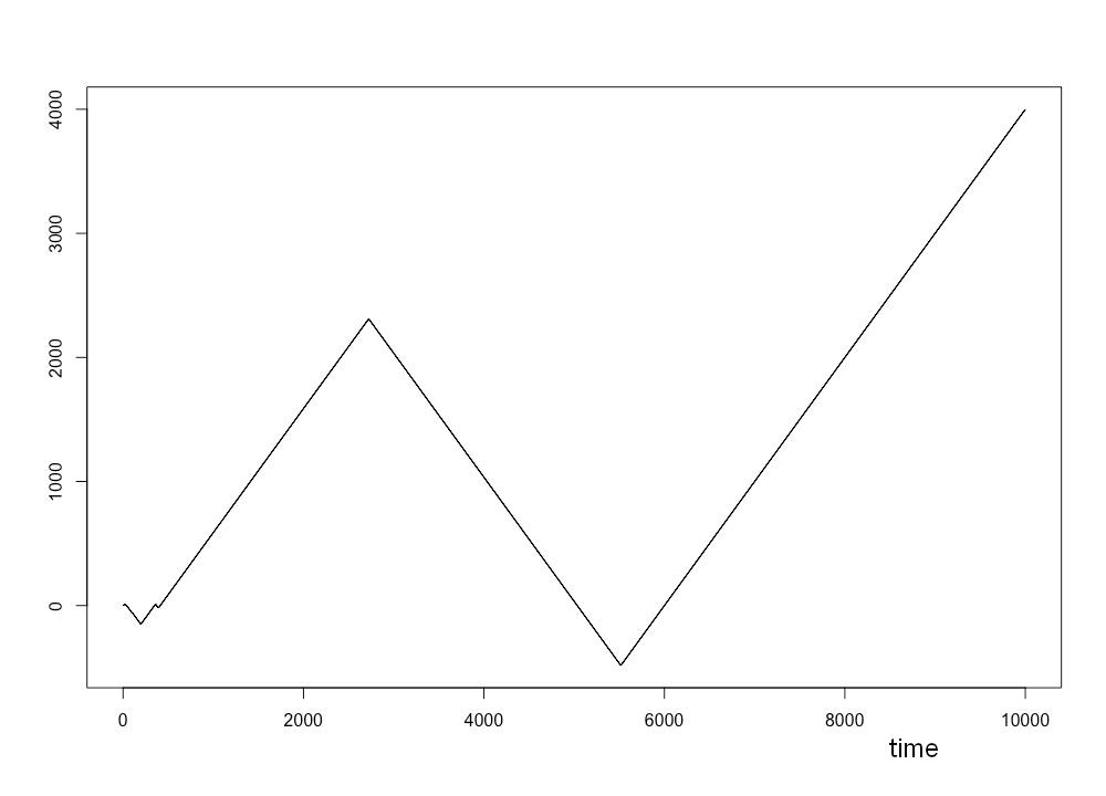
Consider a Poisson point process (PPP) on [0,∞)[0,\infty) with intensity measure ax​d​x\frac{a}{x}\,\mathrm{d}x with a>0a>0. Once the realization is fixed, the value of the process at t≥0t\geq 0 is obtained as follows. Starting with the segment containing tt and going backwards towards the origin, color the first, third, fifth, etc. segments between the points blue. The second, fourth, etc. will be colored red. Given this Poisson intensity, we will have infinitely many segments towards zero (and also towards infinity) almost surely.
Refer to caption
Figure 4. The zigzag process: turning points form a PPP on [0,∞)[0,\infty) with intensity measure ax​d​x\frac{a}{x}\,\mathrm{d}x. (Obtained by simulating SS.)

Let λb​(t)\lambda_{b}(t) and λr​(t)\lambda_{r}(t) denote the Lebesgue measure of the union of blue, resp. red segments between 00 and tt. Then we define the zigzag process XX by

Xt:=W⁡[λb​(t)−λr​(t)],X_{t}:=W[\lambda_{b}(t)-\lambda_{r}(t)],

where WW is a random sign, that is W=−1W=-1 or W=1W=1 with equal probabilities. See Figure 4.

It is easy to check directly that the law of the process is invariant under scaling both axes by the same number.

Remark 11 (One-dimensional marginals).

It is more challenging to check directly that the one-dimensional marginals of the zigzag process are 𝖡𝖾𝗍𝖺⁡(a,a)\mathsf{Beta}(a,a), although this follows immediately from Theorem 4 along with the scaling limit result for the one-dimensional distributions in [7]. Edward Crane has shown us a nice direct proof for this fact though. The interested reader may enjoy trying to find such a proof him/herself.⋄\hfill\diamond

6.2. Preparation II: Approximating the walk with a martingale

We are interested in the scaling limit of the random walk SS, and in particular, whether we have a Donsker-style invariance principle, leading eventually to Brownian motion. Following the general principle that “it always helps to find a martingale”, in this section we investigate the following important, though still somewhat vague, question.

Question 1 (M).

For a given sequence {pn}n≥1\{p_{n}\}_{n\geq 1} is the walk SS “sufficiently close” to some martingale MM?

After Question (M), the next question is of course:

Question 2 (INV.M).

Is there an invariance principle for MM?

Focusing now on Question (M) only, we recall from (1) and (2) the identity ei,j=𝔼⁡(Yj∣Yi)/Yi,e_{i,j}={\mathbb{E}}(Y_{j}\mid Y_{i})/Y_{i}, and that for 1≤i<j<k1\leq i<j<k, ei,j​ej,k=ei,k.e_{i,j}e_{j,k}=e_{i,k}. With the convention ei,i:=𝔼⁡(Yi2)=1e_{i,i}:={\mathbb{E}}(Y^{2}_{i})=1, recall the definition of an=∑i=0∞en,n+ia_{n}=\sum_{i=0}^{\infty}e_{n,n+i} from (7), assuming that the series is convergent (if pn≥1/2p_{n}\geq 1/2 for large nn, then it always is; see below). Then

Mn:=Y1+…​Yn−1+an​YnM_{n}:=Y_{1}+\dots Y_{n-1}+a_{n}Y_{n}

is a martingale. Indeed,

𝔼⁡(Mn+1−Mn∣ℱn)\displaystyle{\mathbb{E}}(M_{n+1}-M_{n}\mid\mathcal{F}_{n}) =𝔼⁡((1−an)​Yn+an+1​Yn+1∣ℱn)\displaystyle={\mathbb{E}}((1-a_{n})Y_{n}+a_{n+1}Y_{n+1}\mid\mathcal{F}_{n})
=(1−an)​Yn+an+1​𝔼​(Yn+1∣Yn)\displaystyle=(1-a_{n})Y_{n}+a_{n+1}{\mathbb{E}}(Y_{n+1}\mid Y_{n})
=[(1−an)+an+1​en,n+1]​Yn,\displaystyle=[(1-a_{n})+a_{n+1}e_{n,n+1}]Y_{n},

which is identically zero, since an+1​en,n+1=an−1a_{n+1}e_{n,n+1}=a_{n}-1, as

an+1​en,n+1=∑i=1∞en,n+1​en+1,n+i=∑i=1∞en,n+i=an−1.a_{n+1}e_{n,n+1}=\sum_{i=1}^{\infty}e_{n,n+1}e_{n+1,n+i}=\sum_{i=1}^{\infty}e_{n,n+i}=a_{n}-1.

Observe also that

𝖵𝖺𝗋⁡(Mn+1−Mn)\displaystyle\mathsf{Var}(M_{n+1}-M_{n}) =𝖵𝖺𝗋⁡((1−an)​Yn+an+1​Yn+1)\displaystyle=\mathsf{Var}\left((1-a_{n})Y_{n}+a_{n+1}Y_{n+1}\right)
=(1−an)2​𝖵𝖺𝗋​(Yn)+an+12​𝖵𝖺𝗋​(Yn+1)+2​(1−an)​an+1​𝖢𝗈𝗏​(Yn,Yn+1)\displaystyle=(1-a_{n})^{2}\mathsf{Var}(Y_{n})+a_{n+1}^{2}\mathsf{Var}(Y_{n+1})+2(1-a_{n})a_{n+1}\mathsf{Cov}(Y_{n},Y_{n+1})
(21) =an+12+(1−an)2+2​(1−an)​an+1​en,n+1=an+12−(1−an)2\displaystyle=a_{n+1}^{2}+(1-a_{n})^{2}+2(1-a_{n})a_{n+1}e_{n,n+1}=a_{n+1}^{2}-(1-a_{n})^{2}
=an+12​[1−en,n+12]=4​an+12​pn+1​qn+1\displaystyle=a_{n+1}^{2}\left[1-e_{n,n+1}^{2}\right]=4a_{n+1}^{2}p_{n+1}q_{n+1}

since 𝖵𝖺𝗋⁡(Yn)=𝔼⁡(Yn2)=1\mathsf{Var}(Y_{n})={\mathbb{E}}(Y_{n}^{2})=1 for each nn.

To understand what we mean by being sufficiently close to a martingale, recall that the rescaled walk Sn{S}^{n} is defined by

Sn​(t):=SZ⁡(n​t)n=MZ⁡(n​t)+(1−aZ⁡(n​t))​YZ⁡(n​t)n,t≥0,{S}^{n}(t):=\frac{S_{Z(nt)}}{\sqrt{n}}=\frac{M_{Z(nt)}+(1-a_{Z(nt)})Y_{Z(nt)}}{\sqrt{n}},\ t\geq 0,

where

Z⁡(n):=inf{m:vm≥n},n≥1,\displaystyle Z(n):=\inf\{m:\ v_{m}\geq n\},\ n\geq 1,

Since |Yk|=1|Y_{k}|=1, if the ana_{n} are not too large, then it suffices to analyze the sequence of the rescaled martingales Mn​(t):=MZ⁡(n​t)nM^{n}(t):=\frac{M_{Z(nt)}}{\sqrt{n}} instead of the sequence of the rescaled random walks. Thus, we have the answer in the affirmative to Question (M), provided that

  1. (a)

    ana_{n} is well-defined;

  2. (b)

    aZ⁡(n)=o⁡(n)a_{Z(n)}=o(\sqrt{n}) (e.g. when ana_{n} remains bounded) as n→∞n\to\infty. (We dropped tt as it is just a constant.)

Proposition 2 (Equivalent conditions for (b)).

Set

σn2:=𝖵𝖺𝗋⁡(Sn).\sigma_{n}^{2}:=\mathsf{Var}(S_{n}).

Since the martingale differences Mi−Mi−1M_{i}-M_{i-1} are uncorrelated and centered, one has

𝖵𝖺𝗋⁡(Mn)=𝔼⁡[(∑i=1n[Mi−Mi−1])2]=∑i=1n𝔼⁡[(Mi−Mi−1)2]=vn,\mathsf{Var}(M_{n})={\mathbb{E}}\left[\left(\sum_{i=1}^{n}[M_{i}-M_{i-1}]\right)^{2}\right]=\sum_{i=1}^{n}{\mathbb{E}}[(M_{i}-M_{i-1})^{2}]=v_{n},

where vnv_{n} is defined by (8) and 𝖵𝖺𝗋⁡(Mi−Mi−1)\mathsf{Var}(M_{i}-M_{i-1}) is given by (6.2). Then the conditions

  • (b.1)

    vn→∞,an=o⁡(vn)v_{n}\to\infty,a_{n}=o\left(\sqrt{v_{n}}\right);

  • (b.2)

    σn→∞,an=o⁡(σn)\sigma_{n}\to\infty,a_{n}=o(\sigma_{n})

are equivalent; and when they are satisfied, vn∼σn\sqrt{v_{n}}\sim\sigma_{n}.

Of course, (𝖻​.1)⇔(𝖻​.2)⇒(𝖻){\sf(b.1)}\Leftrightarrow{\sf(b.2)}\Rightarrow{\sf(b)}. Moreover, if vn→∞v_{n}\to\infty, then the condition an=o⁡(vn)a_{n}=o\left(\sqrt{v_{n}}\right) is in fact equivalent to (b). The proofs of these statements are provided later.⋄\hfill\diamond

To answer Question (INV.M), we refer the invariance principle of Drogin.

Proposition D1972 (Part of Theorem 1 in [6]).

Let (Xi)i≥1(X_{i})_{i\geq 1} be a sequence of square integrable random variables adapted to the filtration (ℱi)i≥1(\mathcal{F}_{i})_{i\geq 1}. Assume that they are martingale differences: 𝔼⁡(Xi∣ℱi−1)=0{\mathbb{E}}(X_{i}\mid\mathcal{F}_{i-1})=0, and that vm:=∑i=1m𝔼⁡(Xi2∣ℱi−1)→∞v_{m}:=\sum_{i=1}^{m}{\mathbb{E}}(X^{2}_{i}\mid\mathcal{F}_{i-1})\to\infty a.s. The processes SS and Sn,n≥1S^{n},\ n\geq 1 by S⁡(vm)=∑i=1mXi,S⁡(0):=0,S(v_{m})=\sum_{i=1}^{m}X_{i},\ S(0):=0, and by Sn​(t):=S⁡(n​t)/n,t≥0S^{n}(t):=S(nt)/\sqrt{n},\ t\geq 0, using linear interpolation between integer times. Then the following are equivalent:

  • (i)

    If ϵ>0\epsilon>0, then

    (22) 1n∑i=1Z⁡(n)Xi21{Xi2>nϵ}→L10asn→∞.\frac{1}{n}\sum_{i=1}^{Z(n)}X_{i}^{2}1_{\{X_{i}^{2}>n\epsilon\}}\to_{L_{1}}0\quad\text{as}\ n\to\infty.
  • (ii)

    As n→∞n\to\infty, the law of SnS^{n} converges to the Wiener measure and

    vZ⁡(n)n→L11.\frac{v_{Z(n)}}{n}\to_{L_{1}}1.

Note that, in our setting, both vmv_{m} and Z⁡(n)Z(n) are deterministic. To summarize the discussion of Question(M) and (INV.M) above, in our setting, once the limit process is Brownian motion, we need to check the following conditions,

  1. (a)

    ana_{n} is well-defined;

  2. (b)

    aZ⁡(n)=o⁡(n)a_{Z(n)}=o(\sqrt{n}), or equivalently, an=o⁡(σn)a_{n}=o(\sigma_{n}) (given vn→∞v_{n}\rightarrow\infty), as n→∞n\to\infty.

  3. (c)

    vn→∞v_{n}\rightarrow\infty and (22) holds.

Here (a), (b) guarantee (M) affirmative , and (c) guarantees (IN.V) affirmative.

6.3. Some specific cases

The first two cases we are looking at are in the cooling regime, the last one is in the heating regime. We will use the conditions discussed in the last paragraph in Proposition 2.

6.3.1. Cooling, critical

Let pn=c/np_{n}=c/n for large nn. If c≥1/2c\geq 1/2, then (a) fails to hold, because then an=∞a_{n}=\infty. Otherwise ana_{n} is of order n1−2​cn^{1-2c}, and vn\sqrt{v_{n}} is of the same order, and thus (b) fails to hold. In both cases, the answer to Question (M) is negative.

6.3.2. Cooling, subcritical

Let pn≤1/2p_{n}\leq 1/2 for all44 4 We may assume this without the loss of generality, as the validity of the invariance principle does not depend on a finite number of terms. n≥1n\geq 1 and pn=c/nγp_{n}=c/n^{\gamma} for nn large, where 0<γ<10<\gamma<1. In this case the answers to (M) and to (INV.M) are both in the affirmative, and one can compute that an=nγ2​c​(1+o⁡(1))a_{n}=\frac{n^{\gamma}}{2c}(1+o(1)).

6.3.3. Cooling, subcritical; the necessity of lim infn→∞pnpn+1>0\liminf\limits_{n\rightarrow\infty}\frac{p_{n}}{p_{n+1}}>0

One can see that assumption (a) in Theorem 4(4) guarantees that

lim infn→∞pnpn+1>0.\liminf_{n\to\infty}\frac{p_{n}}{p_{n+1}}>0.

The following example shows indeed the necessity of this bound, that is, by showing that the property that an=o⁡(vn)a_{n}=o(v_{n}) can break down if this l​i​m​i​n​fliminf is zero. Indeed, let

pi:=ln⁡k2⋅k! for k!<i≤(k+1)!,k=1,2,….p_{i}:=\frac{\ln k}{2\cdot k!}\text{\ \ for }k!<i\leq(k+1)!,\quad k=1,2,\dots.

Then

∏i=k!+1(k+1)!(1−2​pi)=(1−ln⁡kk!)k⋅k!=(1+o⁡(1))​e−k​ln⁡k=1+o⁡(1)kk\prod_{i=k!+1}^{(k+1)!}(1-2p_{i})=\left(1-\frac{\ln k}{k!}\right)^{k\cdot k!}=(1+o(1))e^{-k\ln k}=\frac{1+o(1)}{k^{k}}

and ∑k(k+1)!−k!kk<∞\sum_{k}\frac{(k+1)!-k!}{k^{k}}<\infty, so ana_{n} is well-defined. Moreover,

am!\displaystyle a_{m!} =∑i=0∞em!,m!+i≥1+∑i=1(m+1)!−m!(1−2​pm!+1)​…​(1−2​pm!+i)\displaystyle=\sum_{i=0}^{\infty}e_{m!,m!+i}\geq 1+\sum_{i=1}^{(m+1)!-m!}(1-2p_{m!+1})\dots(1-2p_{m!+i})
=1+[1−ln⁡mm!]+[1−ln⁡mm!]2+⋯+[1−ln⁡mm!](m+1)!−m!\displaystyle=1+\left[1-\frac{\ln m}{m!}\right]+\left[1-\frac{\ln m}{m!}\right]^{2}+\dots+\left[1-\frac{\ln m}{m!}\right]^{(m+1)!-m!}
=1−O⁡(e−m​ln⁡m)1−(1−ln⁡mm!)=(1+o⁡(1))​m!ln⁡m.\displaystyle=\frac{1-O\left(e^{-m\ln m}\right)}{1-\left(1-\frac{\ln m}{m!}\right)}=(1+o(1))\,\frac{m!}{\ln m}.

At the same time,

vm!4\displaystyle\frac{v_{m!}}{4} =∑i=1m!ai2​pi​qi=∑k=0m−1∑i=k!+1(k+1)!ai2​pi​qi≤∑k=0m−1[∑i=k!+1(k+1)!ai2​ln⁡kk!]\displaystyle=\sum_{i=1}^{m!}a_{i}^{2}p_{i}q_{i}=\sum_{k=0}^{m-1}\sum_{i=k!+1}^{(k+1)!}a_{i}^{2}p_{i}q_{i}\leq\sum_{k=0}^{m-1}\left[\sum_{i=k!+1}^{(k+1)!}a_{i}^{2}\,\frac{\ln k}{k!}\right]
≤∑k=0m−1(1+o⁡(1))​k!ln⁡k≤(1+o​(1))​(m−1)!ln⁡(m−1)≤1+o⁡(1)m⋅m!ln⁡m=o⁡(am!2),\displaystyle\leq\sum_{k=0}^{m-1}(1+o(1))\frac{k!}{\ln k}\leq\frac{(1+o(1))(m-1)!}{\ln(m-1)}\leq\frac{1+o(1)}{m}\cdot\frac{m!}{\ln m}=o\left(a_{m!}^{2}\right),

since for k!<i≤(k+1)!k!<i\leq(k+1)!,

ai\displaystyle a_{i} ≤∑j=0(k+1)!−k![1−ln⁡kk!]j+[1−ln⁡kk!](k+1)!−k!⋅∑j=0(k+2)!−(k+1)![1−ln⁡(k+1)(k+1)!]j\displaystyle\leq\sum_{j=0}^{(k+1)!-k!}\left[1-\frac{\ln k}{k!}\right]^{j}+\left[1-\frac{\ln k}{k!}\right]^{(k+1)!-k!}\cdot\sum_{j=0}^{(k+2)!-(k+1)!}\left[1-\frac{\ln(k+1)}{(k+1)!}\right]^{j}
+[1−ln⁡kk!](k+1)!−k!⋅[1−ln⁡(k+1)(k+1)!](k+1)!−k!⋅∑j=0(k+3)!−(k+2)![1−ln⁡(k+2)(k+2)!]j+…\displaystyle+\left[1-\frac{\ln k}{k!}\right]^{(k+1)!-k!}\cdot\left[1-\frac{\ln(k+1)}{(k+1)!}\right]^{(k+1)!-k!}\cdot\sum_{j=0}^{(k+3)!-(k+2)!}\left[1-\frac{\ln(k+2)}{(k+2)!}\right]^{j}+\dots
≤(1+o⁡(1))​k!ln⁡k+e−k​ln⁡k​(k+2)!+e−k​ln⁡k​e−(k+1)​ln⁡(k+1)​(k+3)!+…\displaystyle\leq(1+o(1))\frac{k!}{\ln k}+e^{-k\ln k}(k+2)!+e^{-k\ln k}e^{-(k+1)\ln(k+1)}(k+3)!+\dots
≤(1+o⁡(1))​k!ln⁡k+(k+2)!kk+(k+3)!(k+1)m+1+(k+4)!(k+2)k+2+…=(1+o⁡(1))​k!ln⁡k.\displaystyle\leq(1+o(1))\frac{k!}{\ln k}+\frac{(k+2)!}{k^{k}}+\frac{(k+3)!}{(k+1)^{m+1}}+\frac{(k+4)!}{(k+2)^{k+2}}+...=(1+o(1))\frac{k!}{\ln k}.

At the same time it is worth noting that with these pip_{i}’s, the assumption (4)(a) in Theorem 4 is violated too, since for i=(m+1)!i=(m+1)!, one has

i​pi=(m+1)!​p(m+1)!=(m+1)!​ln⁡m2⋅m!=[12+m2]​ln⁡m,\displaystyle ip_{i}=(m+1)!\,p_{(m+1)!}=(m+1)!\frac{\ln m}{2\cdot m!}=\left[\frac{1}{2}+\frac{m}{2}\right]\ln m,

while

(i+1)​pi+1=[(m+1)!+1]​ln⁡(m+1)2⋅(m+1)!=[12+o⁡(1)]​ln⁡m≪i​pi.(i+1)p_{i+1}=\left[(m+1)!+1\right]\frac{\ln(m+1)}{2\cdot(m+1)!}=\left[\frac{1}{2}+o(1)\right]\ln m\ll ip_{i}.

6.3.4. (Heating)

Let pn=1−qnp_{n}=1-q_{n} and qn→0q_{n}\to 0 but ∑qn=∞\sum q_{n}=\infty. We have

an=1+∑i=1∞(−1)i​(1−2​qn+1)​(1−2​qn+2)​…​(1−2​qn+i),a_{n}=1+\sum_{i=1}^{\infty}(-1)^{i}(1-2q_{n+1})(1-2q_{n+2})\dots(1-2q_{n+i}),

and, since 1−2​pn=2​qn−1<01-2p_{n}=2q_{n}-1<0 for large nn, using the Leibniz criterion, along with the assumption that ∑qn=∞\sum q_{n}=\infty, it follows that ana_{n} is well defined. The validity of the martingale approximation follows from the fact that an≤1a_{n}\leq 1 but vn→∞v_{n}\to\infty; see the proof of Theorem 3.

6.4. Proof of Theorem 1

Clearly, if pi=1/2p_{i}=1/2 for some i∈ℕi\in{\mathbb{N}} then the process “gets symmetrized” from time ii on (and ρ=0\rho=0), and the statement is trivial. We will thus assume in the rest of the proof that pi≠1/2,∀i∈ℕp_{i}\neq 1/2,\ \forall i\in{\mathbb{N}}.

Furthermore, we will handle the conditional probability ℙ(⋅∣Y1=1){\mathbb{P}}(\cdot\mid Y_{1}=1) only, the argument for ℙ(⋅∣Y1=−1){\mathbb{P}}(\cdot\mid Y_{1}=-1) is similar. In terms of the WiW_{i}, one has Yn:=(−1)∑i=1nWi,Y_{n}:=(-1)^{\sum_{i=1}^{n}W_{i}}, where W1,W2,W3,…W_{1},W_{2},W_{3},... are independent Bernoulli variables with parameters p1,p2,p3,…p_{1},p_{2},p_{3},..., respectively and we will handle the p1=0p_{1}=0 (i.e. W1≡0W_{1}\equiv 0) case. In particular, ∏i=1n(1−2​pi)=∏i=2n(1−2​pi).\prod_{i=1}^{n}(1-2p_{i})=\prod_{i=2}^{n}(1-2p_{i}).

Let xn:=ℙ⁡(Yn=1)x_{n}:={\mathbb{P}}(Y_{n}=1). We have the recursion

xn+1\displaystyle x_{n+1} =\displaystyle= pn​(1−xn)+(1−pn)​xn,n≥1;\displaystyle p_{n}(1-x_{n})+(1-p_{n})x_{n},\ n\geq 1;
x1\displaystyle x_{1} =\displaystyle= 1,\displaystyle 1,

and the substitution yn:=xn−1/2y_{n}:=x_{n}-1/2 yields yn+1=(1−2​pn)​yny_{n+1}=(1-2p_{n})y_{n} with y1=1/2y_{1}=1/2. Hence,

(23) yn+1=12​∏i=1n(1−2​pi).y_{n+1}=\frac{1}{2}\prod_{i=1}^{n}(1-2p_{i}).

Case 1: N=∞N=\infty. We have to prove that xnx_{n} converges to 1/2 or has no limit, according to whether min⁡(pi,qi)\min(p_{i},q_{i}) is summable or not.

Let Nn:=card⁡{i≤n:pi>1/2};N_{n}:=\mathrm{card}\{i\leq n:\ p_{i}>1/2\}; then limn→∞Nn=∞.\lim_{n\to\infty}N_{n}=\infty. Since

min⁡(pi,qi)={pi.if ​pi<1/2;qi=(1−pi),if ​pi>1/2,\min(p_{i},q_{i})=\begin{cases}p_{i}.&\text{if }p_{i}<1/2;\\ q_{i}=(1-p_{i}),&\text{if }p_{i}>1/2,\end{cases}

we have

∏i=1n(1−2​pi)=∏i≤n,pi≤1/2(1−2​pi)×∏i≤n,pi>1/2(1−2​pi)\displaystyle\prod_{i=1}^{n}(1-2p_{i})=\prod_{i\leq n,p_{i}\leq 1/2}(1-2p_{i})\times\prod_{i\leq n,p_{i}>1/2}(1-2p_{i})
=(−1)Nn​∏i≤n,pi≤1/2(1−2​pi)×∏i≤n,pi>1/2(1−2​qi)=(−1)Nn​∏i=1n(1−2​min⁡(pi,qi)).\displaystyle=(-1)^{N_{n}}\prod_{i\leq n,p_{i}\leq 1/2}(1-2p_{i})\times\prod_{i\leq n,p_{i}>1/2}(1-2q_{i})=(-1)^{N_{n}}\prod_{i=1}^{n}(1-2\min(p_{i},q_{i})).

Given that limn(−1)Nn\lim_{n}(-1)^{N_{n}} does not exist, there are two cases:

(i) the right-hand side converges because the product (without the (−1)Nn(-1)^{N_{n}} factor) converges to zero and mixing holds (OPEN∑i=1∞min⁡(pi,qi)=∞)\sum_{i=1}^{\infty}\min(p_{i},q_{i})=\infty), in which case limnyn=0\lim_{n}y_{n}=0 and limnxn=1/2\lim_{n}x_{n}=1/2.

(ii) the right-hand side has no limit and mixing does not hold in which case yny_{n} (hence xnx_{n}) has no limit.

Case 2: N<∞N<\infty. Let us assume first that N=0N=0, that is, pi<1/2,i≥1p_{i}<1/2,i\geq 1. If ∑i=1∞pi=∞\sum_{i=1}^{\infty}p_{i}=\infty then in (23) we have ∏i=1n(1−2​pi)↓0\prod_{i=1}^{n}(1-2p_{i})\downarrow 0, implying limnyn=0\lim_{n}y_{n}=0 and limnxn=1/2\lim_{n}x_{n}=1/2. If ∑i=1∞pi<∞\sum_{i=1}^{\infty}p_{i}<\infty, then ρ=∏i=1∞(1−2​pi)>0\rho=\prod_{i=1}^{\infty}(1-2p_{i})>0 and limnyn=12​ρ\lim_{n}y_{n}=\frac{1}{2}\rho, that is, limnxn=12​(1+ρ).\lim_{n}x_{n}=\frac{1}{2}(1+\rho).

In the general case, for large ii, min⁡(pi,qi)=pi<1/2\min(p_{i},q_{i})=p_{i}<1/2, and mixing is tantamount to ∑i=1∞pi=∞\sum_{i=1}^{\infty}p_{i}=\infty. The proof is very similar as before, using the fact that the product has positive terms for large enough indices.

6.5. Proof of Theorem 2

The martingale method is applicable in this case too. Indeed, direct computation gives an=12​pa_{n}=\frac{1}{2p}, ∀n\forall n and vn=∑𝑛​4​ai2​pi​qi=1−pp​n.v_{n}=\overset{n}{\sum}4a_{i}^{2}p_{i}q_{i}=\frac{1-p}{p}n. Hence an=o⁡(vn)a_{n}=o(\sqrt{v_{n}}), ai2​ξi2a^{2}_{i}\xi^{2}_{i} are bounded, so (22) holds, and thus we can apply Proposition D1972, yielding the answer to (INV.M) in the affirmative.∎

6.6. Proof of Theorem 3

First we will prove the statement under the more restrictive assumption that

(24) lim supn→∞qn+1qn<∞,\displaystyle\limsup_{n\to\infty}\frac{q_{n+1}}{q_{n}}<\infty,

and then we upgrade it for showing the statement under the condition appearing in the theorem.

6.6.1. STEP 1

We start with a simple lemma.

Lemma 1.

Assume that for the non-negative sequence (qn)(q_{n}), such that

  • •

    qn→0q_{n}\to 0,

  • •

    ∑nqn=∞\sum_{n}q_{n}=\infty,

  • •

    the condition (24) holds.

Then lim infn→∞an>0\liminf_{n\to\infty}a_{n}>0, where the ana_{n} are defined by (7). Moreover, if limn→∞qn+1qn=1,\displaystyle\lim_{n\to\infty}\frac{q_{n+1}}{q_{n}}=1, then limn→∞an=1/2\displaystyle\lim_{n\to\infty}a_{n}=1/2.

Remark 12.

The condition that qn→0q_{n}\rightarrow 0 is really necessary in Lemma 1. Indeed, fix c1,c2>0c_{1},c_{2}>0, c1≠c2c_{1}\neq c_{2} and let qn=c1/nq_{n}=c_{1}/n if nn is odd and qn=c2/nq_{n}=c_{2}/n if nn is even. Then qn+1/qn↛1q_{n+1}/q_{n}\not\to 1, though (24) still holds. In this case an↛1/2a_{n}\not\to 1/2, rather (as it is not hard to show) limk→∞a2​k=c1c1+c2≠c2c1+c2=limk→∞a2​k+1\displaystyle\lim_{k\to\infty}a_{2k}=\frac{c_{1}}{c_{1}+c_{2}}\neq\frac{c_{2}}{c_{1}+c_{2}}=\lim_{k\to\infty}a_{2k+1}. ⋄\hfill\diamond

Proof.

Fix some nn, and for m≥nm\geq n let

wm=∏j=n+1m(1−2​qj),m>n,wn=1,w_{m}=\prod_{j=n+1}^{m}(1-2q_{j}),\ m>n,\quad w_{n}=1,

and note that wm↓0w_{m}\downarrow 0 as m→∞m\to\infty due to ∑qi=∞\sum q_{i}=\infty. Then

an=∑i=0∞(−1)i​wn+i=∑k=0∞(wn+2​k−wn+2​k+1)=∑k=0∞2​qn+2​k+1​wn+2​k.a_{n}=\sum_{i=0}^{\infty}(-1)^{i}w_{n+i}=\sum_{k=0}^{\infty}\left(w_{n+2k}-w_{n+2k+1}\right)=\sum_{k=0}^{\infty}2q_{n+2k+1}\,w_{n+2k}.

Now take any finite c>lim supnqn+1/qnc>\limsup_{n}q_{n+1}/q_{n}, and assume that nn is so large that the quantity qℓ+1/qℓ<cq_{\ell+1}/q_{\ell}<c for all ℓ≥n\ell\geq n. Then

(25) wn+2​k−wn+2​k+2\displaystyle w_{n+2k}-w_{n+2k+2} =2​(qn+2​k+1+qn+2​k+2−2​qn+2​k+1​qn+2​k+2)⋅wn+2​k\displaystyle=2(q_{n+2k+1}+q_{n+2k+2}-2q_{n+2k+1}q_{n+2k+2})\cdot w_{n+2k}
≤2​(qn+2​k+1+qn+2​k+2)⋅wn+2​k≤(1+c)⋅2​qn+2​k+1​wn+2​k.\displaystyle\leq 2(q_{n+2k+1}+q_{n+2k+2})\cdot w_{n+2k}\leq(1+c)\cdot 2q_{n+2k+1}w_{n+2k}.

As a result,

(1+c)​an=∑k=0∞(1+c)⋅2​qn+2​k+1​wn+2​k≥∑k=0∞(wn+2​k−wn+2​k+2)=wn=1>0,(1+c)a_{n}=\sum_{k=0}^{\infty}(1+c)\cdot 2q_{n+2k+1}\,w_{n+2k}\geq\sum_{k=0}^{\infty}\left(w_{n+2k}-w_{n+2k+2}\right)=w_{n}=1>0,

where the telescopic sum converges due to the fact that wm→0w_{m}\to 0. Since c>lim supnqn+1/qnc>\limsup_{n}q_{n+1}/q_{n} is arbitrary, we can even conclude that

(26) lim infn→∞an≥11+lim supn→∞qn+1/qn.\displaystyle\liminf_{n\to\infty}a_{n}\geq\frac{1}{1+\limsup_{n\to\infty}q_{n+1}/q_{n}}.

To prove the second part of the claim, observe that from (26) we already have lim infnan≥1/2\liminf_{n}a_{n}\geq 1/2. To show the counterpart of this, fix an arbitrary ε>0\varepsilon>0 and let nn be so large that qn+2​k+2qn+2​k+1≥1−ε/2\frac{q_{n+2k+2}}{q_{n+2k+1}}\geq 1-\varepsilon/2 and qn+2​k+2≤ε/4q_{n+2k+2}\leq\varepsilon/4 for all k≥0k\geq 0. Then

qn+2​k+1+qn+2​k+2−2​qn+2​k+1​qn+2​k+2=(1+qn+2​k+2qn+2​k+1−2​qn+2​k+2)​qn+2​k+1\displaystyle q_{n+2k+1}+q_{n+2k+2}-2q_{n+2k+1}q_{n+2k+2}=\left(1+\frac{q_{n+2k+2}}{q_{n+2k+1}}-2q_{n+2k+2}\right)q_{n+2k+1}
≥(2−ε)⋅qn+2​k+1,\displaystyle\geq(2-\varepsilon)\cdot q_{n+2k+1},

given that qn+2​k+2qn+2​k+1→1\displaystyle\frac{q_{n+2k+2}}{q_{n+2k+1}}\to 1 and qn+2​k+2→0q_{n+2k+2}\to 0. Hence (see (25))

wn+2​k−wn+2​k+2≥(2−ε)⋅2​qn+2​k+1​wn+2​kw_{n+2k}-w_{n+2k+2}\geq(2-\varepsilon)\cdot 2q_{n+2k+1}w_{n+2k}

and

(2−ε)​an=∑k=0∞(2−ε)⋅2​qn+2​k+1​wn+2​k≤∑k=0∞(wn+2​k−wn+2​k+2)=wn=1.(2-\varepsilon)a_{n}=\sum_{k=0}^{\infty}(2-\varepsilon)\cdot 2q_{n+2k+1}\,w_{n+2k}\leq\sum_{k=0}^{\infty}\left(w_{n+2k}-w_{n+2k+2}\right)=w_{n}=1.

Since ε>0\varepsilon>0 is arbitrary, we conclude that lim supnan≤1/2\limsup_{n}a_{n}\leq 1/2, which completes the proof. ∎

We now continue the proof of the theorem under the assumption that (24) holds.

Proof of Theorem 3 (a):
Noting that all conditions at the end of Section 6.2 to Question(M),(INV.M) are in the affirmative (as ana_{n} is well-defined and stays bounded), except (22). Since in our case Xi=ai​ξi​Yi−1X_{i}=a_{i}\xi_{i}Y_{i-1} and |Yi|=1|Y_{i}|=1, what we need is to show that

(27) limn→∞1n∑i=1Z⁡(n)ai2ξi2𝟏{ai2ξi2>nϵ}=0.\lim_{n\to\infty}\frac{1}{n}\sum_{i=1}^{Z(n)}a_{i}^{2}\xi_{i}^{2}\mathbf{1}_{\{a_{i}^{2}\xi_{i}^{2}>n\epsilon\}}=0.

(Note that Z⁡(n)Z(n) in our case it is deterministic, and so is vmv_{m}.) Since

ξi2=[(−1)Wi+(2​pi−1)]2≤4, and ​|ai|≤1,\xi_{i}^{2}=[(-1)^{W_{i}}+(2p_{i}-1)]^{2}\leq 4,\text{ and }|a_{i}|\leq 1,

as aia_{i} is a Leibniz series, all but finitely many terms in the sum in (27) are zero, proving (27). We conclude that (22) holds.

Next, a direct computation shows that vm=4​∑i=1mai2​pi​qi.v_{m}=4\sum_{i=1}^{m}a_{i}^{2}p_{i}q_{i}. Then

limm→∞vm=∑i=1∞4​ai2​pi​qi=∞\lim_{m\to\infty}v_{m}=\sum_{i=1}^{\infty}4a_{i}^{2}p_{i}q_{i}=\infty

follows from Lemma 1 and from the assumptions pn→1p_{n}\to 1 and ∑qn=∞\sum q_{n}=\infty. The proof of (a) is thus complete.

Proof of Theorem 3 (b): First, we prove that Λn2=∑i=1nai2​ξi2→∞\Lambda_{n}^{2}=\sum_{i=1}^{n}a_{i}^{2}\xi_{i}^{2}\to\infty. Recall that ξi=(−1)Wi−E​(−1)Wi=2​pi−1+(−1)Wi\xi_{i}=(-1)^{W_{i}}-E(-1)^{W_{i}}=2p_{i}-1+(-1)^{W_{i}} satisfies 𝔼​ξi2=𝖵𝖺𝗋⁡((−1)Wi)=4​pi​qi{\mathbb{E}}\xi_{i}^{2}=\mathsf{Var}((-1)^{W_{i}})=4p_{i}q_{i}. Let also Ui:=ai2​ξi2∈[0,4]U_{i}:=a_{i}^{2}\xi_{i}^{2}\in[0,4].

Since the WiW_{i} are independent, so are the ξi\xi_{i}, and hence, for Λn2\Lambda_{n}^{2}, the Three Series Theorem applies: the non-negative series ∑iUi\sum_{i}U_{i} diverges if for some A>0A>0, ∑i𝔼⁡[Ui;|Ui|≤A]\sum_{i}{\mathbb{E}}[U_{i};|U_{i}|\leq A] diverges. But for A>4A>4,

∑i𝔼⁡[Ui;|Ui|≤A]=∑i𝔼⁡(Ui)=∑iai2​pi​qi=∞,\sum_{i}{\mathbb{E}}[U_{i};\ |U_{i}|\leq A]=\sum_{i}{\mathbb{E}}(U_{i})=\sum_{i}a_{i}^{2}p_{i}q_{i}=\infty,

as aia_{i} is bounded away from zero, pi→1p_{i}\to 1 and ∑qi=∞.\sum q_{i}=\infty.

Alternatively, let ϵ>0\epsilon>0. Then pi→1p_{i}\to 1 and ∑qi=∞\sum q_{i}=\infty along with the second Borel-Cantelli lemma guarantee that ξi=2​pi−1+(−1)Wi≥2−ϵ\xi_{i}=2p_{i}-1+(-1)^{W_{i}}\geq 2-\epsilon for infinitely many ii’s almost surely. We are done because the aia_{i} are bounded away from zero.

For the second statement, by using Chebyshev’s inequality, it is enough to show that

(28) limn→∞𝖵𝖺𝗋⁡(Λn2)(𝔼​Λn2)2=0.\displaystyle\lim_{n\to\infty}\frac{\mathsf{Var}(\Lambda_{n}^{2})}{({\mathbb{E}}\Lambda_{n}^{2})^{2}}=0.

Since an,pn,qn∈[0,1]a_{n},p_{n},q_{n}\in[0,1],

(29) 𝖵𝖺𝗋⁡(Λn2)=4​∑i=1nai4​pi​qi​(pi−qi)2≤4​∑i=1nqi.\displaystyle\mathsf{Var}(\Lambda^{2}_{n})=4\sum_{i=1}^{n}a_{i}^{4}p_{i}q_{i}(p_{i}-q_{i})^{2}\leq 4\sum_{i=1}^{n}q_{i}.

Moreover, for large nn’s,

(30) 𝔼​Λn2=vn=4​∑i=1nai2​pi​qi≥c​∑i=1nqi\displaystyle{\mathbb{E}}\Lambda_{n}^{2}=v_{n}=4\sum_{i=1}^{n}a_{i}^{2}\,p_{i}\,q_{i}\geq c\sum_{i=1}^{n}q_{i}

for some c>0c>0, since lim infi→∞ai>0\displaystyle\liminf_{i\to\infty}a_{i}>0 by Lemma 1 and pi→1p_{i}\to 1. Given that ∑i=1nqi→∞\sum_{i=1}^{n}q_{i}\to\infty, (29) and (30) together yield (28), thus completing the proof of the statement. \hfill\qed

6.6.2. STEP 2

We now upgrade the result obtained in STEP 1, by dropping the restriction that (24) holds. We need the following

Lemma 2 (Comparison with “regular” sequences).

Let 0≤qn≤1/2,n≥10\leq q_{n}\leq 1/2,\ n\geq 1.

(i) Assume that there exists a sequence qk∗→0q^{*}_{k}\to 0 such that qn∗q^{*}_{n} is not summable, regular, in the sense that (24) holds, and qn≤qn∗q_{n}\leq q^{*}_{n} for even nn, while qn≥qn∗q_{n}\geq q^{*}_{n} for odd nn. Then lim infk→∞a2​k>0\displaystyle\liminf_{k\to\infty}a_{2k}>0.

(ii) Assume that there exists a sequence q~k→0\tilde{q}_{k}\to 0 such that q~n\tilde{q}_{n} is not summable, regular in the sense that (24) holds, and qn≤q~nq_{n}\leq\tilde{q}_{n} for odd nn, while qn≥q~nq_{n}\geq\tilde{q}_{n} for even nn. Then lim infk→∞a2​k+1>0\displaystyle\liminf_{k\to\infty}a_{2k+1}>0.

Proof of Lemma 2.

Since 0≤qn≤1/20\leq q_{n}\leq 1/2 for n≥1n\geq 1, it is easy to check the following (for example by observing that for k>nk>n, the coefficients of qkq_{k} in ana_{n} form a Leibniz series as well):

  • •

    Let n=2​kn=2k. Then ana_{n} is decreasing55 5 The terms increasing and decreasing are not used in the strict sense. in all qiq_{i} for which ii is even and increasing in all qiq_{i} for which ii is odd.

  • •

    Let n=2​k+1n=2k+1. Then ana_{n} is increasing in all qiq_{i} for which ii is even and decreasing in all qiq_{i} for which ii is odd.

Turning to the proof of (i) (a similar proof works for (ii), which we omit), note that, because of its monotonicity and non-summability (use I=∞I=\infty and q2​k∗≥q2​kq^{*}_{2k}\geq q_{2k}), STEP 1 yields that (qn∗)(q^{*}_{n}) is such that lim infan>0\liminf a_{n}>0, and in particular, lim infka2​k>0\liminf_{k}a_{2k}>0. Hence, by the first bullet point above, lim infka2​k>0\liminf_{k}a_{2k}>0 also for (qn)(q_{n}), proving (i). ∎

Proof of Theorem 3.

First, without the loss of generality, we assume that m0=1m_{0}=1 (changing a finite number of terms does not change the validity of the invariance principle). Similarly, we may and will assume that qn≤1/2q_{n}\leq 1/2 for all n≥1n\geq 1, as we assume anyway that qn→0q_{n}\to 0.

We only need that vn=4​∑i=1nai2​pi​qi→∞,v_{n}=4\sum_{i=1}^{n}a_{i}^{2}\,p_{i}\,q_{i}\to\infty, what is left is very similar to STEP 1. This will follow from pn→1p_{n}\to 1 and Assumption 2, provided that either lim infka2​k>0\liminf_{k}a_{2k}>0 or lim infka2​k+1>0\liminf_{k}a_{2k+1}>0. By Lemma 2, it is sufficient to construct either a sequence (qn∗)(q_{n}^{*}) or a sequence (q~n)(\tilde{q}_{n}) satisfying the properties in the lemma. These sequences will be automatically divergent, given Assumption 2 and that (qn∗)(q^{*}_{n}) resp. (q~n)(\tilde{q}_{n}) dominate (qn)(q_{n}) for even resp. odd nn’s. Now, assume for example (9) (assuming (10) leads to a similar argument). Define

q~2​m:=C​max⁡{q2​ℓ+1,ℓ≥m},m≥1;\displaystyle\tilde{q}_{2m}:=C\max\{q_{2\ell+1},\ell\geq m\},\ m\geq 1;
q~2​m+1:=max⁡{q2​ℓ+1,ℓ≥m},m≥0.\displaystyle\tilde{q}_{2m+1}:=\max\{q_{2\ell+1},\ell\geq m\},\ m\geq 0.

Then (q~n)(\tilde{q}_{n}) is regular because q~n+1q~n≤max⁡{C−1,C}\frac{\tilde{q}_{n+1}}{\tilde{q}_{n}}\leq\max\{C^{-1},C\} for all n≥1n\geq 1, and trivially q2​m≥q~2​mq_{2m}\geq\tilde{q}_{2m} and q~2​m+1≥q2​m+1\tilde{q}_{2m+1}\geq q_{2m+1}. Hence, lim infka2​k+1>0\liminf_{k}a_{2k+1}>0 by Lemma 2(ii). ∎

Remark 13 (One of the two subsequences can be arbitrary).

Chose an arbitrary “odd” subsequence, satisfying the conditions that it tends to zero and yet not summable. Then take a sufficiently large “even” subsequence that dominates it in the sense of (9), but still tends to zero (for example, let q2​n:=1/2​nq_{2n}:=1/\sqrt{2n} and q2​n+1:=1/(2​n+1)q_{2n+1}:=1/(2n+1)). Then (9) holds, while the condition lim supnqn+1/qn<∞\limsup_{n}q_{n+1}/q_{n}<\infty (cf. (24) in the proof) fails to hold, as limnq2​n/q2​n+1=∞\lim_{n}q_{2n}/q_{2n+1}=\infty.

By the same token, one can first chose an arbitrary non-summable “even” sequence, with the terms tending to zero and then a dominating “odd” one.⋄\hfill\diamond

6.7. Proof of Proposition 2

Recall that Sn=Mn+(1−an)​YnS_{n}=M_{n}+(1-a_{n})Y_{n}, hence

𝖵𝖺𝗋⁡(Sn)=𝖵𝖺𝗋⁡(Mn)+(1−an)2+2​(1−an)​𝖢𝗈𝗏​(Mn,Yn),\mathsf{Var}(S_{n})=\mathsf{Var}(M_{n})+(1-a_{n})^{2}+2(1-a_{n})\mathsf{Cov}(M_{n},Y_{n}),

where, by Cauchy-Schwarz, |𝖢𝗈𝗏⁡(Mn,Yn)|≤𝔼⁡(Mn2)=vn|\mathsf{Cov}(M_{n},Y_{n})|\leq\sqrt{{\mathbb{E}}(M_{n}^{2})}=\sqrt{v_{n}}, so

σn2−vn=(1−an)​(1−an+2​𝖢𝗈𝗏​(Mn,Yn))=(1−an)​(1−an+An​vn),\displaystyle\sigma_{n}^{2}-v_{n}=(1-a_{n})(1-a_{n}+2\mathsf{Cov}(M_{n},Y_{n}))=(1-a_{n})(1-a_{n}+A_{n}\sqrt{v_{n}}),

where |An|≤1|A_{n}|\leq 1. Then

σn2vn−1=1−anvn⋅(1−anvn+An),\frac{\sigma^{2}_{n}}{v_{n}}-1=\frac{1-a_{n}}{\sqrt{v_{n}}}\cdot\left(\frac{1-a_{n}}{\sqrt{v_{n}}}+A_{n}\right),

if vn→∞v_{n}\to\infty and an=o⁡(vn)a_{n}=o(\sqrt{v_{n}}) as n→∞n\to\infty, hence vn∼σn\sqrt{v_{n}}\sim\sigma_{n} follows.

Similarly, we have

1−vnσn2=1−anσn​(1−anσn+An​vn/σn).1-\frac{v_{n}}{\sigma_{n}^{2}}=\frac{1-a_{n}}{\sigma_{n}}\left(\frac{1-a_{n}}{\sigma_{n}}+A_{n}\sqrt{v_{n}}/\sigma_{n}\right).

Using the shorthands wn:=vnσn\displaystyle w_{n}:=\frac{\sqrt{v_{n}}}{\sigma}_{n} and bn:=1−anσn\displaystyle b_{n}:=\frac{1-a_{n}}{\sigma_{n}}, one obtains the quadratic equation wn2+bn​An​wn+bn2−1=0,w_{n}^{2}+b_{n}A_{n}w_{n}+b_{n}^{2}-1=0, where bn→0b_{n}\to 0. Hence

wn=−bn​An±bn2​An2+4​(1−bn2)2,w_{n}=\frac{-b_{n}A_{n}\pm\sqrt{b_{n}^{2}A_{n}^{2}+4(1-b^{2}_{n})}}{2},

but of course wn≥0w_{n}\geq 0. Therefore, bn→0b_{n}\to 0 implies that wn→1w_{n}\to 1, that is, vn∼σn\sqrt{v_{n}}\sim\sigma_{n}. This is clearly the case when σn→∞\sigma_{n}\to\infty and an=o⁡(σn)a_{n}=o(\sigma_{n}) as n→∞.∎n\to\infty.\hfill\qed

6.8. Proof of Theorem 4 – strongly critical case

First, it is easy to see that if XX is a symmetric random variable, concentrated on [−t,t][-t,t], then 𝖵𝖺𝗋⁡(X)≤t2\mathsf{Var}(X)\leq t^{2}, with equality if and only if the law of XX is 12​(δ−t+δt)\frac{1}{2}(\delta_{-t}+\delta_{t}).

Now assume that limn→∞n​pn=0\lim_{n\to\infty}np_{n}=0. By a well-known criterion for tightness (see Theorem 4.10 in [9]), the laws of the S(n)S^{(n)} are tight on C⁡([0,T])C([0,T]) if besides the condition limη→+∞supn≥1ℙ⁡(S(n)​(0)>η)=0\lim_{\eta\to+\infty}\sup_{n\geq 1}{\mathbb{P}}(S^{(n)}(0)>\eta)=0, one also has

limδ↓0supn≥1ℙ⁡(max|t−s|≤δ0≤t,s≤tk​|S(n)​(t)−S(n)​(s)|>ϵ)=limδ↓0ℙ⁡(δ>ϵ)=0,∀ϵ>0.\displaystyle\lim_{\delta\downarrow 0}\sup_{n\geq 1}{\mathbb{P}}\left(\underset{0\leq t,s\leq t_{k}}{\max_{|t-s|\leq\delta}}|S^{(n)}(t)-S^{(n)}(s)|>\epsilon\right)=\lim_{\delta\downarrow 0}{\mathbb{P}}(\delta>\epsilon)=0,\ \forall\epsilon>0.

Since S(n)​(0)=0,n≥1S^{(n)}(0)=0,\ n\geq 1, the first condition clearly holds. The second one is satisfied by the uniform Lipschitz-ness: |S(n)​(t)−S(n)​(s)|≤|t−s|,n≥1|S^{(n)}(t)-S^{(n)}(s)|\leq|t-s|,\ n\geq 1.

Given tightness on C⁡([0,T])C([0,T]), it is sufficient to show that the limit at time t>0t>0 is 12​(δ−t+δt)\frac{1}{2}(\delta_{-t}+\delta_{t}), that is, it satisfies 𝖵𝖺𝗋⁡(X)≥t2\mathsf{Var}(X)\geq t^{2}. Indeed, the only continuous functions ff on (0,T)(0,T) satisfying |f⁡(t)|=t|f(t)|=t are f⁡(t)=tf(t)=t and f⁡(t)=−tf(t)=-t. For simplicity we will work with t=1t=1 (otherwise use a simple scaling), that is we will show that every partial limit at time t=1t=1 is such that its variance is at least one.

To achieve this, fix N≥1N\geq 1 and recall from [7] (see the two displayed formulae right before Theorem 3 there) that

𝖵𝖺𝗋⁡(SNN)=1N+2N2​∑1≤i1<i2≤Nei1,i2.\mathsf{Var}\left(\frac{S_{N}}{N}\right)=\frac{1}{N}+\frac{2}{N^{2}}\sum_{1\leq i_{1}<i_{2}\leq N}e_{i_{1},i_{2}}.

This quantity is monotone decreasing in all pnp_{n}’s as long as they are all less or equal than 1/21/2, because the same holds for each fixed ei,je_{i,j}. Fix ϵ>0\epsilon>0 and let N=N⁡(ϵ)N=N(\epsilon) be such that ϵ/N≤1/2\epsilon/N\leq 1/2 and that also ϵ/n>pn\epsilon/n>p_{n} holds for all n>Nn>N. Define p^n\hat{p}_{n} so that it coincides with pnp_{n} for n≤Nn\leq N and p^n=a/n\hat{p}_{n}=a/n for n>Nn>N. By monotonicity,

𝖵𝖺𝗋⁡(Snn)≥𝖵𝖺𝗋⁡(S^nn),n≥1,\mathsf{Var}\left(\frac{S_{n}}{n}\right)\geq\mathsf{Var}\left(\frac{\hat{S}_{n}}{n}\right),\ n\geq 1,

where S^\hat{S} is the walk for the sequence (p^n)(\hat{p}_{n}).

In [7] it was shown that

limn→∞𝖵𝖺𝗋⁡(S^nn)=12​ϵ+1⟹lim infn→∞𝖵𝖺𝗋⁡(Snn)≥12​ϵ+1.\lim_{n\to\infty}\mathsf{Var}\left(\frac{\hat{S}_{n}}{n}\right)=\frac{1}{2\epsilon+1}\quad\Longrightarrow\quad\liminf_{n\to\infty}\mathsf{Var}\left(\frac{S_{n}}{n}\right)\geq\frac{1}{2\epsilon+1}.

Since ϵ>0\epsilon>0 was arbitrary,

lim infn→∞𝖵𝖺𝗋⁡(Snn)≥1.\liminf_{n\to\infty}\mathsf{Var}\left(\frac{S_{n}}{n}\right)\geq 1.

Now, if Snj/nj→XS_{n_{j}}/n_{j}\to X in law, then

limj→∞𝖵𝖺𝗋⁡(Snjnj)=𝖵𝖺𝗋⁡(X),\lim_{j\to\infty}\mathsf{Var}\left(\frac{S_{n_{j}}}{n_{j}}\right)=\mathsf{Var}(X),

because 𝔼⁡(Sn)=0{\mathbb{E}}(S_{n})=0 and the variables are all supported in [−1,1][-1,1] (and so the test function f⁡(x)=x2f(x)=x^{2} is admissible). From the last two displayed formula, we have that 𝖵𝖺𝗋⁡(X)≥1\mathsf{Var}(X)\geq 1 and we are done. ∎

6.9. Proof of Theorem 4 – supercritical case

By the Borel-Cantelli Lemma, for almost every ω\omega, either Sn​(ω)=1S_{n}(\omega)=1 for all large nn or Sn​(ω)=−1S_{n}(\omega)=-1 for all large nn. As n→∞n\to\infty, in the first case the path converges uniformly to a straight line with slope 11; in the second case it converges uniformly to a straight line with slope −1-1. ∎

6.10. Proof of Theorem 4 – critical case

Fix T>0T>0, denote by ℳT{{\mathcal{M}}}_{T} the set of all locally finite point measures on the interval (0,T](0,T], and denote by N(n)=N(n,T)N^{(n)}=N^{(n,T)} the laws of the point processes induced by the turns of the walk S(n)S^{(n)} on the time interval (0,T](0,T].

Let t∈(0,T)t\in(0,T); we assign a continuous (zigzagged) path that increases at66 6 I.e. it increases on [t,t+ϵ][t,t+\epsilon] for some small ϵ>0\epsilon>0. tt to each point measure.

Definition 4 (Assigning paths).

Define the map Φt:ℳT→C⁡[0,T]\Phi_{t}:{{\mathcal{M}}}_{T}\rightarrow C[0,T] as follows.

  • •

    First, label the (countably many) atoms on (0,t](0,t] from right to left as a1,a2,…,a_{1},a_{2},..., i.e., the closest one on the left to tt as a1a_{1}, the second closest as a2a_{2}, etc., and note that t=a1t=a_{1} is possible; also label the atoms on (t,T](t,T], from the closest to the furthest as b1,b2b_{1},b_{2},…;

  • •

    assign “++” sign to the intervals (the union of which is denoted by St+S^{+}_{t})

    ...[a7,a6),[a5,a4),[a3,a2),[a1,b1),[b2,b3),[b4,b5),[b6,b7),…;...[a_{7},a_{6}),[a_{5},a_{4}),[a_{3},a_{2}),[a_{1},b_{1}),[b_{2},b_{3}),[b_{4},b_{5}),[b_{6},b_{7}),...;
  • •

    assign “−-” sign to the intervals (the union of which is denoted by St−S^{-}_{t})

    ...[a8,a7),[a6,a5),[a4,a3),[a2,a1),[b1,b2),[b3,b4),[b5,b6),…...[a_{8},a_{7}),[a_{6},a_{5}),[a_{4},a_{3}),[a_{2},a_{1}),[b_{1},b_{2}),[b_{3},b_{4}),[b_{5},b_{6}),...

Let μ∈ℳT\mu\in{{\mathcal{M}}}_{T}. For 0<r≤T0<r\leq T, define

(31) Φt​(μ)​(r):=L⁡((0,r]∩St+)−L⁡((0,r]∩St−),with​Φt​(μ)​(0):=0,\displaystyle\Phi_{t}(\mu)(r):=L((0,r]\cap S^{+}_{t})-L((0,r]\cap S^{-}_{t}),\ \mathrm{with}\ \Phi_{t}(\mu)(0):=0,

where LL is the Lebesgue measure on the real line. Then Φt​(μ)​(⋅)\Phi_{t}(\mu)(\cdot) is well-defined and continuous on [0,T][0,T]. Intuitively, it describes the difference between the total length of increasing parts and the total length of decreasing parts, assuming increase at tt. Clearly,

(32) |Φt​(μ)​(r)|≤r, 0<r≤T.\displaystyle|\Phi_{t}(\mu)(r)|\leq r,\ 0<r\leq T.
Remark 14.

The case t=0t=0 is excluded, i.e. one cannot set the path Φt​(μ)​(⋅)\Phi_{t}(\mu)(\cdot) to first increase at t=0t=0, as our point measures may not be locally finite around 00. For instance, we will show that NnN_{n} converges to a limiting Poisson Point Process (PPP) NN, and this NN explodes at 00. However, for t>0t>0, Φt​(r)→0\Phi_{t}(r)\rightarrow 0, as r→0r\rightarrow 0.

We now turn to the case of a PPP with intensity cx\frac{c}{x} (we replaced the constant aa of Theorem 4 by cc in the proof to avoid confusion).

Proposition 3.

(Turning points →\to PPP with intensity cx\frac{c}{x}) Given 0<a<b<∞0<a<b<\infty, c>0c>0, set pn=cn∧1,p_{n}=\frac{c}{n}\wedge 1, and denote the number of turns from step ⌈a​n⌉+1\lceil an\rceil+1 to step ⌈b​n⌉\lceil bn\rceil by N(n)​((a,b])N^{(n)}((a,b]). Denoting μc;a,b:=c​ln⁡(b/a)=∫abcx​𝑑x,\mu_{c;a,b}:=c\ln(b/a)=\int_{a}^{b}\frac{c}{x}\,\mathrm{d}x, one has

  • (i)

    for k≥0, 0<a<bk\geq 0,\ 0<a<b, as n→∞n\to\infty,

    (33) ℙ⁡(N(n)​((a,b])=k)\displaystyle{\mathbb{P}}\left(N^{(n)}((a,b])=k\right) =exp⁡(−μc;a,b)​μc;a,bkk!+O⁡(1n);\displaystyle=\exp(-\mu_{c;a,b})\frac{\mu_{c;a,b}^{k}}{k!}+O\left(\frac{1}{n}\right);
    (34) 𝖫𝖺𝗐​(N(n)​((a,b]))\displaystyle{\sf Law}(N^{(n)}((a,b])) ⟶n→∞​𝖯𝗈𝗂𝗌𝗌​(μc;a,b);\displaystyle\overset{n\rightarrow\infty}{\longrightarrow}{\sf Poiss}(\mu_{c;a,b});
  • (ii)

    given 0<t1<t2<…<tl<∞0<t_{1}<t_{2}<...<t_{l}<\infty, the random variables

    N(n)​((t1,t2]),N(n)​((t2,t3]),…,N(n)​((tl−1,tl])N^{(n)}((t_{1},t_{2}]),N^{(n)}((t_{2},t_{3}]),...,N^{(n)}((t_{l-1},t_{l}])

    are independent (independent increments), and

    𝖫𝖺𝗐⁡(N(n)​((t1,t2]),N(n)​((t2,t3]),…,N(n)​((tl−1,tl]))\displaystyle{\sf Law}\left(N^{(n)}((t_{1},t_{2}]),N^{(n)}((t_{2},t_{3}]),...,N^{(n)}((t_{l-1},t_{l}])\right)
    ⟶n⟶∞​𝖯𝗈𝗂𝗌𝗌​(𝖼)​((μc;t1,t2),(μc;t2,t3)​…,(μc;tl−1,tl)),\displaystyle\ \ \ \overset{n\longrightarrow\infty}{\longrightarrow}{\sf Poiss(c)}\left((\mu_{c;t_{1},t_{2}}),(\mu_{c;t_{2},t_{3}})...,(\mu_{c;t_{l-1},t_{l}})\right),

    where 𝖯𝗈𝗂𝗌𝗌⁡(c)=𝖯𝗈𝗂𝗌𝗌⁡((0,∞),cx​d​x){\sf Poiss}(c)={\sf Poiss}((0,\infty),\frac{c}{x}\,\mathrm{d}x) is the law of the PPP with intensity cx​d​x\frac{c}{x}\,\mathrm{d}x on (0,∞)(0,\infty).

Proof.

(of Proposition 3:)

STRATEGY OF THE PROOF: We first prove part (i). Once that is done, since the turns from step ⌈ti​n⌉+1\lceil t_{i}n\rceil+1 to step ⌈tj​n⌉\lceil t_{j}n\rceil and from ⌈tl​n⌉+1\lceil t_{l}n\rceil+1 to ⌈tj​n⌉\lceil t_{j}n\rceil are independent for any 0<ti<tj≤tl<tr<∞0<t_{i}<t_{j}\leq t_{l}<t_{r}<\infty, part (ii) will immediately follow.

Regarding part (i), we only need to prove equation (33), and then (34) will easily follow. In fact we only give here the proof (in three steps) of (33) for a,ba,b integers, i.e., ⌈a​n⌉=a​n\lceil an\rceil=an, ⌈b​n⌉=b​n\lceil bn\rceil=bn, for nn large enough; the proof for general 0<a<b0<a<b can then be easily adjusted.

STEP 1: Given c>0c>0, and nn large enough, define

Πc,n:=ℙ⁡(no turn between​a​n+1​and​b​n).\Pi_{c,n}:={\mathbb{P}}(\text{no turn between}\ an+1\ \text{and}\ bn).

We now provide an estimate for Πc,n\Pi_{c,n}, namely

(35) Πc,n=exp⁡(−μc;a,b)+O⁡(1n).\displaystyle\Pi_{c,n}=\exp(-\mu_{c;a,b})+O\left(\frac{1}{n}\right).

Indeed,

Πc,n=\displaystyle\Pi_{c,n}= a​n+(1−c)a​n+1⋅a​n+1+(1−c)a​n+2⋅a​n+2+(1−c)a​n+3⋅…⋅b​n−1+(1−c)b​n\displaystyle\frac{an+(1-c)}{an+1}\cdot\frac{an+1+(1-c)}{an+2}\cdot\frac{an+2+(1-c)}{an+3}\cdot...\cdot\frac{bn-1+(1-c)}{bn}
=\displaystyle= (a​n+(1−c)a​n⋅a​n+1+(1−c)a​n+1​…​b​n−1+(1−c)b​n−1)\displaystyle\left(\frac{an+(1-c)}{an}\cdot\frac{an+1+(1-c)}{an+1}...\frac{bn-1+(1-c)}{bn-1}\right)
×(a​na​n+1⋅a​n+1a​n+2⋅…⋅b​n−1b​n)\displaystyle\times\left(\frac{an}{an+1}\cdot\frac{an+1}{an+2}\cdot...\cdot\frac{bn-1}{bn}\right)
=\displaystyle= ab⋅(a​n+(1−c)a​n⋅a​n+1+(1−c)a​n+1​…​b​n−1+(1−c)b​n−1)\displaystyle\frac{a}{b}\cdot\left(\frac{an+(1-c)}{an}\cdot\frac{an+1+(1-c)}{an+1}...\frac{bn-1+(1-c)}{bn-1}\right)
=\displaystyle= ab​exp⁡(∑i=1b​n−a​nln⁡(a​n+i−c)−ln⁡(a​n+i−1))=ab​exp⁡(∑i=1b​n−a​n∫a​n+i−1a​n+i−cd​xx).\displaystyle\frac{a}{b}\exp\left(\sum_{i=1}^{bn-an}\ln(an+i-c)-\ln(an+i-1)\right)=\frac{a}{b}\exp\left(\sum_{i=1}^{bn-an}\displaystyle\int_{an+i-1}^{an+i-c}\frac{\mathrm{d}x}{x}\right).

The exponent tends to (1−c)​ln⁡ba(1-c)\ln\frac{b}{a}, and so limn→∞Πc,n=exp⁡(−c​ln⁡(b/a))=exp⁡(−μc;a,b)\lim_{n\rightarrow\infty}\Pi_{c,n}=\exp(-c\ln(b/a))=\exp(-\mu_{c;a,b}). Indeed,

1−ca​n+i−c≤∫a​n+i−1a​n+i−c1x​𝑑x≤1−ca​n+i−1,\displaystyle\frac{1-c}{an+i-c}\leq\int_{an+i-1}^{an+i-c}\frac{1}{x}\,\mathrm{d}x\leq\frac{1-c}{an+i-1},

hence

∑i=1b​n−a​n1−ca​n+i−c≤∑i=1b​n−a​n​∫a​n+i−1a​n+i−c1x​𝑑x≤∑i=1b​n−a​n​1−ca​n+i−1,\displaystyle\sum_{i=1}^{bn-an}\frac{1-c}{an+i-c}\leq\overset{bn-an}{\sum_{i=1}}\int_{an+i-1}^{an+i-c}\frac{1}{x}\,\mathrm{d}x\leq\overset{bn-an}{\sum_{i=1}}\frac{1-c}{an+i-1},

where limn→∞∑i=1b​n−a​n​1a​n+i−c=limn→∞∑i=1b​n−a​n​1a​n+i−1=ln⁡(b/a)\displaystyle\lim_{n\rightarrow\infty}\overset{bn-an}{\sum_{i=1}}\frac{1}{an+i-c}=\lim_{n\rightarrow\infty}\overset{bn-an}{\sum_{i=1}}\frac{1}{an+i-1}=\ln(b/a). leading to (35).

STEP 2: we now estimate

ℙ⁡(N(n)​((a,b])=1)=ℙ⁡(there is one turn from step​a​n+1​to step​b​n).{\mathbb{P}}(N^{(n)}((a,b])=1)={\mathbb{P}}(\text{there is one turn from step}\ an+1\text{to step}\ bn).

Note that the turning step can happen at step a​n+ian+i, for i=1,2,…,b​n−a​ni=1,2,...,bn-an, with corresponding probabilities (a​n+1−ca​n+1⋅a​n+2−ca​n+2⋅…⋅b​n−cb​n)⋅ca​n+i=Πc,n⋅ca​n+i,(\frac{an+1-c}{an+1}\cdot\frac{an+2-c}{an+2}\cdot...\cdot\frac{bn-c}{bn})\cdot\frac{c}{an+i}=\Pi_{c,n}\cdot\frac{c}{an+i}, i=0,1,…,b​n−a​n−1i=0,1,...,bn-an-1. Thus,

ℙ⁡(N(n)​((a,b])=1)=Πc,n​∑i=0b​n−a​n−1​ca​n+i=Πc,n⋅c⋅Δn,\displaystyle{\mathbb{P}}(N^{(n)}((a,b])=1)=\Pi_{c,n}\overset{bn-an-1}{\sum_{i=0}}\frac{c}{an+i}=\Pi_{c,n}\cdot c\cdot\Delta_{n},

where

Δn=∑i=0b​n−a​n−1​1a​n+i.\displaystyle\Delta_{n}=\overset{bn-an-1}{\sum_{i=0}}\frac{1}{an+i}.

Since

ln⁡ba=∫a​nb​nd​xx≤Δn≤∫a​nb​nd​xx+(1a​n−1a​n+1)​(b​n−a​n)=ln⁡ba+(b−a)a⁡(a​n+1),\displaystyle\ln\frac{b}{a}=\int_{an}^{bn}\frac{\mathrm{d}x}{x}\leq\Delta_{n}\leq\int_{an}^{bn}\frac{\mathrm{d}x}{x}+\left(\frac{1}{an}-\frac{1}{an+1}\right)(bn-an)=\ln\frac{b}{a}+\frac{(b-a)}{a(an+1)},

one has

(36) Δn=ln⁡ba+O⁡(1/n),\displaystyle\Delta_{n}=\ln\frac{b}{a}+O(1/n),

and then (35), (36) give

ℙ⁡(N(n)​((a,b])=1)=μc;a,b1!​e−μc;a,b+O⁡(1n).\displaystyle{\mathbb{P}}\left(N^{(n)}((a,b])=1\right)=\frac{\mu_{c;a,b}}{1!}e^{-\mu_{c;a,b}}+O\left(\frac{1}{n}\right).

STEP 3: we verify (33) using induction, and so we assume that

(37) ℙ⁡(N(n)​((a,b])=k)=exp⁡(−μc;a,b)​μc;a,bkk!+O⁡(1n),\displaystyle{\mathbb{P}}\left(N^{(n)}((a,b])=k\right)=\exp(-\mu_{c;a,b})\frac{\mu_{c;a,b}^{k}}{k!}+O\left(\frac{1}{n}\right),

and show that kk can be replaced by k+1k+1 as well. On the the event {N(n)((a,b])=k}\{N^{(n)}((a,b])=k\}, there should be kk turns from step a​n+1an+1 to step b​n+1bn+1, say the turns happen at a​n+i1,a​n+i2,…,a​n+ikan+i_{1},an+i_{2},...,an+i_{k}, where i1,…,iki_{1},...,i_{k} is an increasing sequence taking values in {0,1,…,b​n−a​n−1}\{0,1,...,bn-an-1\}. Similarly to the k=1k=1 case, the probability for this to happen is

p=Πc,n⋅(ca​n+i1​ca​n+i2​…​ca​n+ik).\displaystyle p=\Pi_{c,n}\cdot\left(\frac{c}{an+i_{1}}\frac{c}{an+i_{2}}...\frac{c}{an+i_{k}}\right).

Then ℙ⁡(N(n)​((a,b])=k){\mathbb{P}}(N^{(n)}((a,b])=k) is the sum of all such terms, i.e.,

ℙ⁡(N(n)​((a,b])=k)=Πc,n⋅ck⋅∑0≤i1<⋯<ik≤b​n−a​n−11a​n+i1​1a​n+i2​…​1a​n+ik.\displaystyle{\mathbb{P}}(N^{(n)}((a,b])=k)=\Pi_{c,n}\cdot c^{k}\cdot\sum_{0\leq i_{1}<\dots<i_{k}\leq bn-an-1}\frac{1}{an+i_{1}}\frac{1}{an+i_{2}}...\frac{1}{an+i_{k}}.

By assumption (37) and the estimate (35), we have

(38) ∑0≤i1<⋯<ik≤b​n−a​n−11a​n+i1​1a​n+i2​…​1a​n+ik=(c​ln⁡(ba))kk!+O⁡(1n)=μc;a,bkk!+O⁡(1n).\displaystyle\sum_{0\leq i_{1}<\dots<i_{k}\leq bn-an-1}\frac{1}{an+i_{1}}\frac{1}{an+i_{2}}...\frac{1}{an+i_{k}}=\frac{(c\ln(\frac{b}{a}))^{k}}{k!}+O\left(\frac{1}{n}\right)=\frac{\mu_{c;a,b}^{k}}{k!}+O\left(\frac{1}{n}\right).

Similarly,

ℙ⁡(N(n)​((a,b])=k+1)=Πc,n​∑0≤i1<⋯<ik+1≤b​n−a​n−1ca​n+i1​ca​n+i2​…​ca​n+ik+1,\displaystyle{\mathbb{P}}(N^{(n)}((a,b])=k+1)=\Pi_{c,n}\sum_{0\leq i_{1}<\dots<i_{k+1}\leq bn-an-1}\frac{c}{an+i_{1}}\frac{c}{an+i_{2}}\dots\frac{c}{an+i_{k+1}},

where the sequence i1<i2<…<ik<ik+1i_{1}<i_{2}<...<i_{k}<i_{k+1} takes values in {0,1,…,b​n−a​n−1}\{0,1,...,bn-an-1\}. Now

ca​n+j​ℙ​(N(n)​((a,b])=k)=Πc,n​∑0≤i1<i2<…<ik≤b​n−a​n−1ca​n+i1​ca​n+i2​…​ca​n+ik​ca​n+j,\displaystyle\frac{c}{an+j}{\mathbb{P}}(N^{(n)}((a,b])=k)=\Pi_{c,n}\sum_{0\leq i_{1}<i_{2}<...<i_{k}\leq bn-an-1}\frac{c}{an+i_{1}}\frac{c}{an+i_{2}}...\frac{c}{an+i_{k}}\frac{c}{an+j},

for j=0,1,…,b​n−a​n−1j=0,1,...,bn-an-1. Now consider the sum

(39) (∑j=0b​n−a​n−1ca​n+j)​ℙ​(N(n)​((a,b])=k)\displaystyle\left(\sum_{j=0}^{bn-an-1}\frac{c}{an+j}\right){\mathbb{P}}\left(N^{(n)}((a,b])=k\right)
=\displaystyle= ∑j=0b​n−a​n−1​(Πc,n⋅∑0≤i1<⋯<ik≤b​n−a​n−1ca​n+i1​ca​n+i2​…​ca​n+ik​ca​n+j).\displaystyle\overset{bn-an-1}{\sum_{j=0}}\left(\Pi_{c,n}\cdot\sum_{0\leq i_{1}<\dots<i_{k}\leq bn-an-1}\frac{c}{an+i_{1}}\frac{c}{an+i_{2}}...\frac{c}{an+i_{k}}\frac{c}{an+j}\right).

In each sum on the right-hand side, there are two different kinds of terms: terms of the type

ca​n+i1​ca​n+i2​…​ca​n+ik​ca​n+ik+1,\frac{c}{an+i_{1}}\frac{c}{an+i_{2}}...\frac{c}{an+i_{k}}\frac{c}{an+i_{k+1}},

where im,m=1,2,…,k+1i_{m},m=1,2,...,k+1 are all different (no repetitions), and terms of the type

ca​n+i1​ca​n+i1​ca​n+i2​…​ca​n+ik,\frac{c}{an+i_{1}}\frac{c}{an+i_{1}}\frac{c}{an+i_{2}}...\frac{c}{an+i_{k}},

where im,m=1,2,…,ki_{m},m=1,2,...,k are all different (one repetition). We then rearrange the right-hand side: sum the “non-repeating” terms as one group, denoted by II; sum the “once repeating” ones where the term ca​n+j\frac{c}{an+j} is the one repeated by IjI_{j}, j=0,1,…,b​n−a​n−1j=0,1,...,bn-an-1, and we estimate II, IjI_{j} separately.

I=\displaystyle I= (k+1)⋅(Πc,n​∑i1<i2<…<ik<ik+1ca​n+i1​ca​n+i2​…​ca​n+ik​ca​n+ik+1)\displaystyle(k+1)\cdot\left(\Pi_{c,n}\sum_{i_{1}<i_{2}<...<i_{k}<i_{k+1}}\frac{c}{an+i_{1}}\frac{c}{an+i_{2}}...\frac{c}{an+i_{k}}\frac{c}{an+i_{k+1}}\right)
=\displaystyle= (k+1)⋅ℙ⁡(N(n)​((a,b])=k+1),\displaystyle(k+1)\cdot{\mathbb{P}}\left(N^{(n)}((a,b])=k+1\right),

since each product ca​n+i1​ca​n+i2​…​ca​n+ik​ca​n+ik+1\frac{c}{an+i_{1}}\frac{c}{an+i_{2}}...\frac{c}{an+i_{k}}\frac{c}{an+i_{k+1}} appears k+1k+1 times in sum II. Further,

Ij=\displaystyle I_{j}= c2(a​n+j)2​(Πc,n​∑0≤i1<i2<…<ik≤b​n−a​n−1im≠j​ca​n+i1​ca​n+i2​…​ca​n+ik)\displaystyle\frac{c^{2}}{(an+j)^{2}}\left(\Pi_{c,n}\underset{i_{m}\neq j}{\sum_{0\leq i_{1}<i_{2}<...<i_{k}\leq bn-an-1}}\frac{c}{an+i_{1}}\frac{c}{an+i_{2}}...\frac{c}{an+i_{k}}\right)
≤\displaystyle\leq I0=c2(a​n)2​(Πc,n​∑1≤i1<i2<…<ik≤b​n−a​n−1ca​n+i1​ca​n+i2​…​ca​n+ik)\displaystyle I_{0}=\frac{c^{2}}{(an)^{2}}\left(\Pi_{c,n}\sum_{1\leq i_{1}<i_{2}<...<i_{k}\leq bn-an-1}\frac{c}{an+i_{1}}\frac{c}{an+i_{2}}...\frac{c}{an+i_{k}}\right)
≤\displaystyle\leq c2(a​n)2​P​(N(n)​((a,b])=k)=c2(a​n)2​(exp⁡(−μc;a,b)​μc;a,bkk!+O⁡(1n)),\displaystyle\frac{c^{2}}{(an)^{2}}P\left(N^{(n)}((a,b])=k\right)=\frac{c^{2}}{(an)^{2}}\left(\exp(-\mu_{c;a,b})\frac{\mu_{c;a,b}^{k}}{k!}+O\left(\frac{1}{n}\right)\right),

hence

∑j=0b​n−a​n−1Ij\displaystyle\sum_{j=0}^{bn-an-1}I_{j} ≤(b​n−a​n)⋅(I0)≤b​n−a​n(a​n)2⋅(μc;a,bkk!​e−μc;a,b+O⁡(1n))=O⁡(1n).\displaystyle\leq(bn-an)\cdot(I_{0})\leq\frac{bn-an}{(an)^{2}}\cdot\left(\frac{\mu_{c;a,b}^{k}}{k!}e^{-\mu_{c;a,b}}+O\left(\frac{1}{n}\right)\right)=O\left(\frac{1}{n}\right).

Now, by estimations of I,IjI,I_{j}s, (39) is written as

(k+1)⋅ℙ⁡(N(n)​((a,b])=k+1)+O⁡(1n)=I+∑j=1b​n−a​n−1​Ij\displaystyle(k+1)\cdot{\mathbb{P}}\left(N^{(n)}((a,b])=k+1\right)+O\left(\frac{1}{n}\right)=I+\overset{bn-an-1}{\sum_{j=1}}I_{j}
=\displaystyle= (∑j=0b​n−a​n−1ca​n+j)​ℙ​(N(n)​((a,b])=k)\displaystyle\left(\sum_{j=0}^{bn-an-1}\frac{c}{an+j}\right){\mathbb{P}}\left(N^{(n)}((a,b])=k\right)
=\displaystyle= (μc;a,b+O⁡(1n))⋅(exp⁡(−μc;a,b)​μc;a,bkk!+O⁡(1n))=μc;a,bk+1k!​e−μc;a,b+O⁡(1n),\displaystyle\left(\mu_{c;a,b}+O\left(\frac{1}{n}\right)\right)\cdot\left(\exp(-\mu_{c;a,b})\frac{\mu_{c;a,b}^{k}}{k!}+O\left(\frac{1}{n}\right)\right)=\frac{\mu_{c;a,b}^{k+1}}{k!}e^{-\mu_{c;a,b}}+O\left(\frac{1}{n}\right),

and we conclude that (37) holds with kk replaced by k+1k+1. This completes the proof of Step 3, and of the proposition altogether. ∎

Note: We use the endpoints ⌈a​n⌉+1,⌈b​n⌉\lceil an\rceil+1,\lceil bn\rceil because ⌈a​n⌉+1,n→a+,⌈b​n⌉n→b\frac{\lceil an\rceil+1,}{n}\rightarrow a^{+},\frac{\lceil bn\rceil}{n}\rightarrow b, so the above limit represents the number of turns in (a,b] in the scaling limit.
In the sequel we will consider measures equipped with both the weak and the vague topologies. When we consider laws on C([0,T],∥.∥[0,T])C([0,T],\|.\|_{[0,T]}) where ∥.∥[0,T]\|.\|_{[0,T]} denotes supremum norm, weak convergence is denoted by →𝑤\overset{w}{\rightarrow}. When one uses vague topology for measures and random measures are considered, 𝒳n​→v​d​𝒳\mathcal{X}_{n}\overset{vd}{\rightarrow}\mathcal{X} will be used for convergence in distribution.

Proposition 4 (Convergence for point measures and paths).

Let 0<t<T0<t<T. Then

  • (i)

    As n→∞n\to\infty, N(n)​→v​d​𝖯𝗈𝗂𝗌𝗌​(c)N^{(n)}\overset{vd}{\rightarrow}{\sf Poiss}(c) on ℳT\mathcal{M}_{T} equipped with the vague topology, where 𝖯𝗈𝗂𝗌𝗌⁡(c){\sf Poiss}(c) is the PPP on (0,T](0,T] with intensity cx​d​x\frac{c}{x}\,\mathrm{d}x.

  • (ii)

    Φt:ℳT→C⁡[0,T]\Phi_{t}:{{\mathcal{M}}}_{T}\to C[0,T] is a continuous and uniformly bounded functional, when the former space is equipped with the vague topology, and the latter with the supremum norm ∥.∥[0,T]\|.\|_{[0,T]}.

  • (iii)

    As n→∞n\to\infty, Φt​(N(n))​→𝑤​Φt​(𝖯𝗈𝗂𝗌𝗌⁡(c))\Phi_{t}(N^{(n)})\overset{w}{\rightarrow}\Phi_{t}({\sf Poiss}(c)) on C([0,T],∥⋅∥)C([0,T],\|\cdot\|).

Proof.

(of Proposition 4:) (i) In order to use Lemma 4 of the Appendix, one needs to define a new metric on (0,T](0,T] by ρ⁡(x,y):=|1/x−1/y|\rho(x,y):=|1/x-1/y|. Then Δ:=((0,T],ρ)\Delta:=((0,T],\rho) is a complete separable metric space; notice that (0,ϵ](0,\epsilon] is not bounded under ρ\rho. Setting ℐ:={(a,b],0<a<b≤T}{\mathcal{I}}:=\{(a,b],0<a<b\leq T\}, it is obvious that ℐ{\mathcal{I}} is a semi-ring of bounded Borel sets in Δ\Delta, and μ⁡(∂(a,b])=μ⁡({a}∪{b})=0\mu(\partial(a,b])=\mu(\{a\}\cup\{b\})=0, hence ℐ⊂Δ^E​𝖯𝗈𝗂𝗌𝗌​(c){\mathcal{I}}\subset\widehat{\Delta}_{E{\sf Poiss}(c)}, where Δ^E​𝖯𝗈𝗂𝗌𝗌​(c)\widehat{\Delta}_{E{\sf Poiss}(c)} is the class of all bounded sets A⊂ΔA\subset\Delta with E​𝖯𝗈𝗂𝗌𝗌​(𝖼)​(∂𝖠)=𝟢E\sf Poiss(c)(\partial A)=0. Then by Lemma 4 of the Appendix, we only need to prove, N(n)​(f)​→𝑑​𝖯𝗈𝗂𝗌𝗌​(c)​(f)N^{(n)}(f)\overset{d}{\rightarrow}{\sf Poiss}(c)(f), for any f∈ℐ^+f\in\hat{{\mathcal{I}}}_{+}, i.e., any ff with f=∑i=1𝑘​ci​1(ai,bi]f=\overset{k}{\sum_{i=1}}c_{i}1_{(a_{i},b_{i}]}, where (ai,bi]∈ℐ(a_{i},b_{i}]\in{\mathcal{I}} and ai>0a_{i}>0. Note that ff is undefined on (0,min⁡ai](0,\min a_{i}]. Then N(n)​→v​d​𝖯𝗈𝗂𝗌𝗌​(c)N^{(n)}\overset{vd}{\rightarrow}{\sf Poiss}(c) on (0,T](0,T] follows from N(n)​(1(a,b])​→𝑑​𝖯𝗈𝗂𝗌𝗌​(c)​(1(a,b])N^{(n)}(1_{(a,b]})\overset{d}{\rightarrow}{\sf Poiss}(c)(1_{(a,b]}) for 0<a<b≤T,0<a<b\leq T, which in turn, follows from Proposition 3.

(ii) Assume that μn,μ∈ℳT\mu_{n},\mu\in{{\mathcal{M}}}_{T}, and μn​→𝑣​μ\mu_{n}\overset{v}{\rightarrow}\mu. Then for any ε>0\varepsilon>0 small enough, μn​→𝑣​μ​on​[ε,T].\mu_{n}\overset{v}{\rightarrow}\mu\ \text{on}\ [\varepsilon,T]. Since μ\mu is locally finite, it has finitely many atoms on [ε,T][\varepsilon,T], say ε≤x1≤…≤xl≤T\varepsilon\leq x_{1}\leq...\leq x_{l}\leq T. It easy to see that ∃n0\exists\ n_{0} such that for any n≥n0n\geq n_{0}, μn\mu_{n} also has ll atoms there. Moreover, ∃K=K⁡(ε,l)≥n0\exists\ K=K(\varepsilon,l)\geq n_{0}, such that, for any n≥Kn\geq K,

|xi(n)−xi|≤ε2​(l+2)2,for alli=1,2,…,l.\displaystyle|x_{i}^{(n)}-x_{i}|\leq\frac{\varepsilon}{2(l+2)^{2}},\quad\text{for all}\ i=1,2,...,l.

By (32), |Φt​(μn)​(ε)−Φt​(μ)​(ε)|≤2​ε,|\Phi_{t}(\mu_{n})(\varepsilon)-\Phi_{t}(\mu)(\varepsilon)|\leq 2\varepsilon, and by definition (31), we have

|Φt​(μn)​(t)−Φt​(μ)​(t)|≤l+2(l+2)2​ε,so\displaystyle|\Phi_{t}(\mu_{n})(t)-\Phi_{t}(\mu)(t)|\leq\frac{l+2}{(l+2)^{2}}\varepsilon,\ \text{so}
‖Φt​(μn)−Φt​(μ)‖[0,T]≤(l+2)2(l+2)2​ε=ε,n≥K.\displaystyle\|\Phi_{t}(\mu_{n})-\Phi_{t}(\mu)\|_{[0,T]}\leq\frac{(l+2)^{2}}{(l+2)^{2}}\varepsilon=\varepsilon,\ n\geq K.

Hence, Φt\Phi_{t} is continuous. Moreover, ‖Φt​(μ)‖[0,T]≤T\|\Phi_{t}(\mu)\|_{[0,T]}\leq T, so Φt\Phi_{t} is also uniformly bounded.

Finally, (iii) immediately follows from (i), (ii) and Lemma 4, completing the proof of Proposition 4. ∎

Having Proposition 4 at our disposal, it is now easy to prove that the processes S(n)S^{(n)} in the statement of the theorem converge in law to the zigzag process, by checking the convergence of the finite dimensional distributions, and then tightness.

Convergence of fidi’s: Given 0<t1<t2<…<tk0<t_{1}<t_{2}<...<t_{k}, to check that the law of (St1(n),…,Stk(n))(S^{(n)}_{t_{1}},...,S^{(n)}_{t_{k}}) converges as n→∞n\to\infty, let A1,A2,…,Ak⊂ℝA_{1},A_{2},...,A_{k}\subset{\mathbb{R}} be Borel sets, and denote

A→:=(A1,…,Ak),−A→:=(−A1,…,−Ak);\vec{A}:=(A_{1},...,A_{k}),\quad-\vec{A}:=(-A_{1},...,-A_{k});
(St→(n)∈A→):=(St1(n)∈A1,…,Stk(n)∈Ak);(S^{(n)}_{\vec{t}}\in\vec{A}):=\left(S^{(n)}_{t_{1}}\in A_{1},...,S^{(n)}_{t_{k}}\in A_{k}\right);
(Φt​(u)t→∈A→):=(Φt​(u)t1∈A1,…,Φt​(u)tk∈Ak).(\Phi_{t}(u)_{\vec{t}}\in\vec{A}):=\left(\Phi_{t}(u)_{t_{1}}\in A_{1},...,\Phi_{t}(u)_{t_{k}}\in A_{k}\right).

Moreover, {Ss(n)=+}\{S^{(n)}_{s}=+\} ({Ss(n)=−}\{S^{(n)}_{s}=-\}) will denote the event that the zigzag path is increasing (decreasing) at s+s^{+}, by which we mean that there exists a small interval [s,s+ϵ][s,s+\epsilon] such that S(n)S^{(n)} has slope 11 (−1-1) on (s,s+ϵ)(s,s+\epsilon). Then

ℙ⁡(St→(n)∈A→)=\displaystyle{\mathbb{P}}\left(S^{(n)}_{\vec{t}}\in\vec{A}\right)= ℙ(St→(n)∈A→∣S(n)(t1)=+)ℙ(S(n)(t1)=+)\displaystyle{\mathbb{P}}\left(S^{(n)}_{\vec{t}}\in\vec{A}\mid S^{(n)}(t_{1})=+\right){\mathbb{P}}\left(S^{(n)}(t_{1})=+\right)
+\displaystyle+ ℙ(St→(n)∈A→∣S(n)(t1)=−)ℙ(S(n)(t1)=−),\displaystyle{\mathbb{P}}\left(S^{(n)}_{\vec{t}}\in\vec{A}\mid S^{(n)}(t_{1})=-\right){\mathbb{P}}\left(S^{(n)}(t_{1})=-\right),

where, by symmetry, ℙ(S(n)(t1)=+)=ℙ(S(n)(t1)=−)=12,{\mathbb{P}}\left(S^{(n)}(t_{1})=+\right)={\mathbb{P}}\left(S^{(n)}(t_{1})=-\right)=\frac{1}{2}, and

ℙ(St→(n)∈A→∣S(n)(t1)=+)=ℙ(Φt1(N(n))t→∈A→).\displaystyle{\mathbb{P}}\left(S^{(n)}_{\vec{t}}\in\vec{A}\mid S^{(n)}(t_{1})=+\right)={\mathbb{P}}\left(\Phi_{t_{1}}(N^{(n)})_{\vec{t}}\in\vec{A}\right).

By Proposition 4, Φt1​(N(n))​→𝑤​Φt1​(𝖯𝗈𝗂𝗌𝗌⁡(c))\Phi_{t_{1}}(N^{(n)})\overset{w}{\to}\Phi_{t_{1}}({\sf Poiss}(c)) on C⁡[0,tk]C[0,t_{k}]; composing with projections yields

ℙ(St→(n)∈A→∣S(n)(t1)=+)⟶n→∞ℙ(Φt1(𝖯𝗈𝗂𝗌𝗌(c))t→∈A→).\displaystyle{\mathbb{P}}\left(S^{(n)}_{\vec{t}}\in\vec{A}\mid S^{(n)}(t_{1})=+\right)\overset{n\rightarrow\infty}{\longrightarrow}{\mathbb{P}}\left(\Phi_{t_{1}}({\sf Poiss}(c))_{\vec{t}}\in\vec{A}\right).

Similarly,

ℙ(St→(n)∈A→∣S(n)(t1)=−)=ℙ(−St→(n)∈−A→∣−S(n)(t1)=+)\displaystyle{\mathbb{P}}\left(S^{(n)}_{\vec{t}}\in\vec{A}\mid S^{(n)}(t_{1})=-\right)={\mathbb{P}}\left(-S^{(n)}_{\vec{t}}\in\vec{-A}\mid-S^{(n)}(t_{1})=+\right)

tends to ℙ⁡(Φt1​(𝖯𝗈𝗂𝗌𝗌⁡(c))t→∈−A→){\mathbb{P}}\left(\Phi_{t_{1}}({\sf Poiss}(c))_{\vec{t}}\in-\vec{A}\right) as n→∞n\rightarrow\infty, hence

ℙ⁡(St→(n)∈A→)​⟶n→∞​12​(Φt1​(𝖯𝗈𝗂𝗌𝗌⁡(c))t→∈A→)+12​(Φt1​(𝖯𝗈𝗂𝗌𝗌⁡(c))t→∈−A→).\displaystyle{\mathbb{P}}\left(S^{(n)}_{\vec{t}}\in\vec{A}\right)\overset{n\rightarrow\infty}{\longrightarrow}\frac{1}{2}\left(\Phi_{t_{1}}({\sf Poiss}(c))_{\vec{t}}\in\vec{A}\right)+\frac{1}{2}\left(\Phi_{t_{1}}({\sf Poiss}(c))_{\vec{t}}\in-\vec{A}\right).

Tightness: We repeat the argument in the proof of Theorem 4 here. Use that limη→+∞supn≥1ℙ⁡(S(n)​(0)>η)=0\lim_{\eta\to+\infty}\sup_{n\geq 1}{\mathbb{P}}(S^{(n)}(0)>\eta)=0 together with

limδ↓0supn≥1ℙ⁡(max|t−s|≤δ0≤t,s≤tk​|S(n)​(t)−S(n)​(s)|>ϵ)=limδ↓0ℙ⁡(δ>ϵ)=0,∀ϵ>0\displaystyle\lim_{\delta\downarrow 0}\sup_{n\geq 1}{\mathbb{P}}\left(\underset{0\leq t,s\leq t_{k}}{\max_{|t-s|\leq\delta}}|S^{(n)}(t)-S^{(n)}(s)|>\epsilon\right)=\lim_{\delta\downarrow 0}{\mathbb{P}}(\delta>\epsilon)=0,\ \forall\epsilon>0

are sufficient for tightness on C⁡([0,T])C([0,T]). These are indeed satisfied because S(n)​(0)=0,n≥1S^{(n)}(0)=0,\ n\geq 1 and because of the uniform Lipschitz-ness. This completes the proof of the theorem in the critical case. \hfill\qed

Note: One can use any Φs,s>0\Phi_{s},\,s>0, instead of Φt1\Phi_{t_{1}} (again, s=0s=0 is excluded), without causing too much change; then

ℙ(Xt→(n)∈A→∣X(n)(s)=+)⟶n→∞ℙ(Φs(𝖯𝗈𝗂𝗌𝗌(c))t→∈A→).{\mathbb{P}}\left(X^{(n)}_{\vec{t}}\in\vec{A}\mid X^{(n)}(s)=+\right)\overset{n\rightarrow\infty}{\longrightarrow}{\mathbb{P}}\left(\Phi_{s}({\sf Poiss}(c))_{\vec{t}}\in\vec{A}\right).
Remark 15.

We can also generalize the condition An:=n​pn=cA_{n}:=np_{n}=c a bit, namely, one can mimic the proof in Proposition 3 to show the following.
If the AnA_{n} are stable in the sense that

∑k=a​nb​nAk−ck​⟶n→∞​0,that is∑k=a​nb​nAkk​⟶n→∞​c​ln⁡(b/a),∀0<a<b<∞,\sum_{k=an}^{bn}\frac{A_{k}-c}{k}\overset{n\to\infty}{\longrightarrow}0,\quad\text{that is}\quad\sum_{k=an}^{bn}\frac{A_{k}}{k}\overset{n\to\infty}{\longrightarrow}c\ln(b/a),\quad\forall 0<a<b<\infty,

then the turns N(n)N^{(n)} tend to a PPP with intensity λ⁡(x)=cx​d​x\lambda(x)=\frac{c}{x}\,\mathrm{d}x. Hence the law of S(n)S^{(n)} tends to that of the same zigzag process, i.e., we have the same scaling limit. This includes, for example, the following cases:

  • •

    An≡cA_{n}\equiv c for all large nn;

  • •

    limn→∞An=c\lim\limits_{n\rightarrow\infty}A_{n}=c;

  • •

    AnA_{n} is periodic with average period cc,

where cc is a positive constant.⋄\hfill\diamond

6.11. Proof of Theorem 4 – subcritical case

Following the martingale approximation approach and again to prove all conditions at the end of Section 6.2, we will prove the result in the following steps:

  • (i)

    The an≥1a_{n}\geq 1 are well-defined; furthermore an=o⁡(n)a_{n}=o(n);

  • (ii)

    limm→∞vm=∞\lim_{m\to\infty}v_{m}=\infty;

  • (iii)

    an2=o⁡(vn)a^{2}_{n}=o(v_{n});

  • (iv)

    As n→∞n\to\infty,

    (40) 1n∑i=1Z⁡(n)ai2ξi21{ai2ξi2>nε}⟶L10.\frac{1}{n}\overset{Z(n)}{\sum\limits_{i=1}}a_{i}^{2}\xi_{i}^{2}1_{\{a_{i}^{2}\xi_{i}^{2}>n\varepsilon\}}\overset{L^{1}}{\longrightarrow}0.

Step (i). Since 1−x≤e−x1-x\leq e^{-x}, x>0x>0, and AnA_{n} is a monotone increasing sequence, we have

en,n+i\displaystyle e_{n,n+i} =∏k=n+1n+i(1−2​pk)≤e−(2​pn+1+⋯+2​pn+i)=e−2​(An+1n+1+⋯+An+in+i)≤e−2​An+1​(1n+1+⋯+1n+i)\displaystyle=\prod_{k=n+1}^{n+i}(1-2p_{k})\leq e^{-(2p_{n+1}+\dots+2p_{n+i})}=e^{-2\left(\frac{A_{n+1}}{n+1}+\dots+\frac{A_{n+i}}{n+i}\right)}\leq e^{-2A_{n+1}\left(\frac{1}{n+1}+\dots+\frac{1}{n+i}\right)}
(41) ≤e−2An+1∫1id​xn+x=e−2​An+1​ln⁡n+in+1=(n+1n+i)2​An+1,\displaystyle\leq e^{-2A_{n+1}\int_{1}^{i}\frac{{\rm d}x}{n+x}}=e^{-2A_{n+1}\ln\frac{n+i}{n+1}}=\left(\frac{n+1}{n+i}\right)^{2A_{n+1}},

since ∑j=ab1j≥∫abd​xx\sum_{j=a}^{b}\frac{1}{j}\geq\int_{a}^{b}\frac{{\rm d}x}{x} for all integers a,ba,b with b>a≥2b>a\geq 2. So

an=\displaystyle a_{n}= 1+∑i=1∞en,n+i≤1+∑i=1∞(n+1n+i)2​An+1≤1+∫0∞(n+1n+x)2​An+1​𝑑x\displaystyle 1+\sum_{i=1}^{\infty}e_{n,n+i}\leq 1+\sum_{i=1}^{\infty}\left(\frac{n+1}{n+i}\right)^{2A_{n+1}}\leq 1+\int_{0}^{\infty}\left(\frac{n+1}{n+x}\right)^{2A_{n+1}}{\rm d}x
=\displaystyle= 1+(n+1)2​An+12​An+1−1​1n2​An+1−1=1+n2​An+1−1​(1+1n)2​An+1\displaystyle 1+\frac{(n+1)^{2A_{n+1}}}{2A_{n+1}-1}\frac{1}{n^{2A_{n+1}-1}}=1+\frac{n}{2A_{n+1}-1}\left(1+\frac{1}{n}\right)^{2A_{n+1}}
=\displaystyle= 1+n2​An+1−1​(1+1n)n⋅2​pn+1​(1+1n)2​pn+1=1+n2​An+1−1​e2​pn+1​(1+o⁡(1))\displaystyle 1+\frac{n}{2A_{n+1}-1}\left(1+\frac{1}{n}\right)^{n\cdot 2p_{n+1}}\left(1+\frac{1}{n}\right)^{2p_{n+1}}=1+\frac{n}{2A_{n+1}-1}e^{2p_{n+1}}(1+o(1))
=\displaystyle= 1+n⁡(1+O⁡(pn+1))​(1+o⁡(1))2​An+1−1\displaystyle 1+\frac{n(1+O(p_{n+1}))(1+o(1))}{2A_{n+1}-1}

for large nn. Since An+1→∞A_{n+1}\to\infty, we have an=o⁡(n)a_{n}=o(n).

Step (ii). There exists an N≥1N\geq 1 such that for all n≥Nn\geq N we have pn≥1np_{n}\geq\frac{1}{n} and qn≥14q_{n}\geq\frac{1}{4}. Also, an≥1a_{n}\geq 1. Hence, for mm large enough, vm=∑n=1m4​an2​pn​qn≥∑n=N𝑚​4​pn​qn≥∑n=Nm1n→∞v_{m}=\sum_{n=1}^{m}4a_{n}^{2}p_{n}q_{n}\geq\overset{m}{\underset{n=N}{\sum}}4p_{n}q_{n}\geq\sum_{n=N}^{m}\frac{1}{n}\to\infty as m→∞m\rightarrow\infty.

Step (iii). Since pn↓0p_{n}\downarrow 0, one has

pn​an=pn​[1+(1−2​pn+1)+(1−2​pn+1)​(1−2​pn+2)+…]≥pn​∑k=0∞(1−2​pn)k=12.p_{n}a_{n}=p_{n}\left[1+(1-2p_{n+1})+(1-2p_{n+1})(1-2p_{n+2})+\dots\right]\geq p_{n}\sum_{k=0}^{\infty}(1-2p_{n})^{k}=\frac{1}{2}.

From its definition it follows that vnv_{n} is monotone; we also know that vn→∞v_{n}\to\infty. Hence, by the Stolz--Cesàro Theorem77 7 This is the discrete version of L’Hospital’s rule — see e.g. Problem 70 in [10]., we have

(42) lim supn→∞an2vn\displaystyle\limsup_{n\to\infty}\frac{a_{n}^{2}}{v_{n}} ≤lim supn→∞an2−an−12vn−vn−1=lim supn→∞(an+an−1)​(an−an−1)4​pn​qn​an2\displaystyle\leq\limsup_{n\to\infty}\frac{a_{n}^{2}-a_{n-1}^{2}}{{v_{n}-v_{n-1}}}=\limsup_{n\to\infty}\frac{(a_{n}+a_{n-1})(a_{n}-a_{n-1})}{4p_{n}q_{n}a_{n}^{2}}
≤lim supn→∞(an+an−1)​(an−an−1)2​an≤12​lim supn→∞(an−an−1),\displaystyle\leq\limsup_{n\to\infty}\frac{(a_{n}+a_{n-1})(a_{n}-a_{n-1})}{2a_{n}}\leq\frac{1}{2}\limsup_{n\to\infty}(a_{n}-a_{n-1}),

since 4​pn​qn​an2=(2​pn​an)⋅qn⋅2​an4p_{n}q_{n}a_{n}^{2}=(2p_{n}a_{n})\cdot q_{n}\cdot 2a_{n}, and qn→1q_{n}\to 1, pn​an≥1/2p_{n}a_{n}\geq 1/2, an−1≤ana_{n-1}\leq a_{n}. Next,

(43) an−an−1\displaystyle a_{n}-a_{n-1} =∑i=1∞[en,n+i−en−1,n−1+i]=∑i=1∞[en,n+i−1​(1−2​pn+i)−(1−2​pn)​en,n−1+i]\displaystyle=\sum_{i=1}^{\infty}\left[e_{n,n+i}-e_{n-1,n-1+i}\right]=\sum_{i=1}^{\infty}\left[e_{n,n+i-1}(1-2p_{n+i})-(1-2p_{n})e_{n,n-1+i}\right]
=2​∑i=1∞(pn−pn+i)​en,n+i−1.\displaystyle=2\sum_{i=1}^{\infty}(p_{n}-p_{n+i})e_{n,n+i-1}.

We have (e.g. by integrating by parts)

∑i=1∞i(n−1+i)2​An+1+1≤\displaystyle\sum_{i=1}^{\infty}\frac{i}{(n-1+i)^{2A_{n+1}+1}}\leq ∫0∞x​d​x(n−1+x)2​An+1+1=12​An+1​(2​An+1−1)​(n−1)2​An+1−1.\displaystyle\int_{0}^{\infty}\frac{x\,{\rm d}x}{(n-1+x)^{2A_{n+1}+1}}=\frac{1}{2A_{n+1}(2A_{n+1}-1)(n-1)^{2A_{n+1}-1}}.

From the monotonicity of pnp_{n} and n​pnnp_{n}, we get pn≥pn+ip_{n}\geq p_{n+i} and pn+ipn≥nn+i.\frac{p_{n+i}}{p_{n}}\geq\frac{n}{n+i}. Then, from (6.11) and (43), it follows that88 8 The last equality is elementary: (1+1n−1)2​An+1=(1+1n−1)(n−1)​2​pn+1⋅(1+1n−1)4​pn+1=O⁡(e2​pn+1)=O⁡(1+2​pn+1)=O⁡(1+pn)\left(1+\frac{1}{n-1}\right)^{2A_{n+1}}=(1+\frac{1}{n-1})^{(n-1)2p_{n+1}}\cdot(1+\frac{1}{n-1})^{4p_{n+1}}=O(e^{2p_{n+1}})=O(1+2p_{n+1})=O(1+p_{n}).

0\displaystyle 0 ≤an−an−12​pn=∑i=1∞(1−pn+ipn)​en,n+i−1≤∑i=1∞in+i⋅(n+1n+i−1)2​An+1\displaystyle\leq\frac{a_{n}-a_{n-1}}{2p_{n}}=\sum_{i=1}^{\infty}\left(1-\frac{p_{n+i}}{p_{n}}\right)e_{n,n+i-1}\leq\sum_{i=1}^{\infty}\frac{i}{n+i}\cdot\left(\frac{n+1}{n+i-1}\right)^{2A_{n+1}}
≤∑i=1∞(n+1)2​An+1⋅i(n−1+i)2​An+1+1≤(n+1)2​An+12​An+1​(2​An+1−1)​(n−1)2​An+1−1\displaystyle\leq\sum_{i=1}^{\infty}\frac{(n+1)^{2A_{n+1}}\cdot i}{(n-1+i)^{2A_{n+1}+1}}\leq\frac{(n+1)^{2A_{n+1}}}{2A_{n+1}(2A_{n+1}-1)(n-1)^{2A_{n+1}-1}}
=(n−1)​(1+1n−1)2​An+12​An+1​(2​An+1−1)=(n−1)​(1+O⁡(pn))4​An+12​(1+o⁡(1)).\displaystyle=\frac{(n-1)\left(1+\frac{1}{n-1}\right)^{2A_{n+1}}}{2A_{n+1}(2A_{n+1}-1)}=\frac{(n-1)(1+O(p_{n}))}{4A_{n+1}^{2}(1+o(1))}.

Hence

0≤an−an−1≤2​pn​n+o⁡(n)4​An+12=An​(1+o​(1))2​An+12≤1+o⁡(1)2​An+1→0,\displaystyle 0\leq a_{n}-a_{n-1}\leq 2p_{n}\frac{n+o(n)}{4A_{n+1}^{2}}=\frac{A_{n}(1+o(1))}{2A_{n+1}^{2}}\leq\frac{1+o(1)}{2A_{n+1}}\to 0,

so the righthand side of (42) tends to zero.

Step (iv). We show how, in our case, (iii) implies (iv). Since aia_{i} increases in ii, and |ξi|≤2|\xi_{i}|\leq 2 gives ai2​ξi2≤4​ai2a_{i}^{2}\xi_{i}^{2}\leq 4a_{i}^{2}, we have

{i:ai2​ξi2≥ε​n}⊂{i:4​ai2≥ε​n}={i:i≥(f2​(n))−1​(ε​n/4)},\{i:a_{i}^{2}\xi_{i}^{2}\geq\varepsilon n\}\subset\{i:4a_{i}^{2}\geq\varepsilon n\}=\left\{i:i\geq(f^{2}(n))^{-1}\left(\varepsilon n/4\right)\right\},

where f⁡(⋅)f(\cdot) is the linear interpolation such that f⁡(i)=aif(i)=a_{i}, and here vv can be treated also as a positive strictly increasing function on [0,∞)[0,\infty) with v⁡(m)=vmv(m)=v_{m}, so both (f2)−1,v−1(f^{2})^{-1},v^{-1} are well-defined, positive and strictly increasing. Using that Z​(n)=v−1​(n)Z(n)=v^{-1}(n), Drogin’s condition (40) will be verified if we show that

(44) v−1​(n)<(f2​(n))−1​(ε​n/4),v^{-1}(n)<(f^{2}(n))^{-1}\left(\varepsilon n/4\right),

for nn large enough, because then, for nn large enough, ai2​ξi2<ε​na_{i}^{2}\xi_{i}^{2}<\varepsilon n for i≤Z⁡(n)i\leq Z(n), that is,

𝟏{ai2ξi2>nε}=0, 1≤i≤Z(n).\mathbf{1}_{\{a_{i}^{2}\xi_{i}^{2}>n\varepsilon\}}=0,\ 1\leq i\leq Z(n).

Since am2=o⁡(vm)a^{2}_{m}=o(v_{m}), i.e. f2​(x)=o⁡(v⁡(x))f^{2}(x)=o(v(x)), for this ε\varepsilon, there is an MM such that for l≥Ml\geq M, f2​(l)/v⁡(l)<ε/4\displaystyle{f^{2}(l)}/{v(l)}<{\varepsilon}/4, and for such an MM, there is an NN such that for x≥Nx\geq N we have v−1​(x)≥Mv^{-1}(x)\geq M. Hence,

f2​(v−1​(x))v​(v−1​(x))=f2​(v−1​(x))x<ε4,∀x≥N,\frac{f^{2}(v^{-1}(x))}{v(v^{-1}(x))}=\frac{f^{2}(v^{-1}(x))}{x}<\frac{\varepsilon}{4},\quad\forall x\geq N,

that is, (44) holds for n≥Nn\geq N. This completes the proof of (iv) and that of the theorem altogether.

6.12. Proof of Theorem 5

We again use the martingale approximation approach of section 6.2. Notice that

(45) an=1+∑i=0∞​∏k=n+1n+i​(1−2​pk).a_{n}=1+\overset{\infty}{\underset{i=0}{\sum}}\overset{n+i}{\underset{k=n+1}{\prod}}(1-2p_{k}).

Without the loss of generality, we may assume that 0<a<pn<b<10<a<p_{n}<b<1. Then r:=max⁡{|2​a−1|,|2​b−1|}<1,r:=\max\{|2a-1|,|2b-1|\}<1, and

|∏k=n+1n+i​(1−2​pk)|≤ri,\left|\overset{n+i}{\underset{k=n+1}{\prod}}(1-2p_{k})\right|\leq r^{i},

which is why the sum in (45) is well-defined, that is, the ana_{n} are well-defined, for all n≥1n\geq 1. Furthermore,

1+∑i=0∞​∏k=n+1n+i​(1−2​pk)≤\displaystyle 1+\overset{\infty}{\underset{i=0}{\sum}}\overset{n+i}{\underset{k=n+1}{\prod}}(1-2p_{k})\leq 1+∑i=1∞​∏k=n+1n+i​|1−2​pk|≤\displaystyle 1+\overset{\infty}{\underset{i=1}{\sum}}\overset{n+i}{\underset{k=n+1}{\prod}}|1-2p_{k}|\leq 1+∑i=1∞​ri=11−r,\displaystyle 1+\overset{\infty}{\underset{i=1}{\sum}}r^{i}=\frac{1}{1-r},

which gives |an|≤11−r|a_{n}|\leq\frac{1}{1-r} for all nn.

Next, we prove that v⁡(m)​⟶m→∞​∞v(m)\overset{m\rightarrow\infty}{\longrightarrow}\infty, or equivalently, that σn​⟶n→∞​∞\sigma_{n}\overset{n\rightarrow\infty}{\longrightarrow}\infty:
(i) If pn≤1/2p_{n}\leq 1/2, ∀n\forall n, then an>1a_{n}>1, ∀n\forall n, and we immediately have v⁡(m)​⟶m→∞​∞v(m)\overset{m\rightarrow\infty}{\longrightarrow}\infty.
(ii) Otherwise we have a subsequence {pnk}nk\{p_{n_{k}}\}_{n_{k}} such that nk+1−nk>1n_{k+1}-n_{k}>1 and pnk>1/2p_{n_{k}}>1/2, for all nkn_{k}. Notice that, by (45) and a direct computation, we have

(an−1−1)=(an−1)​(1−2​pn),(a_{n-1}-1)=(a_{n}-1)(1-2p_{n}),

and thus for the subsequence one has

(ank−1−1)=(ank−1)​(1−2​pn).(a_{n_{k}-1}-1)=(a_{n_{k}}-1)(1-2p_{n}).

So the two subsequences {ank−1−1}k≥1,{ank−1}k≥1\{a_{n_{k}-1}-1\}_{k\geq 1},\{a_{n_{k}}-1\}_{k\geq 1} have opposite signs, hence we have a subsequence of {an}n≥1\{a_{n}\}_{n\geq 1} such that its terms are larger than 11. Consequently, v⁡(m)​⟶m→∞​∞v(m)\overset{m\rightarrow\infty}{\longrightarrow}\infty.
Moreover, the condition that limn→∞1n∑i=1Z⁡(n)ai2ξi2𝟏{ai2ξi2>nϵ}=0\displaystyle\lim_{n\to\infty}\frac{1}{n}\sum_{i=1}^{Z(n)}a_{i}^{2}\xi_{i}^{2}\mathbf{1}_{\{a_{i}^{2}\xi_{i}^{2}>n\epsilon\}}=0 is easy to verify, since our ana_{n} are bounded.
In conclusion, the answers to (M) and to (INV.M) are both in the affirmative, yielding the invariance principle (12).

6.13. Proof of Theorem 6

Fix a>0a>0 and let N=N⁡(a)N=N(a) be such that a/N≤1/2a/N\leq 1/2 and that also a/n<pna/n<p_{n} holds for all n>Nn>N. Define p^n\hat{p}_{n} so that it coincides with pnp_{n} for n≤Nn\leq N and p^n=a/n\hat{p}_{n}=a/n for n>Nn>N. Let S^\hat{S} denote the walk for the sequence (p^n)(\hat{p}_{n}), and note that this walk depends on the parameter a>0a>0. By the monotonicity established in the proof of Theorem 4,

𝖵𝖺𝗋⁡(Snn)≤𝖵𝖺𝗋⁡(S^nn),n≥1.\mathsf{Var}\left(\frac{S_{n}}{n}\right)\leq\mathsf{Var}\left(\frac{\hat{S}_{n}}{n}\right),\ n\geq 1.

In [7] it was shown that

limn→∞𝖵𝖺𝗋⁡(S^nn)=12​a+1⟹lim supn→∞𝖵𝖺𝗋⁡(Snn)≤12​a+1.\lim_{n\to\infty}\mathsf{Var}\left(\frac{\hat{S}_{n}}{n}\right)=\frac{1}{2a+1}\quad\Longrightarrow\quad\limsup_{n\to\infty}\mathsf{Var}\left(\frac{S_{n}}{n}\right)\leq\frac{1}{2a+1}.

Since a>0a>0 was arbitrary,

limn→∞𝖵𝖺𝗋⁡(Snn)=0,\lim_{n\to\infty}\mathsf{Var}\left(\frac{S_{n}}{n}\right)=0,

implying WLLN. ∎

6.14. Proof of Theorem 7

We first need a lemma.

Lemma 3.

For every mm, nn and ℓ\ell such that ℓ>n≥m≥1\ell>n\geq m\geq 1 we have that ℙ⁡(Sℓ≤Sn∣Ym)≥12​(1−|em,n+1|){\mathbb{P}}(S_{\ell}\leq S_{n}\mid Y_{m})\geq\frac{1}{2}(1-|e_{m,n+1}|).

Proof of Lemma.

We do the proof for Ym=1Y_{m}=1, for Ym=−1Y_{m}=-1 the proof is essentially the same. Writing out em,n+1=E⁡(Yn+1∣Ym=1),e_{m,n+1}=E(Y_{n+1}\mid Y_{m}=1), one obtains

(46) ℙ⁡(Yn+1=1∣Ym=1)=1+em,n+12;ℙ⁡(Yn+1=−1∣Ym=1)=1−em,n+12.{\mathbb{P}}(Y_{n+1}=1\mid Y_{m}=1)=\frac{1+e_{m,n+1}}{2};\hskip 8.53581pt{\mathbb{P}}(Y_{n+1}=-1\mid Y_{m}=1)=\frac{1-e_{m,n+1}}{2}.

Next, we claim that

(47) 12​ℙ​(Sℓ≤Sn∣Yn+1=−1)+12​ℙ​(Sℓ≤Sn∣Yn+1=+1)≥12.\frac{1}{2}\,{\mathbb{P}}(S_{\ell}\leq S_{n}\mid Y_{n+1}=-1)+\frac{1}{2}\,{\mathbb{P}}(S_{\ell}\leq S_{n}\mid Y_{n+1}=+1)\geq\frac{1}{2}.

Indeed, let us start our walk at time nn instead of time zero at the location SnS_{n}, such that its first step is random and equals 11 or −1-1 with equal probabilities. Then the LHS of (47) is the probability that n−ℓn-\ell times later this walk ends up at a position which is not larger than its initial position. By symmetry, this value is at least 1/21/2. By (46) and (47) and Markov property,

ℙ⁡(Sℓ≤Sn∣Ym=1)=∑j=±1ℙ⁡(Sℓ≤Sn,Yn+1=j∣Ym=1)\displaystyle{\mathbb{P}}(S_{\ell}\leq S_{n}\mid Y_{m}=1)=\sum_{j=\pm 1}{\mathbb{P}}(S_{\ell}\leq S_{n},Y_{n+1}=j\mid Y_{m}=1)
=∑j=±1ℙ⁡(Sℓ≤Sn∣Yn+1=j)​ℙ​(Yn+1=j|Ym=1)\displaystyle\ \ =\sum_{j=\pm 1}{\mathbb{P}}(S_{\ell}\leq S_{n}\mid Y_{n+1}=j)\,{\mathbb{P}}(Y_{n+1}=j|Y_{m}=1)
≥minj=±1⁡ℙ⁡(Yn+1=j|Ym=1)​∑j=±1ℙ⁡(Sℓ≤Sn∣Yn+1=j)≥1−|em,n+1|2,\displaystyle\ \ \geq\min_{j=\pm 1}{\mathbb{P}}(Y_{n+1}=j|Y_{m}=1)\sum_{j=\pm 1}{\mathbb{P}}(S_{\ell}\leq S_{n}\mid Y_{n+1}=j)\geq\frac{1-|e_{m,n+1}|}{2},

as claimed. ∎

We now turn to the proof of Theorem 7 and show e.g. that ℙ(Sn<0i.o.∣ℱ1)=1{\mathbb{P}}(S_{n}<0\ \mathrm{i.o.}\mid\mathcal{F}_{1})=1; one can similarly show that ℙ(Sn>0i.o.∣ℱ1)=1{\mathbb{P}}(S_{n}>0\ \mathrm{i.o.}\mid\mathcal{F}_{1})=1. It turns out that is enough to construct a sequence (ℓk)k≥0(\ell_{k})_{k\geq 0} such that ℙ⁡(Sℓi+1<0∣ℱℓi)≥r{\mathbb{P}}(S_{\ell_{i+1}}<0\mid\mathcal{F}_{\ell_{i}})\geq r holds with some r>0r>0, and the statement then follows from the extended Borel-Cantelli Lemma. Below we define such a sequence recursively, for r=1/6r=1/6.

Let ℓ0:=1\ell_{0}:=1. Once {ℓi, 0≤i≤k}\{\ell_{i},\ 0\leq i\leq k\} have been constructed, we construct ℓk+1\ell_{k+1} as follows. By mixing, we can pick an NkN_{k} (depending on ℓk\ell_{k} only) such that |eℓk,ℓ|<1/3|e_{\ell_{k},\ell}|<1/3 for all ℓ≥Nk\ell\geq N_{k}. By Lemma 3 then, for all ℓ≥Nk\ell\geq N_{k},

(48) ℙ⁡(Sℓ<Sℓk∣ℱℓk)≥1/3.\displaystyle{\mathbb{P}}(S_{\ell}<S_{\ell_{k}}\mid\mathcal{F}_{\ell_{k}})\geq 1/3.

Using that |Sℓk|≤ℓk|S_{\ell_{k}}|\leq\ell_{k} along with Assumption 3,

lim supℓ→∞ℙ⁡(0≤Sℓ<Sℓk∣ℱℓk)≤limℓ→∞ℙ⁡(0≤Sℓ<ℓk∣ℱℓk)=0,a.s.\limsup_{\ell\to\infty}{\mathbb{P}}(0\leq S_{\ell}<S_{\ell_{k}}\mid\mathcal{F}_{\ell_{k}})\leq\lim_{\ell\to\infty}{\mathbb{P}}(0\leq S_{\ell}<\ell_{k}\mid\mathcal{F}_{\ell_{k}})=0,\ \mathrm{a.s.}

Hence, ∃ℓk+1>max⁡{ℓk,Nk}\exists\ \ell_{k+1}>\max\{\ell_{k},N_{k}\} that depends only on ℓk\ell_{k} such that

(49) ℙ⁡(0≤Sℓk+1<Sℓk∣ℱℓk)≤1/6.\displaystyle{\mathbb{P}}(0\leq S_{\ell_{k+1}}<S_{\ell_{k}}\mid\mathcal{F}_{\ell_{k}})\leq 1/6.

By combining (48) and (49) we conclude that

ℙ⁡(Sℓk+1<0∣ℱℓk)≥1/3−1/6=1/6.{\mathbb{P}}(S_{\ell_{k+1}}<0\mid\mathcal{F}_{\ell_{k}})\geq 1/3-1/6=1/6.

The sought sequence (ℓk)k≥0(\ell_{k})_{k\geq 0} has thus been constructed.\hfill\qed

6.15. Proof of Theorem 8

Let τ0:=0\tau_{0}:=0 and

τn:=inf{m>2τn−1:Ym=−1},n=1,2,….\tau_{n}:=\inf\{m>2\tau_{n-1}:\ Y_{m}=-1\},\quad n=1,2,\dots.

Since ∑pn=∞\sum p_{n}=\infty, by the Borel-Cantelli Lemma, there are infinitely many turns. As a result, with probability 11, all τn\tau_{n} are well-defined and finite. Clearly, τn→∞\tau_{n}\to\infty, as n→∞n\to\infty.

Let

An:={Yi=−1,for all ​i∈[τn,2​τn]}∈ℱ2​τn=:𝒢n,A_{n}:=\{Y_{i}=-1,\ \text{for all }i\in[\tau_{n},2\tau_{n}]\}\in\mathcal{F}_{2\tau_{n}}=:\mathcal{G}_{n},

and note that An⊆{S2​τn≤0}=:Bn.A_{n}\subseteq\{S_{2\tau_{n}}\leq 0\}=:B_{n}. If we show that ∑nℙ⁡(An∣𝒢n−1)=∞\sum_{n}{\mathbb{P}}(A_{n}\mid\mathcal{G}_{n-1})=\infty then by the extended Borel-Cantelli lemma (see Corollary 5.29 in [3]), it follows that ℙ⁡(An​ i.o.)=1{\mathbb{P}}(A_{n}\text{ i.o.})=1; hence ℙ⁡(Bn​ i.o.)=1{\mathbb{P}}(B_{n}\text{ i.o.})=1, and so ℙ⁡(Sn≤0​ i.o.)=1{\mathbb{P}}(S_{n}\leq 0\text{ i.o.})=1.

Now, for n≥n0n\geq n_{0},

ℙ⁡(An∣𝒢n−1,τn=k)=(1−ck+1)​(1−ck+2)​…​(1−c2​k),{\mathbb{P}}(A_{n}\mid\mathcal{G}_{n-1},\tau_{n}=k)=\left(1-\frac{c}{k+1}\right)\left(1-\frac{c}{k+2}\right)\dots{}\left(1-\frac{c}{2k}\right),

when kk is admissible (i.e. the condition has positive probability). Since obviously τn≥n\tau_{n}\geq n, we know that this is never the case for k<nk<n.

Since the product on the right hand side tends99 9 A more detailed calculation shows that the RHS equals 2−c​[1−c⁡(c−1)4​k+O⁡(k−2)]2^{-c}\left[1-\frac{c(c-1)}{4k}+O(k^{-2})\right] but we do not need it here. to 2−c2^{-c}, as k→∞k\to\infty, and only kk’s for which k≥nk\geq n are admissible,

ℙ⁡(An∣𝒢n−1,τn=k)≥2−c−1{\mathbb{P}}(A_{n}\mid\mathcal{G}_{n-1},\tau_{n}=k)\geq 2^{-c-1}

holds for all large enough nn and admissible kk’s. Thus ℙ⁡(An∣𝒢n−1)≥2−c−1{\mathbb{P}}(A_{n}\mid\mathcal{G}_{n-1})\geq 2^{-c-1} holds for all large enough nn, and we are done. A completely symmetric argument shows that also ℙ⁡(Sn≥0​ i.o.)=1{\mathbb{P}}(S_{n}\geq 0\text{ i.o.})=1, thus proving the recurrence of the walk SS.

A similar proof, left to the reader, establishes that the scaling limit (zigzag process) is recurrent as well.

7. Appendix

Here we invoke some background on random measures that we utilized in the proof of Proposition 4. Much more material on random measures can be found in [8].

Assume that we are given a complete separable metric space SS.

Definition 5 (Dissecting subsets).

Denote by S^\widehat{S} the set of all bounded Borel sets of SS. A subset ℐ⊂S^{\mathcal{I}}\subset\widehat{S} is called dissecting if

  • (a)

    every open set G⊂SG\subset S is a countable union of sets in ℐ{\mathcal{I}};

  • (b)

    every set B∈S^B\in\widehat{S} is covered by finitely many sets in ℐ{\mathcal{I}}.

The following lemma is a useful result concerning the weak convergence of random measures. (The measures are equipped with the vague topology, recall Notation 1.)

Lemma 4 (Theorem 4.11 in [8]).

Let ξ,(ξn)n\xi,(\xi_{n})_{n} be random measures on SS and let EE denote the expectation for ξ\xi. Furthermore, let

  1. (1)

    C^s\widehat{C}_{s} be the set of all continuous compactly supported functions on SS;

  2. (2)

    S^E​ξ\widehat{S}_{E\xi} be the class of all bounded sets A⊂SA\subset S with E​ξ​(∂A)=0E\xi(\partial A)=0;

  3. (3)

    ℐ^+\widehat{{\mathcal{I}}}_{+} be the set of all non-negative simple ℐ−m​e​a​s​u​r​a​b​l​e{\mathcal{I}}-measurable functions for a fix dissecting semi-ring ℐ⊂S^E​ξ{\mathcal{I}}\subset\widehat{S}_{E\xi}.

Then, as n→∞n\to\infty, ξn​⟶v​d​ξ\xi_{n}\overset{vd}{\longrightarrow}\xi if and only if ξn​(f)​⟶𝑑​ξ​(f)\xi_{n}(f)\overset{d}{\longrightarrow}\xi(f) holds either for all f∈C^sf\in\widehat{C}_{s} or for all f∈ℐ^+f\in\widehat{{\mathcal{I}}}_{+}.

Acknowledgements: We are grateful to Márton Balázs, Bertrand Cloez, Edward Crane, Laurent Miclo and Sean O’Rourke for helpful discussions, and also to an anonymous referee for his/her close reading of the manuscript. S.V. thanks the University of Colorado for the hospitality during his visit in May 2018.

References

  • [1] Benaïm, M.; Bouguet, F.; Cloez, B. Ergodicity of inhomogeneous Markov chains through asymptotic pseudotrajectories. Ann. Appl. Probab. 27 (2017), no. 5, 3004–3049.
  • [2] Bouguet, F.; Cloez, B. Fluctuations of the empirical measure of freezing Markov chains. Electron. J. Probab. 23 (2018), Paper No. 2.
  • [3] Breiman, L. Probability. Corrected reprint of the 1968 original. Classics in Applied Mathematics, 7. Society for Industrial and Applied Mathematics (SIAM), Philadelphia, PA, 1992.
  • [4] Davydov, Ju. A. The invariance principle for stationary processes. (Russian) Teor. Verojatnost. i Primenen. 15 1970 498–509.
  • [5] Davydov, Ju. A. Mixing conditions for Markov chains. (Russian) Teor. Verojatnost. i Primenen. 18 (1973), 321–338.
  • [6] Drogin, R. An invariance principle for martingales. Ann. Math. Statist. 43 (1972), 602–620.
  • [7] Engländer, J.; Volkov, S. Turning a coin over instead of tossing it. J. Theor. Probab. 31 (2018), 1097–1118.
  • [8] Kallenberg, O. Random measures, theory and applications. Probability Theory and Stochastic Modeling, 77. Springer, Cham, 2017.
  • [9] Karatzas, I.; Shreve, S. E. Brownian motion and stochastic calculus. Second edition. Graduate Texts in Mathematics, 113. Springer-Verlag, New York, 1991.
  • [10] Pólya, G.; Szegő, G. Problems and theorems in analysis. I. Series, integral calculus, theory of functions. Translated from the German by Dorothee Aeppli. Reprint of the 1978 English translation. Classics in Mathematics. Springer-Verlag, Berlin, 1998.