3D Dynamic Point Cloud Inpainting Via Temporal Consistency on Graphs

Abstract

With the development of 3D laser scanning techniques and depth sensors, 3D dynamic point clouds have attracted increasing attention as a representation of 3D objects in motion, enabling various applications such as 3D immersive tele-presence, gaming and navigation. However, dynamic point clouds usually exhibit holes of missing data, mainly due to the fast motion, the limitation of acquisition and complicated structure. Leveraging on graph signal processing tools, we represent irregular point clouds on graphs and propose a novel inpainting method exploiting both intra-frame self-similarity and inter-frame consistency in 3D dynamic point clouds. Specifically, for each missing region in every frame of the point cloud sequence, we search for its self-similar regions in the current frame and corresponding ones in adjacent frames as references. Then we formulate dynamic point cloud inpainting as an optimization problem based on the two types of references, which is regularized by a graph-signal smoothness prior. Experimental results show the proposed approach outperforms three competing methods significantly, both in objective and subjective quality.

Index Terms— 3D dynamic point clouds, inpainting, inter-frame consistency, graph-signal smoothness prior

1 Introduction

3D dynamic point cloud is a natural representation of arbitrarily-shaped 3D objects in motion. It consists of a sequence of point clouds, each of which is a set of points. Each point corresponds to a measurement point, which contains 3D geometric coordinates and possibly attributes such as color and normal. The acquisition of dynamic point clouds becomes convenient with the development of depth sensing and 3D laser scanning techniques¹¹ 1 Examples include Microsoft Kinect, Intel RealSense, LiDAR, arrays of color plus depth (RGBD) video cameras [1], etc., thus enabling a variety of applications such as navigation in autonomous driving, animation, gaming and virtual reality [2].

Refer to caption — Fig. 1: Several frames of the 3D dynamic point cloud Longdress with holes, captured at different moments.

Nevertheless, 3D dynamic point clouds often exhibit holes of missing data inevitably, as shown in Fig. 1. This is mainly due to complicated object structure, fast object motion, inherent limitations of the acquisition equipments and incomplete scanning views. Besides, the object itself may have some missing regions (e.g., dilapidated heritage). Therefore, it is necessary to inpaint incomplete point clouds prior to the subsequent applications. Nevertheless, 3D dynamic point cloud inpainting is challenging to address, because each frame is irregularly sampled with possibly different numbers of points. Further, there is no explicit temporal correspondence between points over time.

However, the direct inpainting of 3D dynamic point cloud has been largely overlooked so far in the literature, while several approaches have been proposed for static point clouds. These methods mainly include two categories according to the cause of holes: 1) restore holes in the object itself such as heritage and sculptures [3, 4, 5, 6, 7, 8, 9], and 2) inpaint holes caused by the limitation of scanning devices [10, 11, 12, 13, 14, 15, 16, 17]. For the first class, the main hole-filling data source is online database, as the holes are often large. Sahay et al. [5] project the point cloud to a depth map, search a similar one from an online depth database via dictionary learning for inpainting, while the projection process inevitably introduces geometric loss. Instead, Dinesh et al. [8, 9] search best matching regions in the object itself based on the smallest rotation difference to fill the missing area. The results still suffer from geometric distortion due to the simple data source.

The other class of methods focus on holes generated due to the limitations of scanning devices, which is smaller and more fragmentary than the aforementioned ones in general. Wang et al. [10] and Quinsat et al. [11] create a triangle mesh from the input point cloud and fill holes in the mesh for final interpolation. These methods rely on the quality of mesh construction though. Lozes et al. [12, 13] deploy partial difference operaters to solve an optimization problem on the point cloud. Muraki et al. [15] generate a surface to fit the vicinity of the hole and interpolate the surface for inpainting. Due to the reference from local neighborhood only, their results tend to be more planar than the ground truth, and artifacts are likely to occur around the boundary in complicated structure. Fu et al. [16, 17] exploit the non-local similarity in the point cloud, which inpaints holes from their most similar regions based on normals of points.

Nevertheless, all above methods are not tailored for dynamic point clouds. If we apply them to a point cloud sequence frame by frame, the inpainting process of each frame is independent to each other, which neglects the inter-frame correlation and is thus sub-optimal. To this end, as an extension to the inpainting method in [17], we exploit both intra-frame self-similarity and inter-frame consistency in the geometry for dynamic point cloud inpainting. For each target region which contains a hole in the target frame, our key idea is to search its most similar region in the target frame as well as its corresponding regions in the adjacent frames as source regions, and then inpaint the hole from these source regions.

Due to the irregularity of point clouds, it is difficult to search similar regions and fill holes according to the source regions. Hence, we resort to Graph Signal Processing [18], and represent point clouds on graphs naturally. In particular, for each target frame in the input point cloud sequence with holes, we first segment it into cubes of the same size and choose the target cube with missing area. Secondly, we search the most similar cube to the target cube in the target frame as the intra-source cube as in [17]. Thirdly, we search the corresponding cubes of the target cube in the previous and subsequent frames as the inter-source cubes. The correspondence is set based on searching for a cube that contains the most nearest neighbors of the points in the target cube in the relative location. Next, we formulate the hole-filling step as an optimization problem, which is based on both intra- and inter-source cubes and regularized by a graph-signal smoothness prior [22, 23, 24] for the target cube. Finally, we acquire the closed-form solution of the optimization problem, leading to the inpainted result. Experimental results show that we outperform separate inpainting from state-of-the-art methods.

2 Spectral Graph Theory

We consider an undirected graph $\mathcal{G}=\{\mathcal{V},\mathcal{E},\mathbf{W}\}$ composed of a vertex set $\mathcal{V}$ of cardinality $|\mathcal{V}|=N$ , an edge set $\mathcal{E}$ connecting vertices, and a weighted adjacency matrix $\mathbf{W}$ . $\mathbf{W}$ is a real symmetric $N\times N$ matrix, where $w_{i,j}$ is the weight assigned to the edge $(i,j)$ connecting vertices $i$ and $j$ . For example, $K$ -Nearest Neighbor ( $K$ -NN) graph is a commonly used undirected graph, which is constructed by connecting each point with its nearest $K$ neighbors.

The Laplacian matrix is defined from the adjacency matrix [28]. Among different variants of Laplacian matrices, the combinatorial graph Laplacian used in [30, 31, 32] is defined as $\mathcal{L}:=\mathbf{D}-\mathbf{W}$ , where $\mathbf{D}$ is the degree matrix—a diagonal matrix where $d_{i,i}=\sum_{j=1}^{N}w_{i,j}$ .

Graph signal refers to data residing on the vertices of a graph. For example, if we construct a $K$ -NN graph on the point cloud, then the normal or the coordinate of each point can be treated as graph signal defined on the $K$ -NN graph. This will be discussed further in the proposed spatio-temporal graph construction in Section 3.3. A graph signal $\mathbf{z}$ defined on a graph $\mathcal{G}$ is smooth with respect to the topology of $\mathcal{G}$ if

\sum\limits_{i\sim j}w_{i,j}(z_{i}-z_{j})^{2}<\epsilon,~~\forall i,j,\vskip-9.39545pt

(1)

where $\epsilon$ is a small positive scalar, and $i\sim j$ denotes two vertices $i$ and $j$ are one-hop neighbors in the graph. In order to satisfy (1), $z_{i}$ and $z_{j}$ have to be similar for a large edge weight $w_{i,j}$ , and could be quite different for a small $w_{i,j}$ . Hence, (1) enforces $\mathbf{z}$ to adapt to the topology of $\mathcal{G}$ , which is thus coined graph-signal smoothness prior.

As $\mathbf{z}^{T}\mathcal{L}\mathbf{z}=\sum\limits_{i\sim j}w_{i,j}(z_{i}-z_{j})^{2}$ [33], (1) is concisely written as $\mathbf{z}^{T}\mathcal{L}\mathbf{z}<\epsilon$ in the sequel. This prior will be deployed in our problem formulation of point cloud inpainting as a regularization term, as discussed in Section 3.4.

3 The Proposed Inpainting Method

Leveraging on spectral graph theory, we introduce the proposed point cloud inpainting method from both intra-frame self-similarity and inter-frame consistency. The input is a point cloud sequence of $q$ frames denoted by $\mathbf{S}=\{\mathbf{P}_{1},\mathbf{P}_{2},...,\mathbf{P}_{q}\}$ , where $\mathbf{P}_{f},f=1,...,q$ denotes each frame of point cloud in the sequence. As shown in Fig. 2, we inpaint each target frame $\mathbf{P}_{f}$ with holes in order. Firstly, we split $\mathbf{P}_{f}$ into fixed-sized cubes as processing units in the subsequent steps and choose the target cube with missing area. Secondly, we search for the most similar cube to the target cube in $\mathbf{P}_{f}$ as the intra-source cube. Thirdly, we search for the corresponding cubes to the target cube in $\mathbf{P}_{f-1}$ and $\mathbf{P}_{f+1}$ , which are referred to as the inter-source cubes. Fourthly, we formulate dynamic point cloud inpainting as an optimization problem, which poses the graph-signal smoothness prior via the intra-source cube and enforces consistency with the inter-source cubes. We derive the closed-form solution of the optimization problem, leading to the resulting cube. Finally, we replace the target cube with the resulting cube as the output.

3.1 Preprocessing

For each target frame of point cloud $\mathbf{P}_{f}=\{\mathbf{p}_{1},\mathbf{p}_{2},...\}$ with $\mathbf{p}_{i}\in\mathbb{R}^{3}$ meaning the coordinates of the $i$ -th point in the point cloud, we first split $\mathbf{P}_{f}$ into overlapping cubes $\{\mathbf{c}_{1},\mathbf{c}_{2},...$ $\}$ with $\mathbf{c}_{i}\in\mathbb{R}^{M^{3}\times 3}$ ( $M$ is the size of the cube), as the processing unit of the proposed inpainting algorithm. Then we choose the cube with missing data as the target cube $\mathbf{c}_{t}$ . Next, we obtained the intra-source cube $\mathbf{c}_{s}$ as in [17] based on the direct component (DC) and the anistropic graph total variation (AGTV) of the normals of points in the cube. Further, we also perform structure matching (i.e., coarse registration) for $\mathbf{c}_{s}$ and $\mathbf{c}_{t}$ so as to match the relative locations as in [17], which includes both translation and rotation as a simplified Iterative Closest Points (ICP) operation [40, 41]. This leads to the final intra-source cube, denoted as $\hat{\mathbf{c}}_{s}$ , which will be adopted in the final inpainting step.

3.2 Inter-frame Cube Matching

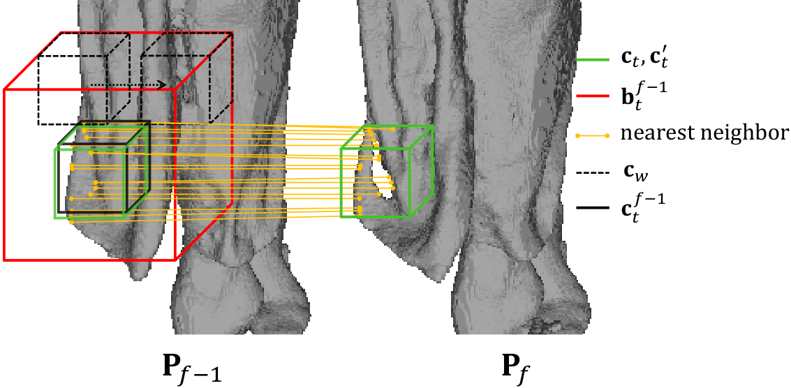
Considering that the inpainted results of dynamic point clouds should be coherent among consecutive frames, it is necessary to explore the temporal correspondence between neighboring frames in a point cloud sequence. Unlike videos, dynamic point clouds are irregular, thus the temporal correspondence is challenging to define.

In order to efficiently explore the temporal correspondence in dynamic point clouds for coherent inpainting, we propose to find corresponding cubes for $\mathbf{c}_{t}$ both in $\mathbf{P}_{f-1}$ and $\mathbf{P}_{f+1}$ , which are denoted by $\mathbf{c}_{t}^{f-1}$ and $\mathbf{c}_{t}^{f+1}$ respectively as the inter-source cubes. Note that, the inter-frame consistency can be generalized to several previous and subsequent frames, instead of one forward and one backward as in our method.

Specifically, inspired by the observation that a set of points representing the same region have little variation in consecutive frames, we find the temporal correspondence via searching the nearest neighbor of each point in the target cube. As shown in Fig. 3, we first find a co-located cube $\mathbf{c}^{\prime}_{t}\in\mathbb{R}^{M^{3}\times 3}$ in $\mathbf{P}_{f-1}$ as $\mathbf{s}(\mathbf{c}^{\prime}_{t})=\mathbf{s}(\mathbf{c}_{t})$ , where $\mathbf{s}(\cdot)$ denotes the coordinate of the centering point of a cube.

Then we construct a bounding box $\mathbf{b}_{t}^{f-1}\in\mathbb{R}^{H^{3}\times 3}$ ( $H$ is the size of the box) around $\mathbf{c}^{\prime}_{t}$ as $\mathbf{s}(\mathbf{b}_{t}^{f-1})=\mathbf{s}(\mathbf{c}^{\prime}_{t})$ , which serves as the search range. Next, we search the nearest neighbor in $\mathbf{b}_{t}^{f-1}$ of each point in $\mathbf{c}_{t}$ in terms of the relative location. Then we employ a sliding cubic window $\mathbf{c}_{w}\in\mathbb{R}^{M^{3}\times 3}$ with stride $1$ in the bounding box $\mathbf{b}_{t}^{f-1}$ to search for the inter-source cube $\mathbf{c}_{t}^{f-1}\in\mathbb{R}^{M^{3}\times 3}$ in $\mathbf{P}_{f-1}$ :

\mathbf{c}_{t}^{f-1}=\argmax_{\mathbf{c}_{w}}V(\mathbf{c}_{w}),\vskip-9.39545pt

(2)

where $V(\mathbf{c}_{w})$ is the number of the nearest neighbors of $\mathbf{c}_{t}$ in $\mathbf{c}_{w}$ in terms of the relative location. That is, $\mathbf{c}_{t}^{f-1}$ contains the most nearest neighbors of points in $\mathbf{c}_{t}$ .

We further perform the same structure matching on $\mathbf{c}_{t}^{f-1}$ as the way we deal with $\mathbf{c}_{s}$ in Section 3.1, which leads to the final inter-source cube in $\mathbf{P}_{f-1}$ , denoted as $\hat{\mathbf{c}}_{t}^{f-1}$ . The final inter-source cube in $\mathbf{P}_{f+1}$ , denoted by $\hat{\mathbf{c}}_{t}^{f+1}$ , is searched in the same way as in $\mathbf{P}_{f-1}$ . Thus we obtain two source cubes as the temporal reference, which will be adopted in the final inpainting step.

3.3 Spatio-Temporal Graph Construction

To take advantage of both intra-frame self-similarity and inter-frame consistency, we construct a spatial-temporal graph on the target cube $\mathbf{c}_{t}$ as the following.

We first build spatial connectivities within $\mathbf{c}_{t}$ . As there exists a hole in $\mathbf{c}_{t}$ , we approximate the connectivities via the similarities in its intra-source cube $\hat{\mathbf{c}}_{s}$ . We choose to build a $K$ -NN graph mentioned in Section 2, based on the affinity of geometric distance among points in $\hat{\mathbf{c}}_{s}$ . Specifically, the edge weight $w_{k,l}$ between nodes $k$ and $l$ in $\hat{\mathbf{c}}_{s}$ is assigned as

w_{k,l}=\begin{cases}~\text{exp}\{-\frac{\lVert\mathbf{p}_{k}-\mathbf{p}_{l}\rVert_{2}^{2}}{2\sigma^{2}}\},&k\sim l\\ ~0,&\text{otherwise}\end{cases}\vskip-7.22743pt

(3)

where $k\sim l$ means nodes $k$ and $l$ are $K$ nearest neighbors and thus connected. $\sigma$ is a weighting parameter (empirically $\sigma=1$ in our experiments). This is based on the assumption that geometrically closer points are more similar in general.

We then construct temporal connectivities between $\mathbf{c}_{t}$ and its previous frame $\hat{\mathbf{c}}_{t}^{f-1}$ , as well as temporal connectivities between $\mathbf{c}_{t}$ and its subsequent frame $\hat{\mathbf{c}}_{t}^{f+1}$ . Due to the hole in $\mathbf{c}_{t}$ , the connectivities for known points and unknown points in $\mathbf{c}_{t}$ are linked in different manners. Specifically, we link each known point in $\mathbf{c}_{t}$ with its corresponding point in $\hat{\mathbf{c}}_{t}^{f-1}$ . To circumvent the unavailability of unknown points in $\mathbf{c}_{t}$ , we approximate the temporal connectivities by the similarities between their corresponding points in the intra-source cube $\hat{\mathbf{c}}_{s}$ and their corresponding points in the inter-source cube $\hat{\mathbf{c}}_{t}^{f-1}$ . The temporal correspondence is based on the the nearest neighbor in the relative location in the cube.

Further, we define a weight matrix $\mathbf{W}_{f-1}\in M^{3}\times M^{3}$ to encode the temporal connectivities between $\mathbf{c}_{t}$ and $\hat{\mathbf{c}}_{t}^{f-1}$ . The rows of $\mathbf{W}_{f-1}$ correspond to points in $\mathbf{c}_{t}$ and columns correspond to points in $\hat{\mathbf{c}}_{t}^{f-1}$ . Specifically, the weight in $\mathbf{W}_{f-1}$ between nodes $k$ and $l$ is assigned as

w_{k,l}=\begin{cases}~1,&k\sim l\\ ~0,&\text{otherwise}\end{cases}\vskip-7.22743pt

(4)

where $k\sim l$ means nodes $k$ and $l$ are temporally corresponding points and thus connected. We set weight $1$ to each pair of temporally connected points as the temporal correlation is strong for corresponding points.

It is the same for the construction of temporal connectivities between $\mathbf{c}_{t}$ and $\hat{\mathbf{c}}_{t}^{f+1}$ . Similarly, we define a weight matrix $\mathbf{W}_{f+1}$ to describe the temporal connections.

3.4 Problem Formulation

Finally, we cast dynamic point cloud inpainting as an optimization problem, which is regularized by the graph-signal smoothness prior as mentioned in Section 2 and temporal consistency. It is formulated as

\begin{split}\min_{\mathbf{c}_{r}}~~&\lVert\overline{\mathbf{\Omega}}\mathbf{c}_{r}-\overline{\mathbf{\Omega}}\mathbf{c}_{t}\rVert_{2}^{2}+\alpha\lVert\mathbf{\Omega}\mathbf{c}_{r}-\mathbf{\Omega}\hat{\mathbf{c}}_{s}\rVert_{2}^{2}+\gamma\mathbf{c}_{r}^{T}\mathcal{L}\mathbf{c}_{r}+\\ &\beta\lVert\mathbf{c}_{r}-\mathbf{W}_{f-1}\hat{\mathbf{c}}_{t}^{f-1}\rVert_{2}^{2}+\beta\lVert\mathbf{c}_{r}-\mathbf{W}_{f+1}\hat{\mathbf{c}}_{t}^{f+1}\rVert_{2}^{2}\end{split}\vskip-9.39545pt

(5)

where $\mathbf{c}_{r}\in\mathbb{R}^{M^{3}\times 3}$ is the desired resulting cube. $\mathbf{\Omega}$ is a $M^{3}\times M^{3}$ diagonal matrix with $\Omega_{i,i}\in\{0,1\}$ , where 0 indicates known points and 1 indicates missing points. Thus $\mathbf{\Omega}\mathbf{c}_{r}$ and $\mathbf{\Omega}\hat{\mathbf{c}}_{s}$ represent the missing region in $\mathbf{c}_{r}$ and $\hat{\mathbf{c}}_{s}$ respectively. $\overline{\mathbf{\Omega}}$ is complementary to $\mathbf{\Omega}$ , which extracts the known region. $\mathcal{L}$ is the Laplacian matrix of the spatial graph constructed over $\mathbf{c}_{t}$ as described in Section 3.3. $\alpha$ , $\beta$ and $\gamma$ are three weighting parameters (we empirically set $\alpha=1$ , $\beta=0.5$ and $\gamma=0.5$ in the experiments).

The first term in (5) is a data fidelity term, which ensures the desired cube to be close to $\mathbf{c}_{t}$ in the known region. The second term constraints the missing region of $\mathbf{c}_{r}$ to be similar to that of $\hat{\mathbf{c}}_{s}$ . The last two terms aim to make the structure of $\mathbf{c}_{r}$ mimic that of $\hat{\mathbf{c}}_{t}^{f-1}$ and $\hat{\mathbf{c}}_{t}^{f+1}$ , which enforces the temporal consistency. Further, the third term is the graph-signal smoothness prior, which enforces the internal structure of $\mathbf{c}_{r}$ to be smooth with respect to the constructed spatial graph when merging information from three source cubes.

(5) is a quadratic programming problem. Taking derivative of (5) with respect to $\mathbf{c}_{r}$ and setting the derivative to $0$ , we have the closed-form solution:

\begin{split}\mathbf{c}_{r}^{\text{opt}}=&(\overline{\mathbf{\Omega}}^{2}+\alpha\mathbf{\Omega}^{2}+2\beta\mathbf{I}+\gamma\mathcal{L})^{-1}\\ &(\overline{\mathbf{\Omega}}^{2}\mathbf{c}_{t}+\alpha\mathbf{\Omega}^{2}\hat{\mathbf{c}}_{s}+\beta\mathbf{W}_{f-1}\hat{\mathbf{c}}_{t}^{f-1}+\beta\mathbf{W}_{f+1}\hat{\mathbf{c}}_{t}^{f+1}).\end{split}

(6)

(5) is thus solved optimally and efficiently. We replace the target cube with the resulting cube in the target frame $\mathbf{P}_{f}$ , which serves as the output.

4 Experiments

4.1 Experimental Setup

We evaluate the proposed method by testing on several 3D dynamic point cloud datasets from MPEG [45] and JPEG Pleno [46], including Longdress, Loot, Redandblack, Soldier, and UlliWegner. We test on two types of holes: 1) real holes generated during the capturing process, which have no ground truth; 2) synthetic holes on point clouds so as to compare with the ground truth.

Further, we compare our method with three competing algorithms for static 3D geometry inpainting, including Meshlab [47], Lozes et al. [13] and Hu et al. [17]. We test the static methods by performing them on each frame separately. Besides, as Meshlab is based on meshes, we convert point clouds to meshes via the Meshlab software [47] prior to testing the method, and then convert the inpainted meshes back to point clouds as the final output.

4.2 Results on Point Cloud Inpainting

Objective results. It is nontrivial to measure the geometry difference of point clouds objectively. We apply the geometric distortion metrics in [48] and [8], referred to as GPSNR and NSHD, respectively, as the metric for evaluation. The higher GPSNR is and the lower NSHD is, the smaller the difference between two point clouds is.

Table 1 and Table 2 show the average objective results of the frames for each sequence with synthetic holes in GPSNR and NSHD, respectively. We see that our scheme outperforms all the competing methods in GPSNR and NSHD significantly. Specifically, in Table 1 we achieve 26.80 dB gain in GPSNR on average over Meshlab, 16.18 dB over [13] and 5.26 dB over [17]. In Table 2, we produce much lower NSHD than the other methods, at least three times lower compared to the next best method [17].

Table 1: Performance Comparison in GPSNR (dB)

	Meshlab[47]	Lozes[13]	Hu[17]	Proposed
Longdress	11.7926	30.3883	41.5686	43.1301
Loot	16.4451	27.3715	40.1546	47.5648
Redandblack	13.1772	24.4810	33.9921	39.0103
Soldier	17.4697	23.1571	34.5062	42.2980
UlliWegner	24.9424	31.5455	41.3037	45.8411

Table 2: Performance Comparison in NSHD (

\times 10^{-7}

)

	Meshlab[47]	Lozes[13]	Hu[17]	Proposed
Longdress	24.8631	7.1362	2.9174	0.9131
Loot	14.1925	8.9410	3.1102	0.3549
Redandblack	22.8300	9.6233	5.9856	1.9324
Soldier	17.1376	10.0044	5.2145	1.2057
UlliWegner	11.2509	6.7370	1.9658	0.6362

Subjective results. Further, Fig. 4 and Fig. 5 demonstrate the subjective inpainting results for real and synthetic holes, respectively. Due to the page limit, we show several representative frames compared with one competitive method [13]. For the real holes in Fig. 4 (a), which are fragmentary, the results of [13] exhibit artificial contours, since it attempts to connect the boundary of the hole region with planar structures without smoothing. However, the inpainted results are not smooth in the local region, which indicates the temporal inconsistency to some extent. In comparison, our results shown in row 3 of Fig. 4 demonstrate that our method is able to inpaint holes with appropriate geometry structure and smoothness over the hole region. Besides, since we leverage the inter-frame correlation, our inpainted regions show good consistency across neighboring frames.

In Fig. 5, we synthesize holes in the point cloud sequence Soldier, with more complex and bigger holes than the real holes in Fig. 4. We observe that [13] covers the missing area with stripy geometry, which introduces wrong geometry around the holes compared to the ground truth. Also, the contents look incoherent among the consecutive frames. In comparison, our results shown in row 3 of Fig. 5 are almost the same as the ground truth, and exhibit consistency between neighboring frames. This gives credits to the intra-frame self-similarity, the inter-frame consistency and graph-signal smoothness prior.

5 Conclusion

We propose a novel 3D dynamic point cloud inpainting method. The key idea is to enforce both intra-frame self-similarity and inter-frame consistency in point cloud sequences. Given a target cube with holes inside, we propose to efficiently search for its intra-frame self-similar cube and inter-frame corresponding cubes. We then cast dynamic point cloud inpainting as a quadratic programming problem, based on the searched source cubes and regularized by the graph-signal smoothness prior. Experimental results show that our algorithm significantly outperforms three competing methods. Future works include the extension to inpainting the attributes of dynamic point clouds.

References

[1] C. Loop, C. Zhang, and Z. Zhang, “Real-time high-resolution sparse voxelization with application to image-based modeling,” in High-performance Graphics Conference, 2013.
[2] C. Tulvan, R. Mekuria, and Z. Li, “Use cases for point cloud compression (pcc),” in ISO/IEC JTC1/SC29/WG11 (MPEG) output document N16331, June 2016.
[3] P. Chalmoviansky and B. Juttler, “Filling holes in point clouds,” in Mathematics of Surfaces. Springer Berlin Heidelberg, 2003, pp. 196–212.
[4] P. Sahay and A. N. Rajagopalan, “Harnessing self-similarity for reconstruction of large missing regions in 3D models,” in International Conference on Pattern Recognition, 2012, pp. 101–104.
[5] ——, “Geometric inpainting of 3D structures,” in Computer Vision and Pattern Recognition Workshops, 2015, pp. 1–7.
[6] S. Shankar, S. A. Ganihar, and U. Mudenagudi, “Framework for 3D object hole filling,” in Fifth National Conference on Computer Vision, Pattern Recognition, Image Processing and Graphics, 2015, pp. 1–4.
[7] S. Shankar and U. Mudenagudi, “Example-based 3d inpainting of point clouds using metric tensor and christoffel symbols,” Machine Vision and Applications, vol. 29, pp. 329–343, 2018.
[8] C. Dinesh, I. V. Bajic, and G. Cheung, “Exemplar-based framework for 3D point cloud hole filling,” in IEEE International Conference on Visual Communications and Image Processing, May 2017.
[9] ——, “Adaptive non-rigid inpainting of 3d point cloud geometry,” IEEE Signal Processing Letters, vol. 25, no. 6, pp. 878–882, 2018.
[10] J. Wang, M. M. Oliveira, M. Garr, and M. Levoy, “Filling holes on locally smooth surfaces reconstructed from point clouds,” Image & Vision Computing, vol. 25, no. 1, pp. 103–113, 2007.
[11] Y. Quinsat and C. Lartigue, “Filling holes in digitized point cloud using a morphing-based approach to preserve volume characteristics,” International Journal of Advanced Manufacturing Technology, vol. 81, no. 1-4, pp. 411–421, 2015.
[12] F. Lozes, A. Elmoataz, and O. Lézoray, “Partial difference operators on weighted graphs for image processing on surfaces and point clouds,” IEEE Transactions on Image Processing, vol. 23, no. 9, pp. 3896–909, 2014.
[13] ——, “PDE-based graph signal processing for 3-D color point clouds : opportunities for cultural heritage,” IEEE Signal Processing Magazine, vol. 32, no. 4, pp. 103–111, 2015.
[14] H. Lin and W. Wang, “Feature preserving holes filling of scattered point cloud based on tensor voting,” in IEEE International Conference on Signal and Image Processing, 2017, pp. 402–406.
[15] Y. Muraki, K. Nishio, and T. Kanaya, “An automatic hole filling method of point cloud for 3d scanning,” 2017.
[16] Z. Fu, W. Hu, and Z. Guo, “Point cloud inpainting on graphs from non-local self-similarity,” in IEEE International Conference on Image Processing, Athens, Greece, 2018.
[17] ——, “Local frequency interpretation and non-local self-similarity on graph for point cloud inpainting,” arXiv:1810.03973v1, 2018.
[18] D. I. Shuman, S. K. Narang, P. Frossard, A. Ortega, and P. Vandergheynst, “The emerging field of signal processing on graphs: Extending high-dimensional data analysis to networks and other irregular domains,” IEEE Signal Processing Magazine, vol. 30, no. 3, pp. 83–98, 2013.
[19] A. Ortega, P. Frossard, J. Kovačević, J. M. F. Moura, and P. Vandergheynst, “Graph signal processing,” IEEE Journal of Selected Topics in Signal Processing, vol. 11, no. 6, pp. 771–773, 2017.
[20] P. Berger, G. Hannak, and G. Matz, “Graph signal recovery via primal-dual algorithms for total variation minimization,” IEEE Journal of Selected Topics in Signal Processing, vol. PP, no. 99, pp. 1–1, 2017.
[21] Y. Bai, G. Cheung, X. Liu, and W. Gao, “Blind image deblurring via reweighted graph total variation,” in IEEE International Conference on Acoustics, Speech and Signal Processing, Calgary, Alberta, Canada, 2017.
[22] X. Liu, G. Cheung, X. Wu, and D. Zhao, “Inter-block consistent soft decoding of jpeg images with sparsity and graph-signal smoothness priors,” in IEEE International Conference on Image Processing, 2015, pp. 1628–1632.
[23] X. Dong, D. Thanou, P. Frossard, and P. Vandergheynst, “Over- and under-exposure reconstruction of a single plenoptic capture,” IEEE Transactions on Signal Processing, vol. 64, no. 23, pp. 6160–6173, Dec. 2016.
[24] W. Hu, M. Seifi, and E. Reinhard, “Over- and under-exposure reconstruction of a single plenoptic capture,” ACM Transaction on Multimedia Computer Communication Application, vol. 14, no. 2, pp. 52:1–52:21, May 2018.
[25] S. Friedman and I. Stamos, “Online facade reconstruction from dominant frequencies in structured point clouds,” in Computer Vision and Pattern Recognition Workshops, 2012, pp. 1–8.
[26] X. Wu and W. Chen, “A scattered point set hole-filling method based on boundary extension and convergence,” in Intelligent Control and Automation, 2015, pp. 5329–5334.
[27] C. Chen and B. Yang, “Dynamic occlusion detection and inpainting of in situ captured terrestrial laser scanning point clouds sequence,” Isprs Journal of Photogrammetry & Remote Sensing, vol. 119, pp. 90–107, 2016.
[28] F. K. Chung, “Spectral graph theory,” vol. 92, no. 6, p. 212, 1996.
[29] A. Sandryhaila and J. M. F. Moura, “Discrete signal processing on graphs,” IEEE Transactions on Signal Processing, vol. 61, no. 7, pp. 1644–1656, 2013.
[30] G. Shen, W.-S. Kim, S. K. Narang, A. Ortega, J. Lee, and H. Wey, “Edge-adaptive transforms for efficient depth map coding,” in IEEE Picture Coding Symposium, Nagoya, Japan, December 2010, pp. 566–569.
[31] W. Hu, G. Cheung, X. Li, and O. C. Au, “Depth map compression using multi-resolution graph-based transform for depth-image-based rendering,” in IEEE International Conference on Image Processing, Orlando, FL, September 2012, pp. 1297–1300.
[32] W. Hu, G. Cheung, A. Ortega, and O. C. Au, “Multi-resolution graph fourier transform for compression of piecewise smooth images,” in IEEE Transactions on Image Processing, vol. 24, no. 1, January 2015, pp. 419–33.
[33] D. A. Spielman, “Lecture 2 of spectral graph theory and its applications,” September 2004.
[34] X. Liu, G. Cheung, X. Wu, and D. Zhao, “Random walk graph laplacian-based smoothness prior for soft decoding of JPEG images,” IEEE Transactions on Image Processing, vol. 26, no. 2, pp. 509–524, Feb. 2017.
[35] X. Liu, G. Cheung, C. Lin, D. Zhao, and W. Gao, “Prior-based quantization bin matching for cloud storage of jpeg images,” IEEE Transactions on Image Processing, vol. 27, no. 7, pp. 3222–3235, July 2018.
[36] X. Liu, G. Cheung, X. Ji, D. Zhao, and W. Gao, “Graph-based joint dequantization and contrast enhancement of poorly lit jpeg images,” IEEE Transactions on Image Processing, pp. 1–1, 2019.
[37] A. V. Oppenheim, R. W. Schafer, , and J. R. Buck, “Discrete-time signal processing,” 1989.
[38] M. Puschel and J. M. F. Moura, “Algebraic signal processing theory: Foundation and 1-d time,” IEEE Transactions on Signal Processing, vol. 56, no. 8, pp. 3572–3585, 2008.
[39] ——, “Algebraic signal processing theory: 1-d space,” IEEE Transactions on Signal Processing, vol. 56, no. 8, pp. 3586–3599, 2008.
[40] P. J. Besl and N. D. Mckay, “A method for registration of 3-D shapes,” IEEE Transactions on Pattern Analysis & Machine Intelligence, vol. 14, no. 2, pp. 239–256, 2002.
[41] D. Chetverikov, D. Svirko, D. Stepanov, and P. Krsek, “The trimmed iterative closest point algorithm,” in International Conference on Pattern Recognition, 2002. Proceedings, vol. 3, 2002, pp. 545–548.
[42] K. Julius, B. Nico, R. R. Bogdan, B. Michael, S. Eckehard, and G. Suat, “Real-time compression of point cloud streams,” in IEEE International Conference on Robotics & Automation, 2012.
[43] D. Thanou, P. A. Chou, and P. Frossard, “Graph-based compression of dynamic 3d point cloud sequences,” IEEE Transactions on Image Processing, vol. 25, no. 4, pp. 1765–1778, 2016.
[44] T. Biyikogu, J. Leydold, and P. F. Stadler, “Laplacian eigenvectors of graphs,” Lecture Notes in Mathematics, vol. 1915, 2007.
[45] T. Ebner, I. Feldmann, O. Schreer, P. Kauff, and T. Unger, “Hhi point cloud dataset of a boxing trainer,” in ISO/IEC JTC1/SC29/WG11 (MPEG2018) input document M42921, July 2018.
[46] E. d’Eon, B. Harrison, T. Myers, and P. A. Chou, “8i voxelized full bodies, version 2 - a voxelized point cloud dataset,” in ISO/IEC JTC1/SC29/WG11 (MPEG2017) input document M40059, January 2017.
[47] P. Cignoni, M. Callieri, M. Corsini, M. Dellepiane, F. Ganovelli, and G. Ranzuglia, “Meshlab: an open-source mesh processing tool,” in Eurographics Italian Chapter Conference, S. Vittorio, D. C. Rosario, and F. Ugo, Eds. The Eurographics Association, 2008.
[48] D. Tian, H. Ochimizu, C. Feng, R. Cohen, and A. Vetro, “Geometric distortion metrics for point cloud compression,” in IEEE International Conference on Image Processing, Beijing, China, September 2017.