Exponentially Decaying Extended Emissions Following Short Gamma-Ray Bursts with Possible Luminosity – E-folding Time Correlation Journal: ApJXSPEC (Arnaud 1996, v12.10.0)
Abstract
The origin of extended emissions following prompt emissions of short gamma-ray bursts (SGRBs) is in mystery. The long-term activity of the extended emission is responsible for promising electromagnetic counterparts to gravitational waves and, so that it may be a key to uncovering the progenitor of SGRBs. We investigate the early X-ray light curves of 26 SGRBs with known redshifts observed with the X-Ray Telescope aboard the Neil Gehrels Swift Observatory (Swift). We find that the exponential temporal decay model is able to describe the extended emissions comprehensively with a rest-frame e-folding time of 20 – 200 seconds. We also estimate the isotropic equivalent energies of the extended emission with the exponential decay model and of the prompt emission, compared with those of the prompt emission. Then, it is revealed that the extended emission is 0 – 3 orders of magnitude less powerful than the prompt emission. We find a strong correlation between the expected maximum luminosity and e-folding time which can be described by a power-law with an index of and whose chance probability of if there is no observation bias of Swift. The exponential temporal decay may be interpreted to come from the spin-down time scale of the rotation energy of a highly magnetized neutron star, and/or fallback accretion onto a disk surrounding a black hole with an exponentially decaying magnetic flux by magnetic reconnection.
Keywords:
gamma-ray burst:general - stars:black holes -I Introduction
Short gamma-ray bursts (SGRBs) are a sub-class of gamma-ray bursts (GRBs) with a duration of less than about 2 seconds. Some SGRBs are followed by temporally extended soft X-ray emission lasting about 100 seconds (Norris & Bonnell 2006). In addition, most of the extended emissions were also reported to have comparable energy fluences with the prompt emissions (Perley et al. 2009; Bostanci et al. 2012).
SGRBs are thought to originate from a coalescence of binary compact objects such as neutron star – neutron star and/or black hole – neutron star (Paczynski 1986; Eichler et al. 1989). In this scenario, a relativistic jet is launched from the remnant and then powers the prompt emission. Additionally, the merger is also expected to emit strong gravitational waves (GWs). In fact, GW170817 observed by the LIGO-Virgo collaboration originated from a binary neutron star merger (Abbott et al. 2017). Therefore SGRBs and the following extended emissions are promising electromagnetic counterparts to GW events. In particular, the extended emission may be more isotropic than the beamed prompt emission because of a weak variability of the observed light curve (Bucciantini et al. 2012, opening angle of ;). SGRB afterglows following the extended emission would be also important for the localization of GW sources. In general, the afterglow can be distinguished by two or more segments such as a shallow-decay emission, so-called plateau emission with a duration of – seconds, (Gompertz et al. 2013; Gompertz et al. 2014), and a normal-decay component, which is thought to arise from an external shock between the relativistic jet and the circumburst medium swept up by the jet (Paczynski 1993; Gehrels et al. 2005, e.g.,).
The origin of the temporally extended emission is, however, still in mystery. This has been also debated for some cases of the merger remnant, for example, a spin-down energy loss of a rapidly spinning magnetar (Metzger et al. 2008) and/or a fallback accretion of tidally ejected mass onto a disk surrounding a black hole (Barkov & Pozanenko 2011; Kisaka & Ioka 2015). The type of the remnant depends on the equation of state of the neutron star and the total binary mass.
In order to reveal the origin of the extended emission, some studies on the temporal behavior were performed (Gompertz et al. 2014; Nathanail et al. 2015, e.g.,). From the magnetar engine model, the X-ray light curves of SGRBs can be described by the power-law decay index of by considering the dipole radiation (Zhang & Mészáros 2001, e.g.,). The study of the light curves following SGRBs with this decay slope have been performed (Lü et al. 2015, e.g.,). Kisaka et al. 2017 discussed a power-law model with a power-law index of (Kisaka & Ioka 2015) by considering the black hole engine model with Blandford – Znajek jet (Blandford & Znajek 1977) and ejecta fallback (Rosswog 2007, e.g.,), and then from the observed light curve study with this model, it was concluded that in the luminosity – duration plane the extended emission has a different distribution from that of the plateau emission (i.e., bimodal distribution).
On the other hand, Kagawa et al. 2015 reported that the exponential temporal decay model was able to fit some extended emissions with an e-folding time of 50 – 100 seconds. Similar studies on the exponential decay has been performed for early X-ray emissions of long GRBs (LGRBs) (Willingale et al. 2007; Sakamoto et al. 2007; Imatani et al. 2016, e.g.,). Therefore, in this paper, we report a systematic study on phenomenological modeling for the extended emission light curves of SGRBs by adopting the exponential and power-law decay models, and a comparison of both models for discussing which model is suitable for describing the observed light curves of the extended mission.
This paper is constructed as follows. In Section II, we create X-ray light curves of the extended emission following 26 SGRBs with known redshifts. In Section III, we systematically study the temporal decay properties of the extended emission by adopting two types models; exponential and phenomenological power-law decay models. Then, in Section IV, comparing these models, we confirm that the exponential decay model comprehensively describes most of the extended emissions. After that, we precisely compare the bolometric energy of the prompt emission with that of the extended emission integrated over the entire exponential decay model. Then, we find a strong correlation between the expected maximum luminosity and the e-folding time of the exponential model. Finally, we discuss physical origins of the extended emission represented by the exponential decay model.
II Spectral analysis
II.1 Event Selection
First, we pick up 114 SGRBs with a duration of seconds from the Neil Gehrels Swift Observatory (Swift) GRB webpage11 1 https://swift.gsfc.nasa.gov/, detected until the end of August 2018, where corresponds to the time interval which contains the 90% of the total observed photons in the 50 – 300 keV energy band. We also focus on possible SGRB candidates whose is longer than 2 seconds due to the bright extended emission episode following the prompt initial spikes. From the events reported in the GRB Coordinates Network (GCN) circulars22 2 https://gcn.gsfc.nasa.gov/, we include 14 possible SGRBs whose of initial spike is less than 2 seconds33 3 GRB 050911, 061210 080123, 080503, 090531B, 090715A, 090916, 091117, 100213A, 110402A, 130716A, 130822A, 150424A, and 160303A. In addition, we add 13 GRBs whose of the initial spike is slightly larger than 2 seconds but considered to be SGRB events because their spectral time lags are consistent with zero which is expected in general SGRBs44 4 GRB 051227, 060717, 100816A, 161001A, 160303A, 171103A, and 180618A (Cheng et al. 1995; Yi et al. 2006, e.g.,), or they have a hard spectral photon index55 5 050724, 060614, 061006, 070714B, 090309, and 171007A (Kouveliotou et al. 1993, e.g.,). Next, we select SGRBs with known redshifts from the event list to correct the observed flux to the isotropic luminosity in order to investigate the intrinsic behavior.
We use the X-ray extended, plateau, and/or normal-decay emissions data observed by the Burst Alert Telescope (BAT) and the X-Ray Telescope (XRT) (Gehrels et al. 2004) to investigate the early X-ray properties of SGRBs. Some extended emissions were not observed with the BAT but with only the XRT (Kagawa et al. 2015; Kisaka et al. 2017). Thus, in order to discuss the extended emissions comprehensively, it is necessary to analyze the X-ray data of SGRBs. Since extended emissions are thought to last seconds, we exclude 4 events observed by the XRT over 300 seconds since the triggers66 6 GRB 061210, 071010B, 150101B, and 170428A. Furthermore, we refer UK Swift Science Data Center77 7 http://www.swift.ac.uk/index.php, 88 8 http://www.swift.ac.uk/xrt_curves which shows the quick look data of observed SGRBs obtained by the automatic analysis (Evans et al. 2007; Evans et al. 2009). We also reject 7 dim bursts99 9 GRB 060502B, 061217, 070429B, 071112, 100206A, 140622A, and 141212A whose X-ray light curves of the XRT data consist of 4 or less data points because a light curve fitting model described in Section III has 5 free parameters. After these event selections, we obtain 26 SGRBs with known redshifts as listed in Table 13 from the 141 Swift SGRBs (including SGRB candidates).
II.2 Light Curve Creation based on Spectral Analysis for the XRT Data
First, we extract X-ray signals within an image region of rectangular pixels with a rotation angle along the spacecraft attitude for windowed timing (WT) mode data, and 20 pixels in radius (corresponding to 47 arcsec) for photon counting (PC) mode data. These are recommended region sizes described in the Swift/XRT software guide version 1.21010 10 https://swift.gsfc.nasa.gov/analysis/. We also extract a background signal from the image region without any X-ray sources (under the sensitivity of the XRT). The region size is a rectangular with pixels for WT mode, and a circle as large as possible (at least 20 pixels) for PC mode data. The source and background regions do not overlap with each other.
After that, we perform time-resolved spectral analysis and estimate precise energy flux of the extended emission. This is because the extended emission generally shows rapid spectral softening (Kagawa et al. 2015), and a common method of conversion from photon flux to energy flux with average spectral parameters can not be adopted for the extended emission. Then we extract time-resolved spectra from WT and PC mode data of the selected SGRBs. In order to conserve an uniform statistical uncertainty for each spectrum, we divide the entire data into several time bins to keep the same number of photons (about 256 photons for WT mode, and 128 photons for PC mode, respectively) inside each time bin.
We consider a single power-law spectral model considering Galactic and extra-galactic photo-electric absorptions (“phabs” and “zphabs” model, respectively). The exact formula of the model is
| (1) |
Here, is in units of . and are the Galactic and extra-galactic hydrogen column density, in units of , respectively. is a photo-electric cross-section (not including Thomson scattering) and is a redshift. A quantity is a normalization of power-law model of 1 keV and is a photon index. We perform spectral fitting with this model for the time-resolved spectra using XSPEC version 12.10.0 (Arnaud 1996), and obtain the best-fit parameters. the results are shown in Figure 1. The photon absorption below keV may affect the flux estimate. Thus, to suppress the uncertainty of the absorption we adopt an energy band of 2/ – 10/ keV corresponding to the 2 – 10 keV band in the rest frame.
Additionally, we perform a time-averaged spectral analysis for the PC mode data to investigate the light curve of dim events in the selected SGRBs. First, we make a light curve of photon count rate in which each time bin contains 25 photons at least to keep the statistical uncertainty. Then, we make an integrated spectrum during the same epoch of the created light curve. We can obtain the time-averaged energy flux and spectral parameters, and also estimate a conversion factor from the average photon flux to the averaged energy flux. After that, we create the light curve in energy flux with the conversion factor on the assumption that the spectral parameters are stable during the focusing epoch. The obtained the light curve of the energy flux with time-averaged spectral analysis are also shown in Figure 1. In this work, for the PC mode data, we adopt the time-averaged spectral analysis.
II.3 Swift/BAT Detection
Since the extended emission in GRB 050724, 060614, and 070714B are bright, and detected with the BAT, we are able to perform a single power-law fit for the energy spectra of the Swift/BAT data. We show the fitting results of the energy flux and photon index in Figure 1. Here, for the BAT data, the energy flux is extrapolated to 2/ – 10/ keV band from the data of 15 – 150 keV in the observer frame.
For the other bursts without significant detection by the BAT, we give a detection limit of the BAT. Extrapolating the 5 sensitivity curve of erg cm-2 s-1 (in 15 – 150 keV) (Lien et al. 2016), we provide the limit in the energy band of 2/ – 10/ keV. Here, is a integration time in the observer frame since the burst trigger in units of second, and we assume that the photon index of the energy spectrum is 2, which is an averaged value of the three events detected with the BAT as shown in Figure 1 and consistent with the results of previous works (Kaneko et al. 2015; Lien et al. 2016, e.g.,). This sensitivity curve is adopted in the fitting analysis of the light curves (Section III.2) and the discussion about the suitable model for the extended emission light curve (Section IV.1).
III Light Curve Modeling
III.1 Exponential and Power-law Decay Models
In Kisaka et al. 2017, the extended emissions were systematically investigated with a phenomenological power-law decay model. An exponential decay model was reported to be also acceptable to describe some extended emissions in Kagawa et al. 2015. In this paper, we study the X-ray light curves of the selected SGRBs for the extended emission components with two models: the exponential (EXP) model and phenomenological power-law (PL) model. Both models contain the phenomenological power-law decay component to describe the following plateau and/or normal-decay emission episodes (Kisaka & Ioka 2015). The exact light curve models are as follows;
| (2) |
for the EXP model, and
| (3) |
for the PL model, respectively. Here, is a rest-frame time since the burst trigger, and an isotropic luminosity is in units of erg s-1. Parameters , , and are the normalization of isotropic luminosity and the rest-frame durations of the extended and plateau emissions since the burst trigger, respectively. Parameters and are temporal indices of the extended and plateau emissions, respectively. In EXP model, is an e-folding time in the rest frame of SGRBs. These two functions are referred from Yamazaki 2009; Kagawa et al. 2015; Kisaka & Ioka 2015; Kisaka et al. 2017.
In this work, we systematically perform temporal fitting with both EXP and PL models, and compare the fitting results. Here, we consider three cases, (I) EXP model with the free parameter , (II) PL(BH) model with the fixed parameters , and as 40/9 4.44, and an additional case of (III) PL(MG) model with the fixed parameters and as 2. The value of 40/9 in case (II) is derived in Kisaka & Ioka 2015 by considering the black hole engine model with Blandford - Znajek jet (Blandford & Znajek 1977) and ejecta fallback (Rosswog 2007, e.g.,). Case (III) corresponds to the dipole spin-down formula usually considered in magnetar model (Zhang & Mészáros 2001, e.g.,). Note that we discuss only the extended emission component in this paper.
III.2 Fitting Results
In Figure 2, we show X-ray light curves in terms of isotropic luminosity of the selected SGRBs estimated in Section II.2 and II.3 and also the best-fitted model functions. Here, to convert energy flux to isotropic luminosity, we use cosmological parameters of Hubble constant km s-1 Mpc-1, matter density , and dark energy density (Aghanim et al. 2018).
First, we evaluate whether the flux expected from the EXP model is consistent with the BAT detection limit described in Section II.3. For GRB 090510 and 100816A, due to poor statistics at the early observation phase, we could not constrain the fitting parameters such as and . Therefore, for these events, we set the maximum value of as an upper limit when we assume the EXP model does not exceed the BAT detection limit curve. For GRB 080123 and 150424A, there were bright X-ray sources in the field of view of the BAT and/or unexpected background fluctuations were observed as reported in Lien et al. 2016. Thus, we allow these GRBs to be included in this analysis as an exceptional case that the best-fit EXP curve of these events exceed the BAT detection limit. This is further described in Section II.3.
We summarize the best-fit parameters of light curve fitting in Table 2. In this table, the results of plateau emission components are not given because the parameters for most SGRBs are not precisely determined. In Section IV.1, we discuss which model is suitable for explaining the extended emission.
III.3 Estimate of Isotropic Equivalent Energy
Kisaka et al. 2017 showed a comparison of the isotropic energies of the prompt and the temporally extended emissions. In some works, the fluences of these emission were also compared, where both emissions data are observed with only the BAT (Perley et al. 2009; Bostanci et al. 2012). On the other hand, the energy spectra of GRBs are generally well described by a power-law function with exponential bending, so-called the Band function (Band et al. 1993), or a power-law function with exponential cutoff (Sakamoto et al. 2005, e.g.,). In the spectrum, the bending energy, called peak energy , is the most intense and typically in 200 – 300 keV (Kaneko et al. 2006). Therefore, for the energy band of the Swift/BAT (15 – 150 keV), it is too narrow to measure the bolometric energy of the prompt emission, and the previous works may underestimate the isotropic energy of the prompt emissions as described in Kisaka et al. 2017.
In order to estimate the precise bolometric energy of the prompt emission, we use the data of 15 events coincidently detected with the Swift/BAT and other detectors with wide energy range, WIND/Konus (Aptekar et al. 1995), Suzaku/Wide-band All-sky Monitor (WAM) (Yamaoka et al. 2005), and/or Fermi/Gamma-ray Burst Monitor (GBM) (Meegan et al. 2009). The isotropic equivalent energy of the prompt emission, , is calculated from the fluence of SGRBs which consists of only the initial spike component as reported in the GCN circular. We show the events and their prompt energies in Table 17.
In the case of the extended emission components, the estimate of the isotropic energy depends on the light curve model. The most extended emissions are not observed in the BAT energy range, and their energy spectra have not been measured. Thus, we compare the bolometric prompt emission energy with the one of the extended emission in 2 – 10 keV. For the EXP and PL models, the isotropic equivalent energy in the rest frame energy band of 2 – 10 keV is provided with
| (4) |
and (Kisaka et al. 2017), respectively. In Section IV.2, we show the comparison of the isotropic energies of the prompt and extended emissions.
IV Discussion
We systematically analyzed the early X-ray decay properties of the selected SGRBs with known redshifts observed by the Swift satellite. In this section, we discuss the suitable model for the temporally extended emission and its physical origin.
IV.1 Comparison of the Temporal Decay Models
As shown in Figure 2, the EXP model curve looks consistent with the observed light curve of all the selected SGRBs. In particular, for the three brightest events in the XRT energy band (GRB 050724, 060614, and 160821B), the EXP model is better than the PL(BH) model whose decay slope of is not steep enough to follow the rapid decay of the extended emissions. We note that for GRB 050724, the PL(BH) model is also acceptable because the data points near 1000 s is well followed. However, as shown in Figure 1 in Campana et al. 2006, a flaring activity was clearly detected at 1000 s, and the data hump is not the extended emission component. Therefore we conclud the EXP model which clearly follows the rapid decay light curve and is better than the PL(BH) model.
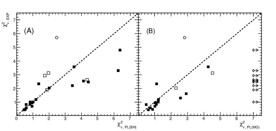
Then, to systematically compare the EXP and PL(BH) models, we show a scatter plot on the reduced of these models ( plane) in Figure 3 (A). For events with , both the models can be almost equally accepted because of . However, for events with , the EXP model is favored because of for most events. For the four events with , although at first glance these events favor the PL(BH) model, two of the four events (GRB 070724 and 100117A) apparently reject the PL(BH) model because the light curves extrapolated earlier violate the the BAT detection limit (see Figure 2). In addition, for one of the four events, GRB 160624A, the obtained best-fitted curve of both the models is not statistically significant because of less number of the flux points (e.g., the degrees of freedom of the fitting results for the EXP and PL(BH) models are only 1 and 2, respectively, as listed in Table 2). Eventually, we find that only a event (GRB 051221A) significantly favors the PL(BH) model. Thus, we conclude that in order to explain the extended emission light curve comprehensively, the EXP model is favored.
We also show the results of PL(MG) model fitting in Figure 2 and the best fit parameters are listed in Table 2, where we use events whose reduced of the PL(MG) model () is smaller than 7. Here, we do not discuss the PL(MG) model for GRB 061201 and 130603B because in PL(MG) model are not determined well, although the reduced shows that this model is acceptable. Then, we show the scatter plot on plane in Figure 3 (B). The observed extended emission systematically prefers the EXP model over the PL(MG) model, although only one event, GRB 051221A, clearly favors the PL(MG) model. Note that as is the case with the PL(BH) model, for five events such as GRB 090510, 100816A, 160624A, the best-fit model curves exceed the BAT detection limit and the PL(MG) model is fully rejected for the five events.
After all, we argue that for the EXP model, it is reasonable to describe the early X-ray light curve of 23 of the 24 selected SGRBs, where GRB 090510 and 100816A are not included. As shown in Table 2, the e-folding times of the temporal decay are 20 – 200 seconds and the in the rest-frame energy band of 2 – 10 keV is less than erg s-1. For both the PL(BH) and PL(MG) models, it is hard to explain the observed light curve of the extended emission comprehensively.
IV.2 Comparison with Prompt Emissions
We show the equivalent isotropic energies of the prompt and the extended emissions in Figure 4 and Table 17, considering that the extended emissions are described by the EXP model. Both isotropic energies are estimated in Section III.3. As shown in Figure 4, the extended emission has energies smaller by a factor of 0.001 – 1 than those of the prompt emission. Previous works showed that the time-averaged flux of the extended emissions is brighter than that of the prompt emission (Perley et al. 2009; Bostanci et al. 2012), and the isotropic energies of these emissions are roughly comparable (Kisaka et al. 2017). Thus the obtained result in this paper is different from that of the previous studies. This is because we include dim GRB events detected only with the XRT that were not included for the previous works and use more precise values of the than those in previous works.
In this paper, we use the extended emission data in the 2 – 10 keV energy band in the rest frame as described in Section II.2, which is different from that of the previous work (Kisaka et al. 2017, 0.3 – 10 keV;). Note that for events with (GRB 111117A and 160410A), the energy flux and also isotropic energy may have an uncertainty due to the unabsorbed power-law spectrum analysis avoiding the photon absorption below 1 keV in the observer frame. Then, we consider an under estimate of the isotropic energy of the extended emission caused by difference between 2 – 10 keV and 0.3 – 10 keV. In Figure 5, we show a histogram of the photon index obtained by performing the time-resolved analysis for the WT mode data, where we assume that the WT mode observed only the extended emission component. The photon indices of the extended emission are typically , and Figure 1 (e.g., GRB 050724, 060614, 150424A) shows the decay phase with are almost in dimmer phase of the decaying extended emission which hardly contributes to the energy estimate. The ratio of these fluxes in 2 – 10 keV to 0.3 – 10 keV with the photon index of 1 – 2 is at least , and so that the underestimate hardly affects our conclusion. Note that the XRT can hardly observe the early flat phase of the extended emission and the extended emission has spectral softening from to 2 or more during seconds (Kagawa et al. 2015). Thus the histogram of the obtained photon index of the extended emission may be biased to soften.
If we consider the case that the energy spectrum of the extended emission has the peak energy of keV, its bolometric energy should be modified. The photon index in 2 – 10 keV at the observed early phase is as shown in Figure 1 (e.g., GRB 050724, 060614, 070714B), and the one of the BAT spectrum before the XRT observations is (see Section II.3). Thus, the peak energy of the extended emission before its decaying phase is thought to be around the lower threshold of the BAT energy range of keV. Assuming the spectral shape of a broken power-law with the break energy of 15 keV and low/high-energy photon indices of 1 and 2, respectively, we estimate that the energy fluxes in 2 – 150 keV is larger by a factor of than that in 2 -- 10 keV1111 11 The ratio of the energy fluxes in 2 – 150 keV to 2 – 10 keV is .. In such case, the ratio of becomes closer to unity compared with the one of 2 – 10 keV as shown in Figure 4. We conclude that the majority of the extended emissions have the isotropic energy comparable to or slightly less than that of the prompt emissions.
IV.3 Correlation
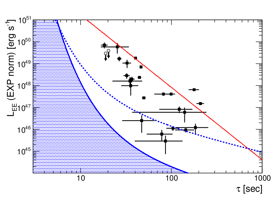
Assuming that all of the selected SGRBs are followed by the exponential decay, we show a scatter plot on - plane (listed in Table 2) in Figure 6. There is a strong negative correlation between and with the Spearman’s rank order correlation coefficient of and chance probability of . By performing a power-law fit for the data, we obtain
| (5) |
where is normalized at seconds which is an observed shortest value in the fitting results as listed in Table 2.
Figure 6 shows lack of events on the upper-right (long and bright) and lower-left (short and dim) areas. Such deserts could be caused by observation bias which makes the apparent correlation. Thus, we carefully consider the observation bias of the Swift/XRT observation. First, in the case of the long and bright events, if there existed such events, the events should have been confidently detected. However, no detection of such events indicates that intrinsically there is no long and bright event. Next, in the case of the short and dim events, such events might belong to sub- or under-threshold events observed with the XRT and we detailedly consider the XRT sensitivity of observation for the extended emission.
We consider that the XRT starts to observe a burst with a sensitivity, erg cm-2 s-1 (in 0.3 – 10 keV) (Burrows et al. 2005), at second in the observer frame after a burst trigger, where is an integration time after the XRT starts an observation. The energy sensitivity of the XRT in a rest-frame energy band of keV and a rest-frame duration is described as [erg], where,
| (6) |
and is a luminosity distance in unit of cm. Since the extended emission at early phase has a hard energy spectrum as shown in Figure 1 (e.g., GRB 050724, 060614, 070714B), we make an assumption that the photon index for the power-law spectrum of equals to 1. When, seconds after a burst, the XRT observes the extended emission for seconds, the following relation should be satisfied for the XRT to detect the extended emission,
| (7) |
Therefore, the observational luminosity limit of the XRT, , as a function of an e-folding time with a parameter is provided with
| (8) |
In Figure 6, we show the limits of , where is provided with an average value of 80 seconds. Here, we adopt representative redshifts of 0.1 and 0.72, which are similar to the nearest redshift of the observed Swift SGRB ( of GRB 061201) and the averaged redshift of SGRBs observed by Swift with known redshift (Kisaka et al. 2017), respectively. Namely, the with and correspond to possibly the most optimistic and typical luminosity limits, respectively.
Here, we consider lack of events with s and erg s-1 (i.e., absence of dim GRBs with short ) as illustrated in Figure 6, which mainly highlights the – relation newly found in this paper. By considering that most of SGRBs occur at as the typical case, a realistic luminosity limit should be represented with . The figure shows that the with is dimmer by about one order of magnitude than the observed events with 20 – 30 s. Thus we conclude that the events on such region is free from the observation bias.
Then, we consider the nearby events with , especially , to discuss such short events more. For the with , the observations by the XRT are supposed to search for a large parameter space of with . However, the with is an optimistic case assuming the nearest Swift SGRB. Since the number of SGRBs with observed with the XRT in this plot is statistically limited at this moment, this luminosity limit might be too optimistic. Therefore, we cannot fully reject a possibility that the correlation for dimmer events with erg s-1 are affected by the observation bias. However, as described before, the correlation for brighter events is the intrinsic property of the extended emission.
Finally, we conclude that there is the strong anti correlation between and whose power-law index is about although it is difficult to discuss the observation bias for the dimmer events close to the luminosity limit. This value is similar to an index of the luminosity – duration plot in Kisaka et al. 2017. On the other hand, there are some works for luminosity – time correlation for LGRBs. Willingale et al. 2010 shows a correlation between the peak luminosity and peaking time of each pulse in 11 LGRBs and GRB050724 (considered to be a SGRB candidate) with an index of . Dainotti et al. 2015 also indicates a correlation between the plateau’s luminosity at the end of the plateau phase and the duration of the plateau emission with an index of in LGRBs. These previous results suggest that the extended emission has unique properties which is different from such long activities in LGRBs. The steep index of the extended emission would be a key to revealing the mechanism of the extended emission and even SGRBs.
IV.4 Physical Exponential Decay Model of Extended Emission
Several models suggest the exponentially decaying light curves. Here we adopt the basic picture that a SGRB and following emissions originate from a relativistic outflow launched from a merger remnant (a black hole or a neutron star) of a binary neutron stars or a black hole - neutron star binary. First, since the luminosity of Blandford-Znajek jet is proportional to the square of the magnetic flux on the black hole, , the luminosity could decay due to decrease of the magnetic flux (Blandford & Znajek 1977). Then, if the magnetic field energy exponentially decays, the luminosity does, too. Such a magnetic energy dissipation would be expected from fallback of the merger ejecta (Kisaka & Ioka 2015). The fallback matter drags the magnetic field lines to the black hole because of the frozen-in condition, and eventually forces the anti-directed magnetic fields to reconnect (Kisaka & Ioka 2015, see Figure 1 in). In this case, the duration of the extended emission would be determined by the magnetic field dissipation, not by the escape of the field line from the black hole considered in the decay of the plateau emission phase (Kisaka & Ioka 2015; Kisaka et al. 2017, ;). It is noted that the energy released due to magnetic reconnection is negligible for the energy extracted by the Blandford-Znajek process (Kisaka & Ioka 2015).
Second possibility is that the rotation energy loss rate of a star with a split-monopole configuration follows the exponential decay after the spin-down timescale, , where is the rotation energy of the remnant. The split monopole-like configuration has been considered in the Blandford-Znajek jet model (Blandford & Znajek 1977). If the duration of the extended emission is comparable to the spin-down timescale, the following exponential decay of the luminosity is expected. In this case, a relatively small value of the spin parameter of the black hole is required (Nathanail et al. 2015) unless most of the rotation energy is rapidly radiated by the gravitational wave. The total radiation energy of the extended emission is – erg (see Figure 4 or Table 17). Assuming the radiation efficiency of (Zhang et al. 2007, e.g.,), the total energy is – erg, which corresponds to the rotation energy of black hole with the dimensionless spin parameter of 0.003 – 0.1. On the other hand, the dimensionless spin parameter of the collapsed BH is from the numerical simulations of binary neutron star merger (Shibata & Taniguchi 2006, e.g.,).
The split monopole-like configuration is also expected in the neutron star engine case. Even if the neutron star has the dipole magnetic field, the closed field lines could be truncated by the disk within the light cylinder. The inner disk radius is determined by the pressure balance between the magnetic field of the star and the accreting matter (Ghosh & Lamb 1979, e.g.,). If the inner disk radius is larger than the co-rotation radius, where the Keplerian velocity equals to the co-rotation velocity of the neutron star, the accreting matter gets the angular momentum and the resultant wind makes the field lines open (Illarionov & Sunyaev 1975, propeller regime; e.g.,). If the inner radius of the disk is steady in the propeller regime, the wind power follows the exponential decay after the spin-down timescale (Metzger et al. 2018, e.g.,). Then, the mass accretion rate should be constant, or be sufficiently high to keep the inner radius coincident with the neutron star radius. Other possibility for the exponentially decaying wind power is given by the exponentially decaying mass accretion rate in the propeller regime (Gompertz et al. 2014).
The properties of additional long-lasting activities would allow us to distinguish the models. A significant fraction of short GRBs shows a long-lasting plateau emission with the luminosity of – erg s-1 and duration – seconds in their light curves (Gompertz et al. 2013; Rowlinson et al. 2013; Lü et al. 2015). The fluences of extended and plateau emissions are of roughly the same order of magnitude (Kisaka et al. 2017). The plateau emission is considered to be produced by an activity of the central engine (Gompertz et al. 2014; Kisaka & Ioka 2015). If the duration of the extended emission is determined by the spin-down timescale, it is difficult to explain the plateau component whose energy is comparable to or higher than the extended one. The detailed systematic studies for the light curve shape and the energy spectral distribution of the plateau emission will help to precisely estimate the radiation energy, and separate the central engine activities from the afterglow emission.
V Conclusion
We find the following properties of the temporally extended X-ray emission of SGRBs observed with the Swift/BAT and XRT.
- 1.
The light curves of the extended emissions following 23 of the 24 () selected SGRBs with known redshifts are able to be described with the exponential temporal decay function with a rest-frame e-folding time of 20 – 200 seconds. For the power-law model, on the other hand, it is difficult to comprehensively describe the temporal behavior.
- 2.
The isotropic energy of the extended emission in 2 – 10 keV calculated precisely by adopting the exponential decay is smaller by 0 – 3 orders of magnitude than that of the prompt emission estimated bolometrically.
- 3.
Between and there is a strong anti correlation with a steep power-law index of .
To discuss the population of the extended emission and the observation bias of the XRT in more detail, it is necessary to observe more SGRBs with a dim extended emission by the Swift/XRT. In 2020s, brand new observatories whose telescope employs a lobster-eye optics covering sub- to several-keV energy band and a wide field of view, such as Einstein Probe (Yuan et al. 2018), ISS-TAO (Yacobi et al. 2018), and HiZ-GUNDAM (in prep.) will be launched, and then they can observe the extended emissions from the brightening phase which can not be observed by the XRT. Furthermore, in third generation of GW observatories such as Einstein Telescope (Sathyaprakash et al. 2012), the detection alert of a GW signal originate from a binary neutron stars can be sent 1 – 20 hours before the binary merges (Chan et al. 2018). Thus, future observatories with X-ray telescope(s) would observe extended emissions ever since before the coalescence of the binary neutron stars occurs if SGRBs and extended emissions originate from the binary merger. Such observations with a better sensitivity than current detectors may be unbiased ones.
References
- Abbott et al. (2017) Abbott, B. P., Abbott, R., Abbott, T. D., et al. 2017, PhRvL, 119, 161101
- Aghanim et al. (2018) Aghanim, N., Akrami, Y., Ashdown, Y., et al 2018, arXiv:1807.060209
- Amati et al. (2008) Amati, L., Guidorzi, C., Frontera, F., et al. 2008, MNRAS, 391, 577
- Aptekar et al. (1995) Aptekar, R. L., Frederiks, D. D., Golenetskii, S. V., et al. 1995, Space Sci. Rev., 71, 265
- Arnaud (1996) Arnaud, K. A. 1996, ASPC 101, 17A
- Band et al. (1993) Band, D., Matterson, J., Ford, L., et al. 1993, ApJ, 413, 281
- Barkov & Pozanenko (2011) Barkov, M. V., & Alexei S.P. 2011, MNRAS, 417, 2161B
- Berger (2006) Berger, E., 2006, GCN Circ., 5952, 1
- Berger & Soderberg (2005) Berger, E., & Soderberg A. M. 2005, GCN Circ., 4384, 1
- Berger et al. (2007) Berger, E., Fox, D. B., & Price, P. A. 2007, ApJ, 664, 1000
- Bhat (2010) Bhat, P. N., 2010, GCN Circ., 10912, 1
- Blandford & Znajek (1977) Blandford, R. D., & Znajek, R. L. 1977, MNRAS, 179, 433
- Bostanci et al. (2012) Bostanci, Z. F., Kaneko, Y., & Gogus, E. 2012, MNRAS, 428, 1623
- Burrows et al. (2005) Burrows, D. N., Hill, J. E., Nousek, J. A., et al. 2005, Space Sci. Rev, 120, 165
- Bucciantini et al. (2012) Bucciantini, N., Metzger, B. D., Thompson, T. A., at al. 2012, MNRAS, 419, 1537
- Campana et al. (2006) Campana, S., Tagliaferri, G., Lazzati, D., et al. 2006, A&A, 454, 113
- Cannizzo et al. (2009) Cannizzo, J. K., Barthelmy, S. D., Baumgartner, W. H., et al. 2009, GCN, Circ., 9438, 1
- Castro-Tirado et al. (2015) Castro-Tirado, A. J., Sanches-Ramirez R., Lombardi, G., et al. 2015, GCN, Circ., 17758, 1
- Chan et al. (2018) Chan, M. L., Messenger, C., Heng, S. I., et al. 2018, Phys. Rev. D, 97, 123014
- Cheng et al. (1995) Cheng, L. X., Ma, Y. Q., Cheng, K. S., et al. 1995, A&A, 300, 746C
- Covino et al. (2005) Covino, S., Antonelli, L. A., Romano, P., et al. 2005, GCN, Circ., 3665, 1
- Cucchiara et al. (2006) Cucchiara, A., Fox, D. B., Berger, E., et al. 2006, GCN, Circ., 5470, 1
- Cucchiara et al. (2007) Cucchiara, A., Fox, D. B., Cenko, S. B., et al. 2007, GCN, Circ., 6665, 1
- Cucchiara et al. (2016) Cucchiara, A., & Levan, A. J. 2016, GCN, Circ., 19565, 1
- Chornock & Berger (2011) Chornock, R., & Berger, E. 2011, GCN, Circ., 11518, 1
- D’Avanzo et al. (2007) D’Acanzo, P., Fiore, F., Piranomonte, S., et al. 2007, GCN, Circ., 7152, 1
- Dainotti et al. (2015) Dainotti, M., Petrosian, V., Willingale, R., et al. 2015, MNRAS, 451, 3898
- Eichler et al. (1989) Eichler, D., Livio, M., Schramm, D. N., et al. 1989, Nature, 340, 126
- Evans et al. (2007) Evans, P. A., Beardmore, A. P., Page, K. L., et al. 2007, A&A, 469, 379E
- Evans et al. (2009) Evans, P. A., Beardmore, A. P., Page, K. L., et al. 2009, NMRAS, 397, 1177E
- Fugazza et al. (2006) Fugazza, D., Malesani, D., Romano, P., et al. 2006, GCN Circ., 5276, 1
- Fong et al. (2011) Fong, W., Berger, E., Chornock, R., et al. 2011, ApJ, 730, 26
- Fong et al. (2013) Fong, W., Berger, E., Chornock, R., et al. 2013, ApJ, 769, 56
- Fong et al. (2015) Fong, W., Berger, E., Margutti, R., et al. 2015, ApJ, 815, 102
- Foley & Jenke (2013) Foley, S. & Jenke, P. 2013, ApJ, 12573, 1
- Frederiks et al. (2016) Frederiks, D., Golenetskii, S., Aptekar, R., et al. 2016, GCN Circ., 19288, 1
- Gehrels et al. (2004) Gehrels, N., Chincarini, G., Giommi, P., et al. 2004, ApJ, 611, 1005
- Gehrels et al. (2005) Gehrels, N., Sarazin, C. L., O’Brien P. T., et al. 2005, Nature, 437, 851
- Gehrels et al. (2006) Gehrels, N., Chincarini, G., Giommi, P., et al. 2006, Nature, 444, 1044
- Ghosh & Lamb (1979) Ghosh, P., & Lamb, F. K. 1979, ApJ, 234, 296
- Goldoni et al. (2009) Goldoni, P., de Ugarte Postigo, A., & Fynbo J. P. U. 2009, GCN Circ, 15571, 1
- Golenetskii et al. (2005) Golenetskii, S., Aptekar, R., Pal’shin, V., et al. 2005, GCN Circ, 4394, 1
- Golenetskii et al. (2006a) Golenetskii, S., Aptekar, R., Mazets, E., et al. 2006, GCN Circ, 5264, 1
- Golenetskii et al. (2006b) Golenetskii, S., Aptekar, R., Mazets, E., et al. 2006, GCN Circ, 5710, 1
- Golenetskii et al. (2006c) Golenetskii, S., Aptekar, R., Mazets, E., et al. 2006, GCN Circ, 5890, 1
- Golenetskii et al. (2007) Golenetskii, S., Aptekar, R., Mazets, E., et al. 2007, GCN Circ, 7155, 1
- Golenetskii et al. (2010) Golenetskii, S., Aptekar, R., Frederiks, D., et al. 2010, GCN Circ, 10890, 1
- Golenetskii et al. (2013) Golenetskii, S., Aptekar, R., Frederiks, D., et al. 2010, GCN Circ, 14771, 1
- Golenetskii et al. (2015) Golenetskii, S., Aptekar, R., Frederiks, D., et al. 2010, GCN Circ, 17752, 1
- Gompertz et al. (2013) Gompertz, B. P., O’Brien, P. T., Wynn, G. A., & Rowlinsonm A. 2013, MNRAS, 431, 1745
- Gompertz et al. (2014) Gompertz, B. P., O’Brien, P. T. & Wynn, G. A. 2014, MNRAS, 438, 240
- Gorosabel et al. (2010) Gorosabel, J., Castro-Tirado, A. J., Tanvir, N., et al. 2010, GCN Circ., 11125, 1
- Graham et al. (2009) Graham, J. F. Fruchter, A. S., & Levan, A. S. 2009, ApJ, 698, 1620
- Hamburg & von Kienlin (2016) Hamburg, R., & von Kienlin, A. 2016, GCN Circ., 19570, 1
- Illarionov & Sunyaev (1975) Illarionov, A. F., & Sunyaev, R. A. 1975, A&A, 39, 185
- Imatani et al. (2016) Imatani, R., Tomida, H., Nakahira, S., et al. 2016, PASJ, 68, S29
- Kagawa et al. (2015) Kagawa, Y., Yonetoku, D., Sawano, T., et al. 2015, ApJ, 811, 4
- Kaneko et al. (2006) Kaneko, Y., Robert, D. P., Michael, S. B., et al. 2006, ApJ, 166, 298
- Kaneko et al. (2015) Kaneko, Y., Bostanci, Z. F., Göğüs, E. et al. 2015, MNRAS, 452, 824
- Kisaka & Ioka (2015) Kisaka, S., & Ioka, K. 2015, ApJ, 804L, 16K
- Kisaka et al. (2017) Kisaka, S., Ioka, K., & Sakamoto, T. 2017, ApJ, 846, 142K
- Kouveliotou et al. (1993) Kouveliotou, C., Meegan, C. A., Fishman, G. J., et al. 1993, ApJ, 413, L101
- Kruehler t al. (2016) Kruehler, T., Malesani, D., Xu, D., et al. 2016, GCN Circ, 19186, 1
- Lee et al. (2009) Lee, W. H., Ramirez-Ruiz, E., & López-Cámara, D. 2010, ApJ, 725, 1202
- Leibler & Berger (2010) Leibler, C. N., & Berger, E. 2010, ApJ, 725, 1202
- Levan et al. (2016) Levan, A. J., Wiersema, K., Tanvir, N. R., et al. 2016, GCN Circ., 19846, 1
- Levesque et al. (2009) Levesque, E., Chornock, R., Kewley, L., et al. 2009, GCN Circ., 9264, 1
- Lien et al. (2016) Lien, A., Sakamoto, T., Barthelmy, D. B., et al. 2016, ApJ, 829, 1
- Lü et al. (2015) Lü, H.-J., Zhang, B., Lei, W.-H., Li, Y., & Lasky, P. D. 2015, ApJ, 805, 89
- Mangano et al. (2007) Mangano, V., Holland, S. T., Malesani, D., et al. 2007, A&A, 470, 105
- Mangano et al. (2011) Mangano, V., Baumgartner, W. H., Beardmore, A. P., et al. 2011, GCN Circ., 12559, 1
- Malesani et al. (2015) Malesani, D., Kruehler, T., Xu, D., et al. 2015, GCN Circ., 17755, 1
- Meegan et al. (2009) Meegan, C., Lichti, G., Bhat, P. N., et al. 2009, Apj, 702, 791
- Metzger et al. (2008) Metzger, B. D., Quataert, E., & Thompson,T. A. 2008, MNRAS, 385, 1455
- Metzger et al. (2018) Metzger, B. D., Beniamini, P., & Giannios, D. 2018, ApJ, 857, 95
- Nathanail et al. (2015) Nathanail, A., Strantzalis, A., & Contopoulos, I. 2015, MNRAS, 455, 4479
- Norris & Bonnell (2006) Norris, J. P. & Bonnell, J. T. 2006, ApJ, 643, 266
- Ohno et al. (2007) Ohno, M., Uehara, T., Takahashi, T., et al. 2007, GCN Circ., 6638, 1
- Paciesas (2010) Paciasas, W. 2010, GCN Circ, 10345, 1
- Paczynski (1986) Paczynski, B. 1986, ApJL., 308, L43
- Paczynski (1993) Paczynski, B. & Rhoads, J. E. 1993, ApJL., 418, L5
- Perley et al. (2008) Perley, D. A., Bloom, J. S., Modjaz, M., et al. 2008, GCN Circ., 7889, 1
- Perley et al. (2009) Perley, D. A., Metzger, B. D., Granot, J., et al. 2009, ApJ, 696, 1871
- Prochaska et al. (2005) Prochaska, J. X., Bloom, J. S., Chen, H.-W., et al. 2005, GCN Circ., 3700, 1
- Rau et al. (2009) Rau, A., McBreen, S., Kruehler, T., et al. 2010, GCN Circ., 9353, 1
- Rosswog (2007) Rosswog, S. 2007, MNRAS, 376, L48
- Rowlinson (2010) Rowlinson, A., Wiersema, K., Lecan, A. J., et al. 2010, MNRAS, 408, 383
- Rowlinson et al. (2013) Rowlinson, A., O’Brien, P. T., Metzger, B. D., Tanvir, N. R., & Levan, A. J. 2013, MNRAS, 430, 1061
- Sakamoto et al. (2005) Sakamoto, T., Lamb, D. Q., Kawai, N., et al. 2005, ApJ, 629, 311
- Sakamoto et al. (2007) Sakamoto, T., Hill, J. E., Yamazaki, R., et al. 2007, ApJ, 669, 1115
- Sathyaprakash et al. (2012) Satyaprakash, B., Abernathy, M., Acernese, F., et al. 2012, Class. Quantum Grav., 30, 079501
- Selsing et al. (2016) Selsing, J., Vreeswijk, P. M., Japelj, J., et al. 2016, GCN Circ., 19274, 1
- Selsing et al. (2018) Selsing, J., Kruhler, T, Malesani, D., et al. 2018, A&A, 616, A48
- Shibata & Taniguchi (2006) Shibata, M., & Taniguchi, K. 2006, PhRvD, 73, 064027
- Stanbro & Meegan (2016) Stanbro, M., & Meegan, C. 2016, GCN Circ., 19843, 1
- Thone et al. (2013) Thone, C. C., de Ugarte Postigo, A., Gorosabel, J., et al. 2013, GCN Circ., 14744, 1
- Troja et al. (2016) Troja, E., Sakamoto, T., Cenko, S. B., et al. 2016, ApJ, 827, 102
- Ukwatta et al. (2009) Ukwatta. T. N., Gehrels. N., Krimm. H. A., et al. 2009, GCN Circ., 9272, 1
- Willingale et al. (2007) Willingale, R., O’Brien, P. T., Osborne, J. P., et al. 2007, ApJ, 622, 2
- Willingale et al. (2010) Willingale, R., Genet, F., Granot, J. et al. 2010, MNRAS, 403, 1296
- Yacobi et al. (2018) Yacobi, L., Abramov, R., Lupu, N., et al. 2018, Proc. SPIE, 10699, 106995U
- Yamaoka et al. (2005) Yamaoka, K., Ohno, M., Terada, Y., et al. 2005, IEEE Trans. Nucl. Sci., 52, 2765
- Yamazaki (2009) Yamazaki, R. 2009, ApJ, 690, L118
- Yi et al. (2006) Yi, T., Liang, E., Qin, T., et al. 2006, MNRAS, 367, 1751
- Yuan et al. (2018) Yuan, W., Zhang, C., Ling, Z., et al. 2018, Proc. SPIE, 10699, 1069925
- Zhang & Mészáros (2001) Zhang, B., Mészáros P. 2001, ApJ, 552, L35
- Zhang et al. (2007) Zhang, B., Liang, E., Page, K. L., et al. 2007, ApJ, 655, 989
| ID | Redshift | XRT Time to | Reference of Redshift |
| First Observation(s) | |||
| GRB 050724 | 0.258 | 741414 14 Covino et al. 2005 | Prochaska et al. 2005 |
| GRB 051221A | 0.5465 | 88.00 | Berger & Soderberg 2005 |
| GRB 060614 | 0.125 | 91.40 | Fugazza et al. 2006 |
| GRB 060801 | 1.131 | 63.01 | Cucchiara et al. 2006 |
| GRB 061006 | 0.4377 | 156.58 | Berger et al. 2007 |
| GRB 061201 | 0.111 | 81.32 | Berger 2006 |
| GRB 070714B | 0.923 | 61.37 | Graham et al. 2009 |
| GRB 070724A | 0.457 | 66.76 | Cucchiara et al. 2007 |
| GRB 070809 | 0.2187 | 70.78 | Perley et al. 2008 |
| GRB 071227 | 0.383 | 79.09 | D’Avanzo et al. 2007 |
| GRB 080123 | 0.495 | 101.81 | Leibler & Berger 2010 |
| GRB 080905A | 0.1218 | 130.38 | Rowlinson 2010 |
| GRB 090426 | 2.609 | 84.62 | Levesque et al. 2009 |
| GRB 090510 | 0.903 | 94.10 | Rau et al. 2009 |
| GRB 100117A | 0.92 | 80.1 | Fong et al. 2011 |
| GRB 100625A | 0.453 | 48.26 | Fong et al. 2013 |
| GRB 100816A | 0.8049 | 87.31 | Gorosabel et al. 2010 |
| GRB 101219A | 0.718 | 221.92 | Chornock & Berger 2011 |
| GRB 111117A | 2.211 | 76.81515 15 Mangano et al. 2011 | Selsing et al. 2018 |
| GRB 130603B | 0.3586 | 59.05 | Thone et al. 2013 |
| GRB 140903A | 0.351 | 59 | Troja et al. 2016 |
| GRB 150423A | 1.394 | 70.12 | Malesani et al. 2015 |
| GRB 150424A | 0.3 | 87.87 | Castro-Tirado et al. 2015 |
| GRB 160410A | 1.717 | 82.89 | Selsing et al. 2016 |
| GRB 160624A | 0.483 | 73.72 | Cucchiara et al. 2016 |
| GRB 160821B | 0.16 | 65.97 | Levan et al. 2016 |
| GRB | model | (dof) | ||||
|---|---|---|---|---|---|---|
| 050724 | EXP | (7.04 0.36) | 46.3 1.1 | 4.80 (61) | ||
| PL(BH) | (2.48 0.67) | (8.34 0.94) | 4.44(fix) | 6.37(62) | ||
| PL(MG) | — | — | 2(fix) | 14.39(62) | ||
| 051221A | EXP | (1.50 0.22) | 209.1 19.6 | 2.33 (10) | ||
| PL(BH) | (2.17 0.51) | (4.72 0.73) | 4.44(fix) | 1.36(11) | ||
| PL(MG) | (7.72 5.10) | (5.08 2.10) | 2(fix) | 1.12(11) | ||
| 060614 | EXP | (1.79 0.06) | 40.3 0.4 | 3.30 (100) | ||
| PL(BH) | (9.85 0.54) | (3.06 0.05) | 4.44(fix) | 6.26(101) | ||
| PL(MG) | — | — | 2(fix) | 48.27(101) | ||
| 060801 | EXP | (4.11 0.45) | 99.4 10.2 | 0.70 (15) | ||
| PL(BH) | (4.58 0.62) | (3.41 0.45) | 4.44(fix) | 0.95(16) | ||
| PL(MG) | (5.41 0.83) | (1.05 0.17) | 2(fix) | 1.02(16) | ||
| 061006 | EXP | (1.21 0.58) | 184.3 70.9 | 0.82 (3) | ||
| PL(BH) | (1.64 1.01) | (5.47 2.35) | 4.44(fix) | 0.59(4) | ||
| PL(MG) | (3.90 3.89) | (9.10 6.60) | 2(fix) | 0.49(4) | ||
| 061201 | EXP | (2.94 2.20) | 86.1 46.6 | 0.94 (19) | ||
| PL(BH) | (3.55 2.84) | (3.04 2.15) | 4.44(fix) | 0.91(20) | ||
| PL(MG) | (1.34 5.72) | (2.87 7.92) | 2(fix) | 1.10(20) | ||
| 070714B | EXP | (7.11 2.11) | 18.3 1.5 | 2.47 (45) | ||
| PL(BH) | (5.50 1.28) | (7.38 0.45) | 4.44(fix) | 4.42(46) | ||
| PL(MG) | — | — | 2(fix) | 9.31(46) | ||
| 070724A | EXP | (2.84 0.80) | 32.2 2.5 | 3.12 (12) | ||
| PL(BH) | (3.78 3.13) | (3.74 0.91) | 4.44(fix) | 1.96(13) | ||
| PL(MG) | (1.79 1.63) | (0.70 0.33) | 2(fix) | 4.52(13) | ||
| 070809 | EXP | (6.11 3.24) | 78.2 24.7 | 0.58 (15) | ||
| PL(BH) | (1.20 1.12) | (1.71 0.93) | 4.44(fix) | 0.60(16) | ||
| PL(MG) | (4.79 2.25) | (2.00 2.47) | 2(fix) | 0.74(16) | ||
| 071227 | EXP | (1.97 0.55) | 36.7 2.6 | 1.89 (7) | ||
| PL(BH) | (1.37 1.29) | (1.64 0.35) | 4.44(fix) | 1.87(8) | ||
| PL(MG) | — | — | 2(fix) | 10.28(8) | ||
| 080123 | EXP | (1.69 0.41) | 26.7 1.5 | 2.20 (10) | ||
| PL(BH) | (1.45 0.94) | (1.17 0.17) | 4.44(fix) | 3.44(11) | ||
| PL(MG) | — | — | 2(fix) | 31.01(11) | ||
| 080905A | EXP | (1.12 0.27) | 104.0 15.9 | 0.47 (5) | ||
| PL(BH) | (1.85 0.16) | (2.82 0.14) | 4.44(fix) | 0.54(6) | ||
| PL(MG) | (2.62 0.24) | (1.69 0.09) | 2(fix) | 0.88(6) | ||
| 090426 | EXP | (6.49 0.65) | 178.4 23.3 | 0.95 (20) | ||
| PL(BH) | (7.34 0.79) | (6.49 1.11) | 4.44(fix) | 0.95(21) | ||
| PL(MG) | (8.46 1.03) | (2.22 0.33) | 2(fix) | 1.03(21) | ||
| 090510 | EXP | 20.3 1.2 | 1.62 (33) | |||
| PL(BH) | (4.30 8.00) | (0.83 0.36) | 4.44(fix) | 1.74(34) | ||
| PL(MG) | (4.50 11.80) | (0.16 0.22) | 2(fix) | 2.92(34) | ||
| 100117A | EXP | (1.07 0.43) | 32.5 3.5 | 2.94 (9) | ||
| PL(BH) | (5.34 4.64) | (8.15 1.72) | 4.44(fix) | 1.74(10) | ||
| PL(MG) | — | — | 2(fix) | 7.40(10) | ||
| 100625A | EXP | (9.42 2.14) | 144.0 34.2 | 0.44 (6) | ||
| PL(BH) | (1.04 0.27) | (4.94 1.41) | 4.44(fix) | 0.46(7) | ||
| PL(MG) | (1.26 0.45) | (1.46 0.57) | 2(fix) | 0.62(7) | ||
| 100816A | EXP | 18.9 0.8 | 1.30 (26) | |||
| PL(BH) | (4.40 3.48) | (1.17 0.36) | 4.44(fix) | 3.66(27) | ||
| PL(MG) | (4.24 3.17) | (0.23 0.09) | 2(fix) | 2.57(27) | ||
| 101219A | EXP | (4.09 0.68) | 81.7 16.8 | 3.57 (9) | ||
| PL(BH) | (5.07 0.91) | (2.58 0.42) | 4.44(fix) | 3.54(10) | ||
| PL(MG) | (8.80 3.64) | (5.50 1.92) | 2(fix) | 4.26(10) | ||
| 111117A | EXP | (1.61 0.79) | 35.0 12.6 | 1.01 (4) | ||
| PL(BH) | (2.47 2.39) | (9.54 6.34) | 4.44(fix) | 1.02(5) | ||
| PL(MG) | (5.89 4.52) | (1.75 0.98) | 2(fix) | 1.22(5) | ||
| 130603B | EXP | (5.99 3.91) | 140.3 102.8 | 1.18 (17) | ||
| PL(BH) | (5.62 3.05) | (6.75 6.27) | 4.44(fix) | 1.19(18) | ||
| PL(MG) | (1.29 4.32) | (7.93 22.00) | 2(fix) | 1.23(18) | ||
| 140903A | EXP | (2.53 1.83) | 47.1 18.4 | 2.02 (50) | ||
| PL(BH) | (7.97 12.80) | (8.71 6.30) | 4.44(fix) | 2.01(51) | ||
| PL(MG) | (4.16 17.10) | (0.75 1.61) | 2(fix) | 2.30(51) | ||
| 150423A | EXP | (8.23 2.65) | 121.8 48.4 | 0.84 (3) | ||
| PL(BH) | (9.83 4.00) | (3.78 2.05) | 4.44(fix) | 0.83(4) | ||
| PL(MG) | (1.28 1.00) | (1.06 0.91) | 2(fix) | 1.11(4) | ||
| 150424A | EXP | (2.37 0.28) | 44.5 2.0 | 2.54 (45) | ||
| PL(BH) | (2.59 0.90) | (5.33 0.59) | 4.44(fix) | 4.12(46) | ||
| PL(MG) | — | — | 2(fix) | 12.12(46) | ||
| 160410A | EXP | (5.85 2.97) | 25.4 8.7 | 1.01 (2) | ||
| PL(BH) | (1.44 0.12) | (5.44 0.21) | 4.44(fix) | 0.84(3) | ||
| PL(MG) | — | — | 2(fix) | 48.20(3) | ||
| 160624A | EXP | (9.89 6.37) | 35.6 7.6 | 5.71 (1) | ||
| PL(BH) | (3.70 2.98) | (6.42 1.91) | 4.44(fix) | 2.47(2) | ||
| PL(MG) | (1.95 4.80) | (0.17 0.22) | 2(fix) | 2.82(2) | ||
| 160821B | EXP | (2.75 0.35) | 49.8 2.3 | 2.63 (16) | ||
| PL(BH) | (2.66 0.83) | (6.11 0.62) | 4.44(fix) | 4.35(17) | ||
| PL(MG) | — | — | 2(fix) | 12.05(17) |
| ID | 1818 18 The observer-frame energy | Prompt Detector | Energy Range | Reference | ||
|---|---|---|---|---|---|---|
| [erg] | [erg] | [keV] | for Prompt [keV] | |||
| GRB 051221A | Konus | Golenetskii et al. 2005 | ||||
| GRB 060614 | Konus | Golenetskii et al. 2006a | ||||
| GRB 061006 | Konus | Golenetskii et al. 2006b | ||||
| GRB 061201 | Konus | Golenetskii et al. 2006c | ||||
| GRB 070714B | WAM | Ohno et al. 2007 | ||||
| GRB 071227 | Konus | Golenetskii et al. 2007 | ||||
| GRB 100117A | GBM | Paciesas 2010 | ||||
| GRB 100625A | GBM | Bhat 2010 | ||||
| GRB 101219A | Konus | Golenetskii et al. 2010 | ||||
| GRB 111117A | GBM | Foley & Jenke 2013 | ||||
| GRB 130603B | Konus | Golenetskii et al. 2013 | ||||
| GRB 150424A | Konus | Golenetskii et al. 2015 | ||||
| GRB 160410A | Konus | Frederiks et al. 2016 | ||||
| GRB 160624A | GBM | Hamburg & von Kienlin 2016 | ||||
| GRB 160821B | GBM | Stanbro & Meegan 2016 |