Coalescence in the diffusion limit of a Bienaymé-Galton-Watson branching process
Abstract
We consider the problem of estimating the elapsed time since the most recent common ancestor of a finite random sample drawn from a population which has evolved through a Bienaymé-Galton-Watson branching process. More specifically, we are interested in the diffusion limit appropriate to a supercritical process in the near-critical limit evolving over a large number of time steps. Our approach differs from earlier analyses in that we assume the only known information is the mean and variance of the number of offspring per parent, the observed total population size at the time of sampling, and the size of the sample. We obtain a formula for the probability that a finite random sample of the population is descended from a single ancestor in the initial population, and derive a confidence interval for the initial population size in terms of the final population size and the time since initiating the process. We also determine a joint likelihood surface from which confidence regions can be determined for simultaneously estimating two parameters, (1) the population size at the time of the most recent common ancestor, and (2) the time elapsed since the existence of the most recent common ancestor.
Keywords:
Coalescent , Diffusion process , Branching process , Most recent common ancestor1 Introduction
Suppose one observes the current size of a population which has been evolving through a Bienaymé-Galton-Watson (BGW) branching process since some unknown time in the past. Is it possible to infer the time that has elapsed since the most recent common ancestor (MRCA) of the current population, and of a random sample taken from the current population?
This paper is a continuation of an earlier paper [5] which gives a partial answer to this question in the form of a joint estimate of the elapsed time since coalescence to the MRCA and the corresponding size of the entire population at the time of the MRCA. Our new results extend the previous calculation to the MRCA of finite random samples of the population, and to a proposed procedure for obtaining confidence regions in the joint parameter space of the time since coalescence and the population size at the time of coalescence.
There have been many studies of coalescence in BGW process [17, 20, 13], specifically for critical [9, 2] sub-critical [16, 18] and supercritical processes. In the current paper we concentrate on supercritical processes in the near-critical limit, or, equivalently, the continuous-time diffusion limit. Closest to our treatment is that of [19], who derives a formula (with a minor correction in [15]) for the coalescent time for sample of size as a fraction of the time since initialisation of the BGW process with a known initial population size. Numerical simulation of an ensemble of BGW processes initiated from a single founder by [8] is consistent with this formula. The ultimate aim of Cyran and Kimmel’s paper was to compare the effectiveness of various population genetics models in dating the time since mitochondrial Eve (mtE). More recently O’Connell’s formula has been generalised to samples of size by [14].
Our approach differs from previous treatments in that we initialise the BGW process at the (a priori unknown) time of coalescence of a random sample of the current population, treat the time since coalescence and initial population size as parameters to be estimated, and determine confidence regions in the two-dimensional parameter space defined by these two parameters. Central to our approach is the solution by [11] to the forward Kolmogorov equation defining the diffusion limit of a BGW process. This approach is closer in spirit to the intention of Cyran and Kimmel’s aim of determining the time since mtE without prior knowledge of the time at which the process was initiated from a single founding individual. It also enables a direct comparison with the analogous solution by [21] to the problem of determining the distribution of the time since coalescence of a sample of size 2 in a Wright-Fisher (WF) population with exponential growth.
The main results of the paper are stated in three theorems. Theorem 1 in Section 3 gives a formula for the probability that a uniform random sample is descended from a single individual in the initial population of a BGW process, given the initial and final population sizes and the time since the process was initiated. Theorem 2 in Section 4 gives confidence intervals for the unknown initial population size in a BGW process when the final population size and time since initiation are known. These two theorems enable us to map out the likely initial conditions in terms of two scaled parameters arising from the diffusion limit; (1) a scaled population size at the time of initialisation of the process, denoted , and (2) the scaled time elapsed from initialisation of the process to observation of the current population, denoted . Theorem 3 in Section 6, which is contingent on a technical conjecture stated in the Section 5, gives a universal asymptotic density function for the likely time since coalescence of a sample in the limit of large scaled population sizes.
The layout of this paper is as follows. The diffusion limit of a BGW process, notational conventions employed in subsequent sections, and a derivation of Feller’s solution for a specified initial population are detailed in Section 2. Arguments leading to Theorems 1 and 2 and the proofs of these theorems are in Sections 3 and 4 respectively. Section 3 is a generalisation of analogous derivations in [5], which concentrated on the entire population as opposed to a finite random sample. Section 5 is devoted to deriving a function defined over the , the contours of which are confidence regions for the scaled time since coalescence of a sample and the scaled population size at the time of coalescence. Here is the scaled final population size at the time of sampling. By integrating out the initial population size , a comparison is made with the distributions derived by [21] for a sample of size taken from an exponentially growing WF population. The asymptotic limit is analysed in Section 6, and this enables us to compare our analytic formulae with a numerical simulation in Section 7. Results are discussed and conclusions drawn in Section 8. A technical appendix is devoted to details of calculations arising in Section 5.
2 The diffusion limit of a Bienaymé-Galton-Watson (BGW) branching process
Consider a Bienaymé-Galton-Watson (BGW) branching process consisting of a population of haploid individuals reproducing in discrete, non-overlapping generations , with initial population size . The numbers of offspring per individual at each time step are identically and independently distributed (i.i.d.) random variables , , whose common distribution has mean and variance
| (1) |
and finite moments to all higher orders. Thus
| (2) |
We are interested in the supercritical case of the diffusion limit studied by Feller 1951a in which the initial population becomes infinite while the growth rate simultaneously approaches the critical value in such a way that the parameter
| (3) |
remains fixed. As argued in Burden and Simon 2016, this parameter has a straightforward physical meaning: Suppose the initial population is divided into two subpopulations of roughly equal size. If the initial population size is such that , then with high probability descendant lineages of both subpopulations will survive as . On the other hand, if and the population does not go extinct, the entire surviving population as will, with high probability, be descended from an individual in one of the two subpopulations. Thus sets a scale for inferring coalescent events. With this in mind, in the following lemma we introduce continuum quantities and adapted from Burden and Simon 2016.
Lemma 1.
Define a continuum time and continuous random population sizes by
| (4) |
The corresponding forward Kolmogorov equation for the density in the limit and such that defined by Eq, (3) remains fixed is
| (5) |
where
| (6) |
Proof.
The derivation follows the formal method given in Ewens 2004 for obtaining a forward-Kolmogorov equation. Equating an increment of continuum to one time step in the discrete model, set
| (7) |
In general, if
| (8) |
for finite functions and as , then the forward Kolmogorov equation takes the form
| (9) |
From Eqs. (1), (2) and (7), and setting one obtains
| (10) | |||||
and
| (11) | |||||
Thus , , and Eq. (5) follows. ∎
Note that the continuum scaling defined by Eqs. (3) and (4) is deliberately chosen so that all parameters defining the process are subsumed into a single parameter which is present in the diffusion limit only via the initial conditions, and that the differential equation itself is parameter-free. However, while appropriate for current problem of exploring coalescence in the near-supercritical case , the scaling is not appropriate appropriate for the near-subcritical case as the subsequent analysis assumes and that the density is non-zero only for .
The solution to the forward Kolmogorov equation for a BGW process was first solved, albeit with a different continuum scaling, by Feller 1951a, Feller 1951b by means of a Laplace transform. Summaries of Feller’s method of solution can be found in Cox and Miller 1978 and Burden and Wei 2018. For completeness, the following lemma derives the solution for a supercritical Feller diffusion using the continuum scaling and notation of the current paper.
Lemma 2.
The solution solution to the forward Kolmogorov equation, Eq. (5), corresponding to an initial scaled population is
where is the Dirac delta function and is a modified Bessel function of the first kind. In particular,
| (13) |
Proof.
Consider Laplace transform
| (14) |
Applying the Laplace transform to both sides of Eq. (5) and carrying through standard manipulations [7, pp218, 219] gives
| (15) |
This is a first order linear partial differential equation for whose initial boundary condition, corresponding to Eq. (13), is
| (16) |
The solution is found by observing that is constant along characteristic curves in the -plane defined by
| (17) |
Comparing Eqs. (14) and (17) we see that the characteristic curves are solutions to the differential equation
| (18) |
namely
| (19) |
Thus, can be found by tracing the characteristic curve back to the boundary point
| (20) |
obtained by inverting Eq. (19). Combining this with the initial condition Eq. (16) gives
| (21) |
It remains to invert the Laplace transform. The inverse Laplace transform of
| (22) |
is derived in Cox and Miller 1978 as11 1 The continuous part of the density stated in Cox and Miller 1978 is missing a factor . This appears to be an error.
| (23) |
Setting and gives Eq. (2). ∎
Remark 1.
In the first term of Eq. (2) the coefficient of the delta-function is the probability of the population becoming extinct up to time . See, for instance, Bailey 1964.
Remark 2.
Eq. (2) can be written in terms of a 1-parameter family of normalised density functions22 2 Note that Eq. (31) of Burden and Wei 2018 defining the function contains an error: the argument of the modified Bessel function should be , not .
| (24) |
where , as
| (25) |
3 Coalescence of a sample of individuals
Our aim is to estimate the time of the most recent common ancestor (MRCA) of a sample of individuals chosen randomly and uniformly from a population of scaled size , where is the population size at the “current” time since the coalescent event, which we set to be at time . The population is assumed to have evolved via a BGW process with constant values of the parameters and , which are assumed to be given. Thus is to be thought of as a known input parameter, while is an unknown parameter which seek to estimate. In the process, the scaled population size at the time of the MRCA will also be estimated. The analysis follows the same reasoning as earlier work of Burden and Simon 2016 on estimating the time of the MRCA of an entire population, known as mtE in the case of the existing human population.
Lemma 3.
Define to be the event that a random uniform sample of individuals taken at time are descended from a single individual in the original population at time , given that the initial scaled population size was . Then the probability of the joint event that
- 1.
happens; and
- 2.
the population size at time is in the range
is
| (26) | |||||
where
| (27) |
Proof.
Consider the population to be divided into two types with scaled population sizes and , such that each type evolves as an independent BGW process with initial conditions
| (28) |
Introduce two random variables
| (29) |
Here is the total population size and is the fraction of the population which is of the first type at time . Since and are independent, the joint density corresponding to the initial conditions , is
| (30) |
defined over the range , , . The function is defined by Eq. (2) and the factor of arises from the Jacobian of the transformation Eq. (29).
In the event , define descendants of the common ancestor of the sample of size to be of type-1, and members of the population who are not descended from this individual to be of type-2. Setting in the density we have
| (31) | |||||
The initial factor accounts for the possibilities for the common ancestor of the sample, the integral ranges over all possible fractions of the final population that can be descended from that ancestor, and the factor is the probability that all individuals in the sample are of type-1, given that .
From Eqs. (2) and (30), and using the identity and the property of the modified Bessel function that as , we obtain
| (32) | |||||
Substituting back into Eq. (31), noting that the term in the first factor of Eq. (32) does not contribute because of the factor in the integrand, integrating out the in the second factor, and taking the limit gives, after some straightforward algebra,
where is defined by Eq. (27). The integral can be evaluated with the aid of Wolfram alpha [22] as
| (34) | |||||
from which the required result, Eq. (26), follows. ∎
Theorem 1.
Define to be the probability that the initial population of a BGW process contains an individual who is the single common ancestor of a random uniform sample of individuals taken at a later time , given the initial and final population sizes are and respectively. Then
| (35) | |||||
where is defined by Eq. (27).
Proof.
Corollary 1.
[5] The probability that the entire population at time in a BGW process is descended from a single individual in the initial population at time 0, given the initial and final population sizes are and respectively, is
| (38) |
Proof.
The interpretation of Theorem 1 is illustrated by the black contours in Figure 1. Figures 1(a) and 1(b) show a contour map of the density in Eq. (35) in the - plane for a random sample of size taken from an observed final scaled population of size and respectively. The map grades from a probability near 0 on the left edge of the plot corresponding to recent initialisation times to a probability near 1 at earlier times. If the BGW process were initiated at a time in the past with a population of size , the contour passing through the point gives the probability that the ancestral coalescence of the sample occurred after the initialisation of the process. Note that for larger values of the coalescent event is fixed within a relatively narrow range.
4 Confidence interval for given an observed
Superimposed in blue in Figure 1 are contours of the likelihood function that the population at time will not exceed the observed population for a given starting population ,
| (39) | |||||
where the function is defined by Eq. (2). Note that the integrand includes the point mass at which accounts for the possibility of extinction of the entire population. The contour marked connects starting configurations for which there is a 10% probability the population will undershoot the observed population at time , and the contour marked connects starting configurations for which there is a 10% chance of overshooting.
The function enables us to establish confidence interval for estimating the initial population given that a population generated by a BGW process is observed to be of size at a known time . This confidence interval is define in the following theorem.
Theorem 2.
Consider the inverse function mapping the probability back to an initial condition in the interval , thus,
| (40) |
Then if a BGW process initiated at time 0 with population evolves to a population at time , for any , the random interval
| (41) |
has a probability of containing the starting population .
Proof.
It is clear that is in general a decreasing function of , with and . Then
| (42) | |||||
The second last line follows because is a decreasing function of , and the final line follows because the cumulative distribution is uniformly distributed on . ∎
Thus, for instance, the blue contours marked and define the edges of an 80% confidence interval on starting configurations for the observed final population . The small circle in each plot is a “median estimate” of the coalescence point which we define as the (scaled) starting time and population size for which there is a 50% probability that the coalescent event is yet to occur, and a 50% probability that the final population will overshoot the observed current observed population size.
5 Likelihood surface given an observed
Naturally one would like to devise a more intuitive description of the likely location of the ancestral coalescent point of a random sample than the median estimate defined in the preceding section. Consider the following scenario. A BGW process is initiated with an initial scaled population , and a random sample on individuals taken from the descendant population at some later time . The process is further conditioned on the event that the MRCA of the sample coincides with the initial time. This is in principle achieved by creating an arbitrarily large ensemble of processes, and rejecting those for which the required condition is not satisfied to within some small tolerance. Our aim is to determine a function with the property that, for any subset of the -plane and observed final population ,
| (43) |
We will refer to the function as a “likelihood surface". This surface can be considered as a tool for generating confidence regions in the sense that, by tuning so that the integral in Eq. (43) has a value 0.95 for instance, one creates a confidence region for the point .
Subject to a conjecture which will be elucidated in the proof below, we have the following proposition:
Proposition 1.
Proof.
Consider two neighbouring contours in the -plane of the function given by Eq. (35) or (38), taking values and respectively, as shown in the left panel of Fig. 2. Recall that is the probability that a BGW process initiated at any point on the first contour will result in a sample of size at time having a single ancestor in the initial population, conditional on and . Similarly is the corresponding probability for the second contour. Then for fixed values of and , the interval
| (45) |
has a probability of containing the time since the MRCA of the sample.
Furthermore, by Theorem 2, at a given value of the interval delimited by the contours and shown in the left panel of Fig. 2, namely
| (46) |
has a probability of containing the initial population , given an observed final population size .
These two intervals are random inasmuch as they depend on the final population size of the conditioned BGW process described above. We conjecture that the two intervals are independent, and that therefore the probability that the intersection of the two corresponding regions in the -plane contains the point is . Equivalently, we conjecture that if the -plane is mapped onto the -plane, as in Fig. 2, then the required function maps to a uniform density over . The inverse mapping to the -plane is effected by the Jacobian of the transformation, leading to Eq. (44). ∎
Contours of the likelihood surface are marked in red in Figure 1 for and . Details of the calculation of the required derivatives are set out in A. These contour lines have the property that they bound a minimal area confidence region in the -plane for a given integrated likelihood. Immediately noticeable is that in both cases the confidence regions are extremely skewed, and the median estimate defined at the end of the previous section is well separated from the maximum of the likelihood surface.
The marginal likelihood of the scaled time since coalescence, which we define from Eq. (44) as
| (47) |
is plotted in Fig. 3 for a sample of individuals and various values of the currently observed scaled population . The numerical integration is tricky to evaluate for large values of and small values of because of the difficulty in numerically evaluating along the ridge in the joint density running up to the point (see Fig. 1(b), for instance). To produce the plots in Fig. 3(b) we avoided this problem by integrating by parts to obtain
| (48) |
where the second partial derivative of is given in A, Eq. (63).
Since the marginal likelihood integrates to 1, a comparison can be made with the probability distribution of times since coalescence for a sample of size taken from an exponentially growing WF population, as determined by [21]. Their distribution is quoted in terms of a single parameter where is the final observed haploid population size and is the exponential growth rate. In terms of our notation, the expected number of offspring per individual per generation is , and the variance of the number of offspring per individual per generation for a WF model in the diffusion limit is . Thus the condition translates to , and Slatkin and Hudson’s Eq. (6) translates to
| (49) |
This distribution is plotted as dashed curves in Fig. 3. Note that the parameters chosen in Fig. 3(b) match those of Fig. 4 in [21].
Figure 4 shows the marginal likelihood of the time since coalescence for samples of size . The choice of scaled current population, , matches the naive model of human population growth during the upper Paleolithic period employed by Burden and Simon 2016 to illustrate an application of BGW processes to mtE. In common with the predictions of the WF model for an exponentially growing population [21], we observe that MRCAs for samples of any size are likely to be restricted to a limited time range, consistent with a “star” shaped phylogeny.
6 Asymptotic behaviour for large
Plots of the marginal likelihood and of the Slatkin-Hudson density in Fig. 3 suggest that these functions each converge to an asymptotic shape as . Specifically, by defining a shifted time scale
| (50) |
one easily checks from Eq. (49) that
| (51) |
as . Thus the Slatkin-Hudson density rapidly takes on a shape related to the Gumbel distribution for large . As we next show, it turns out that each of the likelihood functions defined above for a BGW process also converges to an asymptotic shape depending only on (and, where relevant, ) for large .
Theorem 3.
Proof.
Figure 5 shows contours of the functions , , , and contours of associated likelihood surfaces, defined by Eq. (44), for relatively large values and of the observed current population. On the scale shown, the contours are indistinguishable from those corresponding to the universal functions , , and (not shown). Note that the universal functions are approached more rapidly for larger values of . Contours of the limiting likelihood and the limiting marginal likelihood , calculated from and are plotted in Fig. 6(c) to (f). We have observed that the numerically calculated limiting marginal likelihood for , that is, the red curve in Figures 6(d) and (f), is a very close fit to a shifted Gumbel distribution. So far we have been unable to verify this analytically.
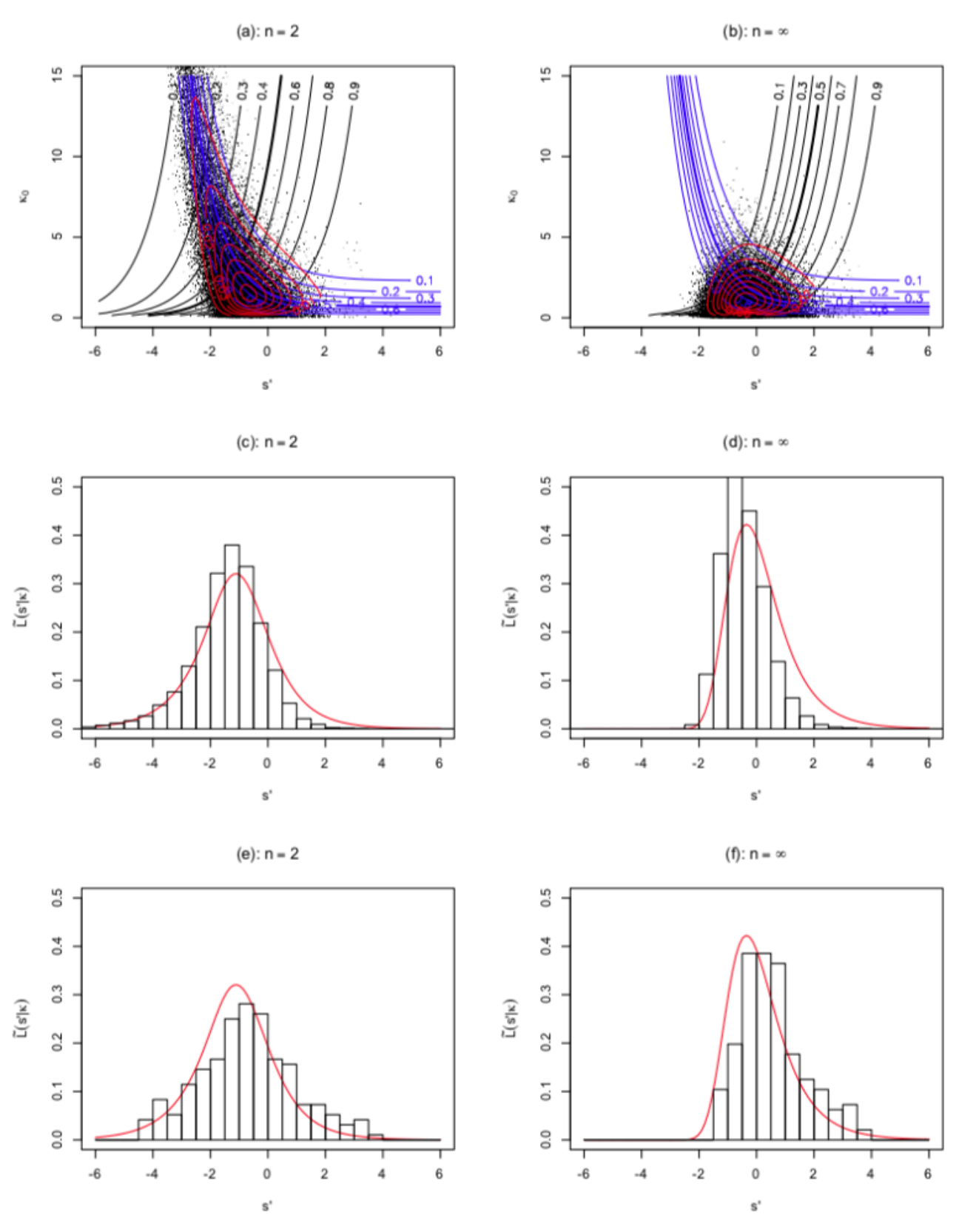
7 Numerical simulation
By exploiting the asymptotic universal functions arising from the limit we can compare the above theory with simulated data without needing to deal with explicit values of the final scaled population size .
Plotted in Fig. 6 are simulated data produced as follows. A set of trees was generated, each starting with a single ancestor and evolving as a BGW process, with each parent in the process independently producing a Poisson number of offspring with . Trees were generated until a dataset of 40000 family trees, each surviving for generations, was accumulated. For each tree individuals were randomly chosen from the final generation and their ancestry traced to locate the time of their MRCA, and to record the population size at that time. Each sample was taken from a separate tree to avoid correlations between the MRCAs of samples with a common history [4, 21]. For each family tree the time and population size corresponding to the MRCA of the entire population in the final generation was also recorded. These coalescence times and population sizes were then transformed to the scaled quantities and .
For consistency with the limit, a small number of trees with final scaled population sizes were discarded to produce the scatter plots in Figures 6(a) and (b) and the histograms of values in Figures 6(c) and (d). It is clear that the right hand tails of the histograms fall short of the theoretical marginal likelihood curves. To appreciate the cause of this discrepancy, note that the marginal likelihoods in Figures 6(c) and (d) drop to almost zero outside a finite range, . However, for practical reasons, a numerical simulation is restricted to be of finite time, namely generations, and because of this most of the trees in the sample have not existed sufficiently far in the past since the initial founder to cover this entire range. In an attempt to remedy this in Figures 6(e) and (f) we have also culled from the data all trees for which
| (56) |
This second culling is more severe, and removes the majority of generated trees. Setting , the dataset is reduced to trees satisfying , which reduces the original set to 192 trees. Nevertheless, the 2 final histograms are in closer agreement with the right hand tails of the theoretical marginal likelihoods.
8 Conclusions
We have addressed the problem of establishing confidence regions for the scaled time since coalescence to a MRCA of a random sample and the scaled population population size at the time of the MRCA under the assumption that the current observed population is the result of a BGW process that has been evolving since some unknown time in the past. Here is the number of time steps since the MRCA and is the corresponding population size. The scalings are defined in terms of the mean and variance of the number of offspring per parent. The mean is assumed to be close to and slightly larger than 1, and is assumed to be large, so that the diffusion limit can be applied. After scaling via Eq. (4) to implement the diffusion limit, the only free parameter in the problem of estimating and is the currently observed scaled population , where is the currently observed physical population size.
The approach differs markedly from earlier analyses of the MRCA in a BGW diffusion [19, 14] in that the BGW process is not initiated from a pre-specified point in the past. Lacking information about the starting conditions is not a problem for tracing ancestry in WF-like models [21] which are inherently backward-looking in time. In such models Kingman’s coalescent is immediately applicable, and the concept of a probability density for the time since a MRCA is meaningful. For a BGW process, however, causality runs forward in time, and to be on firm ground we have couched our results in terms of confidence regions. Nevertheless some interpretation is in order.
To return to the question posed in the opening paragraph of this paper, suppose we are confronted with a population which we are told has evolved through a BGW process. Although the process is stochastic and its history unknown to us, one maintains an objective belief in the existence of a single realised path through the -plane leading to the current observed scaled population , and at some point that unknown path will have passed through co-ordinates corresponding to the MRCA of the current population. Given that a BGW process is Markovian, the current population can be considered to be the result of a BGW process initiated from any point along the path, and in particular, from those co-ordinates corresponding to the MRCA. Our claim is that Eq. (44) calculated from the observed value of defines a “likelihood surface" in the sense that any subset of the -plane has a probability of containing the unknown but extant co-ordinates corresponding to the MRCA of the current population.
Having made this claim, we mention two final caveats. Firstly, note that Proposition 1 is contingent on a conjecture that the likelihood surface over the -plane is a uniform joint density. Although the marginal densities in and are uniform, this is not necessarily the case for the joint density. Indeed any density of the form where and are periodic functions of a single variable with period 1 and which integrate to zero over will have uniform marginal densities. Without further mathematical proof, uniformity of the likelihood surface over the -plane remains a conjecture.
Secondly, if the likelihood surface is well defined, one feels it should be possible, at least in principle if not in practice, to devise a numerical simulation which will confirm its interpretation. The simulation in Section 7 attempts to do this, but as we have seen, there is some ambiguity about how to match this particular simulation with theory. Devising an appropriate simulation which is guaranteed to include the MRCA of the final population but does not impose any prior constraint on the population size at the time of the MRCA remains an open problem.
Acknowledgements
CB would like to thank Robert Griffiths, Robert Clark and Francis Hui for interesting and helpful discussions.
Appendix A Derivatives of and
Derivatives of and are needed for the numerical determination of the likelihood surface defined by Eq. (44) and marginal likelihood calculation Eq. (48). Derivatives of are straightforward to calculate from Eqs. (35) and (27). Using the identity [1, p376]
| (57) |
we obtain
| (58) |
and
| (59) |
where
| (60) |
and
| (61) | |||||
From Eq. (38) the analogous derivatives for are
| (62) |
and
| (63) |
where
| (64) |
and
| (65) |
Derivatives of are less straightforward. The derivative with respect to can be calculated from the forward-Kolmogorov equation, Eq. (5), as follows;
where Eqs. (2), (27) and (57) have been used in the last line. Evaluation of the derivative of with respect to involves a numerical integration. Some straightforward but lengthy algebra gives
| (67) | |||||
Then from Eq. (39)
| (68) | |||||
where
| (69) |
References
References
- Abramowitz and Stegun [1965] Abramowitz, M., Stegun, I. A., 1965. Handbook of mathematical functions: with formulas, graphs, and mathematical tables. Dover Publications, New York.
- Athreya [2012] Athreya, K. B., 2012. Coalescence in critical and subcritical Galton-Watson branching processes. Journal of Applied Probability 49 (3), 627–638.
- Bailey [1964] Bailey, N. T. J., 1964. The elements of stochastic processes with applications to the natural sciences. Wiley, New York.
- Ball et al. [1990] Ball, R. M., Neigel, J. E., Avise, J. C., 1990. Gene genealogies within the organismal pedigrees of random-mating populations. Evolution 44 (2), 360–370.
- Burden and Simon [2016] Burden, C. J., Simon, H., 2016. Genetic drift in populations governed by a Galton–Watson branching process. Theoretical Population Biology 109, 63–74.
- Burden and Wei [2018] Burden, C. J., Wei, Y., 2018. Mutation in populations governed by a Galton–Watson branching process. Theoretical Population Biology 120, 52–61.
- Cox and Miller [1978] Cox, D. R., Miller, H. D., 1978. The theory of stochastic proceesses. Chapman and Hall, London.
- Cyran and Kimmel [2010] Cyran, K. A., Kimmel, M., 2010. Alternatives to the Wright–Fisher model: The robustness of mitochondrial Eve dating. Theoretical population biology 78 (3), 165–172.
- Durrett [1978] Durrett, R., 1978. The genealogy of critical branching processes. Stochastic Processes and their Applications 8 (1), 101–116.
- Ewens [2004] Ewens, W. J., 2004. Mathematical population genetics, 2nd Edition. Vol. 27. Springer, New York.
- Feller [1951a] Feller, W., 1951a. Diffusion processes in genetics. In: Proc. Second Berkeley Symp. Math. Statist. Prob. Vol. 227. p. 246.
- Feller [1951b] Feller, W., 1951b. Two singular diffusion problems. Annals of Mathematics 54 (1), 173–182.
- Grosjean and Huillet [2018] Grosjean, N., Huillet, T., 2018. On the genealogy and coalescence times of Bienaymé-Galton-Watson branching processes. Stochastic Models 34 (1), 1–24.
- Harris et al. [2019] Harris, S. C., Johnston, S. G., Roberts, M. I., 2019. The coalescent structure of continuous-time Galton-Watson trees. arXiv preprint arXiv:1703.00299v4.
- Kimmel and Axelrod [2015]
Kimmel, M., Axelrod, D., 2015. Branching Processes in Biology.
Interdisciplinary Applied Mathematics. Springer New York.
URL https://books.google.com.au/books?id=-ZK3BgAAQBAJ - Lambert [2003] Lambert, A., 2003. Coalescence times for the branching process. Advances in Applied Probability 35 (4), 1071–1089.
- Lambert et al. [2013] Lambert, A., Popovic, L., et al., 2013. The coalescent point process of branching trees. The Annals of Applied Probability 23 (1), 99–144.
- Le [2014] Le, V., 2014. Coalescence times for the Bienaymé-Galton-Watson process. Journal of Applied Probability 51 (1), 209–218.
- O’Connell [1995] O’Connell, N., 1995. The genealogy of branching processes and the age of our most recent common ancestor. Advances in applied probability, 418–442.
- Pardoux [2016] Pardoux, É., 2016. Probabilistic models of population evolution. Mathematical Biosciences Institute Lecture Series. Stochastics in Biological Systems. Springer, Berlin.
- Slatkin and Hudson [1991] Slatkin, M., Hudson, R. R., Oct 1991. Pairwise comparisons of mitochondrial DNA sequences in stable and exponentially growing populations. Genetics 129 (2), 555–62.
- Wolfram Research, Inc. [2019]
Wolfram Research, Inc., February 2019.
URL https://www.wolframalpha.com