\collegeordept

Physics
Department of Physics \universityLancaster University \crest [Uncaptioned image] \degreeDoctor of Philosophy in the Faculty of Science and Technology \degreedateFebruary 2019 \supervisor
Supervised by Dr David Burton and Dr Anupam Mazumdar

Infinite Derivative Gravity:
A finite number of predictions

James Edholm

Abstract

Ghost-free Infinite Derivative Gravity (IDG) is a modified gravity theory which can avoid the singularities predicted by General Relativity. This thesis examines the effect of IDG on four areas of importance for theoretical cosmologists and experimentalists. First, the gravitational potential produced by a point source is derived and compared to experimental evidence, around both Minkowski and (Anti) de Sitter backgrounds. Second, the conditions necessary for avoidance of singularities for perturbations around Minkowski and (Anti) de Sitter spacetimes are found, as well as for background Friedmann-Robertson-Walker spacetimes. Third, the modification to perturbations during primordial inflation is derived and shown to give a constraint on the mass scale of IDG, and to allow further tests of the theory. Finally, the effect of IDG on the production and propagation of gravitational waves is derived and it is shown that IDG gives almost precisely the same predictions as General Relativity for the power emitted by a binary system.

{dedication}

For my parents: Margaret and Peter

Acknowledgements.

Special thanks go to my mother Margaret, for her encouragement, and to Bonnie, for always being there to brighten my day.

I would like to particularly thank Dr David Burton, who kindly agreed to supervise me when my previous supervisor moved to a new job. David has been a tremendous help and has always been willing to guide me whenever I was stuck.

Aindriú Conroy also deserves a special mention for informally supervising me and collaborating on several papers. Aindriú was instrumental in helping my understanding of the field as well as being a true friend.

I would also like to thank the students in the Theoretical Particle Cosmology group at Lancaster who have helped me along the way: Charlotte Owen (despite her perpetual insistence on being fashionably late!), Ilia Teimouri, Spyridon Talaganis, Saleh Qutub, Leonora Donaldson-Wood & Amy Lloyd-Stubbs who all contributed greatly to my time at Lancaster.

I am also very grateful for all the friends inside and outside Lancaster who kept me motivated and supported, in particular my flatmates who (eventually!) became actual mates: Anuja, Gustaf, Sash & Craig; the other physicists: Eva, Denise, James, Marjan, Simon & Kunal; my school friends: both Ben, Chad & Will who were always ready to answer any mathematical queries with their usual attempts at humour and Dan, GB, Adam & Will who weren’t as helpful with my maths problems but always made me laugh; as well as James, Will, Sam, Tash, Robbie, Sarah, Harriet & Cat who reminded me that there was life outside the Lancaster bubble during my regular excursions to London & Bristol.

Finally my thanks go to Lancaster University for funding my research and to my viva examiners Carsten van de Bruck and John McDonald for taking the time to read my thesis and for fruitful discussions.

{declaration}

This thesis is my own work and no portion of the work referred to in this thesis has been submitted in support of an application for another degree or qualification at this or any other institute of learning.

“If I have seen further than others, it is by standing on the shoulders of giants” Isaac Newton

{pubs}

Chapter 3

•

“Behavior of the Newtonian potential for ghost-free gravity and singularity-free gravity”
J. Edholm, A. Koshelev, A. Mazumdar, arXiv:1604.01989, Physical Review D, 10.1103/PhysRevD.94.104033
•

“Newtonian potential and geodesic completeness in infinite derivative gravity”
J. Edholm, A. Conroy, arXiv:1705.02382, Physical Review D, 10.1103/PhysRevD.96.044012
•

“Revealing Infinite Derivative Gravity’s true potential: The weak-field limit around de Sitter backgrounds”
J. Edholm, arXiv:1801.00834 Physical Review D 10.1103/PhysRevD.97.064011

Chapter 4

•

“Newtonian potential and geodesic completeness in infinite derivative gravity”
J. Edholm, A. Conroy, arXiv:1705.02382, Physical Review D, 10.1103/PhysRevD.96.044012
•

“Criteria for resolving the cosmological singularity in Infinite Derivative Gravity around expanding backgrounds”
J. Edholm, A. Conroy, arXiv:1710.01366, Physical Review D, 10.1103/PhysRevD.96.124040
•

“Conditions for defocusing around more general metrics in Infinite Derivative Gravity”
J. Edholm, arXiv:1802.09063, Physical Review D, 10.1103/PhysRevD.97.084046

Chapter 5

•

“UV completion of the Starobinsky model, tensor-to-scalar ratio, and constraints on nonlocality”
J. Edholm, arXiv:1611.05062, Physical Review D 10.1103/PhysRevD.97.084046

Chapter 6

•

“Gravitational radiation in Infinite Derivative Gravity and connections to Effective Quantum Gravity”
J. Edholm, arXiv:1806.00845, Physical Review D 10.1103/PhysRevD.98.044049

Chapter 1 Introduction

Einstein’s theory of General Relativity (GR) has been extraordinarily successful at describing gravity in the hundred years since it was proposed. It predicts gravitational lensing [10], gravitational redshift [11] and gravitational waves [12]. It explains the precession of the perihelion of Mercury [13], a problem which had been unanswered for decades.

However, we do not have a full quantum completion of gravity. Gravity is not renormalizable, i.e. we cannot remove unwanted loop divergences in Feynmann diagrams, and generates singularities, or places where the spacetime curvature becomes infinite. Candidate theories such as string theory [14, 15], loop quantum gravity [16, 17] and emergent gravity [18] have not provided an overarching description of black holes or the Big Bang.

Previous classical modifications to GR include $f(R)$ gravity and finite higher-derivative terms. $f(R)$ gravity does not help with the unwanted behaviour in the ultraviolet (UV), i.e. at short distances (without fine-tuning) [19]. On the other hand, finite higher derivative theories can help with the UV behaviour, but result in terms with negative kinetic energy, known as ghosts. Ostrogradsky’s theorem of Hamiltonian analysis [20] tells us why ghosts are produced for these theories, but Infinite Derivative Gravity (IDG) is constructed specifically to avoid ghosts, by ensuring that the propagator has at most one extra pole compared to GR [21]. We will later show explicitly that IDG can be constrained so that ghosts are avoided.

1.1 What’s wrong with General Relativity?

Einstein’s great insight was to see that gravity is caused by the curvature of spacetime [22]. The simplest possible action which describes this is the Einstein-Hilbert action [22]

\displaystyle S_{\text{EH}}=\frac{1}{16\pi G}\int d^{4}x\,\sqrt{-g}R,

(1.1)

where $G$ is the gravitational constant and $R$ is the Ricci curvature scalar. $g$ is the determinant of the spacetime metric $g_{\mu\nu}$ , which we take to have the signature ( $-$ ,+,+,+) . General Relativity has successfully passed all experimental tests to date, notably predicting gravitational lensing [10] and gravitational waves [12], as well as explaining the longstanding issue of the precession of the perihelion of Mercury [13]. It is used to launch spacecraft and to enable GPS satellites to correct for gravitational redshift [11] in order to locate ourselves to an astounding level of accuracy [23].

Varying the Einstein-Hilbert action (1.1) with respect to the metric leads to the GR equations of motion

\displaystyle 8\pi G\hskip 1.42262ptT_{\mu\nu}=R_{\mu\nu}-\frac{1}{2}g_{\mu\nu}R,

(1.2)

where $R_{\mu\nu}$ is the Ricci curvature tensor and $T_{\mu\nu}$ is the stress-energy tensor which describes the distribution of matter and energy.

Despite its many successes, it was soon realised that GR predicts singularities, or divergences in the spacetime curvature. These were first thought to be anomalies or to only happen in very specific cases. It was eventually found that GR will always produce singularities due to the Penrose-Hawking singularity theorems and the Null Energy Condition (NEC) [24]. The NEC can be thought of as a covariant description of the idea that the combination of the density and the pressure of matter is a positive quantity, which applies to all matter that we have seen so far [25].

1.1.1 Previous modifications to General Relativity

The simplest modification to the GR action (1.1) is to keep the dependence on the Ricci scalar $R$ , but replace the linear dependence with a function $f(R)$ . The so-called $f(R)$ theories involve the action

\displaystyle S=\frac{1}{16\pi G}\int d^{4}x\,\sqrt{-g}f(R).

(1.3)

A notable example is Starobinsky gravity, where $f(R)=R+\alpha R^{2}$ , where $\alpha$ is a dimensionless constant, which can be used to generate cosmological inflation [26].

Unfortunately, more general modifications are plagued by the fact that ghosts are generically produced by actions which lead to equations of motion with terms with more than 2 derivatives. For example, fourth order equations of motion are produced by Stelle’s extension of GR, which is therefore commonly known as fourth order gravity and has the action [27]

\displaystyle S=\int d^{4}x\sqrt{-g}\left(M^{2}_{P}R-\alpha R^{2}+\beta R_{\mu\nu}R^{\mu\nu}\right),

(1.4)

where $M_{P}=\sqrt{\frac{1}{8\pi G}}$ is the reduced Planck mass and $\alpha$ , $\beta$ and $\gamma$ are constants. Although the action (1.4) allows renormalisation, or the removal of unwanted divergences in Feynmann diagrams [27, 28], the UV modified propagator has an additional pole compared to General Relativity when the momentum $k_{\mu}$ satisfies $k^{\mu}k_{\mu}=\frac{M^{2}_{P}}{2\left(\beta-3\alpha\right)}$ [27]. This extra pole has a negative residue and therefore is an excitation with negative kinetic energy, known as a ghost [29].

Notably $f(R)$ gravity escapes this fate because such theories can be described by a single extra scalar degree of freedom added to GR, which does not necessarily lead to a ghost.

Classically speaking, tachyons are another cause for concern in modified gravity theories. Particles with imaginary mass will travel faster than light [30], so to avoid this fate we can only introduce poles at $k^{2}+m^{2}$ with real mass $m^{2}\geq 0$ .

1.1.2 Other modified gravity theories

In four spacetime dimensions, the Gauss-Bonnet term $G=R^{2}-4R^{\mu\nu}R_{\mu\nu}+R^{\mu\nu\rho\sigma}R_{\mu\nu\rho\sigma}$ is a topological surface term and so adding it to the Einstein-Hilbert action has no effect on the equations of motion. (1.4) is sometimes written with an extra term $\gamma R^{\mu\nu\rho\sigma}R_{\mu\nu\rho\sigma}$ , but the action can be separated into (1.4) and the surface term. The $d$ -dimensional action

\displaystyle S=\int d^{d}x\sqrt{-g}\left(M^{2}_{P}R+R^{2}-4R^{\mu\nu}R_{\mu\nu}+R^{\mu\nu\rho\sigma}R_{\mu\nu\rho\sigma}\right),

(1.5)

is known as Gauss-Bonnet gravity, which only modifies gravity in 5 or more spacetime dimensions.

1.2 Motivation for infinite derivatives

The Ostrogradsky instability produces a ghost for a generic theory where a finite number of higher derivatives (more than 2) act on terms in the action [20]. This however does not apply when there are an infinite number of derivatives. These infinite derivatives were first used in string theory in order to avoid singularities [31] before being applied to gravity [32, 33].

The most general quadratic¹¹ 1 We look here only at quadratic curvatures, but future work could look at the effect of cubic or higher order curvatures. covariant, parity-invariant, metric-compatible, torsion-free action is [33]

	$\displaystyle S_{\text{IDG}}$	$\displaystyle=$	$\displaystyle\int d^{4}x\,\frac{\sqrt{-g}}{2}\Big[M^{2}_{P}R+RF_{1}(\Box)R+R_{\mu\nu}F_{2}(\Box)R^{\mu\nu}+R_{\mu\nu\rho\sigma}F_{3}(\Box)R^{\mu\nu\rho\sigma}\Big],$		(1.6)
			$\displaystyle\text{with}\quad F_{i}(\Box)=\sum^{\infty}_{n=0}f_{i_{n}}\frac{\Box^{n}}{M^{2n}}\,,$		(1.6)

where { $f_{i_{0}},f_{i_{1}},f_{i_{2}},...,f_{i_{n}}$ } are dimensionless coefficients and $\Box=g^{\mu\nu}\nabla_{\mu}\nabla_{\nu}$ is the d’Alembertian operator.²² 2 Each $\Box$ term comes with an associated mass scale $M^{2}$ , where $M<M_{p}=(16\pi G)^{-1/2}\sim 2.4\times 10^{18}$ GeV. The physical significance of $M$ could be any scale beyond $10^{-2}$ eV, which arises from constraints on studying the $1/r$ -fall of the Newtonian potential [3]. When writing the $F_{i}(\Box)$ , we suppress the scale $M$ in order to simplify our formulae for the rest of this thesis. However, for any physical comparison one has to bring in the scale $M$ along with $M_{p}$ . $M$ is a new mass scale, which together with the $f_{i_{n}}$ s regulates the length scale at which the higher derivative terms start to have a significant effect.

The IDG action has been the subject of many papers in the past decade, with researchers looking at the bending of light round the sun [34, 35], exact solutions of the theory [36], the diffusion equation [37, 38], black hole stability [39], causality [40], and time reflection positivity [41].

It was shown in [42] that the initial value problem is well-posed even when there are infinitely many derivatives and that only a finite number of initial conditions are required. Exact plane wave solutions to IDG were studied in [43]. In the time since this thesis was submitted for viva voce examination, more papers have been released looking at the stability of the Minkowski spacetime [44] and the Casimir effect [45].

1.3 Summary of previous results

In this section we give a brief summary of the aspects of Infinite Derivative Gravity which are not covered in the rest of this thesis but are nevertheless important in their own right.

1.3.1 Entropy

The entropy $S_{\text{BH}}$ of an axisymmetric black hole was famously found by Bekenstein and Hawking to depend on the area of the black hole event horizon [46, 47], with the exact form

\displaystyle S_{\text{BH}}=\frac{\text{Area}}{4G}.

(1.7)

It was found in [48] that in the linear regime, this formula was not modified by the addition of the extra terms in the IDG action, given the necessary constraints to avoid introducing any extra degrees of freedom into the propagator, although there are corrections at the non-linear level. It was further found in [49] that the entropy of a rotating Kerr black hole was not modified by the Ricci scalar or Ricci tensor terms in (1.6), but there would be corrections from the Riemann tensor term.

In [50], the entropy around an (Anti) de Sitter, or (A)dS, metric in D-dimensions was calculated, giving us constraints on the coefficients in the action (1.6), which later help us when calculating the conditions to avoid singularities.

1.3.2 Boundary terms of the theory

The Einstein-Hilbert action contains second derivatives of the metric, so in theory one would need to fix the metric and its derivatives on the boundary of any spacetime manifold. However, the Gibbons-Hawking-York (GHY) boundary terms for GR were found in 1977. The GHY boundary cancels out the terms generated by the EH action on the boundary [51, 52]. The IDG boundary terms were found in [53] using the Arnowitt-Deser-Miser (ADM) decomposition [54], which splits the spacetime metric into spatial slices of constant time, followed by a coframe slicing, which leads to a simpler line element. This was first done for the example of an infinite derivative scalar field, before extending the method to the gravitational case. To use the d’Alembertian operator in the coframe, it was necessary to split it into a spatial derivative operator and a time derivative operator.

It was shown in [55] that for a general action depending on the Riemann tensor $R_{\mu\nu\rho\sigma}$ or its contractions

\displaystyle S=\frac{1}{16\pi G}\int_{\mathcal{M}}d^{4}x\,\sqrt{-g}f(R_{\mu\nu\rho\sigma})\,,

(1.8)

it is possible to add the auxiliary fields $\varrho_{\mu\nu\rho\sigma}$ and $\varphi^{\mu\nu\rho\sigma}$ . These fields are independent of the metric and of each other, but retain the symmetries of the Riemann tensor. This allows us to write the action (1.6) as

\displaystyle S=\frac{1}{16\pi G}\int_{\mathcal{M}}d^{4}x\,\sqrt{-g}\left[f(\varrho_{\mu\nu\rho\sigma})+\varphi^{\mu\nu\rho\sigma}\left(R_{\mu\nu\rho\sigma}-\varrho_{\mu\nu\rho\sigma}\right)\right]\,.

(1.9)

After a long and technical calculation laid out in [53], we are able to find the total derivative term in the action by using the Gauss, Codazzi and Ricci equations as well as the equations of motion for the auxiliary fields. As the boundary term is defined as the term needed to cancel out the total derivative term in the action, therefore we arrive at the IDG boundary terms

$\displaystyle S_{tot}$	$\displaystyle=$	$\displaystyle S_{gravity}+S_{boundary}$	(1.10)
	$\displaystyle=$	$\displaystyle\frac{1}{16\pi G}\int_{\mathcal{M}}d^{4}x\,\sqrt{-g}\Big[\varrho+\alpha\big(\varrho F_{1}(\Box)\varrho+\varrho_{\mu\nu}F_{2}(\Box)\varrho^{\mu\nu}$
		$\displaystyle+\varrho_{\mu\nu\rho\sigma}F_{3}(\Box)\varrho^{\mu\nu\rho\sigma}\big)+\varphi^{\mu\nu\rho\sigma}\left(R_{\mu\nu\rho\sigma}-\varrho_{\mu\nu\rho\sigma}\right)\Big]$
		$\displaystyle+\frac{1}{8\pi G}\oint_{\partial\mathcal{M}}d\Sigma_{\mu}\,n^{\mu}\Big[K+\alpha\big(2KF_{1}(\Box)\rho-4KF_{1}(\Box)\Omega-KF_{2}(\Box)\Omega$
		$\displaystyle-\left.\left.K_{ij}F_{2}(\Box)\Omega^{ij}+K_{ij}F_{2}(\Box)\rho^{ij}-4K_{ij}F_{3}(\Box)\Omega^{ij}-2\Omega_{ij}X_{1}^{ij}-\frac{1}{2}\Omega_{ij}X_{2}^{ij}\right)\right],\penalty\ \penalty\ \penalty\ \penalty\ \penalty\ \penalty\ \penalty\ \penalty\ \penalty\$

where $\Omega_{ij}=n^{\gamma}n^{\delta}\varrho_{\gamma i\delta j}$ is the contraction of the auxiliary field with $n^{\mu}$ , the normal vector to the ADM hypersurface and $K_{ij}=-\nabla_{i}n_{j}$ is the extrinsic curvature of the hypersurface. The $X_{ij}$ terms are additional terms which appear due to the existence of the d’Alembertian in the action and depend on the choice of coframe slicing. It is notable that the $F(\Box)$ terms feature in the boundary - the infinite derivative terms filter through from the bulk.

The fact that the boundary terms can be found is a useful check on the theory. The method of finding the boundary terms can also be used when calculating the Hamiltonian of the theory.

1.3.3 Hamiltonian analysis of the theory

By examining the propagator of the theory, we will later show using Lagrangian analysis that there will be no ghost degrees of freedom. Intuitively, one would expect the same thing from a Hamiltonian analysis, but it is reassuring to study it explicitly.

By starting with a toy model of an infinite derivative scalar field and using the ADM decomposition, it is possible to find the Hamiltonian and the constraints that arise [56]. It is pleasing to see that one can show that by choosing the coefficients in the action correctly, we can make sure there are no extra poles in the theory compared to GR.

1.3.4 Quantum aspects of the theory

The unitarity of the theory, i.e. the requirement that the sum of all possible outcomes is equal to unity, was examined in [57] and the Slavnov identities found in [58]. It was shown that the mass scale of the theory could vary depending on the number of particles in the system [59], so that the effective mass scale would be inversely proportional to the square root of the number of particles.

By looking at an infinite derivative scalar toy model, it was shown that one could cancel the divergences in one-loop scattering diagrams and that the exponential suppression of the propagator could aid convergence [60, 61]. The behaviour of the 2-loop, 2-point function can also be controlled [61]. It was shown that one-particle irreducible (1PI) Feynmann diagrams could be made UV finite (i.e. does not diverge in the ultraviolet, or high energy, regime) by using an infinite derivative scalar toy model [62]. For those wanting a more detailed understanding of the quantum aspects of IDG, the review paper [63] may be helpful.

Renormalisibility of the theory was also studied in more general dimensions (i.e. a number spacetime dimensions not equal to four) [64, 65], which found that IDG could be described as super-renormalisable.

1.3.5 Using IDG as a source for the accelerated expansion of the universe

Refer to caption — Figure 1.1: A plot of the gravitational potential against the distance from a source in different models. The different curves represent the standard GR prediction, the exponential choice of form factors (1.13) [1] and the pure Yukawa suppression of massive gravity for comparison. The authors chose a mass of 1m^-1 for the massive gravity and exponential curves.

In this thesis, we use IDG to suppress the strength of gravity at small scales in order to avoid singularities. However, they can also be used to produce effects at large distances.

Infinite derivatives, in the form of a infinite series of the inverse d’Alembertian $1/\Box$ , have been been used to explain the accelerated expansion of the universe. This acceleration, first observed in the 1990s, requires either some unknown “dark energy” (normally assumed to have the form of a cosmological constant $\Lambda$ ) to drive expansion or modifications to the gravitational action [66, 67, 68].

Massive gravity actions extend the Einstein-Hilbert action (1.1) with terms of the form $\frac{m_{gr}^{2}}{\Box^{2}}R$ , where $m_{gr}$ is the non-zero mass of the graviton [69, 70, 71, 72, 73, 74].

An infinite series of inverse d’Alembertian operators were used to generate the accelerated expansion in [1]. The authors used inverse d’Alembertian operators instead of d’Alembertians, so that the action took the form of (1.6) with the $F_{i}(\Box)$ replaced with

\displaystyle\bar{F}_{i}(\Box)=\sum_{n=1}^{\infty}f_{i_{-n}}(M^{2}/\Box)^{n},

(1.11)

where the $f_{i_{-n}}$ are dimensionless coefficients. The non-linear field equations were found, allowing the authors to derive the Newtonian potential at large distances shown in Fig. 1.1. For this plot, the form factors (terms which appear in the equations of motion)

	$\displaystyle\bar{a}(\Box)$	$\displaystyle\equiv$	$\displaystyle 1+M^{-2}_{P}\left(\frac{1}{2}\bar{F}_{2}(\Box)+\bar{F}_{3}(\Box)\right)\Box,$
	$\displaystyle\bar{c}(\Box)$	$\displaystyle\equiv$	$\displaystyle 1+M^{-2}_{P}\left(-2\bar{F}_{1}(\Box)-\frac{1}{2}\bar{F}_{2}(\Box)+\frac{1}{3}\bar{F}_{3}(\Box)\right)\Box,$		(1.12)

were chosen so that

\displaystyle\bar{a}(\Box)=\bar{c}(\Box)=\exp(-M^{2}/\Box).

(1.13)

The authors of [1] found that the choice (1.13) gave two modifications to the Newtonian potential. Firstly, similar to other massive gravity theories, the potential was exponentially suppressed at large distances.Secondly, the potential was modified by an oscillating factor $\cos(Mr)$ . This would allow IDG to be differentiated from other massive gravity theories by observations.

1.4 Organisation of thesis

The content of this thesis is organised as follows:

Chapter 2: We show that the IDG action can be derived from the most general metric-based, torsion-free, quadratic in curvature action. We give the full non-linear equations of motion and use these to derive the equations of motion around a flat background and an (Anti) de Sitter, or (A)dS background. Finally we find the propagator around a Minkowski background, giving the necessary conditions to avoid ghosts, and give the quadratic variation of the action around maximally symmetric backgrounds (Minkowski and (A)dS), which we later use to investigate perturbations in the Cosmic Microwave Background.

Chapter 3: We find the Newtonian potential, which is the perturbation to a background metric caused by a static, spherically symmetric point source. We first look at a perturbation around a flat background and use this to constrain our mass scale as well as show that we return to the GR prediction at large distances. We later look at a de Sitter background and show that using the Minkowski metric as a background is an acceptable approximation for a de Sitter background with the current Hubble parameter.

Chapter 4: We examine the concept of a singularity and how GR will always generate geometric singularities due to the Hawking-Penrose singularity theorems. This is because GR requires null rays to focus, which means that one cannot trace the path of light to past infinity, known as geodesic incompleteness. We show how IDG can avoid this fate by fulfilling the defocusing conditions, both for perturbations around Minkowski & (A)dS backgrounds, and for a background Friedmann-Robertson-Walker (FRW) solution, thus solving the Big Bang Singularity Problem.

Chapter 5: IDG can be thought of as an extension to Starobinsky inflation and we show how this changes the inflationary observables in the Cosmic Microwave Background. This allows us to use data from the Planck satellite to place further constraints on our mass scale.

Chapter 6: We examine how IDG affects the production and propagation of gravitational radiation. First we derive the modified quadrupole formula, then look at the backreaction produced by the emission of gravitational waves and give a prediction for the power produced by a system. We take the example of a binary system in both a circular and an elliptical orbit and use the Hulse-Taylor binary to constrain our mass scale.

Chapter 2 Infinite Derivative Gravity

2.1 Infinite Derivative Gravity

We begin by deriving the action (1.6). Here we look at the derivation around Minkowski spacetime [75], but the calculation can also be carried out in a maximally symmetric spacetime such as (Anti) de Sitter [76]. Our starting point is the most general, quadratic in curvature, covariant, metric-tensor based modification to the Einstein-Hilbert action in four dimensions, which is given by [75]

\displaystyle S=\int d^{4}x\sqrt{-g}\left(R_{\mu_{1}\nu_{1}\lambda_{1}\sigma_{1}}\mathcal{O}^{\mu_{1}\nu_{1}\lambda_{1}\sigma_{1}}_{\mu_{2}\nu_{2}\lambda_{2}\sigma_{2}}R^{\mu_{2}\nu_{2}\lambda_{2}\sigma_{2}}\right),

(2.1)

where the operator $\mathcal{O}^{\mu_{1}\nu_{1}\lambda_{1}\sigma_{1}}_{\mu_{2}\nu_{2}\lambda_{2}\sigma_{2}}$ is a general covariant operator and all the possible Riemannian curvatures (Riemann, Weyl and Ricci tensors and Ricci scalar) are represented by $R_{\mu_{1}\nu_{1}\lambda_{1}\sigma_{1}}$ .

In full, (2.1) is given by¹¹ 1 There is no term of the form $F(\Box)R$ as this would be a total derivative and therefore equivalent to a boundary term. [75]

$\displaystyle S$	$\displaystyle=$	$\displaystyle\int d^{4}x\frac{\sqrt{-g}}{2}\Big[M_{P}^{2}R+RF_{1}(\Box)R+RF_{2}(\Box)\nabla_{\nu}\nabla_{\mu}R^{\mu\nu}+R_{\mu\nu}F_{3}(\Box)R^{\mu\nu}$	(2.2)
	$\displaystyle+$	$\displaystyle R_{\mu}^{\nu}F_{4}(\Box)\nabla_{\nu}\nabla_{\lambda}R^{\mu\lambda}+R^{\lambda\sigma}F_{5}(\Box)\nabla_{\mu}\nabla_{\sigma}\nabla_{\nu}\nabla_{\lambda}R^{\mu\nu}+RF_{6}(\Box)\nabla_{\mu}\nabla_{\nu}\nabla_{\lambda}\nabla_{\sigma}R^{\mu\nu\lambda\sigma}$
	$\displaystyle+$	$\displaystyle R_{\mu\lambda}F_{7}(\Box)\nabla_{\nu}\nabla_{\sigma}R^{\mu\nu\lambda\sigma}+R_{\lambda}^{\rho}F_{8}(\Box)\nabla_{\mu}\nabla_{\sigma}\nabla_{\nu}\nabla_{\rho}R^{\mu\nu\lambda\sigma}$
	$\displaystyle+$	$\displaystyle R^{\mu_{1}\nu_{1}}F_{9}(\Box)\nabla_{\mu_{1}}\nabla_{\nu_{1}}\nabla_{\mu}\nabla_{\nu}\nabla_{\lambda}\nabla_{\sigma}R^{\mu\nu\lambda\sigma}+R_{\mu\nu\lambda\sigma}F_{10}(\Box)R^{\mu\nu\lambda\sigma}$
	$\displaystyle+$	$\displaystyle R^{\rho}{}_{\mu\nu\lambda}F_{11}(\Box)\nabla_{\rho}\nabla_{\sigma}R^{\mu\nu\lambda\sigma}+R_{\mu\rho_{1}\nu\sigma_{1}}F_{12}(\Box)\nabla^{\rho_{1}}\nabla^{\sigma_{1}}\nabla_{\rho}\nabla_{\sigma}R^{\mu\rho\nu\sigma}$
	$\displaystyle+$	$\displaystyle R_{\mu}^{\;\nu_{1}\rho_{1}\sigma_{1}}F_{13}(\Box)\nabla_{\rho_{1}}\nabla_{\sigma_{1}}\nabla_{\nu_{1}}\nabla_{\nu}\nabla_{\lambda}\nabla_{\sigma}R^{\mu\nu\lambda\sigma}$
	$\displaystyle+$	$\displaystyle R^{\mu_{1}\nu_{1}\rho_{1}\sigma_{1}}F_{14}(\Box)\nabla_{\rho_{1}}\nabla_{\sigma_{1}}\nabla_{\nu_{1}}\nabla_{\mu_{1}}\nabla_{\mu}\nabla_{\nu}\nabla_{\lambda}\nabla_{\sigma}R^{\mu\nu\lambda\sigma}\Big]\,.$

We can simplify (2.2) by commuting derivatives, recalling that we are examining fluctuations around a Minkowski background. Additionally, the antisymmetric nature of the Riemann tensor (A.4) and the (second) Bianchi identity (A.10) allow us to write the action in a simplified form. For example, we can commute the $\mu$ and $\nu$ indices in the $F_{6}(\Box)$ term as follows

$\displaystyle\nabla_{\mu}\nabla_{\nu}\nabla_{\lambda}\nabla_{\sigma}R^{\mu\nu\lambda\sigma}$	$\displaystyle=$	$\displaystyle\frac{1}{2}\left[\nabla_{\mu}\nabla_{\nu}\nabla_{\lambda}\nabla_{\sigma}R^{\mu\nu\lambda\sigma}+\nabla_{\nu}\nabla_{\mu}\nabla_{\lambda}\nabla_{\sigma}R^{\mu\nu\lambda\sigma}\right]$	(2.3)
	$\displaystyle=$	$\displaystyle\frac{1}{2}\left[\nabla_{\mu}\nabla_{\nu}\nabla_{\lambda}\nabla_{\sigma}R^{\mu\nu\lambda\sigma}+\nabla_{\mu}\nabla_{\nu}\nabla_{\lambda}\nabla_{\sigma}R^{\nu\mu\lambda\sigma}\right]$
	$\displaystyle=$	$\displaystyle 0.$

where we relabeled the indices on the second term to get to the second line and used the antisymmetry of the Riemann tensor to get to the third line. By repeating this procedure for the other terms, we can write (2.2) as (1.6), i.e. [75]

	$\displaystyle S$	$\displaystyle=$	$\displaystyle\int d^{4}x\,\frac{\sqrt{-g}}{2}\Big[M^{2}_{P}R+RF_{1}(\Box)R+R_{\mu\nu}F_{2}(\Box)R^{\mu\nu}+R_{\mu\nu\rho\sigma}F_{3}(\Box)R^{\mu\nu\rho\sigma}\Big],$		(2.4)
			$\displaystyle\text{with}\quad F_{i}(\Box)=\sum^{\infty}_{n=0}f_{i_{n}}\frac{\Box^{n}}{M^{2n}}\,.$		(2.4)

2.1.1 Equations of motion

We are now ready to derive the equations of motion for the Infinite Derivative Gravity action (2.4), following the method of [77]. Using the identities in Appendix A.1.3 and Appendix A.1.4, one can proceed by varying the action to find the gravitational stress energy tensor $T^{\mu\nu}$

\displaystyle T^{\mu\nu}\equiv-\frac{2}{\sqrt{-g}}\frac{\delta S}{\delta g_{\mu\nu}}.

(2.5)

The full equations of motion for the action (1.6) are given by [77]

$\displaystyle T^{\alpha\beta}$	$\displaystyle=$	$\displaystyle M^{2}_{P}G^{\alpha\beta}+2G^{\alpha\beta}F_{1}(\Box)R+2g^{\alpha\beta}RF_{1}(\Box)R-2\left(\nabla^{\alpha}\nabla^{\beta}-g^{\alpha\beta}\Box\right)F_{1}(\Box)R$	(2.6)
		$\displaystyle-\Omega^{\alpha\beta}_{1}+\frac{1}{2}g^{\alpha\beta}\left(\Omega^{\sigma}_{1\sigma}+\bar{\Omega}_{1}\right)+2{R^{(\beta}}_{\mu}F_{2}(\Box)R^{\mu\alpha)}-\frac{1}{2}g^{\alpha\beta}R^{\mu\nu}F_{2}(\Box)R_{\mu\nu}$
		$\displaystyle-2\nabla^{(\alpha}\nabla_{\mu}F_{2}(\Box)R^{\mu\beta)}+\Box F_{2}(\Box)R^{\alpha\beta}+g^{\alpha\beta}\nabla_{\mu}\nabla_{\nu}F_{2}(\Box)R^{\mu\nu}-\Omega^{\alpha\beta}_{2}$
		$\displaystyle+\frac{1}{2}g^{\alpha\beta}\left(\Omega^{\sigma}_{2\sigma}+\bar{\Omega}_{2}\right)-2\Delta^{\alpha\beta}_{2}-\frac{1}{2}g^{\alpha\beta}C^{\mu\nu\lambda\sigma}F_{3}(\Box)C_{\mu\nu\lambda\sigma}+2{C^{\alpha}}_{\rho\theta\psi}F_{3}(\Box)C^{\beta\rho\theta\psi}$
		$\displaystyle-2\left[2\nabla_{\mu}\nabla_{\nu}+R_{\mu\nu}\right]F_{3}(\Box)C^{\beta\mu\nu\alpha}-\Omega^{\alpha\beta}_{3}+\frac{1}{2}g^{\alpha\beta}\left(\Omega^{\gamma}_{3\gamma}+\bar{\Omega}_{3}\right)-4\Delta^{\alpha\beta}_{3},$

where the $C_{\mu\nu\rho\sigma}$ is the Weyl curvature tensor and we have defined

$\displaystyle\Omega^{\alpha\beta}_{1}$	$\displaystyle=$	$\displaystyle\sum^{\infty}_{n=1}f_{1_{n}}\sum^{n-1}_{l=0}\nabla^{\alpha}\Box^{l}R\nabla^{\beta}\Box^{(n-l-1)}R,\quad\bar{\Omega}_{1}=\sum^{\infty}_{n=1}f_{1_{n}}\sum^{n-1}_{l=0}\Box^{l}R\Box^{(n-l)}R,$
$\displaystyle\Omega_{2}^{\alpha\beta}$	$\displaystyle=$	$\displaystyle\sum^{\infty}_{n=1}f_{2_{n}}\sum^{n-1}_{l=0}\nabla_{\nu}\left[\Box^{l}R^{\nu}_{\sigma}\Box^{(n-l-1)}R^{(\beta\|\sigma\|;\alpha)}-\Box^{l}R^{\nu;(\alpha}_{\sigma}\Box^{(n-l-1)}R^{\beta)\sigma}\right],$
$\displaystyle\Delta_{2}^{\alpha\beta}$	$\displaystyle=$	$\displaystyle\sum_{n=1}^{\infty}f_{2_{n}}\sum_{l=0}^{n-1}\nabla_{\nu}\left[\Box^{l}R^{\nu}_{\sigma}\nabla^{(\alpha}\Box^{(n-l-1)}R^{\beta)\sigma}-\nabla^{(\alpha}\Box^{l}R^{\nu}_{\sigma}\Box^{(n-l-1)}R^{\nu\sigma}\right],$
$\displaystyle\Omega^{\alpha\beta}_{3}$	$\displaystyle=$	$\displaystyle\sum^{\infty}_{n=1}f_{3_{n}}\sum^{n-1}_{l=0}\nabla^{\alpha}\Box^{l}C^{\mu}{}_{\nu\lambda\sigma}\nabla^{\beta}\Box^{(n-l-1)}{C_{\mu}}^{\nu\lambda\sigma},\quad\bar{\Omega}_{3}=\sum_{n=1}^{\infty}f_{3_{n}}\sum^{n-1}_{l=0}\Box^{l}C^{\mu}{}_{\nu\lambda\sigma}\Box^{n-1}C_{\mu}{}^{\nu\lambda\sigma},$
$\displaystyle\Delta^{\alpha\beta}_{3}$	$\displaystyle=$	$\displaystyle\frac{1}{2}\sum_{n=1}^{\infty}f_{3_{n}}\sum^{n-1}_{l=0}\nabla_{\nu}\left[\Box^{l}C^{\lambda\nu}{}_{\sigma\mu}\nabla^{(\alpha}\Box^{(n-l-1)}{C_{\lambda}}^{\beta)\sigma\mu}-\nabla^{(\alpha}\Box^{l}C^{\lambda\nu}{}_{\sigma\mu}C_{\lambda}{}^{\beta)\sigma\mu(n-l-1)}\right].\penalty\ \penalty\ \penalty\ \penalty\ \penalty\ \penalty\ \penalty\ \penalty\$	(2.7)

As expected, these equations satisfy the generalised Bianchi identities
$\nabla^{\alpha}T_{\alpha\beta}=0$ . This is because the action (2.4) is metric-based, and any metric-based Lagrangian will be diffeomorphism invariant and therefore satisfy the generalised Bianchi identities [78].

By contracting (2.6) with $g_{\alpha\beta}$ , we find that the trace equation is

	$\displaystyle T$	$\displaystyle=$	$\displaystyle g_{\alpha\beta}T^{\alpha\beta}=-M^{2}_{P}R+6\Box F_{1}(\Box)R+\Omega^{\sigma}_{1\sigma}+2\bar{\Omega}_{1}-2\nabla_{\mu}\nabla_{\nu}\left(F_{2}(\Box)R^{\mu\nu}\right)+\Omega^{\sigma}_{2\sigma}$		(2.8)
			$\displaystyle+2\bar{\sigma}_{2}-2\Delta^{\alpha}_{2\alpha}-2C^{\mu\nu\lambda\sigma}F_{3}(\Box)C_{\mu\nu\lambda\sigma}+2C_{\beta\mu\nu\sigma}F_{3}(\Box)C^{\beta\mu\nu\sigma}+\Omega^{\gamma}_{3\gamma}+2\bar{\Omega}_{3}-4\Delta^{\alpha}_{3\alpha.}\penalty\ \penalty\ \penalty\ \penalty\ \penalty\ \penalty\ \penalty\ \penalty\$		(2.8)

2.2 Equations around various backgrounds

We now simplify the equations by linearising around specific backgrounds. We assume a background solution $\bar{g}_{\mu\nu}$ and then make a small variation $h_{\mu\nu}$ , so that²² 2 We define $h^{\mu\nu}=-\delta g^{\mu\nu}$ , which follows from the requirement that the Kronecker delta is invariant under a linear variation to the metric, up to linear order in the variation [29]. $g_{\mu\nu}\to\bar{g}_{\mu\nu}+h_{\mu\nu}$ , $g^{\mu\nu}\to\bar{g}^{\mu\nu}-h^{\mu\nu}$ . We later use the linear equations of motion to see what happens for perturbations caused by a small amount of matter, or random fluctuations caused by quantum effects.

2.2.1 Equations around a flat background

For a flat background, we can make two simplifications. Firstly, the background curvatures are zero, so any terms in (2.6) which are quadratic in the curvatures will not contribute to the linearised equations of motion. Secondly, for linearised perturbations around a flat background, covariant derivatives commute.

For the perturbed metric $g_{\mu\nu}\to\eta_{\mu\nu}+h_{\mu\nu}$ , $g^{\mu\nu}\to\eta^{\mu\nu}-h^{\mu\nu}$ , we can write the linearised equations of motion as [75]

$\displaystyle T^{\alpha\beta}$	$\displaystyle=$	$\displaystyle M^{2}_{P}\left(r^{\alpha\beta}-\frac{1}{2}g^{\alpha\beta}r\right)-2\left(\nabla^{\alpha}\nabla^{\beta}-g^{\alpha\beta}\bar{\Box}\right)F_{1}(\bar{\Box})r$	(2.9)
		$\displaystyle-2\nabla^{(\alpha}\nabla_{\mu}F_{2}(\bar{\Box})r^{\mu\beta)}+\bar{\Box}F_{2}(\bar{\Box})r^{\alpha\beta}+g^{\alpha\beta}\nabla_{\mu}\nabla_{\nu}F_{2}(\bar{\Box})r^{\mu\nu}$
		$\displaystyle-4\nabla_{\mu}\nabla_{\nu}F_{3}(\bar{\Box})c^{\beta\mu\nu\alpha},$

where the background d’Alembertian is denoted by $\bar{\Box}$ , $c_{\mu\nu\rho\sigma}$ is the linearised Weyl tensor, and the linearised Riemann and Ricci curvatures around a flat background are

	$\displaystyle r_{\rho\mu\sigma\nu}=\frac{1}{2}\left(\partial_{\sigma}\partial_{\mu}h_{\rho\nu}+\partial_{\nu}\partial_{\rho}h_{\mu\sigma}-\partial_{\nu}\partial_{\mu}h_{\rho\sigma}-\partial_{\sigma}\partial_{\rho}h_{\mu\nu}\right),$
	$\displaystyle r_{\mu\nu}=\frac{1}{2}\left(\partial_{\sigma}\partial_{\mu}h^{\sigma}_{\nu}+\partial_{\nu}\partial_{\sigma}h^{\sigma}_{\mu}-\partial_{\nu}\partial_{\mu}h-\bar{\Box}h_{\mu\nu}\right),$
	$\displaystyle r=\partial_{\mu}\partial_{\nu}h^{\mu\nu}-\bar{\Box}h.$		(2.10)

We can write (2.9) in the simplified form

\displaystyle\frac{1}{M^{2}_{P}}T_{\mu\nu}

\displaystyle=

\displaystyle a(\bar{\Box})r_{\mu\nu}-\frac{1}{2}g_{\mu\nu}c(\bar{\Box})r-\frac{1}{2}\partial_{\mu}\partial_{\nu}f(\bar{\Box})r,

(2.11)

where the functions $a(\Box)$ , $c(\Box)$ and $f(\Box)$ are defined as

$\displaystyle a(\bar{\Box})$	$\displaystyle=$	$\displaystyle 1+M^{-2}_{P}\bigg(F_{2}(\bar{\Box})+2F_{3}(\bar{\Box})\bigg)\bar{\Box},$
$\displaystyle c(\bar{\Box})$	$\displaystyle=$	$\displaystyle 1+M^{-2}_{P}\left(-4F_{1}(\bar{\Box})-F_{2}(\bar{\Box})+\frac{2}{3}F_{3}(\bar{\Box})\right)\bar{\Box},$
$\displaystyle f(\bar{\Box})$	$\displaystyle=$	$\displaystyle M^{-2}_{P}\left(4F_{1}(\bar{\Box})+2F_{2}(\bar{\Box})+\frac{4}{3}F_{3}(\bar{\Box})\right).$	(2.12)

Note that $\bar{\Box}f(\bar{\Box})=a(\bar{\Box})-c(\bar{\Box})$ and that contracting (2.11) with $g^{\mu\nu}$ leads to the trace equation of motion around Minkowski spacetime

\displaystyle\frac{1}{M^{2}_{P}}T

\displaystyle=

\displaystyle\frac{1}{2}\left(a(\bar{\Box})-3c(\bar{\Box})\right)r.

(2.13)

In terms of the perturbation to the metric $h_{\mu\nu}$ , (2.11) can be written as [29]

	$\displaystyle-2\kappa T_{\mu\nu}\hskip-5.69054pt$	$\displaystyle=$	$\displaystyle\hskip-5.69054pta(\bar{\Box})\left(\bar{\Box}h_{\mu\nu}\hskip-2.27621pt-\hskip-2.27621pt\partial_{\sigma}\left(\partial_{\mu}h^{\sigma}_{\nu}+\partial_{\nu}h^{\sigma}_{\mu}\right)\right)+c(\bar{\Box})\left(\partial_{\mu}\partial_{\nu}h+\eta_{\mu\nu}\partial_{\sigma}\partial_{\tau}h^{\sigma\tau}-\eta_{\mu\nu}\bar{\Box}h\right)$		(2.14)
			$\displaystyle+f(\bar{\Box})\hskip 2.84526pt\partial_{\mu}\partial_{\nu}\partial_{\sigma}\partial_{\tau}h^{\sigma\tau},$		(2.14)

where $\kappa=M^{-2}_{P}$ .

2.2.2 Equations around a de Sitter background

The de Sitter (dS) metric is a subset of the general FRW metric (4.30) with the scale factor $a(t)=e^{Ht}$ where $H$ , the Hubble parameter $H=\frac{\dot{a}}{a}$ , is a constant here. The scale factor is a dimensionless quantity which describes the evolution of proper distance between two locally stationary objects. The line element can be written as

\displaystyle ds^{2}=-dt^{2}+e^{2Ht}\left(dx^{2}+dy^{2}+dz^{2}\right).

(2.15)

The dS metric has the property of being maximally symmetric, which for 4 spacetime dimensions means that there are 10 Killing vectors [78]. We therefore have the constant background curvatures

\displaystyle\bar{R}^{\mu}{}_{\nu\rho\sigma}=\frac{\bar{R}}{12}\left(\delta^{\mu}_{\rho}g_{\nu\sigma}-\delta^{\mu}_{\sigma}g_{\nu\rho}\right),\quad\bar{R}^{\mu}_{\nu}=\frac{\bar{R}}{4}\delta^{\mu}_{\nu},\quad\bar{R}=12H^{2}.

(2.16)

It can be seen that dS is a vacuum solution, i.e. a solution which fulfils the equations of motion with a zero stress-energy tensor, to IDG by examining the trace equation (2.8). The background curvatures are constants and the Weyl tensor is zero, so the only terms which contribute to the equations of motion are the GR terms, which for $T=0$ gives us $\bar{R}=4M^{-2}_{P}\Lambda$ . The linearised Ricci curvatures around a de Sitter background are given by [79]

	$\displaystyle r^{\mu}_{\nu}$	$\displaystyle=$	$\displaystyle\frac{1}{2}\left(\bar{\nabla}_{\sigma}\bar{\nabla}^{\mu}h^{\sigma}_{\nu}+\bar{\nabla}_{\sigma}\bar{\nabla}_{\nu}h^{\sigma\mu}-\bar{\nabla}_{\nu}\bar{\nabla}^{\mu}h-\bar{\Box}h_{\nu}^{\mu}\right)-\frac{\bar{R}}{4}h_{\nu}^{\mu},$
	$\displaystyle r$	$\displaystyle=$	$\displaystyle\bar{\nabla}_{\mu}\bar{\nabla}_{\nu}h^{\mu\nu}-\bar{\Box}h-\frac{\bar{R}}{4}h.$		(2.17)

We will use the traceless Einstein tensor [79]

\displaystyle S^{\mu}_{\nu}\equiv R^{\mu}_{\nu}-\frac{1}{4}\delta^{\mu}_{\nu}R,

(2.18)

and define

\displaystyle\tilde{F}_{1}(\Box)\equiv F_{1}(\Box)+\frac{1}{4}F_{2}(\Box),

(2.19)

so that we can recast the action (2.4) as

\displaystyle S=\int d^{4}x\frac{\sqrt{-g}}{2}\left[M^{2}_{P}+R\tilde{F}_{1}(\Box)R+S^{\mu}_{\nu}F_{2}(\Box)S^{\nu}_{\mu}+C_{\mu\nu\rho\sigma}F_{3}(\Box)C^{\mu\nu\rho\sigma}-2\Lambda\right],\penalty\ \penalty\ \penalty\ \penalty\

(2.20)

where we have included a cosmological constant $\Lambda$ . Around a de Sitter background, we can write the linearised equations of motion for the action (2.20) as³³ 3 The modified Gauss-Bonnet term $GB_{n}\equiv R\Box^{n}R\ -4R_{\mu\nu}\Box^{n}R^{\mu\nu}+R_{\mu\nu\alpha\beta}\Box^{n}R^{\mu\nu\alpha\beta}$ does not contribute to the equations of motion [80]. We have used this fact to discard the $F_{3}(\Box)$ term in the action.

	$\displaystyle\kappa T^{\mu}_{\nu}=\left(1+24M^{-2}_{p}H^{2}\tilde{f}_{1_{0}}+(\bar{\Box}+6H^{2})M^{-2}_{p}F_{2}(\bar{\Box})\right)r^{\mu}_{\nu}-\delta^{\mu}_{\nu}\Lambda$
	$\displaystyle-\frac{1}{2}\left(1+24M^{-2}_{p}H^{2}\tilde{f}_{1_{0}}-4(\bar{\Box}+3H^{2})M^{-2}_{p}\tilde{F}_{1}(\bar{\Box})\right)\delta^{\mu}_{\nu}r-2M^{-2}_{p}\bar{\nabla}^{\mu}\bar{\nabla}_{\nu}\tilde{F}_{1}(\bar{\Box})r$
	$\displaystyle+M^{-2}_{p}\delta^{\mu}_{\nu}\bar{\nabla}_{\sigma}\bar{\nabla}^{\tau}F_{2}(\bar{\Box})r^{\sigma}_{\tau}-2M^{-2}_{p}\bar{\nabla}^{\sigma}\bar{\nabla}_{(\nu}F_{2}(\bar{\Box})r^{\mu)}_{\sigma}.$		(2.21)

where $\tilde{f}_{1_{0}}$ is the zeroth order coefficient of $\tilde{F}_{1}(\Box)$ . We can simplify (2.2.2) using the commutation relation given in [79] for a generic scalar $S$ ,

\displaystyle\nabla_{\mu}F(\Box)S=F(\Box-3H^{2})\nabla_{\mu}S,

(2.22)

and also the following relations, where covariant derivatives and d’Alembertians with bars use the background dS metric. For a generic scalar $S$ , one can verify order by order that

	$\displaystyle\bar{\nabla}^{\mu}F(\bar{\Box})\bar{\nabla}_{\nu}S$	$\displaystyle=$	$\displaystyle F(\bar{\Box}-5H^{2})\bar{\nabla}^{\mu}\bar{\nabla}_{\nu}S$		(2.23)
			$\displaystyle+\frac{1}{4}\left(F(\bar{\Box}+3H^{2})-F(\bar{\Box}-5H^{2})\right)\delta^{\mu}_{\nu}\bar{\Box}S,\penalty\ \penalty\ \penalty\ \penalty\$		(2.23)

and for a symmetric tensor $t_{\mu\nu}=t_{(\mu\nu)}$

\displaystyle\bar{\nabla}_{\mu}F(\bar{\Box})t^{\mu\nu}=F\left(\bar{\Box}+5H^{2}\right)\bar{\nabla}_{\mu}t^{\mu\nu}-2H^{2}X(\bar{\Box})\bar{\nabla}_{\nu}t^{\mu}_{\mu},\penalty\ \penalty\ \penalty\ \penalty\ \penalty\ \penalty\

(2.24)

where $X(\bar{\Box})$ is the infinite sum

\displaystyle X(\bar{\Box})\equiv\sum^{\infty}_{n=1}f_{n}\sum_{m=0}^{n-1}\left[\left(\bar{\Box}+5H^{2}\right)^{m}\left(\bar{\Box}-3H^{2}\right)^{n-1-m}\right],\penalty\ \penalty\ \penalty\ \penalty\ \penalty\ \penalty\

(2.25)

which results from commuting the covariant derivative from the left hand side of $F(\bar{\Box})$ to the right hand side. These relations allows us to write the equations of motion in the same simplified form we used around a flat background,

\displaystyle\frac{1}{M^{2}_{P}}T^{\mu}_{\nu}

\displaystyle=

\displaystyle a(\bar{\Box})r^{\mu}_{\nu}-\frac{1}{2}\delta^{\mu}_{\nu}c(\bar{\Box})r-\frac{1}{2}\bar{\nabla}^{\mu}\partial_{\nu}f(\bar{\Box})r,

(2.26)

but where $a$ , $c$ and $f$ are now

	$\displaystyle a(\bar{\Box})\equiv 1+24M^{-2}_{p}H^{2}\tilde{f}_{1_{0}}+(\bar{\Box}-2H^{2})M^{-2}_{p}F_{2}(\bar{\Box}),$
	$\displaystyle c(\bar{\Box})\equiv 1+M^{-2}_{p}\Big\{24H^{2}\tilde{f}_{1_{0}}-4(\bar{\Box}+3H^{2})\tilde{F}_{1}(\bar{\Box})$
	$\displaystyle-\frac{1}{2}F_{2}(\bar{\Box}+8H^{2})\bar{\Box}-\frac{1}{2}F_{2}(\bar{\Box})(\bar{\Box}+8H^{2})+4H^{2}\bar{\Box}F_{2}^{\prime}(\bar{\Box})\Big\},$
	$\displaystyle f(\Box)\equiv M^{-2}_{p}\left(4\tilde{F}_{1}(\bar{\Box})+2F_{2}(\bar{\Box})-8H^{2}X(\bar{\Box}-5H^{2})\right),\penalty\ \penalty\ \penalty\ \penalty\ \penalty\ \penalty\$		(2.27)

where $X(\bar{\Box})$ is defined in (2.25), and we have defined

\displaystyle F^{\prime}_{2}(\Box)=\sum_{n=1}^{\infty}f_{2_{n}}n\Box^{n-1}.

(2.28)

Note that unlike the Minkowski case, $a(\Box)-c(\Box)\neq f(\Box)\Box$ in general, and that these equations do not reduce to the Minkowski case in the limit $H\to 0$ because of the way we recast the action.

2.2.3 Propagator

Propagator around a flat background

We will find the propagator by splitting up the perturbed metric into the various spin projection operators. Any massive or massless symmetric tensor field can be split up into these operators, which represent different degrees of freedom. In particular, $P^{2}$ and $P^{1}$ represent transverse and traceless spin-2 and spin-1 degrees of freedom, while $P^{0}_{s}$ and $P^{0}_{s}$ represent the spin-0 scalar multiplets [81].

These four operators form a complete set of projection operators, i.e. [82]

\displaystyle P^{i}_{a}P^{j}_{b}=\delta^{ij}\delta_{ab}P^{i}_{a}\quad\text{ and }\quad P^{2}+P^{1}+P^{0}_{s}+P^{0}_{w}=1.

(2.29)

The operators $P^{0}_{sw}$ and $P^{0}_{ws}$ represent a mixing of the two scalar multiplets, such that [81]

\displaystyle P^{0}_{ij}P^{0}_{k}=\delta_{jk}P^{0}_{ij},\quad\quad P^{0}_{ij}P^{0}_{kl}=\delta_{il}\delta_{jk}P^{0}_{k},\quad\quad P^{0}_{k}P^{0}_{ij}=\delta_{ik}P^{0}_{ij}.

(2.30)

In 4-dimensional spacetime, the operators are defined as [82]


$\displaystyle P^{(2)}{}_{\mu\nu\rho\sigma}$	$\displaystyle=$	$\displaystyle\frac{1}{2}\left(\theta_{\mu\rho}\theta_{\nu\sigma}+\theta_{\mu\sigma}\theta_{\nu\rho}\right)-\frac{1}{3}\theta_{\mu\nu}\theta_{\rho\sigma},$	(2.31a)
$\displaystyle P^{(1)}{}_{\mu\nu\rho\sigma}$	$\displaystyle=$	$\displaystyle\frac{1}{2}\left(\theta_{\mu\rho}\omega_{\nu\sigma}+\theta_{\mu\sigma}\omega_{\nu\rho}+\theta_{\nu\rho}\omega_{\mu\sigma}+\theta_{\nu\sigma}\omega_{\mu\rho}\right),$	(2.31b)
$\displaystyle P^{(0)}_{s}{}_{\mu\nu\rho\sigma}$	$\displaystyle=$	$\displaystyle\frac{1}{3}\theta_{\mu\nu}\theta_{\rho\sigma},\quad\quad\penalty\ \penalty\ \hskip 3.41432ptP^{(0)}_{w}{}_{\mu\nu\rho\sigma}=\omega_{\mu\nu}\omega_{\rho\sigma},$	(2.31c)
$\displaystyle P^{(0)}_{sw}{}_{\mu\nu\rho\sigma}$	$\displaystyle=$	$\displaystyle\frac{1}{\sqrt{3}}\theta_{\mu\nu}\omega_{\rho\sigma},\quad\quad P^{(0)}_{ws}{}_{\mu\nu\rho\sigma}=\frac{1}{\sqrt{3}}\omega_{\mu\nu}\theta_{\rho\sigma},$	(2.31d)

where the transverse and longitudinal projectors in momentum space are respectively

\displaystyle\theta_{\mu\nu}=\eta_{\mu\nu}+\frac{1}{k^{2}}k_{\mu}k_{\nu},\quad\quad\omega_{\mu\nu}=-\frac{1}{k^{2}}k_{\mu}k_{\nu},

(2.32)

where $k^{2}=k^{\alpha}k_{\alpha}$ , so that the flat spacetime metric is split up as $\eta_{\mu\nu}=\theta_{\mu\nu}+\omega_{\mu\nu}$ . One can use the relation

\displaystyle\Pi^{-1}_{\mu\nu}{}^{\rho\sigma}h_{\rho\sigma}=M^{-2}_{P}T_{\mu\nu},

(2.33)

where $\Pi^{-1}$ is the inverse propagator, to split the individual components of the equations of motion (in the form (2.14)) into the spin projection operators. For example, by transforming into momentum space using $\partial_{\mu}\to ik_{\mu}$ , one finds that the $c(\Box)$ term becomes

\displaystyle c(\Box)\left(\eta_{\mu\nu}\partial_{\rho}\partial_{\sigma}h^{\rho\sigma}+\partial_{\mu}\partial_{\nu}h-\eta_{\mu\nu}\Box h\right)\to-c(-k^{2})k^{2}\big[P^{0}_{w}+3P^{0}_{s}\big]_{\mu\nu}{}^{\rho\sigma}h_{\rho\sigma}.

(2.34)

By repeating this calculation for each term and merging the spin projection operators, one finds that around a flat background, the propagator is given by [75, 81, 83]

\displaystyle\Pi(k^{2})_{\text{IDG}}

\displaystyle=

\displaystyle\frac{P^{(2)}}{k^{2}a(-k^{2})}+\frac{P_{s}^{(0)}}{k^{2}\left(a(-k^{2})-3c(-k^{2})\right)},

(2.35)

where $a$ and $c$ are defined in (2.2.1) and $P^{(2)}$ and $P^{(0)}_{s}$ are the spin-2 and spin-0 parts of the propagator respectively. We note that $\nabla_{\mu}\to ik_{\mu}$ in momentum space, so $\Box\to-k^{2}=-k_{\mu}k^{\mu}$ .

We want to show that there are no ghosts (excitations with negative kinetic energy, which lead to instabilities [84, 29]), which are generated when there are negative residues in the propagator. The simplest choice which would not generate any negative residues is to have no poles in the propagator. We therefore set

\displaystyle a(-k^{2})=c(-k^{2})=e^{\gamma(-k^{2})},

(2.36)

where $\gamma$ is an entire function which is defined below. In order to remove singularities, we need to suppress gravity at high energy scales, so we require that $\gamma>0$ as $k\to\infty$ .

Definition 2.2.1 A function that is analytic at each point on the “entire” (finite) complex plane is known as an entire function.

This definition depends on the notion of a function being analytic, which is defined as [85]:

Definition 2.2.2 A function $f(z)$ , where $z\in\mathbb{C}$ , is said to be analytic at a point $z_{0}$ if it is differentiable in a neighbourhood of $z_{0}$ . Similarly, a function $f(z)$ is said to be analytic in a region if it is analytic in every point in that region.

By definition, the exponential of an entire function has no zeroes and therefore there are no poles in the propagator. While this choice might seem overly restrictive, it transpires that all possible functions with no zeroes are encapsulated by the choice (2.36) [29].

Inserting (2.36) into (2.35) means that our propagator then simplifies to

\displaystyle\Pi(k^{2})_{\text{IDG}}

\displaystyle=

\displaystyle\frac{1}{a(-k^{2})}\left(\frac{P^{(2)}}{k^{2}}-\frac{P^{(0)}_{s}}{2k^{2}}\right)\,,

(2.37)

where $a(-k^{2})=\exp[\gamma(-k^{2})]$ . (2.37) is simply the GR propagator with the additional factor $1/a(-k^{2})$ . Hence we have a clear path to return to GR: $a(-k^{2})\to 1$ .

More complicated choices

While $a=c$ is the most natural choice, we show in Section 4 that it does not avoid the Hawking-Penrose singularity for perturbations around a flat background. We therefore look at a more complicated case. We know that if there are multiple extra poles in the propagator compared to GR then a ghost is generated [29, 33], a claim that we will now prove. A propagator $\Pi$ with two adjacent poles $m_{0}$ and $m_{1}$ , with $m_{0}^{2}<m_{1}^{2}$ takes the form

\displaystyle\Pi(-k^{2})=\left(k^{2}+m^{2}_{0}\right)\left(k^{2}+m_{1}^{2}\right)\bar{a}(-k^{2})

(2.38)

where $\bar{a}(-k^{2})$ does not contain any roots in the range $-m_{1}^{2}<k^{2}<-m^{2}_{0}$ , and therefore does not change sign in this range. Decomposing the inverse propagator into partial fractions yields

\displaystyle\Pi^{-1}(-k^{2})=\frac{1}{\bar{a}(-k^{2})}\left(\frac{1}{m^{2}_{1}-m^{2}_{0}}\right)\left(\frac{1}{k^{2}+m_{0}^{2}}-\frac{1}{k^{2}+m_{1}^{2}}\right)

(2.39)

The residues of (2.39) at $k^{2}=-m_{1}^{2}$ and $k^{2}=-m_{0}^{2}$ have different signs. This means that one of these poles must be ghost-like [33].

However, a single extra pole will not necessarily produce a ghost, and we can explicitly avoid the production of a ghost by requiring that the residue of the pole is positive.

We make the following choice which will give us a single extra pole⁴⁴ 4 More generally we can make other choices, for example by introducing the entire functions $\alpha(z)$ and $\beta(z)$ so that the scalar part of the propagator becomes $\frac{\beta(-k^{2})P^{(0)}_{s}}{e^{\alpha\left(-k^{2}\right)}(m^{2}-k^{2})}$ [86]. [87]

\displaystyle c(\Box)=\frac{a(\Box)}{3}\left[1+2\left(1-\alpha M^{-2}_{P}\Box\right)\tilde{a}(\Box)\right],

(2.40)

where $\tilde{a}(\Box)$ is also the exponent of an entire function. By Taylor expanding the trace equation (2.13) and using (2.40) to rewrite $a(\Box)-3c(\Box)$ , one finds that the dimensionless coefficient $\alpha$ is given by

\displaystyle\alpha=6f_{1_{0}}+2f_{2_{0}}-\frac{M^{2}_{P}}{M^{2}}.

(2.41)

We therefore produce the propagator

\displaystyle\Pi(k^{2})_{\text{IDG}}

\displaystyle=

\displaystyle\frac{1}{a(-k^{2})}\left[\frac{P^{(2)}}{k^{2}}-\frac{m^{2}}{2\tilde{a}(-k^{2})}\frac{P^{(0)}_{s}}{k^{2}(k^{2}+m^{2})}\right]\,,

(2.42)

where we have defined the mass of the spin-0 particle as $m^{2}=M^{2}_{P}/\alpha$ and the spin projection operators $P^{(2)}$ and $P^{(0)}$ are defined in (2.31) . Excluding the benign GR pole at $k^{2}=0$ , (2.42) has a single pole at $k^{2}=-m^{2}$ . We require $m^{2}>0$ to avoid an imaginary mass which would produce a tachyon.

Comparison to the 4th derivative propagator

We can compare (2.42) to the propagator for the 4th derivative action (1.4)

\displaystyle\Pi_{\text{4th deriv}}=\Pi_{\text{GR}}-\frac{P^{(2)}}{k^{2}+m^{2}}

(2.43)

where $m^{2}=M^{2}_{P}/\left[2(3\alpha-\beta)\right]$ . We can see that at the extra pole, the IDG propagator has a positive residue whereas the 4th derivative propagator has a negative residue. This negative residue will produce an excitation with negative kinetic energy, or a ghost.

2.2.4 Quadratic variation of the action

It is helpful to see what happens when we decompose the perturbation to the metric $h_{\mu\nu}$ into scalar, vector and tensor parts as [88]

\displaystyle h_{\mu\nu}=h^{\perp}_{\mu\nu}+\bar{\nabla}_{\mu}A_{\nu}+\bar{\nabla}_{\nu}A_{\mu}+\left(\bar{\nabla}_{\mu}\bar{\nabla}_{\nu}-\frac{1}{4}\bar{g}_{\mu\nu}\bar{\Box}\right)B+\frac{1}{4}\bar{g}_{\mu\nu}h,

(2.44)

where $h^{\perp}_{\mu\nu}$ is the transverse ( $\nabla^{\mu}h^{\perp}_{\mu\nu}=0$ ) and traceless spin-2 excitation, $A_{\mu}$ is a transverse vector field, and $B,\penalty\ h$ are two scalar degrees of freedom which mix. It should be noted that the decomposition (2.44) is only valid around backgrounds of constant curvature.

Upon decomposing the second variation of the action around maximally symmetric backgrounds such as (Anti) de Sitter, the vector mode and the double derivative scalar mode do not contribute to the second variation of the action and we end up only with $h^{\perp}_{\mu\nu}$ and $\phi=\Box B-h$ [89, 79], i.e.

\displaystyle h_{\mu\nu}=h^{\perp}_{\mu\nu}-\frac{1}{4}g_{\mu\nu}\phi.

(2.45)

For maximally symmetric backgrounds such as (A)dS and Minkowski, we can split the second variation of the action up into tensor and scalar parts as $\delta^{2}S=\delta^{2}S(h^{\perp}_{\mu\nu})+\delta^{2}S(\phi)$ , where [79]

$\displaystyle\hskip-2.84526pt\delta^{2}S(h^{\perp}_{\mu\nu})\hskip-2.84526pt$	$\displaystyle=$	$\displaystyle\hskip-2.84526pt\frac{1}{2}\int d^{4}x\sqrt{-g}\hskip 4.2679pt\widetilde{h}^{\perp}_{\mu\nu}\left(\Box-\frac{\bar{R}}{6}\right)\Bigg[1+\frac{2\lambda}{M^{2}_{p}}f_{1_{0}}\bar{R}$
		$\displaystyle+\frac{\lambda}{M^{2}_{p}}\Bigg\{\left(\Box-\frac{\bar{R}}{6}\right)F_{2}(\Box)+2\left(\Box-\frac{\bar{R}}{3}\right)F_{3}\left(\Box+\frac{\bar{R}}{3}\right)\Bigg\}\Bigg]\widetilde{h}^{\perp\mu\nu},$
$\displaystyle\delta^{2}S(\phi)$	$\displaystyle=$	$\displaystyle-\frac{1}{2}\int d^{4}x\sqrt{-g}\hskip 1.13809pt\widetilde{\phi}\left(\Box+\frac{\bar{R}}{3}\right)\Bigg\{1+\frac{2\lambda}{M^{2}_{p}}f_{1_{0}}\bar{R}$	(2.46)
		$\displaystyle-\frac{\lambda}{M^{2}_{p}}\Bigg[2F_{1}(\Box)\left(3\Box+\bar{R}\right)+\frac{1}{2}F_{2}\left(\Box+\frac{2}{3}R\right)\Box\Bigg]\Bigg\}\widetilde{\phi}.$	(2.46)

where we have rescaled $h^{\perp}_{\mu\nu}$ and $\phi$ to $\tilde{h}^{\perp}_{\mu\nu}$ and $\tilde{\phi}$ by multiplying by $\frac{M_{P}}{2}$ and $M_{P}\sqrt{\frac{3}{32}}$ respectively. A more detailed derivation is given in Appendix A.2. Note that there are no mixed terms in (2.2.4) i.e. the action has been decomposed into terms which are either quadratic in $\tilde{h}_{\mu\nu}$ or quadratic in $\tilde{\phi}$ , with no terms which are linear in both $\tilde{\phi}$ and $\tilde{h}_{\mu\nu}$ .

Minkowski limit

Around Minkowski space, the second variation of the action (2.2.4) reduces to

	$\displaystyle\delta^{2}S(h^{\perp}_{\mu\nu})$	$\displaystyle=$	$\displaystyle\frac{1}{2}\int d^{4}x\sqrt{-\bar{g}}\hskip 2.84526pth^{\perp}_{\mu\nu}\bar{\Box}\hskip 1.42262pta(\bar{\Box})\hskip 2.27621pth^{\perp\mu\nu},$
	$\displaystyle\delta^{2}S(\phi)$	$\displaystyle=$	$\displaystyle-\frac{1}{2}\int d^{4}x\sqrt{-\bar{g}}\hskip 2.84526pt\phi\hskip 1.42262pt\bar{\Box}\hskip 1.99168ptc(\bar{\Box})\hskip 2.27621pt\phi,$		(2.47)

where $a(\bar{\Box})$ and $c(\bar{\Box})$ are defined in (2.2.1). Note that (2.2.4) corresponds to the propagator around a flat background, as in this case, the transverse traceless excitation corresponds to the $P^{(2)}$ projection operator and the scalar excitation corresponds to the $P^{(0)}_{s}$ projection operator, although the correspondence between the propagator and the second variation does not hold true for the (A)dS background.

Chapter 3 Newtonian potential

Our next task is to investigate the effect of IDG on the Newtonian potential, which is the simplest application of General Relativity to a real-world system. Here we add a static point source to a background metric and solve the perturbed field equations. The Newtonian potential is simple to calculate in GR, but results in a singular potential. Although it is a much more difficult calculation in IDG, the result does not diverge.

3.1 Perturbing the flat metric

We want to find the weak-field limit, or Newtonian potential, which is the potential of a small ¹¹ 1 The mass must be small enough that the potential produced is much less than 1, so that the weak field regime is valid. mass $\mu$ added to a flat background. We must therefore perturb flat Minkowski space as

\displaystyle ds^{2}=-(1+2\Phi)dt^{2}+(1-2\Psi)\left(dr^{2}+r^{2}d\Omega^{2}\right),

(3.1)

where $\Psi(r)$ and $\Phi(r)$ are the scalar potentials generated by the perturbation. Solving the linearised GR field equations for the metric (3.1), with the boundary conditions that $\Phi=\Psi=0$ at infinity produces the potential [78]

\displaystyle\Phi(r)=\Psi(r)=-\frac{G\mu}{r},

(3.2)

which is clearly divergent as $r\to 0$ . We will show that in contrast, IDG produces a non-singular potential.

3.1.1 Method

Note that we are perturbing the flat space metric $\eta_{\mu\nu}$ as

\displaystyle g_{\mu\nu}

\displaystyle=

\displaystyle\eta_{\mu\nu}+h_{\mu\nu},\quad\quad g^{\mu\nu}=\eta^{\mu\nu}-h^{\mu\nu},

(3.3)

and therefore

\displaystyle h_{00}=h^{00}=-2\Phi,\quad\quad h_{ij}=-2\Psi\eta_{ij},\quad\quad h^{ij}=-2\Psi\eta^{ij},

(3.4)

which means the linearised components of the Ricci tensor and Ricci scalar (2.2.1) are

$\displaystyle r_{00}$	$\displaystyle=$	$\displaystyle\Delta\Phi(r),$
$\displaystyle r_{ij}$	$\displaystyle=$	$\displaystyle\partial_{i}\partial_{j}\left(\Psi-\Phi\right)+\eta_{ij}\Delta\Psi,$
$\displaystyle r$	$\displaystyle=$	$\displaystyle 4\Delta\Psi(r)-2\Delta\Phi(r),$	(3.5)

where $\Delta\equiv\eta^{ij}\nabla_{i}\nabla_{j}$ is the Laplace operator. When calculating the Newtonian potential, we consider a non-relativistic system, so there is zero pressure and the only contribution to the stress-energy tensor comes from the energy density $\rho$ . Therefore the 00-component of the energy-momentum tensor is $T_{00}=\rho$ , the trace is $T=-\rho$ and the other components vanish. Combining (3.1.1) with the linearised equations of motion around Minkowski (2.11), we find the metric potentials in terms of each other, and $\Phi(r)$ in terms of the density $\rho$

	$\displaystyle\Delta\Psi(r)$	$\displaystyle=$	$\displaystyle-\frac{c(\Box)}{a(\Box)-2c(\Box)}\Delta\Phi(r),$
	$\displaystyle\Delta\Phi(r)$	$\displaystyle=$	$\displaystyle\frac{a(\Box)-2c(\Box)}{a(\Box)\left(a(\Box)-3c(\Box)\right)}\kappa\rho,$		(3.6)

where $\kappa=\frac{1}{M^{2}_{P}}$ .

Difference between $\Phi$ and $\Psi$

Using (3.1.1), the $ij$ component (with $i\neq j$ ) of the equations of motion (2.11) for the perturbed metric is

\displaystyle T_{ij}=\partial_{i}\partial_{j}\left[c(\Box)(2\Psi-\Phi)-a(\Box)\Psi\right],

(3.7)

which means $T_{ij}$ accounts for the anisotropic stress. It can be seen that $\Psi=\Phi$ if the following conditions are fulfilled

1.

there is no anisotropic stress $T_{ij}$ ,
2.

$a(\Box)=c(\Box)$ ,
3.

there is a boundary condition demanding that $\Psi$ , $\Phi$ and their derivatives vanish at infinity.

We can also see this from (3.1.1) (which assumes $T_{ij}=0$ ). Clearly if $a\neq c$ , as we later choose, then $\Phi$ and $\Psi$ are not necessarily the same.

3.1.2 Assuming a point source

As our source is a point source of mass $\mu$ , it is represented by a Dirac delta function: $\rho=\mu\hskip 1.99168pt\delta^{3}(\boldsymbol{r})$ . Thee Fourier transform of the Dirac delta function is

\displaystyle\delta^{3}(\boldsymbol{r})=\int\frac{d^{3}k}{(2\pi)^{3}}e^{i\boldsymbol{k}\cdot\boldsymbol{r}}.

(3.8)

The Newtonian potential is given by Fourier transforming (3.1.1)

\displaystyle\Phi(r)=-\frac{\kappa\mu}{(2\pi)^{3}}\int^{\infty}_{-\infty}d^{3}k\frac{a-2c}{a(a-3c)}\frac{e^{i\boldsymbol{k}\cdot\boldsymbol{r}}}{k^{2}}=-\frac{\kappa\mu}{4\pi^{2}M^{2}_{p}}\frac{f(r)}{r},

(3.9)

where $f(r)$ is defined as (see Section A.3 for a derivation of this step)

\displaystyle f(r)=\int_{0}^{\infty}dk\frac{a(-k^{2})-2c(-k^{2})}{a(-k^{2})(a(-k^{2})-3c(-k^{2}))}\frac{\sin(kr)}{k}.

(3.10)

3.1.3 Choosing a form for $a(\Box)$ and $c(\Box)$

The simplest choice is $a=c$ which produces the propagator (2.37) with a clear limit back to GR when we set $a=1$ . We choose $a(-k^{2})=e^{\gamma(k^{2}/M^{2})}$ where $\gamma(k^{2}/M^{2})$ is an entire function and therefore (3.10) becomes

\displaystyle f(r)=\int_{0}^{\infty}dk\penalty\ e^{-\gamma(k^{2})}\frac{\sin(kr)}{2k}.

(3.11)

Any entire function can be written as a power series, i.e.

\displaystyle\gamma(k^{2}/M^{2})=\sum_{n=0}^{\infty}c_{n}\left(\frac{k^{2}}{M^{2}}\right)^{n},

(3.12)

where the $c_{n}$ are dimensionless coefficients. It may seem like there is an infinite amount of choice in the function (3.12). However, there are two factors to bear in mind. Firstly, as long as $\gamma(k^{2})>0$ for large $k$ , then the integrand in (3.11) will be exponentially damped for large $k$ and we will generate a non-singular potential [75].

Rectangle function approximation

Secondly, we can write

\displaystyle e^{-\tau(k^{2}/M^{2})}=e^{-c_{1}\frac{k^{2}}{M^{2}}-c_{2}\frac{k^{4}}{M^{4}}-c_{3}\frac{k^{6}}{M^{6}}-\cdots}.

(3.13)

It is possible to approximate the contribution to the integrand of all the large $n$ terms in (3.13) as a single rectangle function. This is because $\exp\left[-c_{n}\left(\frac{k^{2}}{M^{2}}\right)^{n}\right]$ forms a rectangle function as long as $n$ is large and $c_{n}$ is positive:

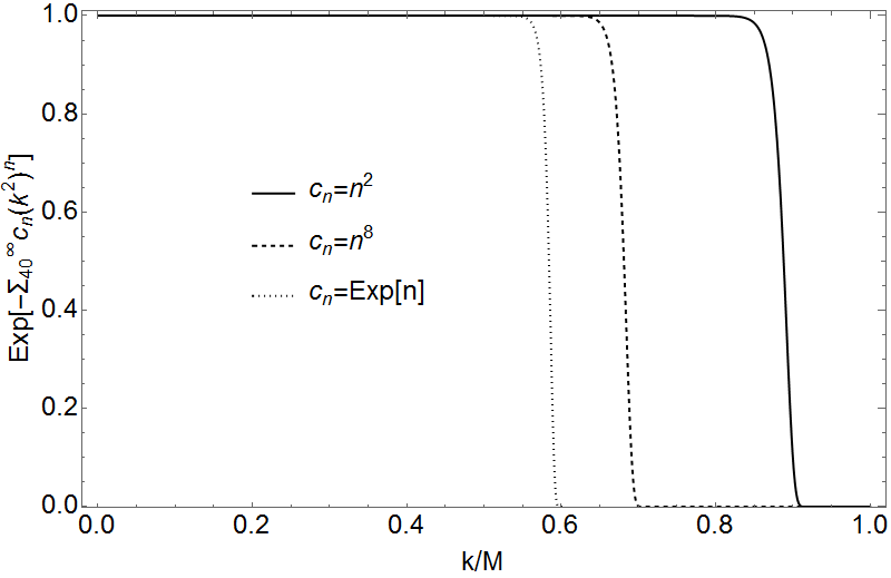
\displaystyle e^{-c_{n}\left(\frac{k^{2}}{M^{2}}\right)^{n}}\approx\text{Rect}\left(\frac{\sqrt[n]{c_{n}}k^{2}}{M^{2}}\right)\equiv\left\{\begin{array}[]{lr}1,&\text{for }\frac{\sqrt[n]{c_{n}}k^{2}}{M^{2}}<1\\ 0,&\text{for }\frac{\sqrt[n]{c_{n}}k^{2}}{M^{2}}>1\end{array}\right\}.

It transpires that when we combine the terms with a large value of $n$ , we can approximate them well as the rectangle function Rect( $Ck^{2}/M^{2}$ ), where $C$ is another constant to be found. This is because an infinite product of rectangle functions

\displaystyle\text{Rect}(a_{1}x)\times\text{Rect}(a_{2}x)\times\cdots,

(3.17)

where $a_{i}>0$ , is equal to the rectangle function given by the lowest value of $a_{i}$ . The validity of this approximation is shown in Fig. 3.1, where we can see that even if $c_{n}$ increases exponentially with $n$ , the approximation is still valid.

3.1.4 Simplest choice of $\gamma(-k^{2})$

For the choice $\gamma=-k^{2}/M^{2}$ , the integral in the function $f(r)$ in (3.11) gives an error function, using

\displaystyle\int_{-\infty}^{\infty}dk\penalty\ e^{-k^{2}/M^{2}}\frac{\sin(kr)}{k}=\pi\text{Erf}\left(\frac{Mr}{2}\right),

(3.18)

which means the potential (3.9) is given by

\displaystyle\Phi(r)=-\frac{2G\mu}{r}\text{Erf}\left(\frac{Mr}{2}\right).

(3.19)

The usual GR potential (3.2) receives a modification in the form of the error function Erf $(r)$ , which is defined as

\displaystyle\text{Erf}(x)=\frac{2}{\sqrt{\pi}}\int^{x}_{0}e^{-t^{2}}dt.

(3.20)

Erf $(r)$ is proportional to $r$ for small $r$ , so (3.19) does not diverge as $r\to 0$ , while Erf $(r)\to 1$ for large $r$ , meaning that $\Phi(r)$ returns to the GR prediction (3.2) at large distances.²² 2 IDG is not the only (metric-tensor based) modified gravity theory to predict a non-singular potential, as higher derivative gravity models can also give finite potentials at the origin (although these models do generically generate ghosts [90, 91]).

By differentiating the potential (3.19), we find the force on a test mass of mass $\mu$ , given by $F(r)=-d\Phi(r)/dr$ [92]

\displaystyle F(r)=-\frac{2G\mu}{r^{2}}\left[\text{Erf}\left(\frac{Mr}{2}\right)-\frac{e^{-\frac{M^{2}r^{2}}{4}}Mr}{\sqrt{\pi}}\right].

(3.21)

It is possible to generalise the potential (3.19) to rotating metrics [93] and charged systems [94].

The avoidance of the singularity at the origin can be related to the non-locality of the action. Non-locality means that interactions no longer take place at a single point but instead are “smeared out” over a wider area, meaning the potential does not diverge at the point where the mass is [75, 29]. This is also how string theory avoids singularities, by replacing point particles with non-local strings [14, 15].

3.1.5 More general choice of $\gamma(-k^{2})$

Monomial choice of $\gamma(-k^{2})$

Next we want to generalise to different choices of $\gamma(-k^{2})$ . The simplest generalisation is to take

\displaystyle\gamma(-k^{2})=-\frac{k^{2n}}{M^{2n}}.

(3.22)

The choice (3.22) gives the general formula [3]³³ 3 (3.23) is a generalisation of [95], which examined only even choices of $n$ in (3.22).

\displaystyle f(r)=\frac{Mr}{n}\sum_{p=0}^{\infty}(-1)^{p}\frac{\Gamma(\frac{p}{n}+\frac{1}{2n})}{(2p+1)!}(Mr)^{2p},

(3.23)

where the Gamma function is $\Gamma(x)\equiv(x-1)!$ .

The plot of $f(r)$ in Fig. 3.2 using (3.23) resembles the error function, but with sinusoidal oscillations that decay in magnitude as we get further away from the source.

Polynomial choice of $\gamma(-k^{2})$

We can generalise even further by using a simple mathematical trick [3]. Any function $\gamma(-k^{2})$ can be written as $\gamma(-k^{2})=-k^{2}/M^{2}-\rho(-k^{2})$ , where $\rho(-k^{2})$ does not contain a term which is quadratic in $k$ . We can expand $e^{\rho(-k^{2})}$ as the infinite sum $e^{\rho(-k^{2})}\equiv\sum^{\infty}_{m=0}\rho_{m}(-1)^{m}k^{2m}/M^{2m}$ , where $\rho_{m}$ are dimensionless coefficients, without any loss of generality. This trick will allow us to utilise the identity (3.18) for more general integrals. We can then write (3.11) as

\displaystyle f(r)=\sum^{\infty}_{m=0}\rho_{m}\int_{-\infty}^{\infty}\frac{dk}{k}\left(\frac{-k^{2}}{M^{2}}\right)^{m}e^{-k^{2}/M^{2}}\sin(kr).

(3.24)

By inserting an auxiliary field $\alpha$ , which we will later set to 1, we can rewrite (3.24) in an advantageous form

\displaystyle f(r)=\sum^{\infty}_{m=0}\rho_{m}\left[\frac{\partial^{m}}{\partial\alpha^{m}}\int_{-\infty}^{\infty}\frac{dk}{k}e^{-\alpha k^{2}/M^{2}}\sin(kr)\right]\bigg|_{\alpha=1}.

(3.25)

Now the integral is just that of (3.18) and thus we simply have

\displaystyle f(r)=\pi\sum^{\infty}_{m=0}\rho_{m}\left[\frac{\partial^{m}}{\partial\alpha^{m}}\text{Erf}\left(\frac{Mr}{2\sqrt{\alpha}}\right)\right]\bigg|_{\alpha=1}.

(3.26)

We can write (3.26) either explicitly as [3]

\displaystyle f(r)=\sum^{\infty}_{m,p=0}\rho_{m}(-1)^{p}\frac{\Gamma(m+p+\frac{1}{2})}{(2p+1)!}\left(Mr\right)^{2p+1},

(3.27)

or using Hermite polynomials $H_{m}(x)\equiv(-1)^{m}e^{x^{2}}\frac{d^{m}}{dx^{m}}e^{-x^{2}}$ as

\displaystyle f(r)=\pi\mathrm{erf}\left(\frac{Mr}{2}\right)-2\sqrt{\pi}e^{-\frac{M^{2}r^{2}}{4}}\sum^{\infty}_{m=1}\rho_{m}(-1)^{m}\frac{1}{4^{m}}H_{2m-1}\left(\frac{Mr}{2}\right)\,.

(3.28)

Clearly, when $\gamma(-k^{2})=-k^{2}/M^{2}$ , therefore $e^{-\rho(-k^{2})}=e^{0}$ and hence $\rho_{0}=1$ and $\rho_{m}=0$ for $m\neq 0$ . Therefore we return to the error function given in (3.18).

Large distance limit

We can check that as $r\to\infty$ , (3.28) converges for any sensible choice of $\tau(-k^{2})$ . For large values of $r$ , we can simplify the second term by noting that $H_{n}(x)=2^{n}x^{n}+O(x^{n-1})$ . Therefore the largest term in $H_{2m-1}\left(\frac{Mr}{2}\right)$ will be $\frac{1}{2}\left(Mr\right)^{2m-1}$ and the second term in (3.28) is proportional to

\displaystyle\lim_{m\to\infty}m!\left(\frac{4}{M^{2}r^{2}}\right)^{m}\rho_{m}(-1)^{m}\frac{1}{4^{m}}\left(Mr\right)^{2m-1}=\lim_{m\to\infty}\rho_{m}(-1)^{m}m!\frac{1}{Mr},

(3.29)

which converges as long as $\rho_{m}$ decreases at least as fast as $\frac{(-1)^{m}}{m!}$ . $\frac{(-1)^{m}}{m!}$ is in fact the $\rho_{m}$ given by the choice $\rho(-k^{2})=-k^{2}$ , and so long as $a(-k^{2})$ fulfils the condition that in the UV limit that the propagator must be suppressed exponentially, i.e. $a(-k^{2})\to\infty$ as $k\to\infty$ , then we will always return to the GR prediction in the IR limit.

As an example, in Fig. 3.3 we plot (3.28) for the binomial choice

\displaystyle\gamma(k^{2})=-\frac{k^{2}}{M^{2}}-a_{N}\frac{k^{2N}}{M^{2N}},

(3.30)

where $a_{N}$ is some dimensionless constant. The choice (3.30) requires our coefficients $\rho_{m}$ to be of the form

\displaystyle\rho_{m}=\frac{(-a_{N})^{m/N}}{(m/N)!}\text{ for }\frac{m}{N}\in\mathbb{N}\text{ and zero otherwise.}

(3.31)

3.1.6 Comparison to experiment

Constraining the error function potential

Using the equipment shown in Fig. 3.4, Adelberger [4] found that the $1/r$ fall of the potential continued down to $5.6\times 10^{-5}$ m. The experiment assumed that any modification to GR would be a Yukawa potential of the form

\displaystyle V(r)=\frac{V_{0}}{r}\left[1+\exp(-r/\lambda)\right],

(3.32)

and ruled out the potential (3.32) with $\lambda>5.6\times 10^{-5}$ m. By seeing the value of $M$ for which our potential gives a bigger divergence from GR than the Yukawa potential, we see where our potential would be ruled out. Taking $\gamma=-k^{2n}$ , and using equation (3.23), we found a constraint of $M>$ 0.004, 0.02, 0.03, 0.05 eV for $n=$ 1, 2, 4, 8 respectively.

Constraining the oscillating potential

We know that higher powers of $n$ give an oscillating function for $r>M^{-1}$ , but work by Perivolaropoulos [5] showed that for $n>10$ one can accurately parameterise (3.23) as

	$\displaystyle f(r)$	$\displaystyle=$	$\displaystyle\alpha_{1}Mr,\quad\quad\penalty\ \penalty\ \penalty\ \penalty\ \penalty\ \penalty\ \penalty\ \penalty\ \penalty\ \penalty\ \penalty\ \penalty\ 0<Mr<1$
	$\displaystyle f(r)$	$\displaystyle=$	$\displaystyle 1+\alpha_{2}\frac{\cos(Mr+\theta)}{Mr},\quad\quad Mr>1$		(3.33)

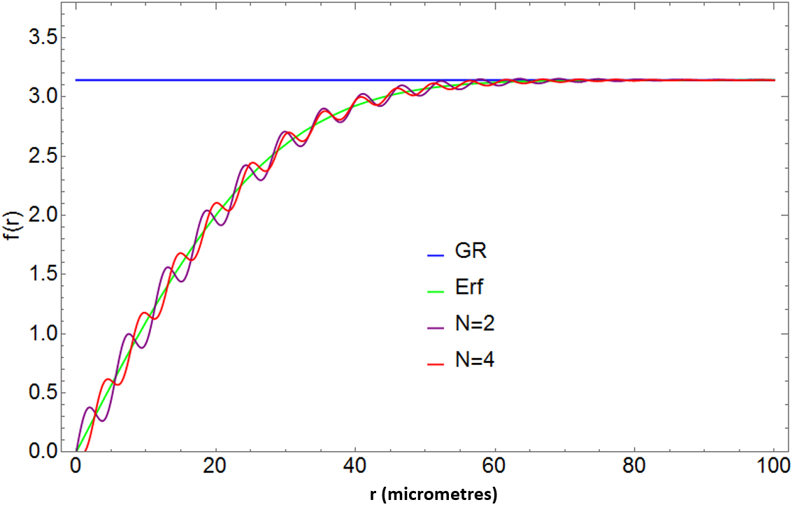
where $\alpha_{1}=0.544$ , $\alpha_{2}=0.572$ , $\theta=0.855\hskip 2.27621pt\pi$ . This parameterisation is a good approximation because for high $n$ , $\exp(-ax^{n})$ forms a rectangle function as shown in (3.1.3).

The best fit of (3.1.6) actually provides a better fit to the data from the Adelberger experiment than the standard $1/r$ fall of the potential that GR predicts by around 2 $\sigma$ [5]. Perivolaropoulos’ results are plotted in Fig. 3.5. While the better fit than GR could be a case of fine-tuning, it certainly gives experimentalists an impetus to look for other modified gravity theories when they undertake tests of gravity at short distances. Currently they largely test only for either a Yukawa potential or GR.

3.2 $a\neq c$

While investigating the Newtonian potential, we have so far taken the choice $a=c$ . However, this case doesn’t allow defocusing of null rays [87], as we will later see in Section 4.3, and therefore leads to geometric singularities through the Hawking-Penrose singularity theorems [24]. We therefore should investigate what happens to the potential when we take $a\neq c$ by using (2.40) from earlier. This fulfils the defocusing conditions which we later find in Section 4.3, and as we will later see, provides a similar prediction for the potential at high $n$ .

Taking the choice of $c(\Box)$ given in (2.40), then (3.10) becomes

\displaystyle f(r)=\int^{\infty}_{-\infty}dk\left[4-\frac{m^{2}}{\tilde{a}(-k^{2})(m^{2}+k^{2})}\right]\frac{\sin(kr)}{k\penalty\ a(-k^{2})}.

(3.34)

We recall that we require both $a(-k^{2})$ and $\tilde{a}(-k^{2})$ to be the exponential of entire functions so that no ghosts are generated, i.e. $a(-k^{2})=e^{\gamma(-k^{2})}$ and $\tilde{a}(-k^{2})=e^{\tau(-k^{2})}$ . Therefore (3.34) becomes [6]

\displaystyle f(r)=\int^{\infty}_{-\infty}dk\left[4-\frac{m^{2}}{(m^{2}+k^{2})e^{\tau(-k^{2})}}\right]\frac{e^{-\gamma(-k^{2})}\sin(kr)}{k}.

(3.35)

Conditions on $\gamma(-k^{2})$ and $\tau(-k^{2})$

By considering the behaviour of the propagator (2.42), we can find conditions on $\gamma(-k^{2})$ and $\tau(-k^{2})$ . In the ultraviolet regime, we want the propagator to be exponentially suppressed. The coefficient of the $P^{2}$ component is $e^{-\gamma(-k^{2})}$ and therefore we require that $\gamma(k^{2})>0$ (and that $\gamma$ is not a constant). Similarly the coefficient of the $P^{0}_{s}$ component is $e^{-\left(\gamma(-k^{2})+\tau(-k^{2})\right)}$ and therefore we require $\gamma(-k^{2})+\tau(-k^{2})>0$ . The defocusing condition for a static perturbation is found in Section 4.3.2 and is given by [87]

\displaystyle\left(1-\Box/m^{2}\right)\tilde{a}(\Box)r>r,

(3.36)

where $r$ is the perturbed Ricci scalar. Given our earlier choice $\tilde{a}(-k^{2})=e^{\tau(-k^{2})}$ , we see that moving to momentum space gives

\displaystyle\left(1+k^{2}/m^{2}\right)e^{\tau(-k^{2})}\hskip 1.42262pt\tilde{r}>\tilde{r}.

(3.37)

where $\tilde{r}$ is the Fourier transform of $r$ . If (3.37) holds true for all $k$ , then we have the condition that $\tau(-k^{2})\geq 0$ . The result of these three constraints is that the integral (3.35) converges.

We now have two undetermined entire functions $\tau(-k^{2})$ and $\gamma(-k^{2})$ and two free mass scales. We will choose both our mass scales to be the Planck mass $M_{P}$ and take $\tau(-k^{2})=0$ , so that all the model freedom is in the function $\gamma(-k^{2})$ . The simplest choice for $\gamma$ is the monomial $\gamma(-k^{2})=(Ck^{2}/M^{2}_{P})^{D}$ . We now have only two free parameters, $C$ and $D$ , and our integral becomes [6]

\displaystyle f(r)=\int^{\infty}_{-\infty}dk\left[4-\frac{M^{2}_{P}}{(M^{2}_{P}+k^{2})}\right]\frac{e^{-(Ck^{2}/M^{2}_{P})^{D}}\sin(kr)}{k}.

(3.38)

While this choice is fairly restrictive, we obtain qualitatively similar results for other choices of the mass scales and the function $\tau(-k^{2})$ .

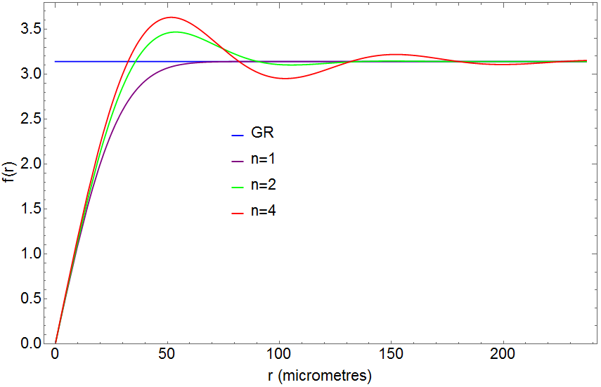
We first take the case $D=1$ and plot (3.38) in Fig. 3.6 for different values of $C$ [6]. We can see that increasing $C$ makes the IDG effect stronger at distances further away from the source. This effect is akin to decreasing the mass scale $M$ for the $a=c$ case.

In Fig. 3.7, we take $C=1$ and plot $f(r)$ for different $D$ [6]. As for the $a=c$ case, we find oscillations for $D>1$ which have approximately constant frequency and decaying amplitude as $r$ increases. To being with, these oscillations become larger in amplitude as we increase $D$ , but this effect stops for around $D>10$ because at this point (3.1.3) becomes a good approximation and so increasing $D$ further has no effect on the amplitude of the oscillations.

We also show in the plot Fig. 3.8 that we can accurately approximate the potential⁴⁴ 4 In this plot, we obtain a slightly better match to (3.38) by changing from the first to the second case in (3.1.6) at $Mr=2.2$ rather than 1. with the parameterisation (3.1.6) which matches the experimental results [6].

Figure 3.8: We show that the black line, representing (3.1.6) is a valid approximation to the green, blue and red coloured dots, representing

D

=11, 12, 13 in (3.38) respectively [6]. We have chosen

\alpha_{1}=0.388

\alpha_{2}=0.6

and

\theta=2.75

3.3 Raytracing

In Appendix A.4 we give the method for calculating the trajectory of photons passing a point mass of mass $m$ in GR against IDG. By making a coordinate transform, one can write the metric (3.1) with the potential (3.19) as

\displaystyle d\tau^{2}=\left(1-\frac{r_{*}}{r}\text{Erf}\left(\frac{Mr}{2}\right)\right)dt^{2}-\left(1-\frac{r_{*}}{r}\text{Erf}\left(\frac{Mr}{2}\right)\right)^{-1}dr^{2}-r^{2}d\phi^{2}.

(3.39)

One finds that the path of the photons can be described by

\displaystyle u^{\prime\prime}(\phi)=-u(\phi)+\frac{3}{2}r_{*}u^{2}(\phi)\text{Erf}\left(\frac{M}{2u(\phi)}\right)+\frac{r_{*}u^{3}(\phi)}{2}\text{Erf}^{\prime}\left(\frac{M}{2u(\phi)}\right),

(3.40)

where we have defined $u\equiv 1/r$ , $r_{*}=2Gm$ and the primes represent differentiation with respect to $\phi$ . In Fig. 3.9 we plot various photon trajectories to see the effect IDG has on the photon trajectory in GR.

One can see that the photons are more strongly attracted to the mass in GR than in IDG, especially when they are closer to the mass.

3.4 Potential around a de Sitter background

We could use the de Sitter background as written in (2.15). However, if we perturb (2.15) with a point source which generates a potential $\Phi(r)$ , we will have an arbitrarily large number of d’Alembertian operators acting on functions of both $r$ and $t$ , which is non-trivial to solve.

However, we can write the de Sitter metric so that its coefficients have no time dependence, whilst retaining the same equations of motion and the maximal symmetry [96]. The perturbed de Sitter background can then be written as

\displaystyle ds^{2}=-\left(1+2\Phi(r)-H^{2}r^{2}\right)dt^{2}+\left(1-2\Psi(r)\right)\left[\left(1+H^{2}r^{2}\right)dr^{2}+r^{2}d\Omega^{2}\right],\penalty\ \penalty\

(3.41)

where we are working in the regime $H^{2}r^{2}\ll 1$ to simplify the ensuing analysis [97]. This is justified because we are interested in probing IDG at very short distances from the object producing the potential compared to the size of the cosmological horizon.

In this approximation, the background de Sitter d’Alembertian operator $\bar{\Box}$ acting on a function of $r$ takes on a pleasing form

$\displaystyle\bar{\Box}X(r)$	$\displaystyle=$	$\displaystyle\bigg[\frac{1}{1+H^{2}r^{2}}\partial_{r}-\frac{H^{2}r}{1+H^{2}r^{2}}\left(\frac{1}{1-H^{2}r^{2}}+\frac{1}{1+H^{2}r^{2}}\right)+\frac{2}{r}\frac{1}{1+H^{2}r^{2}}\bigg]\partial_{r}X(r)$	(3.42)
	$\displaystyle\approx$	$\displaystyle\left(\partial_{r}^{2}+\frac{2}{r}\partial_{r}\right)X(r)$
	$\displaystyle=$	$\displaystyle\Delta X(r),$

where we have defined $\Delta\equiv\eta^{ij}\nabla_{i}\nabla_{j}$ as the Laplace operator for a flat background.

We will need the following perturbed Ricci curvatures for the metric (3.41) up to linear order in $\Phi$ and $\Psi$ (and their derivatives).

$\displaystyle R_{tt}$	$\displaystyle\approx$	$\displaystyle\Delta\Phi(r)-3H^{2}\left(1+2\Psi(r)-\Phi(r)\right),$
$\displaystyle R_{rr}$	$\displaystyle\approx$	$\displaystyle\frac{2\left(r\Psi^{\prime\prime}(r)+\Psi^{\prime}(r)\right)}{r}-\Phi^{\prime\prime}(r)+H^{2}\bigg[3-r\Phi^{\prime}(r)-2\Phi(r)+4\Psi(r)\bigg],$
$\displaystyle R$	$\displaystyle\approx$	$\displaystyle 4\Delta\Psi(r)-2\Delta\Phi(r)+12H^{2}\left(1+3\Psi(r)-\Phi(r)\right).\penalty\ \penalty\ \penalty\$	(3.43)

By substituting the perturbed Ricci curvatures into the equations of motion (2.26), we find that

\displaystyle\hskip-6.54413pt\frac{\Psi(r)}{\Phi(r)}\hskip-1.99168pt=\hskip-1.99168pt\frac{a(\Delta)(\Delta+3H^{2})-\left(3c(\Delta)+\Delta f(\Delta)\right)\left(\Delta+6H^{2}\right)}{a(\Delta)(4\Delta+30H^{2})-2\left(3c(\Delta)+\Delta f(\Delta)\right)\left(\Delta+9H^{2}\right)},\penalty\ \penalty\ \penalty\ \penalty\ \penalty\ \penalty\

(3.44)

and we can find $\Phi$ in terms of the density $\rho$ of our source

\displaystyle\left(\Delta^{2}+15H^{2}\Delta+63H^{4}\right)\Phi(r)=\frac{\rho}{M^{2}_{P}}\frac{a(\Delta)(2\Delta+15H^{2})-\left(3c(\Delta)+\Delta f(\Delta)\right)\left(\Delta+9H^{2}\right)}{a(\Delta)\left[2a(\Delta)-4c(\Delta)-\Delta f(\Delta)\right]}.\hskip 1.13809pt\penalty\ \penalty\ \penalty\ \penalty\ \penalty\

(3.45)

The energy density of a point source of mass $\mu$ is $\rho=\mu\hskip 2.27621pt\delta^{3}(\textbf{x})$ . We again go into momentum space in order to write $\Phi(r)$ as an integral

	$\displaystyle\Phi(r)=\frac{\mu}{2\pi^{2}M^{2}_{P}r}I(k)$
	$\displaystyle\hskip 27.17238pt=\frac{\mu}{2\pi^{2}M^{2}_{P}r}$
	$\displaystyle\cdot\int^{\infty}_{-\infty}dk\penalty\ k\sin(kr)\frac{a(-k^{2})(15H^{2}-2k^{2})+\left(3c(-k^{2})-k^{2}f(-k^{2})\right)\left(k^{2}+9H^{2}\right)}{a(-k^{2})\left(2a(-k^{2})-4c(-k^{2})+k^{2}f(-k^{2})\right)\left(k^{4}-15H^{2}k^{2}+63H^{4}\right)}.\penalty\ \penalty\ \penalty\ \penalty\ \penalty\ \penalty\ \penalty\ \penalty\ \penalty\$		(3.46)

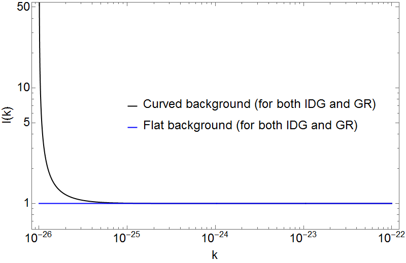
We note that the current value of the Hubble parameter, $H=7.25\times$ $10^{-27}$ m^-1 is many orders of magnitude smaller than even the lower bound on the mass scale of IDG [3], $M=1.79\times 10^{4}$ m^-1. At current times, i.e. when we conduct experiments on the potential generated by IDG, we can therefore ignore the background curvature, as detailed further in Fig. 3.10 and Fig. 3.11, and use our results from Section 3.1.

3.5 Summary

In this chapter we investigated the Newtonian potential, which is the potential generated by a point mass in a background. We first found the potential around a Minkowski background for various choices of the form of the propagator assuming that it had no poles. Regardless of the choice made, we always generate a non-singular potential that returns to GR at large distances. For certain choices, we obtained an oscillating potential. Using our results, it was found that the oscillating potential could provide a better fit to experimental data than GR [5].

We further showed that if the propagator has a single pole, it still generates a non-singular potential which returns to GR at large distances and can produce an oscillating potential. We generalised our method to a de Sitter background and found that the low value of the Hubble parameter today means that it makes a negligible difference to the potential and we can safely use the calculation from a flat background.

Chapter 4 Defocusing and geodesic completeness

4.1 Notion of a singularity

A singularity is traditionally defined as a place where the curvature blows up, i.e. becomes infinite [98]. In other theories, a singular potential is a relatively easy concept to understand. In electromagnetism, the Coulomb potential is infinite in various scenarios, for example the potential given by a point charge diverges at the point itself. The issue with extending the idea of a singular potential to GR is that we need to solve for the metric of spacetime itself. If the metric potential diverges, then we do not have a complete description of spacetime and it is difficult to understand what a “place” means in our definition of a singularity. In other words, if we cannot define the manifold, we cannot say where the “place” is that the curvature diverges.

Geodesic completeness

The solution to our dilemma lies in the idea of geodesic past-completeness. In a non-singular spacetime, one can take a geodesic and trace its path back to null past infinity. The property of being able to trace the path back is the definition of geodesic completeness, which we will later use to find the conditions for IDG to avoid the singularities produced in GR.

One can imagine a spacetime with ‘holes’ in its fabric, defined by geodesics being unable to traverse them, and which would thus be geodesically incomplete [29]. A particle which is falling freely in such a spacetime would cease to exist at a finite proper time. It must be mentioned that the definition of geodesic completeness is not as precise as we would perhaps wish. It is possible for our imaginary spacetime to be geodesically incomplete for spacelike or timelike vector fields and still be geodesically complete for the other two ¹¹ 1 In full, a spacetime can be geodesically incomplete for spacelike vector fields while still complete for timelike and null vector fields, or could be incomplete for timelike vector fields while incomplete for spacelike and null vector fields. Further details of the possible permutations are given in [99]. [29]. However, it is clear that if a spacetime is geodesically incomplete for null or timelike fields, then we will not be able to fully describe the spacetime geometry. The definition of geodesic incompleteness to be used in this chapter is based on the Hawking-Penrose singularity theorems, which tell us whether a spacetime will be geodesically complete.

4.2 Raychaudhuri equation

The Raychaudhuri equation is a geometric equation which is model-independent in that it depends on gravity only through its effect on the curvature of spacetime [98, 54].

If there exists a congruence of null rays, then the tangent vectors to the congruence $k_{\mu}$ satisfy $k^{\mu}k_{\mu}=0$ . These are defined through $k^{\mu}\equiv\frac{dx^{\mu}}{d\lambda}$ where $\lambda$ is an affine parameter [98, 54].

We can define several parameters of the congruence using these tangent vectors. The expansion $\theta$ , shear $\sigma_{\mu\nu}$ and rotation/twist $\omega_{\mu\nu}$ are

\displaystyle\theta\equiv\nabla^{\mu}k_{\mu},\quad\sigma_{\mu\nu}=\nabla_{(\mu}k_{\nu)},\quad\omega_{\mu\nu}=\nabla_{\mu}k_{\nu}-\nabla_{\nu}k_{\mu}.

(4.1)

The Raychaudhuri equation for null geodesic congruences is

\displaystyle\frac{d\theta}{d\lambda}+\frac{1}{2}\theta^{2}=-\sigma_{\mu\nu}\sigma^{\mu\nu}+\omega_{\mu\nu}\omega^{\mu\nu}-R_{\mu\nu}k^{\mu}k^{\nu},

(4.2)

using $k^{\lambda}\nabla_{\lambda}\theta=\frac{d\theta}{d\lambda}$ . The Hawking-Penrose singularity theorem states that unless $\theta$ is both positive and increasing, a singularity will be generated [24]. By choosing the congruence wisely²² 2 Strictly speaking the congruence of null rays must be orthogonal to a hypersurface., we can discard the twist tensor term and we can note that the shear tensor is purely spatial and so $\sigma_{\mu\nu}\sigma^{\mu\nu}$ is non-negative.

This leads us to the null convergence condition (null CC)

\displaystyle\frac{d\theta}{d\lambda}+\frac{1}{2}\theta^{2}\leq-R_{\mu\nu}k^{\mu}k^{\nu}.

(4.3)

If this is fulfilled, singularities are generated. The absolute minimum necessary condition to avoid these singularities, known as the minimum defocusing condition is

\displaystyle R_{\mu\nu}k^{\mu}k^{\nu}<0.

(4.4)

The Null Energy Condition (NEC) means that in GR, (4.4) cannot be satisfied and so singularities are generated. The NEC states that the stress-energy tensor contracted with the tangent vectors is positive, i.e. $T_{\mu\nu}k^{\mu}k^{\nu}\geq 0$ . By inserting the Einstein equation (1.2) into (4.4), it can be seen that the defocusing condition will not be satisfied in GR as long as the NEC holds, i.e. as long as we do not introduce exotic matter which violates the NEC. However in IDG, it is possible to satisfy the defocusing condition due to our modification to the Einstein equation.

4.3 Defocusing around a flat background

We now examine the necessary condition for defocusing for perturbations around a flat background, in the context of singularity avoidance, especially in the early universe. We contract the linearised equations of motion around a flat background (2.11) with $k^{\mu}k^{\nu}$ to give the defocusing condition [87]

\displaystyle k^{\mu}k^{\nu}r_{\mu\nu}=\frac{1}{a(\Box)}\left(M^{-1}_{P}T_{\mu\nu}k^{\mu}k^{\nu}+\frac{1}{2}k^{\mu}k^{\nu}f(\Box)\nabla_{\mu}\nabla_{\nu}r\right)<0.

(4.5)

where $r_{\mu\nu}$ and $r$ are the perturbed Ricci tensor and perturbed Ricci scalar respectively. As in Section 2.2.3, we require $a(-k^{2})>0$ to avoid a Weyl ghost [79, 76, 29]. Due to the Null Energy Condition (NEC) $T_{\mu\nu}k^{\mu}k^{\nu}\geq 0$ , the minimum condition to avoid a singularity is therefore

\displaystyle k^{\mu}k^{\nu}f(\Box)\nabla_{\mu}\nabla_{\nu}r<0.

(4.6)

4.3.1 Homogenous perturbation

We examine the case where the perturbed curvature depends only on the cosmic time $t$ . This is useful for considering cosmological singularities by using a perturbation around a Minkowski background as an approximation to the FRW metric (4.30). Using $\Box r(t)=-\partial_{t}^{2}r(t)$ for a flat background, (4.6) simplifies to

\displaystyle\left(k^{0}\right)^{2}f(\Box)\Box r(t)>0,

(4.7)

and using $f(\Box)\Box=a(\Box)-c(\Box)$ from (2.2.1), (4.7) becomes

\displaystyle\left(a(\Box)-c(\Box)\right)r(t)>0

(4.8)

The simple choice $a(\Box)=c(\Box)$ does not allow defocusing [87]. We can make a choice of $a(\Box)\neq c(\Box)$ , but this choice introduces an extra pole in the propagator, which in theory could produce a ghost.³³ 3 We could choose $a=Ac=e^{\gamma(k^{2})}$ where $A$ is a constant, but if we want to return to GR in the low energy limit then we are forced to choose $A=1$ . However, we showed in Section 2.2.3 that a single extra pole was allowed and we introduced the choice (2.40) which generates one extra pole in the propagator.

With the choice (2.40), the defocusing condition becomes

\displaystyle\left(1-\Box/m^{2}\right)\tilde{a}(\Box)r<r.

(4.9)

4.3.2 Static perturbation

We next examine the case where the perturbation is a function only of a single spatial coordinate $x$ . In this case, the defocusing condition (4.6) is

\displaystyle k^{i}k^{j}f(\Box)\partial_{i}\partial_{j}\hskip 1.13809ptr(x)<0.

(4.10)

Using (2.2.1) and $\Box r(x)=\partial_{i}^{2}r(x)$ , we find the minimum defocusing condition

\displaystyle\left(a(\Box)-c(\Box)\right)r(x)<0.

(4.11)

Note the change of sign from the homogenous case (4.8). Once again, $a(\Box)=c(\Box)$ does not allow defocusing so we take the choice (2.40) giving [6]

\displaystyle\left(1-\Box/m^{2}\right)\tilde{a}(\Box)r>r.

(4.12)

This is the condition we used to derive (3.37).

4.3.3 Inhomogenous perturbations

Lastly we examine perturbations which are functions of time and a single Cartesian coordinate, which we take to be $x$ here. The defocusing condition (4.6) becomes

\displaystyle\left((k^{0})^{2}f(\Box)\partial_{t}^{2}+(k^{x})^{2}f(\Box)\partial_{x}^{2}\right)r(t,x)<0

(4.13)

From the condition $g_{\mu\nu}k^{\mu}k^{\nu}=0$ (i.e. the requirement that the vector $k_{\mu}$ is null), we deduce that $(k^{0})^{2}=(k^{x})^{2}$ , so noting that $(k^{0})^{2}$ is strictly positive and assuming that the stress energy tensor is a perfect fluid⁴⁴ 4 If $T_{\mu\nu}$ is a perfect fluid, it has no off-diagonal terms and therefore there are no cross terms in (4.5).,

\displaystyle f(\Box)\left(\partial_{t}^{2}+\partial_{i}^{2}\right)r(t,x_{i})<0.

(4.14)

4.4 Defocusing around backgrounds expanding at a constant rate

4.4.1 (Anti) de Sitter

Around a curved (Anti) de Sitter background, the linear equations of motion become more complicated but are nonetheless tractable. Contracting the equations of motion (2.26) with the tangent vectors $k_{\mu}k^{\nu}$ , and the defocusing condition becomes

\displaystyle r^{\mu}_{\nu}k_{\mu}k^{\nu}=\frac{1}{a(\Box)}\left[M^{-2}_{P}T^{\mu}_{\nu}k_{\mu}k^{\nu}+\frac{1}{2}k_{\mu}k^{\nu}\nabla^{\mu}\partial_{\nu}f(\Box)r\right]<0,

(4.15)

where $r$ is the perturbed Ricci tensor. We already know that $T^{\mu}_{\nu}k_{\mu}k^{\nu}$ must be positive by the NEC (as long as we have non-exotic matter) and that (in momentum space) $a(-k^{2})$ must be positive, otherwise the background de Sitter spacetime will have a negative entropy [48, 29]. (4.15) can then be simplified to give the minimum defocusing condition [100]

\displaystyle k_{\mu}k^{\nu}\nabla^{\mu}\partial_{\nu}f(\Box)r<0.

(4.16)

If the perturbation is homogenous, i.e. $r=r(t)$ , then we can expand the covariant derivatives and note that the d’Alembertian acting on a scalar function of time is $\Box=-\partial_{t}^{2}-3H\partial_{t}$ , so (4.16) becomes

\displaystyle\Box f(\Box)r(t)>-4H\partial_{t}f(\Box)r(t).

(4.17)

4.4.2 Anisotropic backgrounds

AdS-Bianchi I metric

We now look at anisotropic backgrounds. The observable universe is almost exactly isotropic (looks the same in different spatial directions) [98], but it is interesting to consider anisotropy. This is because while the anisotropy in the observable universe is very small, it is unlikely to be exactly zero so we should consider its effects. Furthermore, just because our observable universe is isotropic does not mean the rest of the universe is as well. We study the anisotropic metric

\displaystyle ds^{2}=-dt^{2}+e^{2At}dx^{2}+e^{2Bt}dy^{2}+e^{2Ct}dz^{2},

(4.18)

where $A$ , $B$ , and $C$ are positive constants, which we call an (A)dS-Bianchi I metric. The observable universe is highly isotropic [98], so we assume that $A$ , $B$ , and $C$ are almost equal.

The (A)dS-Bianchi I metric (4.18) produces a constant background Ricci tensor $\bar{R}_{\mu\nu}$ and a constant positive Ricci scalar $\bar{R}=2\left(A^{2}+B^{2}+C^{2}+AB+AC+BC\right)$ .

Equations of motion

Studying the reduced action ⁵⁵ 5 We have set $F_{2}(\Box)=F_{3}(\Box)=0$ to simplify our calculations.

\displaystyle S=\frac{1}{16\pi G}\int d^{4}x\,\sqrt{-g}\left[R+R\mathcal{F}(\Box)R\right],

(4.19)

around the background (4.18) gives the equations of motion

\displaystyle T^{\alpha}_{\beta}=\left(M^{2}_{p}+2f_{0}\bar{R}\right)\left(r^{\alpha}_{\beta}-\frac{1}{2}\delta^{\alpha}_{\beta}r\right)+\left(2\bar{S}^{\alpha}_{\beta}+\frac{1}{2}\delta^{\alpha}_{\beta}\bar{R}-2\nabla^{\alpha}\nabla_{\beta}+2\delta^{\alpha}_{\beta}\Box\right)F(\Box)r.\penalty\ \penalty\ \penalty\ \penalty\

(4.20)

These are the same as the (A)dS field equations for the action (4.19) apart from the additional term with the traceless curvature tensor $\bar{S}^{\alpha}_{\beta}\equiv\bar{R}^{\alpha}_{\beta}-\frac{1}{4}\delta^{\alpha}_{\beta}\bar{R}$ .

To find the necessary conditions to avoid singularities, we use the same method as in Section 4.3, contracting (4.20) with $k^{\beta}k_{\alpha}$ to give the defocusing condition for a generic null tangent vector $k^{\alpha}$ [100]

\displaystyle k^{\beta}k_{\alpha}r^{\alpha}_{\beta}=\frac{1}{M^{2}_{P}+2f_{0}\bar{R}}\bigg(k^{\beta}k_{\alpha}T^{\alpha}_{\beta}-2\lambda k^{\beta}k_{\alpha}\bar{R}^{\alpha}_{\beta}F(\Box)r+2\lambda k^{\beta}k_{\alpha}\nabla^{\alpha}\nabla_{\beta}F(\Box)r\bigg)<0.\penalty\ \penalty\ \penalty\ \penalty\

(4.21)

Choice of $k_{\alpha}$

Thus far we have not had to choose $k_{\alpha}$ , because the condition $k^{\alpha}k_{\alpha}=0$ and the isometry of the Minkowski and (Anti) de Sitter background has ensured that we can easily find $(k^{0})^{2}$ in terms of $(k^{i})^{2}$ . However, that is no longer true when we introduce anisotropy. We therefore have to choose $k^{\alpha}$ carefully. We must both satisfy the geodesic equations and ensure that the rotation term vanishes.

If $k_{\mu}$ is of the form, $k_{\mu}=(k_{0},k_{x},0,0)$ , the non-trivial geodesic equations for the null ray are

\displaystyle\frac{d^{2}t}{d\lambda^{2}}+Ae^{2At}\hskip 1.13809pt\frac{dx}{d\lambda}\frac{dx}{d\lambda}=0,\quad\quad\frac{d^{2}x}{d\lambda^{2}}+2A\hskip 0.56905pt\frac{dx}{d\lambda}\frac{dt}{d\lambda}=0,

(4.22)

where $\lambda$ is the affine parameter. By dividing $g_{\mu\nu}dx^{\mu}dx^{\nu}=0$ (the condition for the vector $k_{\mu}\equiv\frac{dx_{\mu}}{d\lambda}$ to be null) by $d\lambda^{2}$ , we see that

\displaystyle\frac{dt}{d\lambda}=e^{At}\frac{dx}{d\lambda}.

(4.23)

Combining (4.22) and (4.23) leads to

\displaystyle\frac{dt}{d\lambda}=k^{0}=Ce^{-At},\quad\quad\frac{dx}{d\lambda}=k^{x}=e^{-2At}.

(4.24)

For simplicity we choose $C=1$ to give

\displaystyle k_{\mu}=(-e^{-At},1,0,0).

(4.25)

For the rotation term to vanish, we require [54]⁶⁶ 6 The Christoffel symbols generated by the covariant derivatives in (4.26) cancel out due to the symmetry in the lower indices of the Christoffel symbol, so that only partial derivatives remain.

\displaystyle\omega_{\alpha\beta}\equiv\nabla_{\alpha}k_{\beta}-\nabla_{\beta}k_{\alpha},

(4.26)

to be zero, which is satisfied by (4.25). If we assume the perturbation depends only on time, then our defocusing condition becomes (using the NEC) [100]⁷⁷ 7 We assume here that $f_{0}$ is positive, as we later use IDG as an extension to Starobinsky $R+R^{2}$ inflation. We also note that $\bar{R}$ is non-negative.

\displaystyle\bigg[\partial_{t}^{2}-A\partial_{t}+(B^{2}+C^{2})-A(B+C)\bigg]F(\Box)r(t)<0,

(4.27)

How does (4.27) compare with the (A)dS case (4.16)? If we take $H=A$ , then we can see that the addition of anisotropy has generated an additional term

\left[B^{2}+C^{2}-A(B+C)\right]F(\Box)r(t).

(4.28)

Thus anisotropy can have a significant effect on whether a spacetime can avoid the null CC condition (4.3), especially for slowly evolving perturbations, and therefore whether the spacetime will generate singularities.

4.5 Defocusing in more general spacetimes

4.5.1 A constraint on the curvature adapted to IDG

Even for the reduced action⁸⁸ 8 More generally there are more terms, but for an FRW metric with spatial curvature $\kappa=0$ , the Weyl tensor is zero and we can discard the Ricci tensor term using the extended Gauss-Bonnet identity [80].,

	$\displaystyle S$	$\displaystyle=$	$\displaystyle\frac{1}{16\pi G}\int d^{4}x\,\sqrt{-g}\left[R+R\mathcal{F}(\Box)R-2\Lambda\right],$		(4.29)
			$\displaystyle\text{where }\mathcal{F}(\Box)=\sum_{n=0}^{\infty}f_{n}\left(\frac{\Box}{M^{2}}\right)^{n},$		(4.29)

it is almost impossible to solve the equations of motion for IDG for the more general Friedmann-Robertson-Walker (FRW) metric

\displaystyle ds^{2}=-dt^{2}+\frac{a^{2}(t)}{1-\kappa r^{2}}\left(dx^{2}+dy^{2}+dz^{2}\right)

(4.30)

where $a(t)$ is the scale factor of the universe and $\kappa$ is the spatial curvature.

The FRW metric has the Christoffel symbols

\displaystyle\Gamma^{t}_{ij}=a^{2}H\delta_{ij},\quad\quad\Gamma^{i}_{tj}=H\delta^{i}_{j},

(4.31)

where $\delta_{ij}$ is the Kronecker delta function, which is 1 if $i=j$ and zero otherwise. By using an ansatz we can simplify the equations of motion [33], to make it possible to generate a solution for the scale factor. We choose the ansatz

\displaystyle\Box R=r_{1}R+r_{2},

(4.32)

where $r_{1}$ and $r_{2}$ are constants, which means that for $n>0$ , $\Box^{n}R=r_{1}^{n}\left(R+\frac{r_{2}}{r_{1}}\right)$ . Using this ansatz, it is possible to show that $a(t)=\cosh(\sigma t)$ and $a(t)=e^{\lambda t^{2}}$ are solutions to the IDG equations of motion for the action, where $\sigma$ and $\lambda$ are constants [33, 101, 102, 103, 104]. It is notable that both these scale factors generate bouncing universes, meaning that at some scale, gravity becomes repulsive such that the universe is forced to stop contracting and start expanding.

In this section we will test whether such bouncing solutions can avoid the Hawking-Penrose singularity within the IDG framework and are thus geodesically complete. While one might expect that any FRW spacetime with a non-singular metric would be geodesically complete, this is not necessarily the case [105, 106, 107].

Here we will focus on FRW spacetimes, but one should note (as found by Sravan Kumar⁹⁹ 9 This work is so far unpublished.) that anisotropic metrics of the form

\displaystyle ds^{2}=-dt^{2}+e^{2\sigma t^{2}}dx^{2}+e^{2\gamma t^{2}}\left(dy^{2}+dz^{2}\right),

(4.33)

where $\sigma$ and $\gamma$ are positive constants, would also fulfil the ansatz (4.32) which could be a topic of further study.

4.5.2 Defocusing with the ansatz

By contracting the equations of motion for the action (4.29) with $k^{\mu}k^{\nu}$ , the defocusing condition (4.4) for any general metric is

	$\displaystyle k^{\alpha}k^{\beta}R_{\alpha\beta}$	$\displaystyle=$	$\displaystyle\frac{1}{M^{2}_{p}+4F(\Box)R}\bigg[k^{\beta}k^{\alpha}T_{\alpha\beta}+4k^{\beta}k^{\alpha}\nabla_{\alpha}\nabla_{\beta}F(\Box)R$		(4.34)
			$\displaystyle+2k^{\beta}k^{\alpha}\sum^{\infty}_{n=1}\frac{f_{n}}{M^{2n}}\sum^{n-1}_{l=0}\left(\partial_{\alpha}\Box^{l}R\right)\partial_{\beta}\Box^{n-l-1}R\bigg]<0.$		(4.34)

Using the ansatz (4.32), (4.34) becomes

	$\displaystyle\frac{1}{M^{2}_{p}+4F(r_{1})\left(R+\frac{r_{2}}{r_{1}}\right)-4f_{0}r_{2}/r_{1}}\bigg[k^{\beta}k^{\alpha}T_{\alpha\beta}+4k^{\beta}k^{\alpha}\sum_{n=0}^{\infty}\frac{f_{n}}{M^{2n}}\nabla_{\alpha}\nabla_{\beta}\left(r^{n}_{1}R\right)$
	$\displaystyle+2k^{\beta}k^{\alpha}\sum^{\infty}_{n=1}\frac{f_{n}}{M^{2n}}\sum^{n-1}_{l=0}\partial_{\alpha}\left(r^{l}_{1}R\right)\partial_{\beta}\left(r_{1}^{n-l-1}R\right)\bigg]<0.$		(4.35)

We note that $r_{1}$ is a constant so we can pull these terms out of the derivatives, which means the last term depends on

\displaystyle\sum^{n-1}_{l=0}\left(\partial_{\alpha}R\right)\left(\partial_{\beta}R\right)=n\left(\partial_{\alpha}R\right)\left(\partial_{\beta}R\right),

(4.36)

which means (4.5.2) simplifies to

	$\displaystyle\frac{1}{M^{2}_{p}+4F(r_{1})\left(R+\frac{r_{2}}{r_{1}}\right)-4f_{0}r_{2}/r_{1}}\bigg[k^{\beta}k^{\alpha}T_{\alpha\beta}+4\sum_{n=0}^{\infty}\frac{f_{n}}{M^{2n}}r^{n}_{1}k^{\beta}k^{\alpha}\nabla_{\alpha}\nabla_{\beta}R$
	$\displaystyle+2\sum^{\infty}_{n=1}\frac{nf_{n}}{M^{2n}}r^{n-1}_{1}\left(k^{\alpha}\partial_{\alpha}R\right)^{2}\bigg]<0.$		(4.37)

We can write (4.5.2) more succinctly as

\displaystyle\frac{1}{M^{2}_{P}+4F(r_{1})(R+\frac{r_{2}}{r_{1}})-4f_{0}\frac{r_{2}}{r_{1}}}\bigg[k^{\beta}k^{\alpha}T_{\alpha\beta}+4F\left(r_{1}\right)k^{\beta}k^{\alpha}\nabla_{\alpha}\nabla_{\beta}R+2F^{\prime}(r_{1})\left(k^{\alpha}\partial_{\alpha}R\right)^{2}\bigg]<0,\penalty\ \penalty\ \penalty\ \penalty\

(4.38)

where $F^{\prime}(\Box)$ is defined as

\displaystyle F^{\prime}(\Box)\equiv\sum^{\infty}_{n=1}\frac{nf_{n}}{M^{2n}}\Box^{n-1}.

(4.39)

Simplifying our condition

Until now, we have assumed only that the metric satisfies the ansatz (4.32). If we assume an FRW metric (4.30), then we can make some simplifications because the Ricci scalar depends only on $t$ even if the spatial curvature $\kappa$ is non-zero. Furthermore, the tangent vector $k^{\mu}$ satisfies $k^{\mu}k_{\mu}=0$ , which means

	$\displaystyle k^{\beta}k^{\alpha}\nabla_{\alpha}\nabla_{\beta}R(t)$	$\displaystyle=$	$\displaystyle(k^{0})^{2}\left(\partial_{0}^{2}-H\partial_{0}\right)R(t)$		(4.40)
		$\displaystyle=$	$\displaystyle-(k^{0})^{2}\left(\Box+4H\partial_{0}\right)R(t),$		(4.40)

where we have used that the d’Alembertian of the FRW metric acting on a homogenous scalar is $\Box S(t)=-\partial_{0}^{2}S(t)-3H\partial_{0}S(t)$ to get to the second line. We can further simplify (4.38) by using the vacuum equations of motion for a metric fulfilling the ansatz. The trace vacuum equations of motion can be written as [101, 102, 103]

\displaystyle A_{1}R+A_{2}\left(2r_{1}R^{2}+(\partial_{\mu}R)\partial^{\mu}R\right)+A_{3}=0,

(4.41)

where the coefficients $A_{i}$ are defined as

	$\displaystyle A_{1}$	$\displaystyle=$	$\displaystyle-M^{2}_{P}+4F^{\prime}(r_{1})r_{2}-2\frac{r_{2}}{r_{1}}\left(F(r_{1})-f_{0}\right)+6F(r_{1})r_{1},\quad A_{2}=F^{\prime}(r_{1}),$
	$\displaystyle A_{3}$	$\displaystyle=$	$\displaystyle 4\Lambda+\frac{r_{2}}{r_{1}}\left(M^{2}_{P}+A_{1}\right)-2\frac{r_{2}^{2}}{r_{1}}F^{\prime}(r_{1}).$		(4.42)

Simple choice of solution

The obvious simple choice of solution to (4.41) is to set $A_{i}=0$ which gives the identities

\displaystyle F^{\prime}(r_{1})=0,\quad\quad r_{2}=-\frac{r_{1}\left(M^{2}_{P}-6F(r_{1})r_{1}\right)}{2\left(F(r_{1})-f_{0}\right)},\quad\quad\Lambda=-\frac{r_{2}M^{2}_{P}}{4r_{1}}=M^{2}_{P}\frac{\left(M^{2}_{p}-6F(r_{1})r_{1}\right)}{8\left(F(r_{1})-f_{0}\right)}.\penalty\ \penalty\ \penalty\ \penalty\

(4.43)

These identities allow us to eliminate $f_{0}$ , the lowest order of $\mathcal{F}(\Box)$ defined in (4.29), from (4.38). This simplifies the requirement to avoid the Hawking-Penrose singularity to [108]

\displaystyle\frac{2F\left(r_{1}\right)\left((r_{1}+4H\partial_{t})R+r_{2}\right)-(\rho+p)}{F(r_{1})(4R+6r_{1})-M^{2}_{P}}>0,

(4.44)

We will now apply (4.44) to various choices of the scale factor which satisfy the ansatz, produce a bouncing universe and are non-singular, i.e. $a(t)$ is strictly positive.

We will eliminate $F(r_{1})$ using

\displaystyle F(r_{1})=\frac{2f_{0}r_{2}-r_{1}M^{2}_{P}}{2r_{2}-6r_{1}^{2}},

(4.45)

derived from the middle equality in (4.43).

Toy model

The simplest model we will examine is a toy model with zero spatial curvature $\kappa$ [109]

\displaystyle a(t)=1+a_{2}t^{2},

(4.46)

which fulfils the ansatz (4.32) near the bounce as $R=12a_{2}-12a_{2}^{2}t^{2}$ and $H\approx a_{2}t$ . We find $\Box R=-6a_{2}R+48a_{2}^{2}$ . The condition for the metric (4.46) to fulfil the defocusing condition is (neglecting matter and assuming the solution (4.43))

\displaystyle\frac{M^{2}_{P}+16a_{2}f_{0}-\frac{5}{12}(\rho+p)}{M^{2}_{P}+96f_{0}a_{2}}>0,

(4.47)

which is satisfied for $-\frac{M^{2}_{P}}{16}<a_{2}f_{0}<-\frac{M^{2}_{P}}{96}$ .

Cosh scale factor

The bouncing hyperbolic cosine model

\displaystyle a(t)=\cosh(\sigma t)

(4.48)

was examined in [33, 101]. It was found that an FRW metric (4.30) with the scale factor (4.48) fulfils the ansatz (4.32), even if the spatial curvature $\kappa$ is non-zero, with $r_{1}=2\sigma^{2}$ and $r_{2}=-24\sigma^{4}$ . The condition for this metric to fulfil the defocusing condition is

\displaystyle\frac{24\sigma^{2}\left(\kappa-\sigma^{2}\right)F\left(r_{1}\right)-(\rho+p)}{M^{2}_{P}+24F(r_{1})\left(\kappa-\sigma^{2}\right)+48\sigma^{2}f_{0}}<0.

(4.49)

Taking the simple solution (4.43) to the equations of motion and neglecting matter, (4.49) is fulfilled for zero spatial curvature $\kappa$ if $-\frac{1}{24}\frac{M^{2}_{P}}{\sigma^{2}}<f_{0}<-\frac{1}{96}\frac{M^{2}_{P}}{\sigma^{2}}$ . If matter is included, and gives a very large contribution such that $\rho+p>24\sigma^{2}\left(\kappa-\sigma^{2}\right)F\left(r_{1}\right)$ , then defocusing occurs for $f_{0}<-\frac{1}{96}\frac{M^{2}_{P}}{\sigma^{2}}$ .

Exponential bouncing solution

Finally we will examine the scale factor $a(t)=\exp(\lambda t^{2})$ where $\lambda$ is a constant, which gives $R=3\lambda\left(1+\lambda t^{2}\right)$ . An FRW metric with this scale factor satisfies the ansatz with $r_{1}=-6\lambda$ and $r_{2}=24\lambda^{2}$ as long as the spatial curvature $\kappa=0$ . The condition for this metric to fulfil the defocusing condition is

\displaystyle\frac{5\lambda^{2}F\left(r_{1}\right)+(\rho+p)}{M^{2}_{P}+20\lambda F(r_{1})-8f_{0}\lambda}<0.

(4.50)

and with the simple solution to the equations of motion (4.43), we find that there is defocusing for $-\frac{1}{4}M^{2}_{P}<\lambda f_{0}<\frac{1}{28}M^{2}_{P}$ if we neglect matter, or $\lambda f_{0}<\frac{1}{28}M^{2}_{P}$ if the contribution of matter is large.

We already knew that IDG produced bouncing FRW solutions which do not generate metric singularities, but this does not necessarily mean that singularities are avoided due to the Hawking-Penrose singularity theorems. In this section, we have shown that all of these bouncing scale factors can also avoid the Hawking-Penrose singularity under certain conditions.

Chapter 5 Inflation

Primordial inflation is a period of accelerated expansion in the early universe [110, 111, 112]. It was developed as a way to solve the horizon and flatness problems, as well as to generate temperature anisotropy in the Cosmic Microwave Background (CMB)¹¹ 1 The anisotropy is generated through quantum fluctuations of the inflaton [113]..

Horizon problem

The horizon problem is that the universe appears to be homogeneous across regions of space which would not be causally connected unless there was a period of accelerated expansion in the early universe [114]. In other words, if inflation had not occurred, light would not have had enough time to travel between these regions, yet they appear to have exchanged information and settled to an equilibrium state. One can observe that at angular scales of around one degree, the CMB is isotropic to one part in 10,000 and appears to have the spectrum of a thermal blackbody. Assuming that the universe is approximately homogeneous means any fundamental observer in the universe would see this high degree of isotropy in the CMB.

On the other hand, within the inflationary paradigm, regions can exchange information and then be rapidly expanded away from each other to give the homogeneity across large distances that we see today.

Flatness problem

The flatness problem is that the universe appears to be fine-tuned to have almost exactly the correct density of matter and energy to generate a flat universe [114]. To be exact, the universe can be described with an FRW metric (4.30) with spatial curvature $\kappa\approx 0$ . The energy density needed to achieve a completely flat FRW metric is given by $\rho=\rho_{\text{crit}}$ . We cannot observe $\kappa$ directly, but we can constrain the density parameter $\Omega=\rho/\rho_{\text{crit}}$ to be almost exactly 1 through observing the anisotropies in the CMB [115].

The density parameter is given by

\displaystyle\Omega_{\kappa}=\frac{-\kappa}{a^{2}H^{2}}.

(5.1)

During the radiation (matter) domination phase of the universe’s expansion, $a\propto t^{1/2}(t^{2/3})$ and $H\propto 1/t$ in both. Therefore $\Omega_{\kappa}$ is increasing in both regimes. We require accelerated expansion so that the density parameter shrinks as time progresses [116]. In particular, if we are in a quasi-de Sitter regime, then $a\approx e^{Ht}$ and $H$ is roughly constant so that the density parameter is exponentially suppressed.

Mechanisms for inflation

There are several mechanisms for inflation, but Starobinsky inflation [26] is possibly the most successful when compared to observables [117]. Starobinsky inflation is generated by $R+R^{2}$ gravity, a subset of $f(R)$ gravity (1.3). The extra $R^{2}$ term compared to GR can be recast as an extra scalar degree of freedom which drives an accelerated expansion of the universe when the curvature is large, i.e. in the early universe [118]. Note that $R+R^{2}$ gravity does not allow both defocusing and a positive curvature [87], so Starobinsky inflation, also called Starobinsky gravity, cannot simultaneously generate inflation and resolve the Big Bang Singularity.

IDG contains $R+R^{2}$ gravity within it, and can thus be written as an extension to Starobinsky gravity [119, 120, 104], so we should check what effect the extra terms have on the inflationary observables and how any modification to Starobinsky inflation affects the compatibility of the observables with data.

One can find the quantum scalar and tensor perturbations for IDG around an inflationary background [119, 120]. The scalar perturbations receive no modification when we add the extra terms in IDG to the Starobinsky action. However, the tensor perturbations are changed by a factor dependent upon the IDG mass scale.

In this chapter, we extend the previous work [119, 120] by explicitly computing the scalar spectral tilt, which is how the scalar power spectrum changes with the wavenumber, and use observational data to constrain our mass scale $M$ .

5.1 Method

We recast the action (2.4) so that the Riemann tensor squared term $R_{\mu\nu\rho\sigma}F_{3}(\Box)R^{\mu\nu\rho\sigma}$ is replaced by the Weyl tensor squared term $C_{\mu\nu\rho\sigma}\mathcal{F}_{3}(\Box)C^{\mu\nu\rho\sigma}$ giving

\displaystyle S=\frac{1}{2}\int d^{4}x\sqrt{-g}\Big[M^{2}_{p}R+R{\cal F}_{1}(\Box)R+C_{\mu\nu\rho\sigma}{\cal F}_{3}(\Box)C^{\mu\nu\rho\sigma}\Big],

(5.2)

where we have used the extended Gauss-Bonnet identity²² 2 $GB_{n}\equiv R\Box^{n}R\ -4R_{\mu\nu}\Box^{n}R^{\mu\nu}+R_{\mu\nu\alpha\beta}\Box^{n}R^{\mu\nu\alpha\beta}$ does not contribute to the equations of motion. [80] to discard $F_{2}(\Box)$ . Using a reduced action, without the Weyl term in (5.2), one can examine the power spectrum of a bouncing FRW solution in the context of super-inflation (where $\dot{H}>0$ ) to give an estimate of $M\sim$ $10^{15}$ GeV [121].

We again use the ansatz $\Box R=c_{1}R$ used in (4.32) and the simple solution to the equations of motion (4.43). We set $c_{2}=0$ in (4.32), which by (4.43) is equivalent to setting $\Lambda=0$ in order to embed (5.2) in the Starobinsky framework [120]. This ansatz gives ${\cal F}_{1}(\Box)R=F_{1}R$ , where $F_{1}$ is a constant. We use the solutions to the equations of motion which generate the identities (4.43).

5.1.1 Scalar fluctuations around an inflationary background

Using the second scalar variation of the action (2.2.4), we can see that the Weyl term does not affect the scalar perturbations and so the action (5.2) predicts the same scalar perturbations as Starobinsky gravity [120].

It can therefore be shown that the scalar power spectrum of (5.2) is [119, 120]

\displaystyle|\delta_{\Phi}(\textbf{k},\tau)|^{2}=\frac{k^{2}}{16\pi^{2}a^{2}}\frac{1}{3F_{1}\bar{R}}.

(5.3)

which in the long wavelength limit $k\ll H$ becomes

\displaystyle|\delta_{\Phi}(\textbf{k},\tau)|^{2}=\left.\frac{H^{2}}{16\pi^{2}}\frac{1}{3F_{1}\bar{R}}\right|_{k=aH}.

(5.4)

By multiplying by $H^{4}/\dot{H}^{2}$ , we obtain the measured power spectrum of the gauge-invariant co-moving curvature perturbation $\mathcal{R}\equiv\Psi+\frac{H}{\dot{\bar{R}}}\delta R_{GI}$ where $\delta R_{GI}$ is the linear variation of the Ricci scalar. During inflation $\dot{H}\ll H^{2}$ , so $\mathcal{R}\approx-H^{2}\Phi/\dot{H}$ [119, 120]. We will rewrite (5.4) in terms of the number of e-folds $N=\ln(aH)$ from the time the perturbation crosses the horizon until the end of inflation, i.e. the number of times the scale factor increases by a factor of $e$ [122]. In the Starobinsky framework, $N$ is given by [120]

\displaystyle N=-\frac{1}{2}\frac{H^{2}}{\dot{H}},

(5.5)

and using the background Ricci scalar $\bar{R}\approx 12H^{2}$ during inflation, the power spectrum is given by [7]

\displaystyle P_{s}=|\delta_{\mathcal{R}}|^{2}\approx\frac{N^{2}}{24\pi^{2}}\frac{1}{6F_{1}}.

(5.6)

Note that upon taking $F_{1}=1/(6M_{s}^{2})$ , i.e. the limit back to Starobinsky gravity $R+\frac{1}{6M^{2}_{s}}R^{2}$ , we return to the Starobinsky result $P_{s}=\frac{M_{s}^{2}N^{2}}{24\pi^{2}}$ [123]. There is no contribution to the scalar perturbations in (2.2.4) from the Weyl tensor term, so the result (5.6) being equivalent to the Starobinsky prediction is expected.

Finally, we calculate the scalar spectral tilt $n_{s}$ , or how the scalar power spectrum changes with the wavenumber $k$ , which is generally written in terms of $k$ using $n_{s}=1+\frac{d(\ln P_{s})}{d(\ln k)}$ , but we write $n_{s}$ in terms of the number of e-folds $N$ using

\displaystyle\frac{d(\ln P_{s})}{d(\ln k)}=\frac{1}{P_{s}}\frac{dP_{s}}{dN}\frac{dN}{d(\ln k)},

(5.7)

and $\frac{dN}{d(\ln k)}=\frac{d(-\ln k)}{d(\ln k)}=-1$ . Therefore [7, 124]

\displaystyle n_{s}=1-\frac{1}{P_{s}}\frac{dP_{s}}{dN}=1-\frac{2}{N}.

(5.8)

The spectral tilt is one of the observables used to constrain theories of inflation and we will use it later when comparing our predictions to data from the Planck satellite.

5.1.2 Tensor perturbations

The tensor part of the second variation of the action is given by (2.2.4), which we can manipulate using the identities (4.43) into

\displaystyle\delta^{2}S_{\perp}=\frac{1}{4}\int d^{4}x\sqrt{-\bar{g}}h^{\perp}_{\mu\nu}\left(\Box-\frac{\bar{R}}{6}\right)F_{1}\bar{R}\left[1+\frac{1}{F_{1}\bar{R}}\left(\Box-\frac{\bar{R}}{3}\right){\cal F}_{3}\left(\Box+\frac{\bar{R}}{3}\right)\right]h^{\perp\mu\nu}.\penalty\ \penalty\

(5.9)

(5.9) is the result for the Starobinsky action, multiplied by the factor in square brackets. Note that it retains the standard GR root at $\Box=\bar{R}/6$ ³³ 3 It might seem that returning to GR by setting $F_{1}=0$ would make $\delta^{2}S_{\perp}$ vanish, but this is not the case due to the identities (4.43).. We do not want to add any extra poles into the propagator, so we do not allow any zeroes from the term in the square brackets. As before, we therefore choose this term to be the exponential of an entire function, i.e. [120]

\displaystyle P(\Box)=1+\frac{1}{F_{1}\bar{R}}\left(\Box-\frac{\bar{R}}{3}\right){\cal F}_{3}\left(\Box+\frac{\bar{R}}{3}\right),

(5.10)

where $P(\Box)$ is the exponential of an entire function. The simplest choice is

\displaystyle P(\Box)=e^{\omega(\Box)},

(5.11)

meaning that $\mathcal{F}_{3}(\Box)$ takes the form

\displaystyle\mathcal{F}_{3}(\Box)=F_{1}\bar{R}\frac{e^{\omega(\Box-\bar{R}/3)}-1}{\Box-\frac{2}{3}\bar{R}}.

(5.12)

The factor (5.11) is always positive, which will be important later when we look at the tensor-scalar ratio.

The Starobinsky tensor power spectrum is modified by the inverse of the factor (5.11) evaluated at $\Box=\bar{R}/6$ , i.e. the root of (5.9), and becomes [120]

\displaystyle|\delta_{h}|^{2}=\frac{H^{2}}{2\pi^{2}F_{1}\bar{R}}e^{-\omega(\bar{R}/6)},

(5.13)

Using (5.6) and (5.13), the ratio between the tensor and scalar power spectra $r=2\frac{|\delta_{h}|^{2}}{|\delta_{R}|^{2}}$ is given by⁴⁴ 4 The factor of 2 accounts for the two polarisations of the tensor modes.

\displaystyle r=48\frac{\dot{H}^{2}}{H^{4}}e^{-\omega(\bar{R}/6)}=\frac{12}{N^{2}}e^{-\omega(\bar{R}/6)}.

(5.14)

where the right hand side is written terms of the number of e-foldings $N$ defined in (5.5). The tensor-scalar ratio for pure Starobinsky inflation is given by [8]

\displaystyle r_{\text{Staro}}=\frac{12}{N^{2}},

(5.15)

i.e. the extra Weyl tensor term in (5.2) adds the modification $e^{-\omega(\bar{R}/6)}$ . This result, derived in [120], is extremely important. It will allow us to constrain the IDG mass scale in this chapter, or even one day be able to confirm the presence of IDG when more precise observations can be made.

5.2 Constraints from CMB data

From observations, the bound on the tensor-scalar ratio is $r<0.07$ [8], so from (5.14),

\displaystyle\frac{12}{N^{2}}e^{-\omega(\bar{R}/6)}<0.07,

(5.16)

which leads to

\displaystyle-\omega(\bar{R}/6)<2\log(N)-5.14.

(5.17)

During Starobinsky inflation, the universe was in a quasi-de Sitter spacetime [125] with

\displaystyle\bar{R}\equiv 12H^{2}=\frac{9.02\times 10^{32}}{N^{2}}\text{GeV}^{2},

(5.18)

giving the constraint

\displaystyle-\omega\left(\frac{9.02\times 10^{32}}{6M^{2}N^{2}}\text{GeV}^{2}\right)<2\log(N)-5.14.

(5.19)

A priori, $\omega(\Box)$ in (5.11) could be any polynomial, giving a huge amount of functional freedom. We have the sole condition that $\omega(-k^{2})\to\infty$ in the $UV$ limit $k^{2}\to\infty$ , meaning that the propagator is exponentially suppressed. This condition means that $\omega$ must be built up from terms of the form $(-\Box)^{n}$ , where $n>0$ . When we evaluate these terms at $\Box=\bar{R}/6$ , they become $(-\bar{R}/6)^{n}$ which for odd $n$ means that the argument of the exponential in (5.11) is negative, meaning that $r$ will be larger than the Starobinsky prediction, and vice-versa for even $n$ .

5.2.1 Example functions

We will choose a few simple functions to demonstrate the effects of IDG on the tensor-scalar ratio, looking only at odd powers as we do not have a lower bound on $r$ and therefore cannot test predictions of a decrease in $r$ . We first take

•

$\omega(\bar{R}/6)=-(\bar{R}/6M^{2})^{n}$ , i.e. a monomial function

Using this function and choosing odd $n$ , we generate a bound on $M$ of

$\displaystyle M>\frac{\sqrt{3/2}}{N}\left[(2\log(N)-5.14)\right]^{-1/2n}\times 10^{16}\text{ GeV}.$ (5.20)

Taking the simplest case $n=1$ and perturbations which left the horizon $N=60$ e-foldings before the end of inflation⁵⁵ 5 55-60 e-foldings corresponds to the CMB scale [126]. We have chosen 60 e-foldings here, but similar results are obtained with any $N$ in the region $55<N<60$ . gives

$\displaystyle M>1.17\times 10^{14}\text{ GeV}.$ (5.21)

with $n=3$ and again taking $N=60$ , we obtain

$\displaystyle M>1.69\times 10^{14}\text{ GeV}.$ (5.22)

Choosing $N=60$ but keeping $n$ general, we find

$\displaystyle M>2.04\times(0.573)^{1/n}\times 10^{14}\text{ GeV}.$ (5.23)

(5.23) is only weakly dependent on $n$ , which one might have expected - the exponential enhancement of (5.14) means that once $M$ decreases past $M\approx\bar{R}/6$ , the extra factor very quickly blows up and takes the tensor-scalar ratio out of the allowed region.
•

$\omega(\bar{R}/6)=\bar{R}/6M^{2}+(\bar{R}/6M^{2})^{a}$ , using a binomial form of $\omega$ . We assume that the coefficients of the two terms are the same, so can be absorbed within $M$ . We obtain a lower bound of $M>1.85\times 10^{14}$ GeV for $a=3$ , increasing to $M>2.01\times 10^{14}$ GeV for $a=16$ and $2.03\times 10^{14}$ GeV for $a=81$ . We again see the very weak dependence of the constraint on $M$ on our choice of $a$ .
•

$\omega(\bar{R}/6)=\sum_{a=1}^{\infty}(\bar{R}/6M^{2})^{a}$ , i.e. $\omega$ is a sum over all orders of odd $a$ , assuming that the coefficients of the terms are the same. Using this choice we generate a constraint of $M>2.21\times 10^{14}$ GeV.

As one might expect, the constraint on $M$ is very mildly dependent on our choice of the function $\omega$ . Once $M$ becomes of the order of $10^{14}$ GeV, then the exponential enhancement means that $r$ rapidly becomes larger than the upper bound.

We can compare the predictions of IDG compared to Starobinsky gravity against the data graphically. Combining (5.8) and (5.14) gives the tensor to scalar ratio in terms of the scalar spectral tilt

	$\displaystyle r$	$\displaystyle=$	$\displaystyle\frac{12}{N^{2}}e^{-\omega(\bar{R}/6)}$		(5.24)
		$\displaystyle=$	$\displaystyle 3(1-n_{s})^{2}e^{-\omega(\bar{R}/6)},$		(5.24)

which is compared to the Planck data [8] in Fig. 5.1, assuming the form $\omega(\bar{R}/6)=-\bar{R}/6M^{2}$ . By visual inspection of Fig. 5.1, we obtain a very slightly stronger constraint of $M>1.18\times 10^{14}$ GeV.

5.3 Conclusion

In this chapter we have seen that IDG can provide a mechanism for inflation. We have described the differences from Starobinsky inflation and constrained the IDG mass scale while providing a possible explanation if further observations show an increased tensor-scalar ratio compared to the Starobinsky prediction. Further work in this area could look at other inflationary observables. Recently [124] looked into the effect of IDG on the tensor spectral tilt, and found that the Starobinsky prediction for the spectral tilt would be modified by a factor depending on (5.11).

Chapter 6 Gravitational radiation

The detection of gravitational waves was one of the most successful events in the history of gravitational physics. The merger of two black holes caused a ripple in spacetime that travelled for over a billion years to reach the LIGO detectors [12]. Two years later, the detection of gravitational waves caused by a neutron star merger and the associated electromagnetic waves confirmed that gravitational waves travel at the speed of light [127], placing extremely tight constraints on many modified gravity theories which try to explain the accelerated expansion of the universe [128, 129, 130, 131, 132, 133].

However, a less well-known test of gravitational waves has been ongoing for the past forty years. The Hulse-Taylor binary is made up of a pulsar in orbit with another neutron star [134]. The pulsar sends out radio pulses every 59 milliseconds, which are detected slightly earlier or later depending on the stage of the orbit. Hulse and Taylor [134] showed that the orbit had a period of 7.75 hours.

As with any objects in orbit around another, gravitational wave (GW) radiation is produced, causing the system to lose energy and the orbit to gradually shrink. The fact that we can very accurately measure the orbital period of the binary system gives us another test of GR [135]. The decrease in orbit over the past forty years is almost exactly what GR would predict. We will investigate whether IDG affects this prediction.

6.1 Modified quadrupole formula

The quadrupole formula describes the change in the metric caused by a particular system with a given stress-energy tensor. Using certain approximations and working in the linearised regime, the quadrupole formula is relatively easy to calculate in GR, but the addition of infinite derivatives means the calculation is more difficult.

We start by writing the IDG equations of motion in a neat form. In the de Donder gauge, $\partial_{\mu}h^{\mu\nu}=\frac{1}{2}\partial^{\nu}h,$ the linearised equations of motion (2.14) become

\displaystyle-2\kappa T_{\mu\nu}=a(\Box)\left(\Box h_{\mu\nu}-\frac{1}{2}\partial_{\mu}\partial_{\nu}h\right)+c(\Box)\left(\frac{1}{2}\partial_{\mu}\partial_{\nu}h-\frac{1}{2}g_{\mu\nu}\Box h\right).

(6.1)

If we take $a(\Box)=c(\Box)$ so that there are no extra poles in the propagator, then (6.1) becomes

\displaystyle-2\kappa T_{\mu\nu}=a(\Box)\Box\bar{h}_{\mu\nu},

(6.2)

where $\bar{h}_{\mu\nu}\equiv h_{\mu\nu}-\frac{1}{2}g_{\mu\nu}h$ . (6.2) returns to the GR result if we set $a=1$ . The method for deriving the quadrupole formula for GR is well established in the literature [78] and here we go through the same method but with the additional $a(\Box)$ factor.

We will use the Fourier transform with respect to time $t$ ,

	$\displaystyle\tilde{\phi}(k,\textbf{x})$	$\displaystyle=$	$\displaystyle\frac{1}{\sqrt{2\pi}}\int dt\hskip 5.69054pte^{ikt}\penalty\ \phi(t,\textbf{x}),$
	$\displaystyle\phi(t,\textbf{x})$	$\displaystyle=$	$\displaystyle\frac{1}{\sqrt{2\pi}}\int dk\hskip 2.84526pte^{-ikt}\tilde{\phi}(k,\textbf{x}).$		(6.3)

We take the transform of the metric perturbation (6.2) and invert $a(-k^{2})$ to obtain

\displaystyle\tilde{\bar{h}}_{\mu\nu}=4G\int d^{3}y\hskip 2.84526pte^{ik|\textbf{x}-\textbf{y}|}\frac{\tilde{T}_{\mu\nu}(k,\textbf{y})}{|\textbf{x}-\textbf{y}|a(-k^{2})}.

(6.4)

We assume that the source is isolated, far away from the observer and made up of non-relativistic matter (and hence slowly moving). The source can therefore be considered to be centred at a distance $r$ , with the different parts of the source at distances $r+\delta r$ where $\delta r\ll r$ . Since the source is moving slowly, the radiation emitted will mostly be at frequencies $k$ such that $\delta r\ll k^{-1}$ . Using these approximations, as for the GR method [78], we can replace $\frac{e^{ik|\textbf{x}-\textbf{y}|}}{|\textbf{x}-\textbf{y}|}$ with $\frac{e^{ikr}}{r}$ , which can be taken outside the integral to give

\displaystyle\tilde{\bar{h}}_{\mu\nu}=4G\frac{e^{ikr}}{r}\int d^{3}y\frac{\tilde{T}_{\mu\nu}(k,y)}{a(-k^{2})}.

(6.5)

Quadrupole moment

The mass quadrupole moment gives the lowest-order contribution to gravitational radiation [136]. In linearised gravity, the mass monopole and the mass dipole moment are both conserved quantities, corresponding to the mass-energy in the system and the center of mass of the system respectively. The quadrupole moment is defined by

\displaystyle I_{ij}=\int d^{3}y\penalty\ T^{00}(y)y^{i}y^{j}.

(6.6)

Upon using integration by parts on $\int d^{3}y\hskip 1.13809pt\tilde{T}^{ij}$ , one produces two terms. The first is a surface integral term, which vanishes because the source is isolated. The second term can be simplified using the Fourier space identity

\displaystyle-\partial_{m}\tilde{T}^{m\mu}=ik\hskip 0.56905pt\tilde{T}^{0\mu},

(6.7)

where $m$ is a spatial index. Using this identity twice produces

\displaystyle\int d^{3}y\hskip 1.13809pt\tilde{T}^{ij}=-\frac{k^{2}}{2}\int y_{i}y_{j}\tilde{T}^{00}d^{3}y.

(6.8)

Inserting (6.6) into the $ij$ component of (6.5) gives

\displaystyle\tilde{\bar{h}}_{ij}=-2Gk^{2}\frac{e^{ikr}}{r}\frac{\tilde{I}_{ij}(k)}{a(-k^{2})}.

(6.9)

Transforming back to $t$ , we obtain

\displaystyle\bar{h}_{ij}=\frac{-G}{\pi}\frac{1}{r}\frac{d^{2}}{dt^{2}}\int dk\penalty\ dt^{\prime}_{r}e^{-ik(t^{\prime}-r^{\prime})}e^{ik(t-r)}\frac{1}{a(-k^{2})}I_{ij}(t^{\prime}-r^{\prime}).

(6.10)

If we define the retarded time $t_{r}=t-r$ , then (6.10) simplifies to

\displaystyle\bar{h}_{ij}=\frac{-2G}{2\pi}\frac{1}{r}\frac{d^{2}}{dt^{2}}\int dk\penalty\ dt^{\prime}_{r}\frac{e^{ik(t_{r}-t^{\prime}_{r})}}{a(-k^{2})}I_{ij}(t^{\prime}_{r}).

(6.11)

(6.11) is the general formula for any choice of $a(-k^{2})$ . However, to calculate the integral we have to make a choice for $a(-k^{2})$ .

Simplest choice of $a(-k^{2})$

The simplest ghost-free choice is $a(-k^{2})=e^{k^{2}/M^{2}}$ . The inverse Fourier transform of a Gaussian distribution $e^{-k^{2}/a}$ is

\displaystyle\int^{\infty}_{-\infty}e^{-k^{2}/a}e^{-ikx}dk=\sqrt{\pi a}\hskip 2.84526pte^{-ax^{2}/4}.

(6.12)

Inserting (6.12) into (6.11) produces

\displaystyle\bar{h}_{ij}=-\frac{G}{\sqrt{\pi}}\frac{M}{r}\frac{d^{2}}{dt^{2}}\int dt^{\prime}_{r}e^{-M^{2}\left(t_{r}(t)-t_{r}^{\prime 2}\right)}I_{ij}(t^{\prime}_{r}),

(6.13)

where we have noted that $t_{r}$ is a function of $t$ . We have calculated the modified quadrupole formula for the simplest case of ghost-free IDG. For any quadrupole moment $I_{ij}$ , we can calculate the corresponding perturbation to the metric.

We take the example of a binary system of two stars in a circular orbit and examine the modification to the 1-1 component of the perturbed metric. The 1-1 component of the quadrupole moment is given by

\displaystyle I_{11}=M_{s}R^{2}\left(1+\cos(2\omega t)\right),

(6.14)

where $M_{s}$ is the mass of each star in the binary system, $R$ is the distance between the stars and $\omega$ is their angular velocity. The perturbation to the 1-1 component of the metric is given by

\displaystyle\bar{h}_{11}=\frac{4GM_{s}^{2}R^{2}}{r}\left(1+e^{-4\omega^{2}/M^{2}}\cos(\omega t_{r})\right)

(6.15)

We can see there is an additional factor $e^{-4\omega^{2}/M^{2}}$ , which tends to 1 in the GR limit $M\to\infty$ . If $\omega$ is of the same order as $M$ or bigger, this additional term will suppress the oscillating part of the perturbation.

6.2 Backreaction equation

When gravitational waves (GWs) propagate through space, they create a second order effect known as the backreaction. This is caused because gravity is nonlinear and therefore couples to itself, which means that GWs can be said to gravitate. The backreaction was previously studied in the framework of Effective Quantum Gravity [137], which attempts to find the lowest order corrections to GR produced by any quantum gravity theory. This generates the action (1.6) but where the $F_{i}(\Box)$ are given by $a_{i}+b_{i}\log(\Box/\mu^{2})$ [138, 139].

Here we will reproduce the calculation of [137] but with more general $F_{i}(\Box)$ , and further generalise to an (Anti) de Sitter background. We can focus on (1.6) without the Riemann term using the Gauss Bonnet identity and a similar expression for the higher order terms [80].

Upon averaging the equations of motion over spacetime, we find the following conditions for short-wavelength quantities [140]:

•

The average of an odd product vanishes
•

The derivative of a tensor or scalar averages to zero
•

One can therefore integrate by parts and exchange derivatives, e.g.
$\left<S_{\beta}\nabla_{\mu}R^{\mu}_{\alpha}\right>=-\langle R^{\mu}_{\alpha}\nabla_{\mu}S_{\beta}\rangle$

We will perturb around a de Sitter background $\bar{g}_{\mu\nu}$ with background curvature $\bar{R}=12H^{2}$ where $H$ is the Hubble constant. If we write $\bar{g}_{\mu\nu}\to\bar{g}_{\mu\nu}+h_{\mu\nu}$ , the linearised curvatures are given by (2.2.2). In the transverse-traceless (TT) gauge $\partial^{\nu}h_{\mu\nu}=0$ and $h=0$ , these become

	$\displaystyle r^{\mu}_{\nu}$	$\displaystyle=$	$\displaystyle-\frac{1}{2}\Box h^{\mu}_{\nu}-3H^{2}h^{\mu}_{\nu},$
	$\displaystyle r$	$\displaystyle=$	$\displaystyle-(\Box+3H^{2})h+\nabla_{\tau}\nabla^{\sigma}h^{\tau}_{\sigma}.$		(6.16)

To quadratic order in $h_{\mu\nu}$ , we obtain

	$\displaystyle r^{(2)}_{\mu\nu}$	$\displaystyle=$	$\displaystyle\frac{1}{4}\left(h^{\alpha\beta}\nabla_{\mu}\nabla_{\nu}h_{\alpha\beta}-2h_{\alpha(\nu}(\Box-4H^{2})h^{\alpha}_{\mu)}\right),$
	$\displaystyle r^{(2)}$	$\displaystyle=$	$\displaystyle-\frac{1}{4}h_{\mu\nu}\left(\Box-8H^{2}\right)h^{\mu\nu}.$		(6.17)

In the TT gauge, the linear equations of motion in a vacuum (2.2.2) become

\displaystyle(\Box-2H^{2})^{2}F_{2}(\Box)h^{\mu}_{\nu}=-\left(1+24M_{P}^{-2}H^{2}f_{1_{0}}\right)(\Box-2H^{2})h^{\mu}_{\nu},

(6.18)

and by using the above conditions for spacetime averages, we find that the second order equations of motion (for the extra IDG terms) are

\displaystyle\kappa t^{\mu}_{\nu}{}^{(2)\text{IDG}}=\frac{1}{2}\left<h^{\mu}_{\sigma}F_{2}(\Box)(\Box-2H^{2})^{2}h^{\sigma}_{\nu}\right>-\frac{1}{8}\delta^{\mu}_{\nu}\left<h^{\sigma}_{\tau}F_{2}(\Box)(\Box-2H^{2})^{2}h^{\sigma}_{\tau}\right>.\penalty\ \penalty\

(6.19)

If we substitute (6.18) into (6.19), we find that

\displaystyle t^{\mu}_{\nu}{}^{(2)\text{IDG}}=-\left(M^{2}_{P}+24H^{2}f_{1_{0}}\right)\left[\frac{1}{2}\left<h^{\mu}_{\sigma}(\Box-2H^{2})h^{\sigma}_{\nu}\right>-\frac{1}{8}\delta^{\mu}_{\nu}\left<h^{\sigma}_{\tau}(\Box-2H^{2})h^{\sigma}_{\tau}\right>\right].\penalty\ \penalty\ \penalty\ \penalty\

(6.20)

(6.20) is the additional backreaction produced by gravitational waves propagating through a de Sitter background due to IDG. The energy density is given by

\displaystyle\rho_{dS}=t_{00}^{(2)}=\left(M^{2}_{P}+24H^{2}f_{1_{0}}\right)\left[\frac{1}{2}\left<h_{0\sigma}(\Box-2H^{2})h^{\sigma}_{0}\right>+\frac{1}{8}\left<h^{\sigma}_{\tau}(\Box-2H^{2})h^{\sigma}_{\tau}\right>\right].\penalty\ \penalty\ \penalty\ \penalty\ \penalty\

(6.21)

6.2.1 Plane wave example

We now look at the example of a plane wave. A plane wave propagating through de Sitter space (to linear order in $H^{2}$ ) has the solution [141, 142]

\displaystyle h_{\mu\nu}=\epsilon_{\mu\nu}\cos(\omega t-kz)+\xi_{\mu\nu},

(6.22)

where $\epsilon_{\mu\nu}$ is the polarisation tensor and $\xi_{\mu\nu}$ is the de Sitter correction, given by

\displaystyle\xi_{00}=-\Lambda t^{2},\quad\xi_{0i}=\frac{2}{3}\Lambda tx_{i},\quad\xi_{ij}=\Lambda t^{2}\delta_{ij}+\frac{1}{3}\Lambda\epsilon_{ij},

(6.23)

where $\epsilon_{ij}=x_{i}x_{j}$ for $i\neq j$ and 0 otherwise. For the solution (6.22), the energy density (6.21) becomes¹¹ 1 There is no correction from the terms in (6.23) because inserting them into (6.22) generates terms which are linear in $\cos$ or $\sin$ , which have a vanishing spacetime average.

\displaystyle\rho_{dS}=\frac{1}{4}\left(M^{2}_{P}+24H^{2}f_{1_{0}}\right)\bigg\{\omega^{2}\epsilon^{2}+2\left(4\epsilon^{\sigma}_{0}\epsilon_{0\sigma}+\epsilon^{2}\right)\left(8H^{2}+\omega^{2}-k^{2}\right)\bigg\}.

(6.24)

6.2.2 Gravitational memory

When gravitational waves pass through a medium, they cause a permanent displacement of the medium which endures after the wave has passed through [143]. The implications of IDG on the gravitational memory effect were studied in [144, 145], where it was found that the effect was suppressed for small distances, as one would perhaps expect, as we have seen in previous sections that IDG suppresses the strength of gravity at short distances.

6.3 Power emitted on a Minkowski background

In this section we can finally apply our calculations to produce a testable prediction. In analogy with electromagnetic radiation, the power emitted by a system is given by the integral of the energy flow in the radial direction $t_{0\mu}$ , i.e. [78]

\displaystyle P=\int_{S^{2}_{\infty}}t_{0\mu}n^{\mu}r^{2}d\Omega,

(6.25)

which can be calculated using the backreaction we studied earlier. We calculate the integral (6.25) over the two-sphere at spatial infinity $S^{2}_{\infty}$ and take $n^{\mu}$ to be the spacelike normal vector to the two-sphere, which in polar coordinates is $n^{\mu}=(0,1,0,0)$ . The form of $n^{\mu}$ means that the only non-zero component of $t_{0\mu}n^{\mu}$ will be $t_{0r}$ .

Returning to a Minkowski spacetime background and including the GR expression, the backreaction (6.20) becomes

\displaystyle t_{\mu\nu}{}^{(2)\text{IDG}}=\frac{1}{64\pi G}\left[2\left<\partial_{\mu}h^{TT}_{\alpha\beta}\partial_{\nu}h^{\alpha\beta}_{TT}\right>+4\left<h^{TT}_{\sigma(\mu}\Box h^{\sigma}_{\nu)}{}^{TT}\right>-\eta_{\mu\nu}\left<h^{TT}_{\sigma\tau}\Box h^{\sigma\tau}_{TT}\right>\right].

(6.26)

We can discard the second and third terms when calculating the power because $h^{TT}_{0\nu}=\eta_{0r}=0$ . $h^{TT}_{ij}$ is traceless, so

\displaystyle h^{TT}_{ij}=\bar{h}^{TT}_{ij}=-\frac{G}{r}\frac{M}{\sqrt{\pi}}\frac{d^{2}}{dt^{2}}\int^{\infty}_{-\infty}dt^{\prime}_{r}e^{-M^{2}(t_{r}-t^{\prime}_{r})^{2}}I_{ij}^{TT}(t^{\prime}_{r}),

(6.27)

where we recall that we defined the retarded time $t_{r}=t-r$ . To write (6.27) more succinctly, we define $\hat{I}_{ij}$ as the integral in (6.27), i.e.

\displaystyle\hat{I}_{ij}(t_{r})=\int^{\infty}_{-\infty}dt^{\prime}_{r}e^{-M^{2}(t_{r}-t^{\prime}_{r})^{2}}I_{ij}^{TT}(t^{\prime}_{r}).

(6.28)

In the limit $r\to\infty$ , the first derivatives of $\hat{I}_{ij}(t_{r})$ are

\displaystyle\partial_{0}h_{ij}^{TT}=-\partial_{r}h_{ij}^{TT}=-\frac{G}{r}\frac{M}{\sqrt{\pi}}\frac{d^{3}}{dt^{3}}\hat{I}_{ij}(t_{r}),

(6.29)

where the limit means that we can ignore the derivative of the $\frac{1}{r}$ factor.

Therefore the necessary expression for calculating the power given a certain quadrupole moment is

\displaystyle t_{0\mu}n^{\mu}=-\frac{GM^{2}}{32\pi^{2}r^{2}}\left<\frac{d^{3}}{dt^{3}}\left(\hat{I}_{ij}(t_{r})\right)\frac{d^{3}}{dt^{3}}\left(\hat{I}^{ij}(t_{r})\right)\right>.

(6.30)

(6.30) is precisely the GR result with $I_{ij}$ replaced with $\hat{I}_{ij}$ , which was defined in (6.28).

Reduced quadrupole moment

For more complicated systems, it is easier to use the reduced quadrupole moment $J_{ij}=I_{ij}-\delta_{ij}\delta^{kl}I_{kl}$ [78]. In terms of the reduced quadrupole moment, (6.30) is

\displaystyle t_{0\mu}n^{\mu}=\frac{-GM^{2}}{32\pi^{2}r^{2}}\bigg<\frac{d^{3}\hat{J}_{ij}}{dt^{3}}\frac{d^{3}\hat{J}^{ij}}{dt^{3}}-2\frac{d^{3}\hat{J}_{i}{}^{j}}{dt^{3}}\frac{d^{3}\hat{J}^{ik}}{dt^{3}}n_{j}n_{k}+\frac{1}{2}\frac{d^{3}\hat{J}^{ij}}{dt^{3}}\frac{d^{3}\hat{J}^{kl}}{dt^{3}}n_{i}n_{j}n_{k}n_{l}\bigg>,\penalty\ \penalty\ \penalty\ \penalty\ \penalty\

(6.31)

where

\displaystyle\hat{J}_{ij}=\int^{\infty}_{-\infty}dt^{\prime}_{r}e^{-M^{2}(t_{r}-t^{\prime}_{r})^{2}}J_{ij}(t^{\prime}_{r}).

(6.32)

We can then use the identities [78]

\displaystyle\int\hskip-2.84526ptd\Omega=4\pi,\quad\int\hskip-2.84526ptn_{i}n_{j}d\Omega=\frac{4\pi}{3}\delta_{ij},\quad\int\hskip-2.84526ptn_{i}n_{j}n_{k}n_{l}d\Omega=\frac{4\pi}{15}\left(\delta_{ij}\delta_{kl}+\delta_{ik}\delta_{jl}+\delta_{il}\delta_{jk}\right),\penalty\ \penalty\ \penalty\ \penalty\

(6.33)

together with (6.25) to give the formula for the power emitted by a system with reduced quadrupole moment $J_{ij}$

\displaystyle P=-\frac{G}{5}\left<\frac{d^{3}\hat{J}_{ij}}{dt^{3}}\frac{d^{3}\hat{J}^{ij}}{dt^{3}}\right>.

(6.34)

Using the formula (6.34), we can predict the power emitted through gravitational radiation by a system once we know its quadrupole moment. We will apply this formula to binary systems with both circular and elliptical orbits.

Modification to orbits

Before looking at the modification to the power produced by a system, we must first see whether IDG will have a significant effect on the orbital motion of the system, and thus the quadrupole moment. The orbital frequency $\omega$ in an inspiraling binary system is (see [146])

\displaystyle\omega^{2}=-\frac{\Phi}{r^{2}}\propto\frac{\text{Erf}\left(\frac{Mr}{2}\right)}{r^{3}}.

(6.35)

We have already shown $Mr\gg 1$ for $r>10^{-4}$ m, i.e. distances large enough for the inspiral to be a good approximation, and thus we can safely use the Newtonian prediction for the orbital motion of the system.

6.3.1 Circular orbits

The reduced quadrupole moment $J_{ij}$ for a binary system with a circular orbit in polar coordinates is given by [78]

\displaystyle J_{ij}=\frac{M_{s}R^{2}}{3}\begin{pmatrix}\left(1+3\cos(2\omega t)\right)&3\sin(2\omega t)&0\\ 3\sin(2\omega t)&\left(1-3\cos(2\omega t)\right)&0\\ 0&0&-2\end{pmatrix},\penalty\ \penalty\ \penalty\ \penalty\ \penalty\ \penalty\ \penalty\

(6.36)

where $R$ is the distance between the stars of mass $M_{s}$ and $\omega$ is the angular velocity. Inserting (6.36) into our formula (6.34), the power is

	$\displaystyle P$	$\displaystyle=$	$\displaystyle-\frac{G}{5}\left<(g^{rr})^{2}\left(\frac{d^{3}\hat{J}_{rr}}{dt^{3}}\right)^{2}+(g^{\theta\theta})^{2}\left(\frac{d^{3}\hat{J}_{\theta\theta}}{dt^{3}}\right)+(g^{\phi\phi})^{2}\left(\frac{d^{3}\hat{J}_{\phi\phi}}{dt^{3}}\right)\right>$		(6.37)
		$\displaystyle\approx$	$\displaystyle-\frac{GR^{2}M_{s}^{4}}{45}\left<\left(\frac{d^{3}}{dt^{3}}\int dt^{\prime}_{r}\frac{\left(1+3\cos(2\omega t^{\prime}_{r})\right)}{e^{M^{2}(t_{r}-t^{\prime}_{r})^{2}}}\right)^{2}\right>,\penalty\ \penalty\ \penalty\ \penalty\ \penalty\ \penalty\$		(6.37)

where we again use the limit $r\to\infty$ to discard the second and third terms.

Evaluating the integral using $\left<\sin^{2}(x)\right>\equiv\frac{1}{2}$ gives

\displaystyle P

\displaystyle=

\displaystyle-\frac{128}{5}GR^{2}M_{s}^{4}\omega^{6}e^{-2\omega^{2}/M^{2}}.

(6.38)

(6.38) is simply the GR result with an extra factor $e^{-2\omega^{2}/M^{2}}$ . As $M$ decreases, i.e. as we move further away from GR, the amount of radiation emitted from a binary system of stars in a circular orbit decreases exponentially.

6.3.2 Generalisation to elliptical orbits

One might naively think that the power emitted by a binary system in an elliptical orbit could be well approximated by a system in a circular orbit. However, the power strongly depends on the eccentricity $e$ of the orbit. This dependency can be expressed as $P_{\text{GR}}=P^{\text{circ}}_{\text{GR}}f^{\text{GR}}(e)$ where $f^{\text{GR}}(e)$ is the enhancement factor

\displaystyle f^{\text{GR}}(e)=\frac{1+\frac{72e^{2}}{24}+\frac{37e^{4}}{96}}{\left(1-e^{2}\right)^{7/2}},

(6.39)

which reaches $10^{3}$ at $e=0.9$ [147].

We will therefore calculate the effect of elliptical orbits on the gravitational radiation produced in IDG. The necessary components of the reduced quadrupole moment for a binary system in an elliptical orbit are [147]

	$\displaystyle J_{xx}$	$\displaystyle=$	$\displaystyle\mu d^{2}\left(\cos^{2}(\psi)-\frac{1}{3}\right),$
	$\displaystyle J_{yy}$	$\displaystyle=$	$\displaystyle\mu d^{2}\left(\sin^{2}(\psi)-\frac{1}{3}\right),$		(6.40)

where $\mu$ is the reduced mass $m_{1}m_{2}/(m_{1}+m_{2})$ and the distance between the two stars is given by

\displaystyle d=\frac{a(1-e^{2})}{1+e\cos(\omega t)},

(6.41)

where $a$ is the semimajor axis and $e$ is the eccentricity of the orbit [147].

The change in angular position over time is

\displaystyle\dot{\psi}

\displaystyle=

\displaystyle\frac{\left[G(m_{1}+m_{2})a(1-e^{2})\right]^{1/2}}{d^{2}}.

(6.42)

To find the $xx$ component of (6.32), we require

\displaystyle\hat{J}_{xx}=\mu a^{2}(1-e^{2})^{2}\int^{\infty}_{-\infty}dt^{\prime}_{r}e^{-M^{2}(t_{r}-t^{\prime}_{r})^{2}}\frac{\cos^{2}(\psi(t^{\prime}_{r}))-\frac{1}{3}}{\left(1+e\cos(\psi(t^{\prime}_{r}))\right)^{2}}.\penalty\ \penalty\ \penalty\ \penalty\ \penalty\ \penalty\

(6.43)

Evaluating our integral

At first glance, (6.43) might seem an impossible integration. However, we can perform the coordinate change $z=M(t_{r}-t^{\prime}_{r})$ , which allows us to generate a Taylor expansion in $\frac{1}{M}$ , i.e. the GR value plus a small correction (recall that $M\to\infty$ is the GR limit).

We define $y=\frac{1}{M}$ , and the function we want to expand as $f(y)$

\displaystyle f\left(y\right)=\frac{\cos^{2}(\psi(t_{r}-zy))-\frac{1}{3}}{\left(1+e\cos(\psi(t_{r}-zy))\right)^{2}},

(6.44)

such that

\displaystyle\hat{J}_{xx}=-\mu a^{2}(1-e^{2})^{2}\int^{\infty}_{-\infty}dze^{-z^{2}}\left[f(0)+f^{\prime}(0)y+f^{\prime\prime}(0)y^{2}+\cdots\right].

(6.45)

Each derivative of $f(y)$ will give us an extra power of $z$ , and we can see from the identities

	$\displaystyle\int^{-\infty}_{\infty}e^{-z^{2}}dz=-\sqrt{\pi},$
	$\displaystyle\int^{-\infty}_{\infty}e^{-z^{2}}z\penalty\ dz=0,$
	$\displaystyle\int^{-\infty}_{\infty}e^{-z^{2}}z^{2}\penalty\ dz=-\frac{\sqrt{\pi}}{2},$		(6.46)

that we must go to second order in $\frac{1}{M}$ to calculate the correction term. We find

\displaystyle\frac{df(y)}{dy}=\frac{2z\psi^{\prime}(t-yz)\sin(\psi(t-yz))(a+3\cos(\psi(t-yz)))}{3(a\cos(\psi(t-yz))+1)^{3}},

(6.47)

and

$\displaystyle\frac{d^{2}f(y)}{dy^{2}}$	$\displaystyle=$	$\displaystyle\frac{z^{2}}{6(1+e\cos(\psi(t-yz)))^{4}}\bigg\{\psi^{\prime}(t-yz)^{2}\bigg(4\left(e^{2}-3\right)\cos(2\psi(t-yz))$	(6.48)
		$\displaystyle-8e^{2}-19e\cos(\psi(t-yz))+3e\cos(3\psi(t-yz))\bigg)$
		$\displaystyle-2\psi^{\prime\prime}(t-yz)\sin(\psi(t-yz))\bigg[2\left(e^{2}+3\right)\cos(\psi(t-yz))$
		$\displaystyle+e(3\cos(2\psi(t-yz))+5)\bigg]\bigg\}.\penalty\ \penalty\ \penalty\ \penalty\ \penalty\ \penalty\$

We can then write

$\displaystyle\hat{J}_{xx}$	$\displaystyle=$	$\displaystyle-\sqrt{\pi}\mu\frac{\cos^{2}(\psi)-\frac{1}{3}}{\left(1+e\cos(\psi)\right)^{2}}$	(6.49)
		$\displaystyle+\frac{\sqrt{\pi}\mu}{12(1+e\cos(\psi))}\frac{G(m_{1}+m_{2})}{\left(a(1-e^{2})\right)^{3}}\bigg\{\left(4e^{3}+19e\right)\cos(\psi)+4\left(2e^{2}+3\right)\cos(2\psi)$
		$\displaystyle+\frac{3}{2}(e^{2}(\cos(4\psi)+7e)-6\cos(3\psi))\bigg\}.$

Therefore the third derivative of the extra term is given by

$\displaystyle\frac{d^{3}\hat{J}^{IDG}_{xx}}{dt^{3}}$	$\displaystyle=$	$\displaystyle\frac{6\left(4a^{2}+19\right)\psi^{\prime}(t)\psi^{\prime\prime}(t)}{1+e\cos(\psi(t))}-\frac{12\left(4e^{2}+19\right)\psi^{\prime}(t)\left(\left(e^{2}-1\right)\psi^{\prime\prime}(t)+e\psi^{\prime}(t)^{2}\sin(\psi(t))\right)}{(1+e\cos(\psi(t)))^{3}}$	(6.50)
		$\displaystyle+\frac{2\left(4e^{2}+19\right)\left(e\left(\psi^{\prime}(t)^{3}-\psi^{(3)}(t)\right)\sin(\psi(t))-9\psi^{\prime}(t)\psi^{\prime\prime}(t)\right)}{(1+e\cos(\psi(t)))^{2}}$
		$\displaystyle-\frac{12e\left(4e^{4}+15e^{2}-19\right)\psi^{\prime}(t)^{3}\sin(\psi(t))}{(1+e\cos(\psi(t)))^{4}}$
		$\displaystyle+9e\left(\psi^{(3)}(t)-9\psi^{\prime}(t)^{3}\right)\sin(3\psi(t))+13e\left(\psi^{(3)}(t)-\psi^{\prime}(t)^{3}\right)\sin(\psi(t))$
		$\displaystyle+39e\psi^{\prime}(t)\psi^{\prime\prime}(t)\cos(\psi(t))+81e\psi^{\prime}(t)\psi^{\prime\prime}(t)\cos(3\psi(t))$
		$\displaystyle+24\left(\psi^{(3)}(t)-4\psi^{\prime}(t)^{3}\right)\sin(2\psi(t))+144\psi^{\prime}(t)\psi^{\prime\prime}(t)\cos(2\psi(t)).$

By calculating a similar expression for the $yy$ component and comparing with the expression for a circular orbit, we find that we can write

\displaystyle P\approx P_{\text{GR}}+P_{\text{IDG}}=P_{\text{GR}}^{\text{circ}}f^{\text{GR}}(e)+P_{\text{IDG}}^{\text{circ}}f^{\text{IDG}}(e),\penalty\ \penalty\ \penalty\

(6.51)

where $P_{\text{IDG}}^{\text{circ}}$ is given by²² 2 This is the lowest order correction to GR of (6.38). $\frac{256}{5}\frac{\omega^{8}}{M^{2}}GR^{2}M_{s}^{4}$ and the enhancement factor for the IDG term is (up to order $e^{20}$ )

	$\displaystyle f^{\text{IDG}}(e)=1-\frac{(9299+111168\pi)e}{12282+155520\pi}+\frac{(753298+4783383\pi)e^{2}}{18423+233280\pi}$
	$\displaystyle+\frac{(1347719-15413436\pi)e^{3}}{147384+1866240\pi}+\frac{(152362163+521885160\pi)e^{4}}{294768+3732480\pi}$
	$\displaystyle-\frac{(6051611+36789444\pi)e^{5}}{72(2047+25920\pi)}+\frac{(666697961+1567922058\pi)e^{6}}{294768+3732480\pi}$
	$\displaystyle-\frac{15(1908618+1108133\pi)e^{7}}{32752+414720\pi}+\frac{(344524449+556982911\pi)e^{8}}{65504+829440\pi}$
	$\displaystyle-\frac{(5826870871+2360357712\pi)e^{9}}{1152(2047+25920\pi)}+\frac{(37373085170+45561968109\pi)e^{10}}{4716288+59719680\pi}$
	$\displaystyle-\frac{(45892881151+15257013132\pi)e^{11}}{6144(2047+25920\pi)}+\frac{(685593299971+742716547416\pi)e^{12}}{36864(2047+25920\pi)}$
	$\displaystyle-\frac{(18923346001+5812048566\pi)e^{13}}{2304(2047+25920\pi)}+\frac{(1406663203279+1486964224080\pi)e^{14}}{73728(2047+25920\pi)}$
	$\displaystyle-\frac{(612225325649+186007875390\pi)e^{15}}{73728(2047+25920\pi)}+\frac{(1879563787501+1982636168004\pi)e^{16}}{98304(2047+25920\pi)}$
	$\displaystyle-\frac{5(108886731499+33068066736\pi)e^{17}}{65536(2047+25920\pi)}+\frac{(7518767717389+7930544672016\pi)e^{18}}{393216(2047+25920\pi)}$
	$\displaystyle-\frac{(9799832804557+2976126006240\pi)e^{19}}{1179648(2047+25920\pi)}+\frac{(15037546015045+15861089344032\pi)e^{20}}{786432(2047+25920\pi)}$
	$\displaystyle+O(e^{21}).$		(6.52)

6.3.3 Hulse-Taylor binary

We now examine the case of the Hulse-Taylor binary. This is a binary system of a pulsar and another neutron star, which allows us to observe the change in the orbital period due to gravitational radiation very accurately [134]. The power emitted from the binary, which has an ellipticity of 0.617 and a period of 7.5 hours, is $0.998\pm 0.002$ of the GR prediction [135]. We find the constraint on our mass scale $M$ to be

\displaystyle M>2.1\times 10^{-40}M_{P}=3.1\times 10^{-13}\text{eV.}

(6.53)

This constraint is much lower than that from lab experiments. The previous lower bound³³ 3 Assuming IDG generates inflation, one obtains a lower bound of $\sim 10^{14}$ GeV using Cosmic Microwave Background data as in Section (5.2). is $\sim$ 0.01 eV from lab-based experiments. To improve this constraint using observations of gravitational radiation, one would have to probe systems with orbital frequency⁴⁴ 4 The frequency of the radiation produced is twice the orbital frequency of the system [148]. of $10^{-4}$ seconds. Unfortunately, these frequencies are higher than the regions that the LIGO detector and LISA (a future space-based GW detector) are most sensitive to (15-150 Hz [148] and $10^{-4}$ - $10^{-1}$ Hz [149] respectively). A system with such a high orbital frequency would also be out of the weak field limit we took to simplify our calculations. Therefore it seems that the tightest constraints on our mass scale will come from lab-based experiments and CMB data.

Chapter 7 Conclusion

We do not yet have a singularity-free description of gravity. Infinite Derivative Gravity provides a way out of this problem without resorting to an unknown theory of quantum gravity. We have shown that we recover the predictions of GR when looking at length scales above the IDG mass scales, while resolving the issues of GR at short distances.

Outline of results

We reviewed the existing concepts of IDG in Chapter 2, so that we had a solid base of knowledge to build on in the following chapters. We looked at both the general equations of motion and the linearised equations of motion around various backgrounds. Finally we examined the second variation of the action around constantly curved backgrounds and looked at the propagator around a Minkowski background.

The impact of IDG on the Newtonian potential, the potential caused by a point source, was investigated in Chapter 3, where we found that in contrast to GR, a non-singular potential is generated. The potential returns to GR at large distances, as IDG only has an effect at small distances. Using experimental data, we can constrain our mass scale to be at least the meV scale. We found that the potential caused by a point source in a de Sitter background could be approximated by a flat background.

GR generates singularities, where our description of spacetime breaks down, due to the Hawking-Penrose singularity theorems. We show how IDG can avoid this fate in Chapter 4, by examining the conditions necessary to be able to trace null rays back to past infinity. This was carried out for perturbations around a flat background and constantly expanding backgrounds. We also examined background FRW metrics which could explain the Big Bang singularity problem with non-singular bouncing metrics.

Primordial inflation is an accelerated expansion in the early universe, used to solve the horizon problem and flatness problem. IDG contains within it Starobinsky inflation, which is one of the most successful theories of inflation. We examine the effects of the extra terms compared to Starobinsky inflation in Chapter 5. The modification does not affect scalar perturbations in the Cosmic Microwave Background, but does modify the tensor perturbations. Therefore the tensor-scalar ratio, a key observable for inflationary theories, can be differentiated from Starobinsky inflation. When the mass scale falls below around $10^{14}$ GeV, the tensor-scalar ratio is exponentially enhanced and leaves the allowed region, allowing us to constrain the mass scale.

Finally we saw the effect of IDG on gravitational radiation in Chapter 6. In particular, IDG modifies the quadrupole formula, backreaction of gravitational waves and the power emitted through gravitational waves. We looked at binary systems with both circular and eccentric orbits to show the difference caused by in the power produced by gravitational radiation when comparing IDG to GR. Taking the example of the Hulse-Taylor binary, we found that IDG would match the GR predictions to a very high level of precision.

We gained different bounds on the mass scale of IDG. We found a relatively weak bound from laboratory experiments, but assuming that IDG was responsible for cosmological inflation produced a much stronger constraint. Finally looking at the Hulse-Taylor binary gave us a very weak bound because IDG almost exactly matched the GR predictions. However, future investigations of the effect of IDG on black hole binaries, where the masses involved are much greater and the distances much shorter, could give stronger constraints as the system would be in the strong field regime.

There are several possible directions for future work on IDG.

Black hole solution

We know that IDG can resolve the singularity generated by a small test mass in GR at the linearised level. The most important single step we could make would be to find a modified Schwarzschild black hole solution. At the linearised level, IDG weakens gravity at short distances, so one would expect that the same effect would occur with the non-linear equations of motion.

If this solution is found to give a non-singular metric potential, it can be checked whether the singularity generated by the Hawking-Penrose singularity theorems is still produced.

Gravitational waves

In Chapter 6, we used the de Donder gauge to find the modified quadrupole formula, i.e. the same gauge as for the GR calculation. It is also possible to modify the gauge itself, following the method of [150, 151]. One can define

\displaystyle\gamma_{\mu\nu}=a(\Box)h_{\mu\nu}-\frac{1}{2}\eta_{\mu\nu}c(\Box)h-\frac{1}{2}\eta_{\mu\nu}f(\Box)\partial_{\alpha}\partial_{\beta}h^{\alpha\beta},

(7.1)

and choose the gauge $\partial^{\mu}\gamma_{\mu\nu}=0$ . This produces the equation of motion $-2\kappa T_{\mu\nu}=\Box\gamma_{\mu\nu}$ [9]. It would be interesting to reproduce the calculations of [151] for IDG.

Inflation

For the choice $a\neq c$ , IDG produces the result that the potentials $\Psi$ and $\Phi$ are not equal to each other at short distances. While the Cassini experiment showed that $\Phi$ is almost exactly equal to $\Psi$ [13], this is only valid at large distances and significant differences could still exist at smaller length scales.

One important implication of a difference between $\Psi$ and $\Phi$ at short distances would be the effect on inflationary perturbations.

Whilst it is still in its infancy, we have shown that Infinite Derivative Gravity is a viable alternative to Einstein’s theory of General Relativity. The nature of IDG means that many calculations are all but impossible without taking restrictive choices of our functions, but by taking the simplest and most natural choices, we are able to produce predictions.

The most important feature of IDG is that it can ameliorate the behaviour of gravity at short distances without introducing ghosts. If we want to avoid singularities, we know that at some stage, GR must be an approximation to some underlying theory of gravity. Many would suggest that we should not investigate classical solutions to the singularity problem because we would still need a full theory of quantum gravity to describe gravity below the Planck length. However, our experiments are still decades away from testing gravity anywhere near these length scales - there are still thirty orders of magnitude between our best laboratory tests of gravity and the Planck length.

If future experiments should produce divergences from GR in the vast gulf of opportunity before we reach quantum gravity scales, then it is imperative that we have alternative theories of gravity that could provide an explanation for such phenomena. We would need to discover whether those divergences were indeed a classically modified theory of gravity, or some effective field theory for an unknown quantum completion of gravity such as string theory or loop quantum gravity.

Indeed, it is very possible that IDG is in fact the effective field theory description for quantum gravity itself - the Effective Quantum Gravity framework mentioned in Sec. 6.2 also predicts a similar action with d’Alembertian operators acting on quadratic curvature terms.

While there is still a huge amount of work to be done, it is clear that IDG can provide the basis for an overarching non-singular description of gravity, and a possible explanation for any differences from GR discovered by future experiments.

Appendix A Appendices

A.1 Notation and identities

A.1.1 Notation

We take a metric with signature ( $-$ ,+,+,+). We use Greek indices (e.g. $\mu$ , $\nu$ ) to denote four-dimensional coordinate labels, where we take 0 to be the time index and 1, 2, 3 to be the spatial indices, and Latin indices (e.g. $i$ , $j$ , $k$ ) to denote three-dimensional spatial coordinate labels.

We work in “God-given” units, so set both $\hbar$ , the reduced Planck constant, and the speed of light $c$ equal to 1. We use the Levi-Civita connection, so that we will only look at theories which are metric-compatible and torsion free.

We define symmetric and antisymmetric tensors with an additional factor of $\frac{1}{2}$ , i.e.

\displaystyle S_{(\mu\nu)}=\frac{1}{2}\left(S_{\mu\nu}+S_{\nu\mu}\right),\quad\quad A_{[\mu\nu]}=\frac{1}{2}\left(A_{\mu\nu}-A_{\nu\mu}\right).

(A.1)

A.1.2 Curvature tensors

The Christoffel connection is given by

\displaystyle\Gamma^{\lambda}_{\mu\nu}=\frac{1}{2}g^{\lambda\tau}\left(\partial_{\mu}g_{\nu\tau}+\partial_{\nu}g_{\mu\tau}-\partial_{\tau}g_{\mu\nu}\right).

(A.2)

The Riemann tensor is given by

\displaystyle R^{\lambda}{}_{\mu\sigma\nu}=\partial_{\sigma}\Gamma^{\lambda}_{\mu\nu}-\partial_{\nu}\Gamma^{\lambda}_{\mu\sigma}+\Gamma^{\lambda}_{\sigma\rho}\Gamma^{\rho}_{\nu\mu}-\Gamma^{\lambda}_{\nu\rho}\Gamma^{\rho}_{\lambda\mu},

(A.3)

and is antisymmetric in the following indices

\displaystyle R_{(\mu\nu)\rho\sigma}=R_{\mu\nu(\rho\sigma)}=0.

(A.4)

The Ricci tensor (which is symmetric) is the contraction of the rst and third indices of the Riemann tensor:

\displaystyle R_{\mu\nu}=R^{\lambda}{}_{\mu\lambda\nu}=\partial_{\lambda}\Gamma^{\lambda}_{\mu\nu}-\partial_{\nu}\Gamma^{\lambda}_{\mu\lambda}+\Gamma^{\lambda}_{\lambda\rho}\Gamma^{\rho}_{\nu\mu}-\Gamma^{\lambda}_{\nu\rho}\Gamma^{\rho}_{\lambda\mu}.

(A.5)

The Ricci scalar is

\displaystyle R=g^{\mu\nu}R_{\mu\nu}=g^{\mu\nu}\partial_{\lambda}\Gamma^{\lambda}_{\mu\nu}-\partial^{\mu}\Gamma^{\lambda}_{\mu\lambda}+g^{\mu\nu}\Gamma^{\lambda}_{\lambda\rho}\Gamma^{\rho}_{\nu\mu}-g^{\mu\nu}\Gamma^{\lambda}_{\nu\rho}\Gamma^{\rho}_{\lambda\mu}.

(A.6)

The Weyl tensor is

	$\displaystyle C^{\lambda}{}_{\alpha\nu\beta}$	$\displaystyle\equiv$	$\displaystyle R^{\mu}{}_{\alpha\nu\beta}-\frac{1}{2}\left(\delta^{\mu}_{\nu}R_{\alpha\beta}-\delta^{\mu}_{\beta}R_{\alpha\nu}+R^{\mu}_{\nu}g_{\alpha\beta}-R^{\mu}_{\beta}g_{\alpha\nu}\right)+\frac{R}{6}\left(\delta^{\mu}_{\nu}g_{\alpha\beta}-\delta^{\mu}_{\beta}\right),$		(A.7)
			$\displaystyle\text{ where }C^{\lambda}{}_{\alpha\lambda\beta}=0.$		(A.7)

The general formula for the commutator of covariant derivatives is given by

	$\displaystyle[\nabla_{\rho},\nabla_{\sigma}]X^{\mu_{1}....\mu_{k}}{}_{\nu_{1}...\nu_{l}}$	$\displaystyle=$	$\displaystyle R^{\mu_{1}}{}_{\lambda\rho\sigma}X^{\lambda\mu_{2}...\mu_{k}}{}_{\nu_{1}...\nu_{l}}+R^{\mu_{2}}{}_{\lambda\rho\sigma}X^{\mu_{1}\lambda\mu_{3}...\mu_{k}}{}_{\nu_{1}...\nu_{l}}+\cdots$		(A.8)
			$\displaystyle-R^{\lambda}{}_{\nu_{1}\rho\sigma}X^{\mu_{1}...\mu_{k}}{}_{\lambda...\nu_{l}}-R^{\lambda}{}_{\nu_{2}\rho\sigma}X^{\mu_{1}...\mu_{k}}{}_{\nu_{1}\lambda\nu_{3}...\nu_{l}}-\cdots.\penalty\ \penalty\ \penalty\ \penalty\ \penalty\ \penalty\ \penalty\ \penalty\$		(A.8)

The first Bianchi identity is

\displaystyle R_{\mu\nu\lambda\sigma}+R_{\mu\lambda\sigma\nu}+R_{\mu\sigma\nu\lambda}=0.

(A.9)

The second Bianchi identity is

\displaystyle\nabla_{\kappa}R_{\mu\nu\lambda\sigma}+\nabla_{\sigma}R_{\mu\nu\kappa\lambda}+\nabla_{\lambda}R_{\mu\nu\sigma\kappa}=0.

(A.10)

A.1.3 Variation of the curvatures

From the definitions of the Riemann and Ricci tensor,

$\displaystyle\delta R^{\lambda}{}_{\mu\sigma\nu}$	$\displaystyle=$	$\displaystyle\nabla_{\sigma}\left(\delta\Gamma^{\lambda}_{\mu\nu}\right)-\nabla_{\nu}\left(\delta\Gamma^{\lambda}_{\mu\sigma}\right),$
$\displaystyle\delta R_{\mu\nu}$	$\displaystyle=$	$\displaystyle\nabla_{\lambda}\delta\Gamma^{\lambda}_{\mu\nu}-\nabla_{\nu}\delta\Gamma^{\lambda}_{\mu\lambda},$
$\displaystyle\delta\Gamma^{\lambda}_{\mu\nu}$	$\displaystyle=$	$\displaystyle\frac{1}{2}\left(\nabla_{\mu}h^{\lambda}_{\nu}+\nabla_{\nu}h^{\lambda}_{\mu}-\nabla^{\lambda}h_{\mu\nu}\right).$	(A.11)

Inserting the varied Christoffel symbols gives

	$\displaystyle\delta R^{\lambda}{}_{\mu\sigma\nu}$	$\displaystyle=$	$\displaystyle\frac{1}{2}\left(\nabla_{\sigma}\nabla_{\mu}h^{\lambda}_{\nu}-\nabla_{\sigma}\nabla^{\lambda}h_{\mu\nu}-\nabla_{\nu}\nabla_{\mu}h^{\lambda}_{\sigma}+\nabla_{\nu}\nabla^{\lambda}h_{\mu\sigma}\right),$
	$\displaystyle\delta R_{\mu\nu}$	$\displaystyle=$	$\displaystyle\frac{1}{2}\left(\nabla_{\lambda}\nabla_{\mu}h^{\lambda}_{\nu}+\nabla_{\nu}\nabla^{\lambda}h_{\mu\lambda}-\Box h_{\mu\nu}-\nabla_{\mu}\nabla_{\nu}h\right).$		(A.12)

The variation of the scalar curvature is

$\displaystyle\delta R$	$\displaystyle=$	$\displaystyle\delta(g^{\mu\nu}R_{\mu\nu})$	(A.13)
	$\displaystyle=$	$\displaystyle\delta g^{\mu\nu}R_{\mu\nu}+g^{\mu\nu}\delta R_{\mu\nu}$
	$\displaystyle=$	$\displaystyle-h_{\alpha\beta}R^{\alpha\beta}+\nabla^{\alpha}\nabla^{\beta}h_{\alpha\beta}-g^{\alpha\beta}\Box h_{\alpha\beta},$

using the definitions

\displaystyle h_{\mu\nu}=-h^{\alpha\beta}g_{\alpha\mu}g_{\beta\nu},\quad\quad h=g^{\mu\nu}h_{\mu\nu},\quad\quad h_{\mu\nu}=\delta g_{\mu\nu}.

(A.14)

A.1.4 Variation of the d’Alembertian acting on the curvatures

Using the definition of the d’Alembertian

\displaystyle\Box=g^{\mu\nu}\nabla_{\mu}\nabla_{\nu},

(A.15)

the variation of the d’Alembertian acting on the Ricci scalar is

	$\displaystyle\delta(\Box)R$	$\displaystyle=$	$\displaystyle\delta g^{\mu\nu}\nabla_{\mu}\nabla_{\nu}R+g^{\mu\nu}\delta(\nabla_{\mu})\nabla_{\nu}R+g^{\mu\nu}\nabla_{\mu}\delta(\nabla_{\nu})R$		(A.16)
		$\displaystyle=$	$\displaystyle-h_{\alpha\beta}\nabla^{\alpha}\nabla^{\beta}R+\frac{1}{2}g^{\alpha\beta}(\nabla_{\lambda}R)\nabla^{\lambda}h_{\alpha\beta}-(\nabla^{\alpha}R)\nabla^{\beta}h_{\alpha\beta},$		(A.16)

The variation of the d’Alembertian acting on the Ricci tensor is

$\displaystyle\delta(\Box)R_{\mu\nu}$	$\displaystyle=$	$\displaystyle-h_{\alpha\beta}\nabla^{\alpha}\nabla^{\beta}R_{\mu\nu}-(\nabla^{\beta}h_{\alpha\beta})\nabla^{\alpha}R_{\mu\nu}+\frac{1}{2}g^{\alpha\beta}(\nabla^{\sigma}h_{\alpha\beta})\nabla^{\sigma}\nabla_{\sigma}R_{\mu\nu}$	(A.17)
		$\displaystyle-\frac{1}{2}\left[\delta^{\beta}_{(\mu}R^{\alpha}_{\nu)}\Box h_{\alpha\beta}-\delta^{\beta}_{(\mu}R_{\tau\nu)}\nabla^{\tau}\nabla^{\alpha}h_{\alpha\beta}+R^{\alpha}_{(\nu}\nabla^{\beta}\nabla_{\mu}h_{\alpha\beta}\right]$
		$\displaystyle-(\nabla^{\beta}R^{\alpha}_{(\nu})\nabla_{\mu)}h_{\alpha\beta}-\delta^{\beta}_{(\mu}(\nabla^{\lambda}R^{\alpha}_{\nu)}\nabla_{\lambda}h_{\alpha\beta}+\delta^{\beta}_{(\mu}(\nabla^{\alpha}R_{\tau\nu)})\nabla^{\tau}h_{\alpha\beta}.\penalty\ \penalty\ \penalty\ \penalty\ \penalty\ \penalty\ \penalty\ \penalty\ \penalty\$

The variation of the d’Alembertian acting on the Riemann tensor is

	$\displaystyle\delta(\Box)R_{\mu\nu\lambda\sigma}\hskip-1.42262pt=\hskip-1.42262pt-h_{\alpha\beta}\nabla^{\alpha}\nabla^{\beta}R_{\mu\nu\lambda\sigma}-(\nabla^{\beta}h_{\alpha\beta})\nabla^{\alpha}R_{\mu\nu\lambda\sigma}+\frac{1}{2}(\nabla^{\tau}h)\nabla_{\tau}R_{\mu\nu\lambda\sigma}$		(A.18)
	$\displaystyle-\frac{1}{2}g^{\alpha\tau}\left[(\nabla^{\beta}\nabla_{\mu}h_{\alpha\beta})R_{\tau\nu\lambda\sigma}\hskip-1.42262pt+\hskip-1.42262pt(\nabla^{\beta}\nabla_{\nu}h_{\alpha\beta})R_{\mu\tau\lambda\sigma}\hskip-1.42262pt+\hskip-1.42262pt(\nabla^{\beta}\nabla_{\lambda}h_{\alpha\beta})R_{\mu\nu\tau\sigma}\hskip-1.42262pt+\hskip-1.42262pt(\nabla^{\beta}\nabla_{\sigma}h_{\alpha\beta})R_{\mu\nu\lambda\tau}\right]$
	$\displaystyle-g^{\alpha\tau}\left[(\nabla_{\mu}h_{\alpha\beta})\nabla^{\beta}R_{\tau\nu\lambda\sigma}\hskip-1.42262pt+\hskip-1.42262pt(\nabla_{\nu}h_{\alpha\beta})\nabla^{\beta}R_{\mu\tau\lambda\sigma}\hskip-1.42262pt+\hskip-1.42262pt(\nabla_{\lambda}h_{\alpha\beta})\nabla^{\beta}R_{\mu\nu\tau\sigma}\hskip-1.42262pt+\hskip-1.42262pt(\nabla_{\sigma}h_{\alpha\beta})\nabla^{\beta}R_{\mu\nu\lambda\tau}\right].$

A.1.5 Second variation of the Ricci scalar for the Newtonian potential

The variation of the Ricci tensor for the metric (3.1) is (to second order in $\Psi$ , $\Phi$ and their derivatives)

$\displaystyle\delta^{(2)}R_{00}$	$\displaystyle=$	$\displaystyle 2\Psi\Delta\Phi-\Phi^{\prime}\left(\Phi^{\prime}+\Psi^{\prime}\right)$
$\displaystyle\delta^{(2)}R_{22}$	$\displaystyle=$	$\displaystyle 2\Phi\Phi^{\prime\prime}-\Phi^{\prime}\Psi^{\prime}+\Phi^{\prime 2}+4\Psi^{\prime 2}+4\Psi\Delta\Psi$
$\displaystyle\delta^{(2)}R_{33}$	$\displaystyle=$	$\displaystyle r^{2}\left[\Psi^{\prime}\left(\Phi^{\prime}+\Psi^{\prime}\right)+\frac{2}{r}(\Phi\Phi^{\prime}+\Psi\Psi^{\prime})+2\Psi\Delta\Psi\right]$
$\displaystyle\delta^{(2)}R_{44}$	$\displaystyle=$	$\displaystyle 2r^{2}\sin^{2}\theta\left[\Psi^{\prime}\left(\Phi^{\prime}+\Psi^{\prime}\right)+\frac{2}{r}(\Phi\Phi^{\prime}+\Psi\Psi^{\prime})+2\Psi\Delta\Psi\right]$	(A.19)

and second order variation of the Ricci scalar is

\displaystyle\delta^{(2)}R=2\left(\Phi^{\prime}\Psi^{\prime}+\Phi^{\prime 2}+3\Psi^{\prime 2}\right)+16\Psi\Delta\Psi+4(\Phi-\Psi)\Delta\Phi\penalty\ \penalty\ \penalty\ \penalty\ \penalty\

(A.20)

If $\Phi(r)=\Psi(r)$ , the Ricci tensor becomes

$\displaystyle\delta^{(2)}R_{00}$	$\displaystyle=$	$\displaystyle 2\Psi\Delta\Psi-2\Psi^{\prime 2}$
$\displaystyle\delta^{(2)}R_{22}$	$\displaystyle=$	$\displaystyle 4\Psi^{\prime 2}+\Psi\left(6\Delta\Psi+8\frac{\Psi^{\prime}}{r}\right)$
$\displaystyle\delta^{(2)}R_{33}$	$\displaystyle=$	$\displaystyle 2r^{2}\left[\Psi^{\prime 2}+\Psi\left(\Delta\Psi+2\frac{\Psi^{\prime}}{r}\right)\right]$
$\displaystyle\delta^{(2)}R_{44}$	$\displaystyle=$	$\displaystyle 2r^{2}\sin^{2}\theta\left[\Psi^{\prime 2}+\Psi\left(\Delta\Psi+2\frac{\Psi^{\prime}}{r}\right)\right]$	(A.21)

and the Ricci scalar becomes

\displaystyle\delta^{(2)}R

\displaystyle=

\displaystyle 10\Psi^{\prime}(r)^{2}+16\Psi(r)\Delta\Psi(r)

(A.22)

A.2 Second variation of the action

In this section we give an overview of the derivation of the second variation of the action around maximally symmetric backgrounds. Around these backgrounds, one can decompose the perturbation to the metric $h_{\mu\nu}$ into scalar, vector and tensor parts as [88]

\displaystyle h_{\mu\nu}=h^{\perp}_{\mu\nu}+\bar{\nabla}_{\mu}A_{\nu}+\bar{\nabla}_{\nu}A_{\mu}+(\bar{\nabla}_{\mu}\bar{\nabla}_{\nu}-4\bar{g}_{\mu\nu}\bar{\Box})B+4\bar{g}_{\mu\nu}h,

(A.23)

Upon decomposing the second variation of the action around maximally symmetric backgrounds such as (A)dS, the vector mode and the double derivative scalar mode vanish identically, and we end up only with $h^{\perp}_{\mu\nu}$ and $\phi=\Box B-h$ [89, 79], i.e.

\displaystyle h_{\mu\nu}=h^{\perp}_{\mu\nu}-\frac{1}{4}g_{\mu\nu}\phi.

(A.24)

One can see that inserting the decomposition (A.23) into the definition of the linearised Riemann tensor

	$\displaystyle r^{\sigma\mu}{}_{\nu\rho}$	$\displaystyle=$	$\displaystyle\frac{\bar{R}}{24}\left(\delta^{\mu}_{\mu}h^{\sigma}_{\rho}-\delta^{\mu}_{\rho}h^{\sigma}_{\nu}-\delta^{\sigma}_{\nu}h^{\mu}_{\rho}+\delta^{\sigma}_{\rho}h^{\mu}_{\nu}\right)$		(A.25)
			$\displaystyle+\frac{1}{2}\left(\bar{\nabla}_{\nu}\bar{\nabla}^{\mu}h^{\sigma}_{\rho}-\bar{\nabla}_{\nu}\bar{\nabla}^{\sigma}h^{\mu}_{\rho}-\bar{\nabla}_{\rho}\bar{\nabla}^{\mu}h^{\sigma}_{\nu}+\bar{\nabla}_{\rho}\bar{\nabla}^{\sigma}h^{\mu}_{\nu}\right),$		(A.25)

leads to the tensor part simply by replacing $h_{\mu\nu}$ with $h^{\perp}_{\mu\nu}$

	$\displaystyle r^{\sigma\mu}{}_{\nu\rho}(h^{\perp}_{\mu\nu})$	$\displaystyle=$	$\displaystyle\frac{\bar{R}}{24}\left(\delta^{\mu}_{\nu}h^{\perp\sigma}_{\rho}-\delta^{\mu}_{\rho}h^{\perp\sigma}_{\nu}-\delta^{\sigma}_{\nu}h^{\perp\mu}_{\rho}+\delta^{\sigma}_{\rho}h^{\perp\mu}_{\nu}\right)$		(A.26)
			$\displaystyle+\frac{1}{2}\left(\bar{\nabla}_{\nu}\bar{\nabla}^{\mu}h^{\sigma}_{\rho}-\bar{\nabla}_{\nu}\bar{\nabla}^{\sigma}h^{\perp\mu}_{\rho}-\bar{\nabla}_{\rho}\bar{\nabla}^{\mu}h^{\perp\sigma}_{\nu}+\bar{\nabla}_{\rho}\bar{\nabla}^{\sigma}h^{\perp\mu}_{\nu}\right),\penalty\ \penalty\ \penalty\ \penalty\ \penalty\$		(A.26)

and the scalar part is found by replacing $h_{\mu\nu}$ with $-\frac{1}{4}g_{\mu\nu}\phi$

\displaystyle r^{\sigma\mu}{}_{\nu\rho}(\phi)\hskip-1.13809pt=\hskip-1.13809pt\frac{\bar{R}}{48}\left(\delta^{\mu}_{\nu}\delta^{\sigma}_{\rho}\hskip-1.13809pt-\hskip-1.13809pt\delta^{\mu}_{\rho}\delta^{\sigma}_{\nu}\right)\phi\hskip-1.13809pt-\hskip-1.13809pt\frac{1}{8}\left(\bar{\nabla}_{\nu}\bar{\nabla}^{\mu}\delta^{\sigma}_{\rho}\hskip-1.13809pt-\hskip-1.13809pt\bar{\nabla}_{\nu}\bar{\nabla}^{\sigma}\delta^{\mu}_{\rho}\hskip-1.13809pt-\hskip-1.13809pt\bar{\nabla}_{\rho}\bar{\nabla}^{\mu}\delta^{\sigma}_{\nu}\hskip-1.13809pt+\hskip-1.13809pt\bar{\nabla}_{\rho}\bar{\nabla}^{\sigma}\delta^{\mu}_{\nu}\right)\phi,\penalty\ \penalty\ \penalty\ \penalty\ \penalty\

(A.27)

Contraction of (A.26) with $\delta^{\nu}_{\sigma}$ gives

\displaystyle r_{\mu\nu}(h^{\perp}_{\mu\nu})=-\frac{\bar{R}}{12}h^{\perp\mu}_{\rho}-\frac{1}{2}\bar{\Box}h^{\perp\mu}_{\rho},

(A.28)

so $r(h^{\perp}_{\mu\nu})=0$ , and contraction of of (A.27) with $\delta^{\nu}_{\sigma}$ leads to

\displaystyle r^{\mu}{}_{\rho}(\phi)\hskip-1.13809pt=\hskip-1.13809pt\frac{1}{8}\left(\hskip-1.13809pt\bar{\Box}\delta^{\mu}_{\rho}\hskip-1.13809pt+2\hskip-1.13809pt\bar{\nabla}_{\rho}\bar{\nabla}^{\mu}\hskip-1.13809pt\right)\phi-\frac{\bar{R}}{16}\delta^{\mu}_{\rho}\phi,\penalty\ \penalty\ \penalty\ \penalty\ \penalty\

(A.29)

so that

\displaystyle r(\phi)=\frac{3}{8}\bar{\Box}\phi-\frac{1}{4}\bar{R}\phi.

(A.30)

For maximally symmetric backgrounds such as (A)dS and Minkowski, the background traceless Einstein tensor and the background Weyl tensor are zero, so the only contribution from these terms comes from the linear part squared. We also know that the quadratic variation of the Einstein-Hilbert action with a cosmological constant $\Lambda=\frac{M^{2}_{P}}{4}\bar{R}$ is given by

	$\displaystyle\delta^{2}S_{\text{EH}+\Lambda}\hskip-2.84526pt$	$\displaystyle=$	$\displaystyle\hskip-2.84526pt\int d^{4}x\sqrt{-\bar{g}}\frac{M^{2}_{P}}{2}\delta_{0},$
	$\displaystyle\delta_{0}\hskip-2.84526pt$	$\displaystyle=$	$\displaystyle\hskip-2.84526pt\frac{1}{4}h_{\mu\nu}\bar{\Box}h^{\mu\nu}\hskip-1.13809pt-\hskip-1.13809pt\frac{1}{4}h\bar{\Box}h\hskip-1.13809pt+\hskip-1.13809pt\frac{1}{2}h\bar{\nabla}_{\mu}\bar{\nabla}_{\rho}h^{\mu\rho}\hskip-1.13809pt+\hskip-1.13809pt\frac{1}{2}\bar{\nabla}_{\mu}h^{\mu\rho}\bar{\nabla}_{\nu}h^{\nu}_{\rho}\hskip-1.13809pt-\hskip-1.13809pt\frac{\bar{R}}{48}(h^{2}\hskip-1.13809pt+\hskip-1.13809pt2h^{\mu}_{\nu}h^{\nu}_{\mu}).\penalty\ \penalty\ \penalty\ \penalty\ \penalty\ \penalty\ \penalty\ \penalty\ \penalty\$		(A.31)

It further emerges that the $F_{1}(\Box)$ term can be reset in terms of $\delta_{0}$ and the linear variation of the Ricci scalar squared, i.e.

\displaystyle\delta^{2}S(RF_{1}(\Box)R)=\frac{1}{2}\int d^{4}x\sqrt{-\bar{g}}\left(2f_{1_{0}}\bar{R}\delta_{0}+rF_{1}(\bar{\Box})r\right).

(A.32)

We can simplify the other two terms by recasting the Ricci tensor into the traceless Einstein tensor using (2.18) , and noting that the $F_{3}(\Box)$ term depends on the Weyl tensor, both of which vanish in a background de Sitter spacetime. Therefore the only terms which contribute from the $F_{2}(\Box)$ and $F_{3}(\Box)$ part of the action are $s^{\mu\nu}F_{2}(\Box)s_{\mu\nu}$ and $c^{\mu\nu\rho\sigma}F_{3}(\Box)c_{\mu\nu\rho\sigma}$ , where $s^{\mu\nu}$ and $c_{\mu\nu\rho\sigma}$ are the linear variation of the traceless Einstein tensor and the Weyl tensor respectively. As detailed in [79], we can therefore split the second variation of the action up into tensor and scalar parts as

$\displaystyle\hskip-2.84526pt\delta^{2}S(h^{\perp}_{\nu\mu})\hskip-2.84526pt$	$\displaystyle=$	$\displaystyle\hskip-2.84526pt\frac{1}{2}\int d^{4}x\sqrt{-g}\hskip 4.2679pt\widetilde{h}^{\perp}_{\mu\nu}\left(\Box-\frac{\bar{R}}{6}\right)\Bigg[1+\frac{2\lambda}{M^{2}_{p}}f_{1_{0}}\bar{R}$
		$\displaystyle+\frac{\lambda}{M^{2}_{p}}\Bigg\{\left(\Box-\frac{\bar{R}}{6}\right)F_{2}(\Box)+2\left(\Box-\frac{\bar{R}}{3}\right)F_{3}\left(\Box+\frac{\bar{R}}{3}\right)\Bigg\}\Bigg]\widetilde{h}^{\perp\mu\nu},$
$\displaystyle\delta^{2}S(\phi)$	$\displaystyle=$	$\displaystyle-\frac{1}{2}\int d^{4}x\sqrt{-g}\hskip 1.13809pt\widetilde{\phi}\left(\Box+\frac{\bar{R}}{3}\right)\Bigg\{1+2\frac{\lambda}{M^{2}_{p}}f_{1_{0}}\bar{R}$	(A.33)
		$\displaystyle-\frac{\lambda}{M^{2}_{p}}\Bigg[2F_{1}(\Box)\left(3\Box+\bar{R}\right)+\frac{1}{2}F_{2}\left(\Box+\frac{2}{3}R\right)\Box\Bigg]\Bigg\}\widetilde{\phi}.$	(A.33)

where we have rescaled $h^{\perp}_{\mu\nu}$ and $\phi$ to $\tilde{h}^{\perp}_{\mu\nu}$ and $\tilde{\phi}$ by multiplying by $\frac{M_{P}}{2}$ and $M_{P}\sqrt{\frac{3}{32}}$ respectively.

A.3 Inverse Fourier transform

For a function $f(k)$ ,

$\displaystyle\int\frac{d^{3}k}{(2\pi)^{3}}f(k)e^{i\textbf{k}\cdot\textbf{x}}$	$\displaystyle=$	$\displaystyle\int\frac{d^{3}k}{(2\pi)^{3}}f(k)e^{i\textbf{k}\cdot\textbf{x}}$	(A.34)
	$\displaystyle=$	$\displaystyle\frac{1}{(2\pi)^{3}}\int^{\infty}_{0}k^{2}dk\int^{1}_{-1}d\cos\theta\int^{2\pi}_{0}d\phi f(k)e^{ikr\cos\theta}$
	$\displaystyle=$	$\displaystyle\frac{1}{(2\pi)^{3}}\int^{\infty}_{0}k^{2}f(k)dk\int^{1}_{-1}d\cos\theta e^{ikr\cos\theta}\left[\phi\right]^{2\pi}_{0}$
	$\displaystyle=$	$\displaystyle\frac{2\pi}{(2\pi)^{3}}\int^{\infty}_{0}k^{2}f(k)dk\int^{1}_{-1}d\cos\theta e^{ikr\cos\theta}$
	$\displaystyle=$	$\displaystyle\frac{1}{(2\pi)^{2}}\int^{\infty}_{0}k^{2}f(k)dk\left[\frac{e^{ikr\cos\theta}}{ikr}\right]^{1}_{-1}$
	$\displaystyle=$	$\displaystyle\frac{1}{(2\pi)^{2}}\int^{\infty}_{0}k^{2}f(k)dk\frac{e^{ikr}-e^{-ikr}}{ikr}$
	$\displaystyle=$	$\displaystyle\frac{1}{(2\pi)^{2}r}\int^{\infty}_{0}kf(k)dk\frac{e^{ikr}-e^{-ikr}}{i}$
	$\displaystyle=$	$\displaystyle\frac{1}{2\pi^{2}r}\int^{\infty}_{0}kf(k)dk\sin(kr)$

A.4 Raytracing

In this section we investigate the effect of IDG on the trajectory of light passing a point mass, following the GR calculation given in [152].

A.4.1 Equations of motion

At large distances, one can use the coordinate transformation $r^{{}^{\prime}2}=\left(1-\frac{r_{*}}{r}\text{Erf}\left(\frac{Mr}{2}\right)\right)r^{2}$ (and then drop the prime) to write the metric (3.1) with the potential (3.19) as

\displaystyle d\tau^{2}=\left(1-\frac{r_{*}}{r}\text{Erf}\left(\frac{Mr}{2}\right)\right)dt^{2}-\left(1-\frac{r_{*}}{r}\text{Erf}\left(\frac{Mr}{2}\right)\right)^{-1}dr^{2}-r^{2}d\phi^{2},

(A.35)

where $r_{*}=2GM$ is the event horizon of the mass in GR. We can read off using the law of conservation of energy that

\displaystyle dt=\frac{E/m}{1-\frac{r_{*}}{r}\text{Erf}\left(\frac{Mr}{2}\right)}d\tau,

(A.36)

and from the law of conservation of angular momentum that

\displaystyle d\phi=\frac{L/m}{r^{2}}d\tau.

(A.37)

Finally we can substitute these results into the metric (A.35) and solve for $dr$ to find

\displaystyle dr=\pm\left[\frac{E^{2}}{m^{2}}-\left(1-\frac{r_{*}}{r}\text{Erf}\left(\frac{Mr}{2}\right)\left(1+\frac{L^{2}}{r^{2}m^{2}}\right)\right)\right]^{1/2}d\tau.

(A.38)

A.4.2 Motion of light

The angular momentum of a particle in flat spacetime is the linear momentum far from the black hole multiplied by its impact parameter, i.e. $L=b\penalty\ p_{far}$ . In flat spacetime, $m^{2}=E^{2}-p^{2}$ and so $p=(E^{2}-m^{2})^{1/2}$ . Therefore

\displaystyle b=\frac{L}{p}=\frac{L}{(E^{2}-m^{2})^{1/2}}.

(A.39)

For the motion of light, we take the limit $m\to 0$ and so

\displaystyle b_{\text{light}}=\frac{L}{E}.

(A.40)

Next we multiply the equations of motion for a particle (A.37) and (A.38) by the appropriate power of $d\tau/dt$ using (A.36).

\displaystyle\frac{d\phi}{dt}=\frac{1-\frac{r_{*}}{r}\text{Erf}\left(\frac{Mr}{2}\right)}{r^{2}}\frac{L}{E},

(A.41)

\displaystyle\left(\frac{dr}{dt}\right)^{2}

\displaystyle=

\displaystyle\left(1-\frac{r_{*}}{r}\text{Erf}\left(\frac{Mr}{2}\right)\right)^{2}\left[1-\left(1-\frac{r_{*}}{r}\text{Erf}\left(\frac{Mr}{2}\right)\left(\frac{m^{2}}{E^{2}}+\frac{1}{r^{2}}\frac{L^{2}}{E^{2}}\right)\right)\right].\penalty\ \penalty\ \penalty\ \penalty\ \penalty\ \penalty\ \penalty\ \penalty\ \penalty\ \penalty\

(A.42)

Now we take the limit $m\to 0$ to find the equations of motion for light and insert $b_{\text{light}}=L/E$ , yielding

	$\displaystyle r\frac{d\phi}{dt}$	$\displaystyle=$	$\displaystyle\frac{b_{\text{light}}}{r}\left(1-\frac{r_{*}}{r}\text{Erf}\left(\frac{Mr}{2}\right)\right),$
	$\displaystyle\frac{dr}{dt}$	$\displaystyle=$	$\displaystyle\pm\left(1-\frac{r_{}}{r}\text{Erf}\left(\frac{Mr}{2}\right)\right)\left[1-\frac{b^{2}_{\text{light}}}{r^{2}}\left(1-\frac{r_{}}{r}\text{Erf}\left(\frac{Mr}{2}\right)\right)\right]^{1/2}.\penalty\ \penalty\ \penalty\ \penalty\ \penalty\ \penalty\$		(A.43)

Impact parameter

To calculate the trajectory of a photon, we must first find the impact parameter $b_{\text{light}}$ . First note that using the time coordinates on a shell of radius $r$ from the origin, described by

	$\displaystyle dt_{shell}=dt\left(1-\frac{r_{*}}{r}\text{Erf}\left(\frac{Mr}{2}\right)\right)^{1/2},$
	$\displaystyle dr_{shell}=\frac{dr}{\left(1-\frac{r_{*}}{r}\text{Erf}\left(\frac{Mr}{2}\right)\right)^{1/2}},$		(A.44)

we can rewrite (A.4.2) as

	$\displaystyle r\frac{d\phi}{dt_{shell}}$	$\displaystyle=$	$\displaystyle\frac{b_{\text{light}}}{r}\left(1-\frac{r_{*}}{r}\text{Erf}\left(\frac{Mr}{2}\right)\right)^{1/2},$
	$\displaystyle\frac{dr_{shell}}{dt_{shell}}$	$\displaystyle=$	$\displaystyle\left[1-\frac{b^{2}_{\text{light}}}{r^{2}}\left(1-\frac{r_{*}}{r}\text{Erf}\left(\frac{Mr}{2}\right)\right)\right]^{1/2}.$		(A.45)

Now a photon coming in from the negative $x$ direction at angle $\phi$ to the line $y=0$ would give that the speed of light perpendicular to the radius (in the +r direction) is equal to

\displaystyle-1\cdot\sin(\phi_{0})=r_{0}\left(\frac{d\phi}{dt_{shell}}\right)=\frac{b_{\text{light}}}{r_{0}}\left(1-\frac{r_{*}}{r_{0}}\text{Erf}\left(\frac{Mr_{0}}{2}\right)\right)^{1/2}.

(A.46)

Then we can simply solve for $b_{\text{light}}$ for each path and then integrate (A.4.2) to find the path of the photon.

Photon trajectory

We could also solve for $\frac{dr}{d\phi}$ . Using (A.4.2),

\displaystyle\frac{dr}{d\phi}

\displaystyle=

\displaystyle\pm\frac{r^{2}}{b_{\text{light}}}\left[1-\frac{b^{2}_{\text{light}}}{r^{2}}\left(1-\frac{r_{*}}{r}\text{Erf}\left(\frac{Mr}{2}\right)\right)\right]^{1/2}.

(A.47)

We square both sides and define $u\equiv 1/r$ so that $dr=-u^{-2}du$ , which means that we have

\displaystyle\left(\frac{du}{d\phi}\right)^{2}=\frac{1}{b^{2}}-u^{2}\left(1-r_{*}u\text{Erf}\left(\frac{M}{2u}\right)\right).

(A.48)

We then differentiate both sides with respect to $\phi$ to give

\displaystyle u^{\prime\prime}(\phi)=-u(\phi)+\frac{3}{2}r_{*}u^{2}(\phi)\text{Erf}\left(\frac{M}{2u(\phi)}\right)+\frac{r_{*}u^{3}(\phi)}{2}\text{Erf}^{\prime}\left(\frac{M}{2u(\phi)}\right).

(A.49)

Now that we have the differential equation describing the path of the light, we simply need to find the initial conditions, which requires finding $b_{\text{light}}$ . Looking at (A.46), we see that to find $b_{\text{light}}$ , we will take a square with sides 20 (in units of the point mass $m$ ), and look at photons coming in from the right hand side. Consequently, a photon coming in at angle $\phi_{0}$ to the horizontal will have impact parameter

\displaystyle b_{\text{light}}=\frac{r_{0}\sin(\phi_{0})}{\left[1-\frac{r_{*}}{r_{0}}\text{Erf}\left(\frac{Mr_{0}}{2}\right)\right]^{1/2}}.

(A.50)

Finally, if we want a photon coming in at $y=y_{i}$ , then $\tan(\phi_{0})=\frac{y_{i}}{10}$ , i.e. $r_{0}\sin(\phi_{0})=\frac{10}{\cos(\phi_{0})}\sin(\phi_{0})=10\frac{y_{i}}{10}=y_{i}$ gives us

\displaystyle b_{\text{light}}=\frac{y_{i}}{\left[1-\frac{r_{*}}{\sqrt{100+y_{i}^{2}}}\text{Erf}\left(\frac{M\sqrt{100+y_{i}^{2}}}{2}\right)\right]^{1/2}}.

(A.51)

Combining (A.51) and (A.48) with $u_{0}=\frac{1}{r_{0}}=\frac{1}{\sqrt{100+y_{i}^{2}}}$ gives

	$\displaystyle\frac{\partial u}{\partial\phi}\|_{u=u_{0}}$	$\displaystyle=$	$\displaystyle\hskip-3.69885pt\left[\frac{1-\frac{r_{*}}{\sqrt{100+y_{i}^{2}}}\text{Erf}\left(\frac{M\sqrt{100+y_{i}^{2}}}{2}\right)}{y_{i}^{2}}\right.$		(A.52)
			$\displaystyle-\left.\frac{1}{100+y_{i}^{2}}\left(1-\frac{r_{*}}{\sqrt{100+y_{i}^{2}}}\text{Erf}\left(\frac{M\sqrt{100+y_{i}^{2}}}{2}\right)\right)\right]^{1/2}.\penalty\ \penalty\ \penalty\ \penalty\ \penalty\$		(A.52)

We use (A.52) along with (A.49) to plot the path of photons passing a point mass in Fig. 3.9.

References

[1] Aindriú Conroy, Tomi Koivisto, Anupam Mazumdar, and Ali Teimouri. Generalized quadratic curvature, non-local infrared modifications of gravity and Newtonian potentials. Class. Quant. Grav., 32(1):015024, 2015.
[2] James Edholm. Revealing infinite derivative gravity’s true potential: The weak-field limit around de Sitter backgrounds. Phys. Rev., D97(6):064011, 2018.
[3] James Edholm, Alexey S. Koshelev, and Anupam Mazumdar. Behavior of the Newtonian potential for ghost-free gravity and singularity-free gravity. Phys. Rev., D94(10):104033, 2016.
[4] D. J. Kapner, T. S. Cook, E. G. Adelberger, J. H. Gundlach, Blayne R. Heckel, C. D. Hoyle, and H. E. Swanson. Tests of the gravitational inverse-square law below the dark-energy length scale. Phys. Rev. Lett., 98:021101, 2007.
[5] Leandros Perivolaropoulos. Submillimeter spatial oscillations of Newton’s constant: Theoretical models and laboratory tests. Phys. Rev., D95(8):084050, 2017.
[6] James Edholm and Aindriú Conroy. Newtonian Potential and Geodesic Completeness in Infinite Derivative Gravity. Phys. Rev., D96(4):044012, 2017.
[7] James Edholm. UV completion of the Starobinsky model, tensor-to-scalar ratio, and constraints on nonlocality. Phys. Rev., D95(4):044004, 2017.
[8] P. A. R. Ade et al. Planck 2015 results. XIII. Cosmological parameters. Astron. Astrophys., 594:A13, 2016.
[9] James Edholm. Gravitational radiation in Infinite Derivative Gravity and connections to Effective Quantum Gravity. Phys. Rev., D98(4):044049, 2018.
[10] Albert Einstein. On The influence of gravitation on the propagation of light. Annalen Phys., 35:898–908, 1911. [Annalen Phys.14,425(2005)].
[11] David F. Chernoff and Lee Samuel Finn. Gravitational radiation, inspiraling binaries, and cosmology. Astrophys. J., 411:L5–L8, 1993.
[12] B. P. Abbott et al. Observation of Gravitational Waves from a Binary Black Hole Merger. Phys. Rev. Lett., 116(6):061102, 2016.
[13] Clifford M. Will. The Confrontation between general relativity and experiment. Living Rev. Rel., 9:3, 2006.
[14] Gianluca Calcagni. Classical and Quantum Cosmology. Graduate Texts in Physics. Springer, 2017.
[15] Ralph Blumenhagen, Dieter Lüst, and Stefan Theisen. Basic concepts of string theory. Theoretical and Mathematical Physics. Springer, Heidelberg, Germany, 2013.
[16] Hermann Nicolai, Kasper Peeters, and Marija Zamaklar. Loop quantum gravity: An Outside view. Class. Quant. Grav., 22:R193, 2005.
[17] Abhay Ashtekar. Introduction to loop quantum gravity and cosmology. Lect. Notes Phys., 863:31–56, 2013.
[18] Erik P. Verlinde. Emergent Gravity and the Dark Universe. SciPost Phys., 2(3):016, 2017.
[19] Chung-Chi Lee, Chao-Qiang Geng, and Louis Yang. Singularity phenomena in viable f(R) gravity. Prog. Theor. Phys., 128:415–427, 2012.
[20] Richard P. Woodard. Ostrogradsky’s theorem on Hamiltonian instability. Scholarpedia, 10(8):32243, 2015.
[21] Neil Barnaby and Niky Kamran. Dynamics with infinitely many derivatives: The Initial value problem. JHEP, 02:008, 2008.
[22] Albert Einstein. The Foundation of the General Theory of Relativity. Annalen Phys., 49(7):769–822, 1916. [,65(1916)].
[23] Clifford M. Will. The Confrontation between General Relativity and Experiment. Living Rev. Rel., 17:4, 2014.
[24] S. W. Hawking and G. F. R. Ellis. The Large Scale Structure of Space-Time. Cambridge Monographs on Mathematical Physics. Cambridge University Press, 1973.
[25] Benjamin Elder, Austin Joyce, and Justin Khoury. From Satisfying to Violating the Null Energy Condition. Phys. Rev., D89(4):044027, 2014.
[26] Alexei A. Starobinsky. A New Type of Isotropic Cosmological Models Without Singularity. Phys. Lett., B91:99–102, 1980. [,771(1980)].
[27] K. S. Stelle. Renormalization of higher-derivative quantum gravity. Phys. Rev. D, 16:953–969, Aug 1977.
[28] M. J. G. Veltman. Quantum Theory of Gravitation. Conf. Proc., C7507281:265–327, 1975.
[29] Aindriú Conroy. Infinite Derivative Gravity: A Ghost and Singularity-free Theory. PhD thesis, Lancaster U., 2017.
[30] G. Feinberg. Possibility of Faster-Than-Light Particles. Phys. Rev., 159:1089–1105, 1967.
[31] Arkady A. Tseytlin. On singularities of spherically symmetric backgrounds in string theory. Phys. Lett., B363:223–229, 1995.
[32] E. T. Tomboulis. Superrenormalizable gauge and gravitational theories. 1997.
[33] Tirthabir Biswas, Anupam Mazumdar, and Warren Siegel. Bouncing universes in string-inspired gravity. JCAP, 0603:009, 2006.
[34] Lei Feng. Light bending in infinite derivative theories of gravity. Phys. Rev., D95(8):084015, 2017.
[35] Chenmei Xu and Yisong Yang. Determination of Angle of Light Deflection in Higher-Derivative Gravity Theories. J. Math. Phys., 59(3):032501, 2018.
[36] Yao-Dong Li, Leonardo Modesto, and Lesław Rachwał. Exact solutions and spacetime singularities in nonlocal gravity. Journal of High Energy Physics, 2015(12), Dec 2015.
[37] Gianluca Calcagni and Giuseppe Nardelli. Non-local gravity and the diffusion equation. Phys. Rev., D82:123518, 2010.
[38] Gianluca Calcagni. Taming the Beast: Diffusion Method in Nonlocal Gravity. Universe, 4(9):95, 2018.
[39] Gianluca Calcagni, Leonardo Modesto, and Yun Soo Myung. Black-hole stability in non-local gravity. Phys. Lett., B783:19–23, 2018.
[40] Stefano Giaccari and Leonardo Modesto. Causality in Nonlocal Gravity. 2018.
[41] Marios Christodoulou and Leonardo Modesto. Reflection positivity in nonlocal gravity. 2018.
[42] Przemyslaw Gorka, Humberto Prado, and Enrique G. Reyes. The initial value problem for ordinary differential equations with infinitely many derivatives. Class. Quant. Grav., 29:065017, 2012.
[43] Ercan Kilicarslan. PP-waves as Exact Solutions to Ghost-free Infinite Derivative Gravity. 2019.
[44] Fabio Briscese and Leonardo Modesto. Nonlinear stability of Minkowski spacetime in Nonlocal Gravity. 2018.
[45] Luca Buoninfante, Gaetano Lambiase, Luciano Petruzziello, and Antonio Stabile. Casimir effect in quadratic theories of gravity. Eur. Phys. J., C79(1):41, 2019.
[46] Jacob D. Bekenstein. Black holes and entropy. Phys. Rev., D7:2333–2346, 1973.
[47] S. W. Hawking. Particle Creation by Black Holes. Commun. Math. Phys., 43:199–220, 1975. [,167(1975)].
[48] Aindriú Conroy, Anupam Mazumdar, and Ali Teimouri. Wald Entropy for Ghost-Free, Infinite Derivative Theories of Gravity. Phys. Rev. Lett., 114(20):201101, 2015. [Erratum: Phys. Rev. Lett.120,no.3,039901(2018)].
[49] Spyridon Talaganis and Ali Teimouri. Rotating black hole and entropy for modified theories of gravity. 2017.
[50] Aindriú Conroy, Anupam Mazumdar, Spyridon Talaganis, and Ali Teimouri. Nonlocal gravity in D dimensions: Propagators, entropy, and a bouncing cosmology. Phys. Rev., D92(12):124051, 2015.
[51] G. W. Gibbons and S. W. Hawking. Action Integrals and Partition Functions in Quantum Gravity. Phys. Rev., D15:2752–2756, 1977.
[52] Sumanta Chakraborty. Boundary Terms of the Einstein-Hilbert Action. Fundam. Theor. Phys., 187:43–59, 2017.
[53] Ali Teimouri, Spyridon Talaganis, James Edholm, and Anupam Mazumdar. Generalised Boundary Terms for Higher Derivative Theories of Gravity. JHEP, 08:144, 2016.
[54] Eric Poisson. A Relativist’s Toolkit: The Mathematics of Black-Hole Mechanics. Cambridge University Press, 2004.
[55] Nathalie Deruelle, Misao Sasaki, Yuuiti Sendouda, and Daisuke Yamauchi. Hamiltonian formulation of f(Riemann) theories of gravity. Prog. Theor. Phys., 123:169–185, 2010.
[56] Spyridon Talaganis and Ali Teimouri. Hamiltonian Analysis for Infinite Derivative Field Theories and Gravity. 2017.
[57] Spyridon Talaganis. Unitarity in Infinite Derivative Theories. 2017.
[58] Spyridon Talaganis. Slavnov Identities for Infinite Derivative Theory of Gravity. 2017.
[59] Spyridon Talaganis and Ali Teimouri. Scale of non-locality for a system of $n$ particles. 2017.
[60] Spyridon Talaganis, Tirthabir Biswas, and Anupam Mazumdar. Towards understanding the ultraviolet behavior of quantum loops in infinite-derivative theories of gravity. Class. Quant. Grav., 32(21):215017, 2015.
[61] Spyridon Talaganis and Anupam Mazumdar. High-Energy Scatterings in Infinite-Derivative Field Theory and Ghost-Free Gravity. Class. Quant. Grav., 33(14):145005, 2016.
[62] Spyridon Talaganis. Towards UV Finiteness of Infinite Derivative Theories of Gravity and Field Theories. 2017.
[63] Tirthabir Biswas and Spyridon Talaganis. String-Inspired Infinite-Derivative Theories of Gravity: A Brief Overview. Mod. Phys. Lett., A30(03n04):1540009, 2015.
[64] Leonardo Modesto and Leslaw Rachwal. Super-renormalizable and finite gravitational theories. Nucl. Phys., B889:228–248, 2014.
[65] Leonardo Modesto and Lesław Rachwał. Universally finite gravitational and gauge theories. Nucl. Phys., B900:147–169, 2015.
[66] S. Perlmutter et al. Measurements of Omega and Lambda from 42 high redshift supernovae. Astrophys. J., 517:565–586, 1999.
[67] Adam G. Riess et al. Observational evidence from supernovae for an accelerating universe and a cosmological constant. Astron. J., 116:1009–1038, 1998.
[68] Catherine Heymans et al. CFHTLenS: The Canada-France-Hawaii Telescope Lensing Survey. Mon. Not. Roy. Astron. Soc., 427:146, 2012.
[69] Claudia Rham. Introduction to Massive Gravity. Lect. Notes Phys., 892:139–159, 2015.
[70] Michele Maggiore. Phantom dark energy from nonlocal infrared modifications of general relativity. Phys. Rev., D89(4):043008, 2014.
[71] Michele Maggiore and Michele Mancarella. Nonlocal gravity and dark energy. Phys. Rev., D90(2):023005, 2014.
[72] Yves Dirian and Ermis Mitsou. Stability analysis and future singularity of the $m^{2}R\Box^{-2}R$ model of non-local gravity. JCAP, 1410(10):065, 2014.
[73] Stefano Foffa, Michele Maggiore, and Ermis Mitsou. Cosmological dynamics and dark energy from nonlocal infrared modifications of gravity. Int. J. Mod. Phys., A29:1450116, 2014.
[74] Leonardo Modesto and Shinji Tsujikawa. Non-local massive gravity. Phys. Lett., B727:48–56, 2013.
[75] Tirthabir Biswas, Erik Gerwick, Tomi Koivisto, and Anupam Mazumdar. Towards singularity and ghost free theories of gravity. Phys. Rev. Lett., 108:031101, 2012.
[76] Tirthabir Biswas, Alexey S. Koshelev, and Anupam Mazumdar. Consistent higher derivative gravitational theories with stable de Sitter and anti–de Sitter backgrounds. Phys. Rev., D95(4):043533, 2017.
[77] Tirthabir Biswas, Aindriú Conroy, Alexey S. Koshelev, and Anupam Mazumdar. Generalized ghost-free quadratic curvature gravity. Class. Quant. Grav., 31:015022, 2014. [Erratum: Class. Quant. Grav.31,159501(2014)].
[78] Sean M. Carroll. Spacetime and geometry: An introduction to general relativity. 2004.
[79] Tirthabir Biswas, Alexey S. Koshelev, and Anupam Mazumdar. Gravitational theories with stable (anti-)de Sitter backgrounds. Fundam. Theor. Phys., 183:97–114, 2016.
[80] Yao-Dong Li, Leonardo Modesto, and Lesław Rachwał. Exact solutions and spacetime singularities in nonlocal gravity. JHEP, 12:173, 2015.
[81] Tirthabir Biswas, Tomi Koivisto, and Anupam Mazumdar. Nonlocal theories of gravity: the flat space propagator. In Proceedings, Barcelona Postgrad Encounters on Fundamental Physics, pages 13–24, 2013.
[82] P. Van Nieuwenhuizen. On ghost-free tensor lagrangians and linearized gravitation. Nucl. Phys., B60:478–492, 1973.
[83] Luca Buoninfante. Ghost and singularity free theories of gravity. 2016.
[84] L. Raul Abramo, Ivan Yasuda, and Patrick Peter. Non singular bounce in modified gravity. Phys. Rev., D81:023511, 2010.
[85] Mark J Ablowitz and 1952 Fokas, A. S. Complex variables : introduction and applications. 2003. Previous ed.: 1997.
[86] Alexey S. Koshelev, K. Sravan Kumar, Leonardo Modesto, and Lesław Rachwał. Finite quantum gravity in dS and AdS spacetimes. Phys. Rev., D98(4):046007, 2018.
[87] Aindriú Conroy, Alexey S. Koshelev, and Anupam Mazumdar. Defocusing of Null Rays in Infinite Derivative Gravity. JCAP, 1701(01):017, 2017.
[88] Eric D’Hoker, Daniel Z. Freedman, Samir D. Mathur, Alec Matusis, and Leonardo Rastelli. Graviton and gauge boson propagators in AdS(d+1). Nucl. Phys., B562:330–352, 1999.
[89] Luis Alvarez-Gaume, Alex Kehagias, Costas Kounnas, Dieter Lüst, and Antonio Riotto. Aspects of Quadratic Gravity. Fortsch. Phys., 64(2-3):176–189, 2016.
[90] Leonardo Modesto, Tibério de Paula Netto, and Ilya L. Shapiro. On Newtonian singularities in higher derivative gravity models. JHEP, 04:098, 2015.
[91] Breno L. Giacchini. On the cancellation of Newtonian singularities in higher-derivative gravity. Phys. Lett., B766:306–311, 2017.
[92] Luca Buoninfante, Alexey S. Koshelev, Gaetano Lambiase, and Anupam Mazumdar. Classical properties of non-local, ghost- and singularity-free gravity. JCAP, 1809(09):034, 2018.
[93] Alan S. Cornell, Gerhard Harmsen, Gaetano Lambiase, and Anupam Mazumdar. Rotating metric in nonsingular infinite derivative theories of gravity. Phys. Rev., D97(10):104006, 2018.
[94] Luca Buoninfante, Gerhard Harmsen, Shubham Maheshwari, and Anupam Mazumdar. Nonsingular metric for an electrically charged point-source in ghost-free infinite derivative gravity. Phys. Rev., D98(8):084009, 2018.
[95] Valeri P. Frolov and Andrei Zelnikov. Head-on collision of ultrarelativistic particles in ghost-free theories of gravity. Phys. Rev., D93(6):064048, 2016.
[96] Marcus Spradlin, Andrew Strominger, and Anastasia Volovich. Les Houches lectures on de Sitter space. In Unity from duality: Gravity, gauge theory and strings. Proceedings, NATO Advanced Study Institute, Euro Summer School, 76th session, Les Houches, France, July 30-August 31, 2001, pages 423–453, 2001.
[97] Xing-Hua Jin, Dao-Jun Liu, and Xin-Zhou Li. Solar System tests disfavor f(R) gravities. 2006.
[98] Robert M. Wald. General Relativity. Chicago Univ. Pr., Chicago, USA, 1984.
[99] R. Geroch. What is a singularity in general relativity? Annals of Physics, 48:526–540, July 1968.
[100] James Edholm and Aindriú Conroy. Criteria for resolving the cosmological singularity in Infinite Derivative Gravity around expanding backgrounds. Phys. Rev., D96(12):124040, 2017.
[101] Tirthabir Biswas, Tomi Koivisto, and Anupam Mazumdar. Towards a resolution of the cosmological singularity in non-local higher derivative theories of gravity. JCAP, 1011:008, 2010.
[102] Alexey S. Koshelev and Sergey Yu. Vernov. On bouncing solutions in non-local gravity. Phys. Part. Nucl., 43:666–668, 2012.
[103] Alexey S. Koshelev. Stable analytic bounce in non-local Einstein-Gauss-Bonnet cosmology. Class. Quant. Grav., 30:155001, 2013.
[104] Alexey S. Koshelev, K. Sravan Kumar, and Alexei A. Starobinsky. $R^{2}$ inflation to probe non-perturbative quantum gravity. JHEP, 03:071, 2018.
[105] Arvind Borde and Alexander Vilenkin. Eternal inflation and the initial singularity. Phys. Rev. Lett., 72:3305–3309, 1994.
[106] Arvind Borde and Alexander Vilenkin. Violations of the weak energy condition in inflating space-times. Phys. Rev., D56:717–723, 1997.
[107] Arvind Borde, Alan H. Guth, and Alexander Vilenkin. Inflationary space-times are incompletein past directions. Phys. Rev. Lett., 90:151301, 2003.
[108] James Edholm. Conditions for defocusing around more general metrics in Infinite Derivative Gravity. Phys. Rev., D97(8):084046, 2018.
[109] Aindriú Conroy, Alexey S. Koshelev, and Anupam Mazumdar. Geodesic completeness and homogeneity condition for cosmic inflation. Phys. Rev., D90(12):123525, 2014.
[110] Alan H. Guth. The Inflationary Universe: A Possible Solution to the Horizon and Flatness Problems. Phys. Rev., D23:347–356, 1981.
[111] Andrei D. Linde. A New Inflationary Universe Scenario: A Possible Solution of the Horizon, Flatness, Homogeneity, Isotropy and Primordial Monopole Problems. Phys. Lett., 108B:389–393, 1982.
[112] Andreas Albrecht and Paul J. Steinhardt. Cosmology for Grand Unified Theories with Radiatively Induced Symmetry Breaking. Phys. Rev. Lett., 48:1220–1223, 1982.
[113] David Langlois. Inflation, quantum fluctuations and cosmological perturbations. In Particle physics and cosmology: The interface. Proceedings, NATO Advanced Study Institute, School, Cargese, France, August 4-16, 2003, pages 235–278, 2004.
[114] Edward W. Kolb and Michael S. Turner. The Early Universe. Front. Phys., 69:1–547, 1990.
[115] N. Aghanim et al. Planck 2018 results. VI. Cosmological parameters. 2018.
[116] Leonardo Senatore. Lectures on Inflation. In Proceedings, Theoretical Advanced Study Institute in Elementary Particle Physics: New Frontiers in Fields and Strings (TASI 2015): Boulder, CO, USA, June 1-26, 2015, pages 447–543, 2017.
[117] Y. Akrami et al. Planck 2018 results. X. Constraints on inflation. 2018.
[118] C. Pallis and N. Toumbas. Starobinsky Inflation: From Non-SUSY To SUGRA Realizations. Adv. High Energy Phys., 2017:6759267, 2017.
[119] Ben Craps, Tim De Jonckheere, and Alexey S. Koshelev. Cosmological perturbations in non-local higher-derivative gravity. JCAP, 1411(11):022, 2014.
[120] Alexey S. Koshelev, Leonardo Modesto, Leslaw Rachwal, and Alexei A. Starobinsky. Occurrence of exact $R^{2}$ inflation in non-local UV-complete gravity. JHEP, 11:067, 2016.
[121] Tirthabir Biswas and Anupam Mazumdar. Super-Inflation, Non-Singular Bounce, and Low Multipoles. Class. Quant. Grav., 31:025019, 2014.
[122] Anupam Mazumdar and Jonathan Rocher. Particle physics models of inflation and curvaton scenarios. Phys. Rept., 497:85–215, 2011.
[123] Qing-Guo Huang. A polynomial f(R) inflation model. JCAP, 1402:035, 2014.
[124] K. Sravan Kumar and Leonardo Modesto. Non-local Starobinsky inflation in the light of future CMB. 2018.
[125] Mehmet Ozkan, Yi Pang, and Shinji Tsujikawa. Planck constraints on inflation in auxiliary vector modified $f(R)$ theories. Phys. Rev., D92(2):023530, 2015.
[126] Neil Barnaby, Enrico Pajer, and Marco Peloso. Gauge Field Production in Axion Inflation: Consequences for Monodromy, non-Gaussianity in the CMB, and Gravitational Waves at Interferometers. Phys. Rev., D85:023525, 2012.
[127] B. P. Abbott et al. GW170817: Observation of Gravitational Waves from a Binary Neutron Star Inspiral. Phys. Rev. Lett., 119(16):161101, 2017.
[128] S. Nojiri and S. Odintsov. Cosmological Bound from the Neutron Star Merger GW170817 in scalar-tensor and F(R) gravity theories. Phys. Lett., B779:425–429, 2018.
[129] Luca Amendola and Shinji Tsujikawa. Dark Energy. Cambridge University Press, 2015.
[130] Paolo Creminelli and Filippo Vernizzi. Dark Energy after GW170817 and GRB170817A. Phys. Rev. Lett., 119(25):251302, 2017.
[131] Lucas Lombriser and Andy Taylor. Breaking a Dark Degeneracy with Gravitational Waves. JCAP, 1603(03):031, 2016.
[132] Jose María Ezquiaga and Miguel Zumalacárregui. Dark Energy After GW170817: Dead Ends and the Road Ahead. Phys. Rev. Lett., 119(25):251304, 2017.
[133] Jeremy Sakstein and Bhuvnesh Jain. Implications of the Neutron Star Merger GW170817 for Cosmological Scalar-Tensor Theories. Phys. Rev. Lett., 119(25):251303, 2017.
[134] R. A. Hulse and J. H. Taylor. Discovery of a pulsar in a binary system. Astrophys. J., 195:L51–L53, 1975.
[135] Joel M. Weisberg and Yuping Huang. Relativistic Measurements from Timing the Binary Pulsar PSR B1913+16. Astrophys. J., 829(1):55, 2016.
[136] K. S. Thorne. Multipole Expansions of Gravitational Radiation. Rev. Mod. Phys., 52:299–339, 1980.
[137] Iberê Kuntz. Quantum Corrections to the Gravitational Backreaction. Eur. Phys. J., C78(1):3, 2018.
[138] Xavier Calmet, Iberê Kuntz, and Sonali Mohapatra. Gravitational Waves in Effective Quantum Gravity. Eur. Phys. J., C76(8):425, 2016.
[139] Alexander C. Jenkins, Andreas G. A. Pithis, and Mairi Sakellariadou. Can we detect quantum gravity with compact binary inspirals? Phys. Rev., D98(10):104032, 2018.
[140] Leo C. Stein and Nicolas Yunes. Effective Gravitational Wave Stress-energy Tensor in Alternative Theories of Gravity. Phys. Rev., D83:064038, 2011.
[141] M. Nowakowski and I. Arraut. The Fate of a gravitational wave in de Sitter spacetime. Acta Phys. Polon., B41:911–925, 2010.
[142] Ivan Arraut. About the propagation of the Gravitational Waves in an asymptotically de-Sitter space: Comparing two points of view. Mod. Phys. Lett., A28:1350019, 2013.
[143] Marc Favata. The gravitational-wave memory effect. Class. Quant. Grav., 27:084036, 2010.
[144] Ercan Kilicarslan. Weak Field Limit of Infinite Derivative Gravity. Phys. Rev., D98(6):064048, 2018.
[145] Ercan Kilicarslan. On memory effect in modified gravity theories. 2018.
[146] Xavier Calmet and Boris Latosh. Three Waves for Quantum Gravity. Eur. Phys. J., C78(3):205, 2018.
[147] P. C. Peters and J. Mathews. Gravitational radiation from point masses in a Keplerian orbit. Phys. Rev., 131:435–439, 1963.
[148] Benjamin P. Abbott et al. The basic physics of the binary black hole merger GW150914. Annalen Phys., 529(1-2):1600209, 2017.
[149] Heather Audley et al. Laser Interferometer Space Antenna. 2017.
[150] Christopher P. L. Berry and Jonathan R. Gair. Linearized f(R) Gravity: Gravitational Radiation and Solar System Tests. Phys. Rev., D83:104022, 2011. [Erratum: Phys. Rev.D85,089906(2012)].
[151] Joachim Naf and Philippe Jetzer. On Gravitational Radiation in Quadratic $f(R)$ Gravity. Phys. Rev., D84:024027, 2011.
[152] Edwin F. Taylor and John Archibald Wheeler. Exploring Black Holes: Introduction to General Relativity. Pearson, 2001.

Infinite Derivative Gravity: A finite number of predictions