Copula estimation for nonsynchronous financial dataThanks: †Corresponding author, E-mail: rsen@isibang.ac.in, Address: Indian Statistical Institute, Bangalore, 8th Mile, Mysore Road, RVCE Post, Bengaluru, Karnataka 560059

The prices of the stocks are observed at random times when transactions take place. As a transaction in one stock wouldn’t influence the transaction time in the other, it is reasonable to assume that the observation times of the two stocks are independent Point processes. Therefore, if we have log prices of the first stock along with its time of occurrence as $(X_{i},t_{i}^{1}),i=1,2,..,n_{1}$ and that of the second stock as $(Y_{j},t_{j}^{2}),j=1,2,...,n_{2}$, then $t_{i}^{1}$s and $t_{j}^{2}$s are independent. Here $n_{1}$ and $n_{2}$ are the number of observations of first and second stock respectively, available on a particular day.

Before fitting a copula model, the observations of two stock prices need to be paired such that they can be treated as synchronously observed. The conventional synchronizing methods require a set (or sample) of $n$ time points $\tau_{i},i=1(1)n$ at which we would like to observe a synchronized pair. For each stock, the tick information observed just previous to each such sampled time point $\tau_{i}$ is chosen to construct the synchronized pair ($X_{\tau_{i}},Y_{\tau_{i}}$), yielding $n$ such pairs.

It is evident from the above discussion that the number of synchronized pairs is less than both $n_{1}$ and $n_{2}$, unless we allow repetition. This means many observations in each stock will be removed and not to be used for further analysis. Generalized sampling times are defined as the following.

If $\delta_{j}=\delta$, then it is called Previous tick sampling. In the above-mentioned method, an observation is uprooted from its original time point and assigned to a sampled time point $\tau_{j}$, for some $j$. In contrast, we want to retain the actual times of the prices that are chosen to be paired. In other words, instead of having a pair like $(X_{\tau_{j}},Y_{\tau_{j}})$, we want to have a pair $(X_{t_{k_{i}^{1}}^{1}},Y_{t_{k_{i}^{2}}^{2}})$ where $t_{k_{i}^{1}}^{1}\text{and }t_{k_{i}^{2}}^{2}$ are the times at which the $i$-th pair of stock-prices were observed. To emphasise this, we call the algorithm as the ‘pairing method’ (in contrast to ‘synchronizing method’). The pairing method, to be followed throughout in this paper, is described through the following algorithm ($A_{0}$):

Algorithm ($A_{0}$): 1. Take $i=1,$ $k_{i}^{1}=1$ and $k_{i}^{2}=1$ 2. While $k^{1}_{i}\leq n_{1}$ and $k^{2}_{i}\leq n_{2}$: • If $t_{k_{i}^{2}}^{2}>t_{k_{i}^{1}}^{1}$ then find $m=\mathrm{max}\{j:\ t_{j}^{1}<t_{k_{i}^{2}}^{2}\}$. The $i$th pair will be $(X_{t_{m}^{1}},Y_{t_{k_{i}^{2}}^{2}})$. Modify $k_{i}^{1}=m$. • If $t_{k_{i}^{2}}^{2}<t_{k_{i}^{1}}^{1}$ then find $m=\mathrm{max}\{j:\ t_{j}^{2}<t_{k_{i}^{1}}^{1}\}$. The $i$th pair will be $(X_{t_{k_{i}^{1}}^{1}},Y_{t_{m}^{2}})$. Modify $k_{i}^{2}=m$ • Modify $i=i+1$. $k_{i}^{1}=k_{i}^{1}+1$ and $k_{i}^{2}=k_{i}^{2}+1$.

The pairs created by this algorithm are identical to the pairs created by ”refresh time sampling” (see Barndorff-Nielsen et al. 2011) but accommodates more information by retaining the transaction times. Instead of writing $(X_{t_{k_{i}^{1}}^{1}},Y_{t_{k_{i}^{2}}^{2}})$ we shall henceforth write $(X_{t(k_{i}^{1})},Y_{t(k_{i}^{2})})$.

In Figure 2 and 3, $t_{j}^{1}$ and $t_{i}^{2}$ are paired together as ($t(k_{l}^{1}),t(k_{l}^{2})$). The figures illustrate how the next pair is going to be chosen using the algorithm. In figure 2, $t_{j+1}^{1}<t_{i+1}^{2}$. So $t_{i+1}^{2}=t(k_{l+1}^{2})$ and $t(k_{l+1}^{1})$ is chosen to be the largest of the arrival times in the first stock that are less than $t_{i+1}^{2}$. In figure 3, $t_{j+1}^{1}>t_{i+1}^{2}$. So $t_{j+1}^{1}=t(k_{l+1}^{1})$ and $t(k_{l+1}^{2})$ is chosen to be the largest of the arrival times in the first stock that are less than $t_{j+1}^{1}$. The pairs are represented by the arrows.

Once we have paired observations, we can proceed to calculate the correlation coefficient. We denote $(X,Y)$ as a bivariate rv with mean $0$ , variances $1$ and correlation $\rho$. $(X,Y)$ is independent of the arrival processes. Since the log returns $X_{t(k_{i}^{1})}-X_{t(k_{i-1}^{1})}$ and $Y_{t(k_{i}^{2})}-Y_{t(k_{i-1}^{2})}$ are calculated over two nonidentical time-intervals, namely $(t(k_{i}^{1}),t(k_{i}^{2}))$ and $(t(k_{i-1}^{1}),t(k_{i-1}^{2}))$, the correlation between the returns is heavily dependent on the length of overlapping and non-overlapping portions of these two time-intervals. To see this, first suppose $X_{t(k_{i}^{1})}-X_{t(k_{i-1}^{1})}=\sum_{i=m}^{l}(X_{t_{i+1}}-X_{t_{i}})$ for some $m$ and $l$. Here $\{t_{i}:i=1(1)(n_{1}+n_{2})\}$ is the set of combined (ordered) time points at which a transaction (in any of the stocks) is noted. Then one of these four configurations is true:

See Figure 4 and 5 for illustrations of the first two configurations where two consecutive pairs of log-prices are $(X_{t(k_{i}^{1})},Y_{t(k_{i-1}^{2})})$ and $(X_{t(k_{i}^{1})},Y_{t(k_{i}^{2})})$ with their corresponding transaction times $(t(k_{i-1}^{1}),t(k_{i-1}^{2}))$, $(t(k_{i}^{1}),t(k_{i}^{2}))$.

We define a random variable $I_{i}$, denoting the overlapping time interval of $i$th interarrivals corresponding to $X_{t(k_{i}^{1})}-X_{t(k_{i-1}^{2})}$ and $Y_{t(k_{i}^{2})}-Y_{t(k_{i-1}^{2})}$

For Figure 4, $I_{i}=t(k_{i}^{2})-t(k_{i-1}^{2})$ and for Figure 5, $I_{i}=t(k_{i}^{2})-t(k_{i-1}^{1})$.

First consider Figure 4. Define $\mathbb{T}=\{t_{i}:i=1(1)n\}$ with $n=n_{1}+n_{2}$, where $n_{1}$, $n_{2}$ are the number of observations in the two stocks. The conditional expectation:

Thus, $E[(X_{t(k_{i}^{1})}-X_{t(k_{i-1}^{1})})(Y_{t(k_{i}^{2})}-Y_{t(k_{i-1}^{2})})]=\rho E(t(k_{i}^{2})-t(k_{i-1}^{2}))$

and hence, $E(X_{t(k_{i}^{1})}-X_{t(k_{i-1}^{1})})^{2}=E(t(k_{i}^{1})-t(k_{i-1}^{1}))$. Similarly, $E(Y_{t(k_{i}^{2})}-Y_{t(k_{i-1}^{2})})^{2}=E(t(k_{i}^{2})-t(k_{i-1}^{2}))$. Thus for the case of Figure 4,

These examples lead us to our first theorem.

We consider the following assumptions ($\mathcal{A}$):

$\mathcal{A}_{1}$: The log return process follows independent and stationary increment property

$\mathcal{A}_{2}$: The observation times (arrival process) of two stocks are independent Renewal processes and $n\rightarrow\infty$ as $n_{1},n_{2}\rightarrow$ $\infty$

$\mathcal{A}_{3}$: Estimation is based on paired data obtained by algorithm $A_{0}$

Proof of Theorem 1 is given in Appendix A.

According to this theorem in order to get a consistent estimator, we need to multiply the usual sample correlation coefficient, based on the paired observations (by algorithm $A_{0}$), by a correction factor. The correction factor is a function of only $t_{k_{i}^{1}}$ and $t_{k_{i}^{2}}$ for $i=1(1)n$ i.e. it is only dependent on the arrival process and not on the copula.

So far we were dealing with linear dependence through the correlation coefficient. In this section we will deal with nonlinear dependence through copula. We will restrict our attention to elliptical copula. The Gaussian copula is the most widely used elliptical copula which mimics the dependence structure of a multivariate Gaussian distribution. But it does not capture the nonlinear dependence. It is well-known that a Gaussian copula with correlation coefficient zero reduces to independent copula. But this is not true in general. For example in case of another common elliptical copula, namely the t copula, the parameter captures the linear dependence but the form of the copula function accommodates for nonlinear dependence. We will now discuss the effect of asynchronicity on copula estimation.

By Sklar’s theorem (see Nelsen 2007), the distribution function of the log returns $R^{1}$ and $R^{2}$ can be expressed as $F(r^{1},r^{2})=C(F_{1}(r^{1}),F_{2}(r^{2});\theta)$, where $C$ is the unique copula associated with $F$. Asynchronicity not only affects the estimation of $\theta$, but also the estimation of the copula function because $r^{1}$ and $r^{2}$ are assumed to be observed synchronously. The convergence of $\hat{C}(\hat{F}_{1}(r^{1}),\hat{F}_{2}(r^{2});\hat{\theta})$, where $\hat{F}_{1}(.)$ and $\hat{F}_{2}(.)$ are empirical distribution functions of $F_{1}(.)$ and $F_{2}(.)$, needs more than the convergence of $\hat{\theta}$. The next theorem tries to address this concern. Before stating the theorem we will make an additional assumption which ensures that the probability of both the missing value of return at $t_{k_{i}^{1}}$ and observed value of return at $t_{k_{i}^{2}}$ lying in an interval of length $2\delta$ is in the order of $\frac{\delta}{n^{\psi}}$ for $\psi>0$. Define, $R^{1}_{t}(k^{l}_{i})=X_{t}(k^{l}_{i})-X_{t}(k^{l}_{i})$ and $R^{2}_{t}(k^{l}_{i})=Y_{t}(k^{l}_{i})-Y_{t}(k^{l}_{i})$ for $l=1,2$.
$\mathcal{A}_{4}:$ $P[|R_{t(k^{1}_{i})}^{l}-R_{t(k^{2}_{i})}^{l}|\leq 2\delta]=O(\frac{\delta}{n^{\psi}})$ for $l=1,2$ where $|\delta|=|\mathrm{max_{i}}(r_{t(k_{i}^{1})}-r_{t(k_{i}^{2})})|<M$ with $\psi>0$ and $M$ being a positive real number.

Proof of Theorem 2 is given in Appendix A.

Recall that the correction factor in Theorem 1 is a function of the arrival process only. It is worthwhile to express $\gamma$ in terms of the underlying parameters of the arrival processes. In the next theorem, we will try to do so. But the implication of the theorem goes beyond this purpose. Remember that all the synchronization methods we discussed have one problem. It results in loss of data, which is evident from Figure 2. The second observation of the first stock will not be included in any of the pairs and therefore will be wasted. So one can ask the question that what proportion of observations (of each stock) will be wasted by using our pairing method ($A_{0}$). This can be answered if we can compare average interarrival length in a stock (for example $E(t_{i}^{1}-t_{i-1}^{1})$ for the first stock) and average interarrival length formed by the pairs ($E(t_{k_{i}}^{1}-t_{k_{i-1}}^{1})$ for the first stock). One important point to note here is that even if the two initial point processes ${t_{i}^{1}}:i=1(1)n_{1}$ and ${t_{i}^{2}}:i=1(1)n_{2}$ are independent, the point processes after pairing the observations- ${t_{k_{i}}^{1}}:i=1(1)n$ and ${t_{k_{i}}^{2}}:i=1(1)n$- are not independent. This is due to the fact that the pairing method ($A_{0}$) involves arrivals of both the stocks. Due to that fact, we will see in the next theorem both $E(t_{k_{i}}^{1}-t_{k_{i-1}}^{1})$ and $E(t_{k_{i}}^{2}-t_{k_{i-1}}^{2})$ involves $\lambda_{1},\lambda_{2}$, the parameters of the two point processes.

Proof of Theorem 3 is given in Appendix A.

As a consequence of this theorem we have-

The problem with nonsynchronous data is that any two independent pairs of returns can not be taken as identical copies of each other. To see this, consider figure 6, where arrival times of the 1st stock are denoted by triangles and arrival times of the second stock are denoted by circles. After applying the pairing method, suppose the first circle and first triangle represent the location of the first pair of prices. Similarly, the second circle and the second triangle represent the next pair. From the figure, it is evident that these two pairs are forming an example of the second configuration (see eq. 1). Similarly, the 3rd and 4th pair constitutes an example of the 4th configuration. So the corresponding returns may not be considered as identically distributed. In this subsection, we will measure the Kendall’s tau using only the returns with same configuration. Figure 7 represents the arrival times of two pairs of the same configuration.

As illustrated in Figure 7, suppose we have two non-overlapping inter-arrivals $u_{1}$ and $u_{2}$ for the first stock and $\epsilon_{1}+u_{1}+\eta_{1}$ and $\epsilon_{2}+u_{2}+\eta_{2}$ for the second stock, with arrival times denoted by the triangles and circles respectively. The log returns corresponding to the inter-arrivals of the first stock are given by $R^{1}_{1}=R^{1}(u_{1})$ and $R^{1}_{2}=R^{1}(u_{2})$. Similarly, the log returns corresponding to the intervals of the second stock are denoted by $R^{2}_{1}=R^{2}(\epsilon_{1}+u_{1}+\eta_{1})=R^{2}(\epsilon_{1})+R^{2}(u_{1})+R^{2}(\eta_{1})$ (due to independent increment property) and $R^{2}_{2}=R^{2}(\epsilon_{2}+u_{2}+\eta_{2})=R^{2}(\epsilon_{2})+R^{2}(u_{2})+R^{2}(\eta_{2})$. In the following section, we will focus on the two specific configurations (eq. (1)).

Define,

and

where $I_{i}$ and $I_{i}^{c}$ are respectively overlapping and non-overlapping regions of the $i$th pair of returns. In the above example, $\mathrm{length}(I_{1})=u_{1}$, $\mathrm{length}(I_{2})=u_{2}$, $\mathrm{length}(I_{1}^{c})=\epsilon_{1}+\eta_{1}$ and $\mathrm{length}(I_{2}^{c})=\epsilon_{2}+\eta_{2}$. Note that for the first and fourth configurations, $E(\mathrm{sign}(A))$ gives us true Kendall’s tau. We cannot calculate $E(\mathrm{sign}(A))$ because $R^{2}(I_{1})$ and $R^{2}(I_{2})$ are not observed. Instead, we observe $R^{2}(I_{1}\cup I_{1}^{c})$ and $R^{2}(I_{2}\cup I_{2}^{c})$. Therefore the observed Kendall’s Tau is $E(\mathrm{sign}(A+B))$. In this section, we will try to find out the relation between $E(\mathrm{sign}(A))$ and $E(\mathrm{sign}(A+B))$.

In order to establish our result, we need some assumptions. Suppose $X$ and $Y$ are positively associated random variables. Let $(X_{1},Y_{1})$ and $(X_{2},Y_{2})$ be two identical copies of $(X,Y)$. Then, given the information that $Y_{1}-Y_{2}>0$, we would expect that $X_{1}-X_{2}$ is more likely to be positive than negative. Intuitively, positive association would also suggest that given the information $Y_{1}-Y_{2}\in S\subset\mathbb{R^{+}}$, $X_{1}-X_{2}$ is more likely to be positive. This notion is not in general captured by any known measure of association. For each of the following we define $(X_{1},Y_{1})$ and $(X_{2},Y_{2})$ as two identical copies of $(X,Y)$, $U=X_{1}-X_{2}$ and $V=Y_{1}-Y_{2}$.

Assumptions($\mathcal{B}$) stated below, try to capture the above idea:
$\mathcal{B}_{1}$: If $P(UV>0)-P(UV<0)>0\ \mathrm{(or\ <0)}$ then for all $M>0$,
$P(U>0|0<V<M)-P(U<0|0<V<M)\geq 0\ \mathrm{(or\ <0)}$ and
$P(V>0|0<U<M)-P(V<0|0<U<M)\geq 0\ \mathrm{(or\ <0)}$.
$\mathcal{B}_{2}$: If $P(UV>0)-P(UV<0)>0\ (or\ <0)$ then for all $M>0$,
$P(UV>0|\ |V|>M)-P(UV<0|\ |V|>M)>0\ (or\ >0)$ and
$P(UV>0|\ |V|>M)-P(UV<0|\ |U|>M)>0\ (or\ >0).$

Before stating the main theorems, we will first state some Lemmas which will help us to prove the theorems.

Proof of Lemma 1 is given in Appendix A.

This is a straightforward consequence of Lemma 1 and the independence of $\{\mathrm{sign}(A)\neq\mathrm{sign}(B)\}$ and $\{|A|<|B|\}$.

Proof of Theorem 4 is given in Appendix A. Now we will show that $\mathrm{sign}(\rho_{\tau})=\mathrm{sign}(\hat{\rho}_{\tau})$.

Proof of Theorem 5 is given in Appendix A. By Lemma 2,

This together with Assumption $\mathcal{B}$ implies that, $\mathrm{sign}(\rho_{\tau})=\mathrm{sign}(\hat{\rho}_{\tau})$.

Theorems 4 and 5 together imply that the estimator of Kendall’s tau obtained after pairing the observed asynchronous data underestimates the true parameter under the assumption $\mathcal{B}$ for the 1st and 4th configurations. Similar results can be established under the other two configurations.

Similar to section 2, we would like to find a correction factor, that only depends on the arrival times, for a more general class of copula. For Elliptical copula, the value of the correction factor is not dependent on the value of the parameter. This is evident from Fig. 8 (left panel), showing the true and uncorrected mean estimated parameter of Gaussian copula for simulated nonsynchronous data. We generated the arrival times according to a pre-specified Poisson process. We can see that the true and estimated parameters lie along the regression line where the intercept term of the regression line is insignificant. This suggests that the corrected estimator should be a constant times the uncorrected one. This constant was the correction factor derived in Theorem 1.

On the other hand in the figure for Clayton copula (right panel, Fig. 8), we can see that a straight line would not be a good candidate to model the relation between the true and uncorrected estimated Kendall’s tau. This means we should not aspire to find a simple multiplicative correction factor that would give us the value of the true parameter. On inspection, a second degree polynomial seems to be a good model. Bu the same procedure, a second-degree polynomial seems to be appropriate for the Gumbel copula as well. We therefore, use a quadratic model to obtain the corrected estimator. The detailed steps are outlined below:

1. (1)

   From the observed data, estimate the two arrival processes independently.

2. (2)

   Estimate the univariate marginal distributions.

3. (3)

   Using the pairing algorithm described in section 2.2, pair the observations.

4. (4)

   With paired data, we can now see which copula fits best to the data. It can be obtained through AIC or BIC criterion.

5. (5)

   Estimate the Kendall’s tau (uncorrected) from this paired data.

6. (6)

   Prefix $K$ copula parameters (or equivalently Kendall’s tau). For each parameter, with the information of the underlying copula, arrival processes, and marginals, we now simulate $N$ nonsynchronous samples (the technique of generating nonsynchronous data is discussed in section 4).

7. (7)

   For each sample, calculate uncorrected estimate and plot the estimates and the true Kendall’s tau in a plot like Fig. 10 (right panel).

8. (8)

   Fit a suitable quadratic regression for such a plot.

9. (9)

   From the regression equation, find the corrected Kendall’s tau corresponding to the estimated value of the Kendall’s tau (obtained from step 5).

Note that the above procedure yields an interval estimator for Kendall’s tau by considering the prediction interval in the regression. In section 4 we study the coverage probability of such intervals through simulations and compare them to other interval estimates.

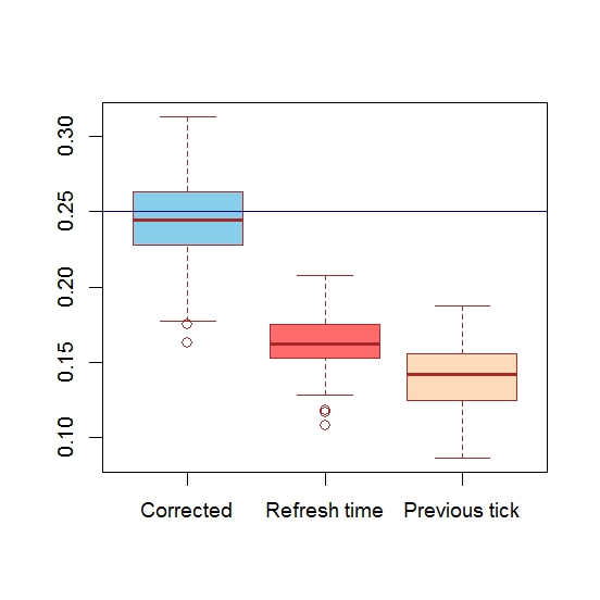
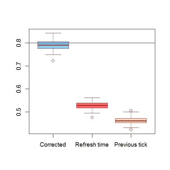
In the following simulation study, we test the performance of the method, prescribed in Theorem 1, to estimate the copula parameter. To do so, we first choose a Gaussian copula and generate 100 instances of nonsynchronous data by the method mentioned above. Initially, both $n_{1}$ and $n_{2}$ are taken to be the same. The mean, variance and Mean Square Error of the 100 estimates are reported in Table 1 and Table 2. In Figure 9, we show the boxplots for $\rho=0.8$. The boxplot on the left corresponds to the corrected estimate and those on the middle and right corresponds to uncorrected estimates obtained from refresh time sampling and previous tick sampling respectively. The horizontal line suggests the true parameter.

References

- (1)
- Aït-Sahalia et al. (2010) Aït-Sahalia, Y., Fan, J. and Xiu, D. (2010), ‘High-frequency covariance estimates with noisy and asynchronous financial data’, Journal of the American Statistical Association 105(492), 1504–1517.
- Ait-Sahalia et al. (2005) Ait-Sahalia, Y., Mykland, P. A. and Zhang, L. (2005), ‘How often to sample a continuous-time process in the presence of market microstructure noise’, The Review of Financial Studies 18(2), 351–416.
- Barndorff-Nielsen et al. (2011) Barndorff-Nielsen, O. E., Hansen, P. R., Lunde, A. and Shephard, N. (2011), ‘Multivariate realised kernels: consistent positive semi-definite estimators of the covariation of equity prices with noise and non-synchronous trading’, Journal of Econometrics 162(2), 149–169.
- Breymann et al. (2003) Breymann, W., Dias, A. and Embrechts, P. (2003), ‘Dependence structures for multivariate high-frequency data in finance’, Quantitative Finance 3(1), 1–14.
- Buccheri et al. (2020) Buccheri, G., Bormetti, G., Corsi, F. and Lillo, F. (2020), ‘A score-driven conditional correlation model for noisy and asynchronous data: An application to high-frequency covariance dynamics’, Journal of Business & Economic Statistics pp. 1–17.
- Corsi and Audrino (2012) Corsi, F. and Audrino, F. (2012), ‘Realized covariance tick-by-tick in presence of rounded time stamps and general microstructure effects’, Journal of Financial Econometrics 10(4), 591–616.
- Embrechts et al. (2002) Embrechts, P., McNeil, A. and Straumann, D. (2002), ‘Correlation and dependence in risk management: properties and pitfalls’, Risk management: value at risk and beyond 1, 176–223.
- Epps (1979) Epps, T. W. (1979), ‘Comovements in stock prices in the very short run’, Journal of the American Statistical Association 74(366a), 291–298.
- Fan et al. (2012) Fan, J., Li, Y. and Yu, K. (2012), ‘Vast volatility matrix estimation using high-frequency data for portfolio selection’, Journal of the American Statistical Association 107(497), 412–428.
- Frey and McNeil (2002) Frey, R. and McNeil, A. J. (2002), ‘Var and expected shortfall in portfolios of dependent credit risks: conceptual and practical insights’, Journal of banking & finance 26(7), 1317–1334.
- Hayashi et al. (2005) Hayashi, T., Yoshida, N. et al. (2005), ‘On covariance estimation of non-synchronously observed diffusion processes’, Bernoulli 11(2), 359–379.
- Krishnan et al. (2009) Krishnan, C., Petkova, R. and Ritchken, P. (2009), ‘Correlation risk’, Journal of Empirical Finance 16(3), 353–367.
- Malgrat (2013) Malgrat, M. (2013), Pricing of a “worst of” option using a Copula method, PhD thesis, KTH.
- Malliavin et al. (2009) Malliavin, P., Mancino, M. E. et al. (2009), ‘A fourier transform method for nonparametric estimation of multivariate volatility’, The Annals of Statistics 37(4), 1983–2010.
- Mancino and Sanfelici (2011) Mancino, M. E. and Sanfelici, S. (2011), ‘Estimating covariance via fourier method in the presence of asynchronous trading and microstructure noise’, Journal of Financial Econometrics 9(2), 367–408.
- Muthuswamy et al. (2001) Muthuswamy, J., Sarkar, S., Low, A. and Terry, E. (2001), ‘Time variation in the correlation structure of exchange rates: high-frequency analyses’, Journal of Futures Markets: Futures, Options, and Other Derivative Products 21(2), 127–144.
- Nelsen (2007) Nelsen, R. B. (2007), An introduction to copulas, Springer Science & Business Media.
- Peluso et al. (2014) Peluso, S., Corsi, F. and Mira, A. (2014), ‘A bayesian high-frequency estimator of the multivariate covariance of noisy and asynchronous returns’, Journal of Financial Econometrics 13(3), 665–697.
- Renò (2003) Renò, R. (2003), ‘A closer look at the epps effect’, International Journal of theoretical and applied finance 6(01), 87–102.
- Salmon et al. (2006) Salmon, M., Schleicher, C. et al. (2006), ‘Pricing multivariate currency options with copulas’, Copulas: From Theory to Application in Finance, Risk Books, London .
- Xu (2008) Xu, Q. (2008), Estimating and evaluating the Archimedean-copula-based models in financial risk management: a dissertation submitted in fulfillment of the requirements for the degree of Doctor of Philosophy in Financial Economics, Massey University, Auckland, New Zealand, PhD thesis, Massey University.
- Zebedee and Kasch-Haroutounian (2009) Zebedee, A. A. and Kasch-Haroutounian, M. (2009), ‘A closer look at co-movements among stock returns’, Journal of Economics and Business 61(4), 279–294.
- Zhang (2011) Zhang, L. (2011), ‘Estimating covariation: Epps effect and microstructure noise’, Journal of Econometrics 160(1), 33–47.
- Zhang and Zhu (2016) Zhang, Z. and Zhu, B. (2016), ‘Copula structured m4 processes with application to high-frequency financial data’, Journal of Econometrics 194(2), 231–241.
Appendix A Proofs
A.1. Proof of Theorem 1:
Proof.
The conditional expectation:
This is a consequence of the assumption (as illustrated in the examples in section 2.2).
Similarly,
Then we have, and
.
Therefore,
Note that the estimate is defined as
where .
Let us define the correction factor: .
Now,
and
Therefore, , where
As is sample correlation coefficient, we know that
By Slutsky’s theorem we get,
Using we then have,
Now we need to stabilize the variance.
Note that,
Define, Then,
Therefore a simple application of delta method implies that
This completes the proof. ∎
A.2. Proof of Theorem 2.
Note that .
So
is a consistent estimator for the copula . But ’s
are unobserved, where ’s are actually observed.
Let us use the notation and
for the empirical distribution function of based on the observations
respectively. Therefore to claim that the estimated copula based
on the paired data (observed) is consistent, we have to show that-
a.s.
Suppose
. Note that by Assumption , .
Then,
This implies that
The second inequality is due to Chebyshev’s inequality and the last equality is due to . The third inequality is a consequence of asynchronicity as for each , there are at most two ’s (the preceding and the next) for which and are dependent.
Hence by Borel Cantelli Lemma, . Again as we have that, .
Now we have to show that uniform convergence will hold in this case. That is, we want to show . For any given we have a finite partition of the real line such that . This can be achieved
by taking and .
Then, . Because if
then by right continuity there exists a such that ,
hence contradicting the definition of . So between and
, jumps at least . This can happen at most
finite number of times, so . By our definition of ,
we have . Hence
If
then we have,
Now using properties of copula we can clearly see that
As both and are uniformly convergent to and respectively, the result follows. ∎
A.3. Proof of Theorem 3
(a) If you fix the point then there can be two situations depending on the position of as illustrated in Figure 12.
Firstly consider case 1. We are interested in the overlapping interval. As illustrated in Figure 13, define as the first interarrival of the first stock after , as the first interarrival of the 2nd stock after and as the first interarrival of the 2nd stock after i.e. if we start observing the process only from then the first arrival time for the second stock. As the arrival processes are Poisson processes, distributions of and are same (due to memory-less property). Denote all the subsequent interarrivals as and .
Now (for case 1),
Therefore (for case 1),
Now, and .
Define
and .
So,
Note that and . Therefore,
where Thereffore,
Similarly we can derive for case 2 by interchanging the role of and . See Figure 14. Hence for case 2 we have,
Now two cases are equally likely, .
Therefore combining both the cases we have, .
(b) Now we have to calculate .
For case 1:
Define,
Then, , where
For case 2 the derivation is similar.
(c) Following similar derivation as part (b) ,
where is the mean of defined below,
A similar derivation will establish-
∎
A.4. Proof of Lemma 1
As is independent of and symmetric around , clearly
So, . ∎
A.5. Proof of Theorem 4
Due to symmetry of two configurations, it is enough to prove the theorem for one configuration. Let us consider the 4th configuration. Here , , and .
The Kendall’s tau for this nonsynchronous configuration, as defined in section 1, is:
According to our notation, and . So, and . Let us denote the region, where , by i.e. .
A.6. Proof of Theorem 5
Due to symmetry of two configurations, it is enough to prove the theorem for one configuration. We consider the case of Figure 7 (4th configuration). Here , , and .
According to our notation, and . So,
where is the true Kendall’s tau and .