© 2019 IEEE. Personal use of this material is permitted. Permission from IEEE must be obtained for all other uses, in any current or future media, including reprinting/republishing this material for advertising or promotional purposes, creating new collective works, for resale or redistribution to servers or lists, or reuse of any copyrighted component of this work in other works.

Decision Making for Autonomous Vehicles at Unsignalized
Intersection in Presence of Malicious Vehicles

Sasinee Pruekprasert Affiliation: The authors are with the National Institute of Informatics, Hitotsubashi 2-1-2, Tokyo 101-8430, Japan
{sasinee, xiaoyi, dubut, chao_huang, kishida}@nii.ac.jp Xiaoyi Zhang Affiliation: The authors are with the National Institute of Informatics, Hitotsubashi 2-1-2, Tokyo 101-8430, Japan
{sasinee, xiaoyi, dubut, chao_huang, kishida}@nii.ac.jp Jérémy Dubut Affiliation: The authors are with the National Institute of Informatics, Hitotsubashi 2-1-2, Tokyo 101-8430, Japan
{sasinee, xiaoyi, dubut, chao_huang, kishida}@nii.ac.jp Affiliation: J.D. is also affiliated with the Japanese-French Laboratory for Informatics Chao Huang Affiliation: The authors are with the National Institute of Informatics, Hitotsubashi 2-1-2, Tokyo 101-8430, Japan
{sasinee, xiaoyi, dubut, chao_huang, kishida}@nii.ac.jp Masako Kishida Thanks: The authors are supported by ERATO HASUO Metamathematics for Systems Design Project (No. JPMJER1603), JST; J. Dubut is also supported by Grant-in-aid No.˜19K20215, JSPS. Affiliation: The authors are with the National Institute of Informatics, Hitotsubashi 2-1-2, Tokyo 101-8430, Japan
{sasinee, xiaoyi, dubut, chao_huang, kishida}@nii.ac.jp

Abstract

In this paper, we investigate the decision making of autonomous vehicles in an unsignalized intersection in presence of malicious vehicles, which are vehicles that do not respect the law by not using the proper rules of the right of way. Each vehicle computes its control input as a Nash equilibrium of a game determined by the priority order based on its own belief: each of non-malicious vehicle bases its order on the law, while a malicious one considers itself as having priority. To illustrate the effectiveness of our method, we provide numerical simulations, with different scenarios given by different cases of malicious vehicles.

I Introduction

Autonomous vehicles have a promising future of making transportation time effortless and enabling the driver to partake in other activities and therefore change everyday life across the world. The greatest strength of autonomous vehicle is to avoid traffic accidents caused by human error, and thus to improve safety on roadways [1]. With the development of autonomous vehicles, the focus in research moves towards complex traffic scenarios such as intersections.

Intersections, at which multiple roads and opposing directions of traffic meet together, are designed to prevent traffic jams by easing the flow of traffic. The intersections can be divided into signalized intersections and unsignalized intersections [2]. The signalized intersections have signs and signals to regulate traffic while the unsignalized intersections do not. The unsignalized intersections are typically found where the traffic flow is low. However, they usually have higher collision frequencies than the signalized intersections due to driver’s indecision. One report of National Highway Traffic Safety Administration (NHTSA) in 2011 indicates that 40 $\%$ of car collisions in the U.S. happen at intersections and 60 $\%$ of them are related to unsignalized intersections [3]. It is expected that the autonomous vehicle can efficiently avoid intersection mishap by making appropriate decisions and orchestrating proper actions without driver’s intention.

The decision making by autonomous vehicle at unsignalized intersections is a critical problem. Several approaches have been recently proposed. One common way is to investigate the human behaviour in unsignalized intersection in order to create a naturalistic decision process [4, 5]. For example, [6] proposes a human-like decision-making algorithm based on the human drivers’ data. A cooperative approach is developed for collision avoidance at intersections based on formal control theoretic techniques [7]. However, the approach requires vehicle-to-vehicle communication and thus is not scalable to general intersection handling. The principle of reachability-based decision-making approach, which predicts the probability of future collisions using error propagation, is applicable to frontal collision avoidance at intersections [8]. However, this approach may lead to conservative results. An intention-aware decision-making model for unsignalized intersections is studied in [9], where drivers’ intentions are modelled using two-layered hidden Markov models. However, the intention estimation is deterministic.

This paper uses game theory for the decision making. Game theory is the study of decision making where the players (e.g. vehicles) make choices by maximising their own expected utility based on the possible actions of other players. Thus, game theory provides a promising framework for scenarios where interactions are involved and has been widely used in various areas such as robotics [10] and economy [11]. There are also many examples of using game theory in intelligent transport systems. A game theoretic approach for modelling the flow of vehicles in a road with lane change is proposed in [12]. A cooperative strategy in non-zero-sum games is applicable to solving conflict situations between two autonomous vehicles in a roundabout [13]. The decision making based on $k$ -level games are studied for two autonomous vehicles at unsignalised intersections [14] and roundabouts [15]. In our previous work [16], we proposed a decision making for multiple autonomous vehicles at roundabouts based on Nash equilibria.

This paper proposes two main contributions. First, we propose a game-theoretic decision making of multiple autonomous vehicles in an unsignalized intersection using Nash equilibria in a perfect information game. Instead of using the concept of “aggressiveness” value proposed in [16], we determine the decision order of the vehicles based on their priorities (e.g., based on the rules of the right of way). Second, we consider aggressive and unpredictable driving behaviours of malicious vehicles to simulate the real complex traffic environment. Before the widespread adoption of the autonomous vehicles, the human drivers need to share roads with autonomous vehicles. For this reason, we classify the drivers using different levels of maliciousness, describing vehicles breaking the law, or having irrational behaviours.

The remainder of this paper is organised as follows. First, we formulate the problem in Section II. The game-theoretic decision making approach is presented in Section III. Then, Section IV introduces the design of formalising priorities. After validating the performance of the proposed method in Section V, Section VI draws the conclusions.

II Problem formulation

II-A Vehicles at unsignalised intersection

We consider autonomous vehicles in a four-way unsignalized intersection. We assume that vehicles are driving on the left and that there are at most four vehicles at the intersection, entering from different directions. Their decision making depends on the vehicles that are going to enter or are already engaged in the intersection, but not on those that have already left the intersection. We also assume that every vehicle knows which way every other vehicle is intending to use, as every vehicle declares its intention using their turn signal.

II-B Vehicle configurations

We focus on the high-level decision making of autonomous vehicles following a precomputed path. For this reason, we do not consider the path trackers and the low-level control layer in this work. So then, we over-approximate the road occupancy of each vehicle using three circles (much as [17], see Fig. 1) and assume that the vehicles perfectly follow the given navigation paths.

Refer to caption — Fig. 1: Road occupancy by over-approximation

Much as [16], we consider the case where the navigation path of each vehicle $i$ is fixed and denoted by $\mathit{path}(i)\in\{$ “straight”,“turn right”,“turn left” $\}$ . Thus, each vehicle can only control its acceleration along the given navigation path at each time step. More specifically, at each time step $t$ , each vehicle $i$ chooses its acceleration $a_{i}(t)$ in a finite set in order to minimise their overall cost functions.

The configuration of the vehicle $i$ at time step $t$ is denoted by:

X_{i}(t)=[x_{i}(t),y_{i}(t),v_{i}(t),a_{i}(t),\text{sta}_{i}(t)]^{\top}

(1)

where $(x_{i}(t),y_{i}(t))$ is the position of the vehicle $i$ (where $(0,0)$ is the center of the intersection), $v_{i}(t)$ is its velocity, $a_{i}(t)$ is its acceleration, and $\text{sta}_{i}(t)\in\{\text{``entering'' },\text{``inside'' },\text{``leaving''}\}$ is its current status (i.e., not yet entered, already inside the intersection, or far enough from the centre of the intersection) respectively.

Then, given the control input, that is, the acceleration $a_{i}(t)$ , the configuration at time step $t+1$ is represented by:

X_{i}(t+1)=F_{i}(X_{i}(t),a_{i}(t)),

(2)

where the function $F_{i}$ is computed from the navigation path and returns the configuration of the vehicle $i$ after one time step, assuming the vehicle has constant acceleration $a_{i}(t)$ between the time steps $t$ and $t+1$ .

II-C Rules for the right of way

For this paper, we use Japanese rules for deciding priorities of vehicles [18]. Rules are slightly different in other countries, especially on the side that have more priority (e.g., left in Japan [18], right in Australia [19]). Each vehicle intending to enter an unsignalized intersection then has to give the right of way to any vehicle (in order of importance):

A)

already engaged in the intersection,
B)

on its left-hand side,
C)

significantly closer to the intersection.

A vehicle can proceed and engage in the intersection, as long as it does not cross the way of a vehicle to which it should have given the right of way. In Section IV, we describe more precisely how we implement these rules in our decision making.

II-D Levels of maliciousness

type	angelic	inter.	demonic	irrational
initial.	right of way	selfish		none
S.IV-A	S.II-C	i.e. highest priority		none
decision	Nash equilibrium			random
making
S.III
update	right of way	fitting	none
priority	+
S.IV-B	fitting

Fig. 2: Summary of the different level of maliciousness

In this paper, we consider four kinds of vehicles (see Fig. 2):

•

Angelic. Such a vehicle tries to follow the rules of Section II-C and to avoid any collision.
•

Intermediate. Such a vehicle does not follow the rules from Section II-C by initially considering that it has priority. However, it may give priority to other vehicles if the situation requires it.
•

Demonic. Such a vehicle is selfish: it does not respect the rules and believes that it always has the priority. However, it considers other vehicles’ behaviours in its decision making.
•

Irrational. Such a vehicle randomly chooses its acceleration at every time step, independently of the situation.

Our goal is to see how our ego vehicle – considered as angelic – behaves in presence of different types of vehicles, including some that do not respect the rules, at different degrees of severity.

II-E Structure of the decision making

In the following two sections, we describe more precisely our decision making for autonomous vehicles with different levels of maliciousness. Our method consists of two main components: maintaining priority orders (Section IV), and computing the control inputs (Section III). Both components depend on the computations of Nash equilibria (Section III-A), similarly to our previous paper [16].

III Control inputs and predictions, as Nash equilibria

Other than irrational vehicles, each vehicle determines its acceleration based on rational decision making. In this section, we discuss a game-theoretic approach to the problem, similarly to [16]. Using the concept of priority order that we will describe more precisely in Section IV, we formulate the decision making problem as a finite perfect-information game. The players are non-cooperative vehicles, and they try to minimise their cost.

III-A $n$ -player game with perfect information

We consider $1$ -round sequential games with perfect and complete information $G=(P,\Gamma,(H_{1},\ldots,H_{n}))$ where:

•

$P=\{1,\ldots,n\}$ is a finite set of players,
•

$\Gamma$ is a finite set of strategy profiles,
•

$H_{j}:\Gamma^{n}\rightarrow\mathbb{R}$ is the cost function for player $j$ .

In such a game, every player chooses a strategy profile from $\Gamma$ to minimise its cost function. We are particularly interested in Nash equilibria, that is, a set of strategies $\gamma_{1}$ , …, $\gamma_{n}$ for every player that is optimal in the sense that for every player $j$ , for every strategy $\gamma_{j}^{\prime}$ :

H_{j}(\gamma_{1},\ldots,\gamma_{n})\leq H_{j}(\gamma_{1},\ldots,\gamma_{j}^{\prime},\ldots,\gamma_{n})

When a total order $\prec$ on the set of players is given, it is possible to compute such a Nash equilibrium by backward induction: intuitively, the order $\prec$ gives an order with which the players choose their strategy in such a way they ensure optimality.

We invite an interested reader to take a look at usual textbooks, much as [20], for more details on game theory.

III-B Cost functions for the decision making in an intersection

III-B1 Cost at each time step

We first introduce the cost of a vehicle at each time step, which we call the step-cost. The step-cost of the vehicle $i$ is given by

S_{i}(\bm{X},\prec)=\phi_{i}^{\mathit{safe}}(\bm{X},\prec)+\phi_{i}^{\mathit{velo}}(\bm{X})

(3)

where $\bm{X}$ is a vector of configurations as in (1), i.e.,

\bm{X}=[X_{1}^{\top},\ldots,X_{n}^{\top}]^{\top}

and $\prec$ is a total order on the set of vehicles.

III-B2 Safety

For each pair of vehicles $i$ and $k$ , let $d(k,i)$ be the distance between their occupancy, given by the union of three circles (see Section II-B and Fig. 1).

With this, we define the safety feature by

\phi_{i}^{\mathit{safe}}(\bm{X},\prec)=\sum_{k\neq i}\phi_{i}^{k}(\bm{X},\prec),

where

\phi_{i}^{k}(\bm{X},\prec)=\begin{cases}0&\mbox{if }\text{sta}_{i}=\mbox{``leaving''},\\ \hbox{\multirowsetup 0}&\mbox{else if the navigation paths}\\ &\mbox{of }i\mbox{ and }k\mbox{ do not collide},\\ 0&\mbox{else if }d(k,i)\geq D,\\ C_{\mathit{d}}\cdot(D-d(k,i))^{2}&\mbox{else if }d(k,i)\leq D_{\mathit{danger}},\\ \hbox{\multirowsetup 0}&\mbox{else if }i\mbox{ is minimal for }\prec\\ &\mbox{i.e. }i\mbox{ have highest priority},\\ C_{\mathit{n}}\cdot(D-d(k,i))^{2}&\mbox{otherwise}\end{cases}

(4)

Here, $0<C_{\mathit{n}}\ll C_{\mathit{d}}$ , $0<D_{\mathit{danger}}<D$ are given constants. The intention is that, as long as there is no danger of collision, the vehicle $i$ does not care about safety, but when there is a possibility of collision, the closer the vehicle $k$ is, the more careful the vehicle $i$ is. A special case is when the vehicle $i$ has the highest priority, where $i$ cares less about safety. This case is in order to break symmetric situations where all vehicles would be too conservative.

III-B3 Velocity

Let $v_{\mathit{l}}$ be the speed limit of the road. We define the velocity feature by

\phi_{i}^{\mathit{velo}}(\bm{X})=\begin{cases}C_{\mathit{u}}\cdot(v_{\mathit{l}}-v_{i})^{2}&\mbox{if }v_{\mathit{l}}\geq v\\ C_{\mathit{o}}\cdot(v_{\mathit{l}}-v_{i})^{2}&\mbox{otherwise}\end{cases}

(5)

Here, we choose $0<C_{\mathit{u}}\ll C_{\mathit{o}}$ so that each vehicle obeys the law.

III-B4 Accumulated cost function

We construct the accumulated cost function based on the receding horizon control approach [21], which determines the control inputs of the vehicles based on the predicted future up to a horizon time step $h<\infty$ .

Given a vector of accelerations $\bm{a}=[a_{j}(s)]_{j\in N,0\leq s\leq h-1}$ , define $K_{j}(\bm{X},\prec,\bm{a})=\sum\limits_{s=0}^{h-1}\,\lambda^{s}\cdot S_{j}(\widehat{X}(\bm{a},s),\prec)$ where $\lambda$ is the discounted factor and $\widehat{X}(\bm{a},s)$ is defined by induction on $s$ :

•

$\widehat{X}(\bm{a},0)=\bm{X}$ ,
•

$\widehat{X}(\bm{a},s+1)=[F_{k}(\widehat{X}_{k}(\bm{a},s),a_{k}(s)]_{k\in N}$ .

III-C Decision game

In a very similar spirit as [16], we describe a collection of games whose players are the vehicles at the intersection. Assume that a total order $\prec$ on the set of vehicles and a vector of configurations $\bm{X}$ are given. We define the game $G_{\bm{X},\prec}$ as follows:

•

The set $P$ of players is the set of vehicles.
•

The set $\Gamma$ is a finite set of acceleration patterns, that is, a finite subset of $\mathbb{R}^{h}$ , where $h$ is the time horizon.
•

For every vehicle $j$ , $H_{j}(\bm{a})=K_{j}(X,\prec,\bm{a})$ .
•

The order is given by $\prec$ .

We can then compute a Nash equilibrium using backward induction as described in Section III-A. This produces a collection of acceleration patterns that we denote by

\bm{a}(\bm{X},\prec)=[a_{j}(s,\bm{X},\prec)]_{j\in N,0\leq s\leq h-1}.

The intention of $a_{j}(s,\bm{X},\prec)$ is to be a prediction of the acceleration of the vehicle $j$ after $s$ time steps, starting from the configuration $\bm{X}$ , considering $\prec$ as the priority order.

III-D Computing control inputs and predicted configurations

Consider a vehicle $i$ that is not irrational. At each time step $t$ , the vehicle $i$ observes the precise configuration $\bm{X}(t)$ of every car. It also maintains a priority order $\prec_{i,t}$ , a total order on the set of vehicles. We will see in Section IV how this order is initialised and updated.

From those data, the vehicle $i$ can consider the game $G_{\bm{X}(t),\prec_{i,t}}$ , and then compute a Nash equilibrium as previously. We then obtain:

•

the control input $a_{i}(t)$ of the vehicle $i$ at time step $t$ given by $a_{i}(0,\bm{X}(t),\prec_{i,t})$ ,
•

a prediction $\widehat{a}_{i,j}(t)$ by the vehicle $i$ of the acceleration of the vehicle $j$ at time step $t$ .

From these predicted accelerations, the vehicle $i$ can compute a prediction of the configuration of the vehicle $j$ at time step $t+1$ by:

\widehat{X}_{i,j}(t+1)=F_{j}(X_{j}(t),\widehat{a}_{i,j}(t))

III-E Resolving deadlocks

The previous subsection described a way of computing the control input by solving a game. This method can however lead to deadlocks, that is, situations where no vehicle takes the decision to go on, and every vehicle waits for others to take the lead. This would typically happen when there is a vehicle in each of the four ways, and that there is no clear priority order that would resolve the situation. Formally, for a vehicle $i$ that is not irrational, this case is to be considered when:

1.

the velocities of all vehicles are zero, and
2.

the accelerations of all vehicles are precisely predicted using $\prec_{i,t}$ .

In the theory of concurrent system, it is known that it is impossible to avoid such a situation using only deterministic choices, and a solution is to introduce some randomness to resolve the situation [22].

A vehicle $i$ can unlock the situation in two cases:

•

either when detecting a deadlock and considering having the highest priority, that is, $i$ being minimal for $\prec_{i,t}$ ,
•

or when $i$ already detected a deadlock at time $t-1$ .

In those cases, the vehicle $i$ set its acceleration $a_{i}(t+1)$ without following a Nash equilibrium. Concretely, in our simulations, this vehicle $i$ can set its acceleration $a_{i}(t+1)$ to $10m/s^{2}$ with probability 0.25, which will ultimately break the symmetry of a deadlock situation.

IV Formalising Priorities

Again, other than irrational vehicles, each vehicle assumes some total order. In this section, we describe how each of those vehicles $i$ initialises and updates a total order $\prec_{i,t}$ on the set of vehicles. This process depends on the type of the vehicle. This is the main difference from [16], where the order $\prec$ was deduced from the behaviours of other cars, described by their “aggressiveness” values. In this paper, the order is obtained from the rules of the right of way, and by the character angelic/demonic of the cars.

IV-A Initialising priorities

IV-A1 Angelic case

Let us assume first that the vehicle $i$ is angelic. In this case, the vehicle $i$ will try to comply to the rules of the right of way as in Section II-C. For that reason, the vehicle $i$ initialises its priority order $\prec_{i,0}$ by randomly choosing a total order that satisfies the following:

A)

If $\text{sta}_{j}=$ “inside” and if $\text{sta}_{k}\neq$ “inside”, then $j\prec_{i,0}k$ .
B)

Else, if the number of vehicles is less than 4 and $j$ is “on the left-hand side” of $k$ , $j\prec_{i,0}k$ .
C)

Else, let $d_{j}$ and $d_{k}$ be the distances of $j$ and $k$ from the centre of the intersection, respectively. If $j$ is significantly closer to the centre of the intersection than $k$ , meaning that $d_{k}-d_{j}>2$ meters, then $j\prec_{i,0}k$ .

IV-A2 Selfish cases

Now, let us assume that the vehicle $i$ is demonic or intermediate. Such a vehicle will consider itself as initially having priority, and will not care about other vehicles. So the vehicle $i$ will initialise its priority order $\prec_{i,0}$ by randomly choosing any total order on the set of vehicles such that $i$ is the lowest element $i\prec_{i,0}j$ for all $j\neq i.$

IV-B Updating the priority predictions

As explained in Section II-D, demonic vehicles do not update their priority order, while intermediate and angelic ones do. Thus, if the vehicle $i$ is demonic, we always have $\prec_{i,t+1}=\prec_{i,t}$ for any time step $t$ . If the vehicle $i$ is angelic or intermediate, it will update its priority only when necessary: when the priority from the rules of the right of way changes and when its predictions are imprecise.

IV-B1 Update according to the rules of the right of way

If the vehicle $i$ is angelic, $i$ always updates its priority order whenever the right of way changes. For example, when a vehicle leaves the intersection and when a vehicle that does not have priority enters the intersection. For this case, we update $\prec_{i,t+1}$ according to the current right of way in the same way as in Section IV-A. If the rule of the right of way does not change at the current time step $t$ , we use $\prec_{i,t+1}=\prec_{i,t}$ .

IV-B2 Update due to imprecise predictions

We consider this type of update for intermediate vehicles and angelic vehicles that do not use the update according to the rules of the right of way at the current time step $t+1$ . Suppose that $i$ is one of those vehicles. As in Section III-D, given the priority order $\prec_{i,t}$ and the observed configuration $\bm{X}(t)$ at the previous time step $t$ , the vehicle $i$ can predict the configurations $\widehat{X}_{i,j}(t+1)$ of any other vehicle $j$ . In the case where these predictions are different from the observed configurations $X_{j}(t+1)$ , the vehicle $i$ updates its priority order to fit more closely these new observations. To this end, the vehicle $i$ computes the Nash equilibrium of the decision game $G_{\bm{X}(t),\prec}$ for any total order $\prec$ , and choose $\prec^{\prime}$ as the total order such that:

•

The difference between predicted and observed accelerations is minimal:

$\prec^{\prime}\in\arg\min_{\prec^{\prime}}\sum\limits_{j\in N}\lvert a_{j}(0,\bm{X}_{j}(t),\prec^{\prime})-a_{j}(t+1)\rvert.$
•

If several $\prec^{\prime}$ satisfy the first condition, choose the one that gives the minimal acceleration $a_{i}(0,\bm{X}(t),\prec^{\prime})$ .

The intention of the second condition is the following: the reason why vehicle $i$ needs to change its priority order is because some vehicles are going against its believes (either the rules of the right of way for angelic, or selfishness for intermediate). In any case, the vehicle has to be particularly careful in the case it is dealing with a demonic or an irrational vehicle. We also define $\prec_{i,t+1}$ as follows:

•

If $a_{i}(0,\bm{X}(t),\prec^{\prime})\leq a_{i}(0,\bm{X}(t),\prec_{i,t})$ , $\prec_{i,t+1}\,=\,\prec^{\prime}$ .
•

Otherwise, $\prec_{i,t+1}\,=\,\prec^{\prime}$ with probability $0.25$ , and $\prec_{i,t+1}~=~\prec_{i,t}$ with probability $0.75$ .

Again the intention of the second case is to be careful in a situation where the vehicle would benefit by being more aggressive, while in a situation that contradicts its believes.

V Experimental results

To verify the effectiveness of our approach, we perform numerical simulations using Matlab 2018a and 2018b.

V-A Experiment scenario

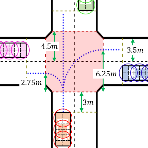
We consider four vehicles approaching an unsignalized intersection as shown in Fig. 3: each vehicle approaching from each entrance. We assume that all vehicles have rectangle shapes, and over-approximate the road occupancy of each vehicle using three circles shown in Fig. 1. We consider that two vehicles collide if their road occupancy areas intersect.

The structure of the intersection and the three navigation paths are also illustrated in Fig. 3. The navigation path type of each vehicle is randomised. The length and width of each vehicle are randomised within the range $(3.5m,5.5m)$ and $(1.5m,2.1m)$ , respectively. We consider that the navigation paths of given two vehicles do not collide only when the two vehicles approach the intersection from the opposite directions, and each vehicle either turns left or goes straight.

For each vehicle $i$ , $\text{sta}_{i}(t)$ is given as follows:

1.

$\text{sta}_{i}(t)=$ “entering” if the vehicle $i$ is approaching the intersection but none of its part has yet entered the intersection, i.e., the rectangle that represents the vehicle has not yet intersected the red area in Fig. 3.
2.

$\text{sta}_{i}(t)=$ “leaving” if more than half of the vehicle is already outside the intersection.
3.

$\text{sta}_{i}(t)=$ “inside” otherwise.

The decision making is performed every $0.1s$ . The discounted factor for the accumulated cost function is $\lambda=0.8$ . The speed limit of the road is $v_{l}=16.7m/s$ . The constant parameters are as follows: $C_{n}=20$ , $C_{d}=10^{300}$ , $D=25\,m$ , $D_{\mathit{danger}}=0.5\,m$ , $C_{u}=1$ , and $C_{o}=1000$ .

We use the following patterns of acceleration/deceleration sequences with a time horizon $h=3$ . All the accelerations in this section are in $m/s^{2}$ .

•

$[-50,-50,-50]$ for a deceleration,
•

$[0,0,0]$ for no acceleration,
•

$[10,0,0]$ for a small acceleration,
•

$[20,0,0]$ for a strong acceleration.

The accelerations of a irrational vehicle are randomly selected from the set $\{-50,0,10,20\}$ .

V-B Results and analysis

TABLE I: Simulation Results

Case	Collision rate(%)	Congestion rate(%)	Avg. Total time steps
1	0	0	56.87 (5.687s)
2	0	0.2	53.98 (5.398s)
3	0	0	59.09 (5.909s)
4	0.4	4.0	91.88 (9.988s)
1’	0	0.5	55.43 (5.543s)
2’	0	1.4	50.58 (5.058s)
3’	0	9.4	55.81 (5.581s)
4’	1.1	14.3	75.82 (7.582s)

We perform 2000 simulations for all those cases.

1

Four angelic vehicles.
2

Three angelic vehicles and one demonic vehicle.
3

Four intermediate vehicles.
4

Three intermediate vehicles and one irrational vehicle.

1000 simulations are done with initial velocity $v_{i}(0)=0$ (cases 1-4), and 1000 simulations with random initial velocity depending on the type of the vehicle (cases 1’-4’):

•

if the vehicle is demonic or irrational, we randomly choose in the interval $[0,16.7]$ m/s,
•

if the vehicle is angelic or intermediate, we randomly choose in the interval $[0,6]$ m/s.

Observe that cases 3 and 4 contain no angelic vehicles, even though we assume that the ego vehicle should be angelic. This is to see how robust the fitting method of Section IV-B is for intermediate vehicles.

As presented in Table I, we evaluate the simulations by considering the following criteria. The first column presents the collision percentage. The second column presents the percentage of the simulations that have congestions, which are situations such that: 1) there are at least two vehicles, $i$ and $j$ , such that $\text{sta}_{i}(t)=\text{sta}_{j}(t)=\mbox{``inside''}$ and 2) the navigation paths of both vehicles may collide. The third column presents the average total time that the vehicles spend running along their navigation paths.

For cases 1, 2, and 3, all vehicles successfully leave the intersection without any collisions. Some collisions are detected for the case 4, due to the unpredictable behaviour of the irrational vehicle. In the cases where the initial velocity is possibly non zero, we detect more congestions, due to the fact that vehicles have less time to make their decision before entering the intersection. However, the total time is shorter because each vehicle starts with some initial velocity.

The results also show that the vehicles may spend less time in the intersection if some of them are selfish. The case 2 is particularly interesting because it has fewer time steps than case 1. One possible explanation for this case is that the selfish vehicle makes the decision making easier: it will force itself through the intersection, so that angelic vehicles have no choice but to let it go first. After this vehicle leaves the intersection, the decision making with three vehicles is much easier.

(a) time step = 9 (b) time step = 16 (c) time step = 20

Fig. 4: A dangerous situation

In Fig. 4, we present a dangerous situation of the case 4’. The red vehicle is irrational, while the other three vehicles are intermediate. In Fig. 4(a), the red vehicle is entering the intersection, while the other three are stopped. However, in Fig. 4(b), the red vehicle suddenly stops, so the pink vehicle thinks it can enter the intersection. Finally in Fig. 4(c), the red vehicle starts again and the pink vehicle is forced to update its priority order as in Section IV-B and gives the way to the red vehicle. This scenario demonstrates that our decision making is robust enough to avoid such potential accidents.

VI Conclusion

In this paper, we propose a decision making for autonomous vehicles in a unsignalized intersection in presence of selfish and irrational vehicles. The decision is made by computing Nash equilibria of sequential games played by the vehicles. The decision orders of those games are based on the believes of which vehicles have priority: angelic vehicles define their priorities based on the rules of the right of way, while malicious ones regard themselves as having priority or do not pay any attention to priorities. We consider several scenarios where vehicles respecting the law (angelic) share the road with selfish vehicles and irrational ones, which randomly choose their accelerations. We illustrate those scenarios in our numerical simulations, demonstrating its feasibility and the robustness of our decision making in presence of malicious vehicles. As a future work, systematic experiments based on more sophisticated and practical traffic simulators will be conducted to further evaluate our model, and more detailed techniques will be adopted to eliminate the potential hazards.

References

[1] S. A. Bagloee, M. Tavana, M. Asadi, and T. Oliver, “Autonomous vehicles: challenges, opportunities, and future implications for transportation policies,” Journal of modern transportation, vol. 24, no. 4, pp. 284–303, 2016.
[2] “Unsignalized intersections,” https://safety.fhwa.dot.gov/intersection/conventional/unsignalized/.
[3] C. Hubmann, M. Becker, D. Althoff, D. Lenz, and C. Stiller, “Decision making for autonomous driving considering interaction and uncertain prediction of surrounding vehicles,” in 2017 IEEE Intelligent Vehicles Symposium (IV). IEEE, 2017, pp. 1671–1678.
[4] Y. Liu and U. Ozguner, “Human driver model and driver decision making for intersection driving,” in 2007 IEEE Intelligent Vehicles Symposium. IEEE, 2007, pp. 642–647.
[5] V. Gadepally, A. Krishnamurthy, and U. Ozguner, “A framework for estimating driver decisions near intersections,” IEEE Transactions on Intelligent Transportation Systems, vol. 15, no. 2, pp. 637–646, 2014.
[6] P. De Beaucorps, T. Streubel, A. Verroust-Blondet, F. Nashashibi, B. Bradai, and P. Resende, “Decision-making for automated vehicles at intersections adapting human-like behavior,” in 2017 IEEE Intelligent Vehicles Symposium (IV). IEEE, 2017, pp. 212–217.
[7] M. R. Hafner, D. Cunningham, L. Caminiti, and D. Del Vecchio, “Cooperative collision avoidance at intersections: Algorithms and experiments,” IEEE Transactions on Intelligent Transportation Systems, vol. 14, no. 3, pp. 1162–1175, 2013.
[8] G. R. de Campos, A. H. Runarsson, F. Granum, P. Falcone, and K. Alenljung, “Collision avoidance at intersections: A probabilistic threat-assessment and decision-making system for safety interventions,” in 17th International IEEE Conference on Intelligent Transportation Systems (ITSC). IEEE, 2014, pp. 649–654.
[9] W. Song, G. Xiong, and H. Chen, “Intention-aware autonomous driving decision-making in an uncontrolled intersection,” Mathematical Problems in Engineering, 2016.
[10] Y. Meng, “Multi-robot searching using game-theory based approach,” International Journal of Advanced Robotic Systems, vol. 5, no. 4, p. 44, 2008.
[11] G. M. Hodgson and K. Huang, “Evolutionary game theory and evolutionary economics: are they different species?” Journal of evolutionary economics, vol. 22, no. 2, pp. 345–366, 2012.
[12] A. Talebpour, H. S. Mahmassani, and S. H. Hamdar, “Modeling lane-changing behavior in a connected environment: A game theory approach,” Transportation Research Procedia, vol. 7, pp. 420–440, 2015.
[13] L. Banjanovic-Mehmedovic, E. Halilovic, I. Bosankic, M. Kantardzic, and S. Kasapovic, “Autonomous vehicle-to-vehicle (v2v) decision making in roundabout using game theory,” Int. J. Adv. Comput. Sci. Appl, vol. 7, pp. 292–298, 2016.
[14] N. Li, I. Kolmanovsky, A. Girard, and Y. Yildiz, “Game theoretic modeling of vehicle interactions at unsignalized intersections and application to autonomous vehicle control,” in Proceedings of the 2018 Annual American Control Conference (ACC), 2018.
[15] R. Tian, S. Li, N. Li, I. Kolmanovsky, A. Girard, and Y. Yildiz, “Adaptive game-theoretic decision making for autonomous vehicle control at roundabouts,” in Proceedings of the 2018 IEEE Conference on Decision and Control (CDC), 2018.
[16] S. Pruekprasert, J. Dubut, X. Zhang, C. Huang, and M. Kishida, “A game theoretic approach to decision making for multiple vehicles at roundabout,” arxiv:1904.06224, 2019.
[17] M. Cao, R. Wang, J. Wang, and N. Chen, “An integrated MPC approach for FWIA autonomous ground vehicles with emergency collision avoidance,” in Proceedings of the 21st International Conference on Intelligent Transportation Systems (ITSC), 2018.
[18] J. N. P. Agency, “To foreign nationals who drive vehicles in japan (english language version),” https://www.npa.go.jp/policies/application/license_renewal/pdf/english.pdf, 2011.
[19] N. T. Government, “Road rules in NT,” https://nt.gov.au/driving/safety/road-rules-in-nt, 2015.
[20] M. J. Osborne, An introduction to game theory. New York, NY [u.a.]: Oxford Univ. Press, 2004.
[21] W. H Kwon and S. Han, Receding Horizon Control: Model Predictive Control for State Models. Springer, 2005.
[22] D. J. Lehmann and M. O. Rabin, “On the advantages of free choice: A symmetric and fully distributed solution to the dining philosophers problem,” in Conference Record of the Eighth Annual ACM Symposium on Principles of Programming Languages (POPL’81), 1981.

Decision Making for Autonomous Vehicles at Unsignalized Intersection in Presence of Malicious Vehicles