跳到论文正文
W Papers独立论文阅读器 arXiv:1904.10077 论文正文 计算阅读时间 · 0%
引用这篇论文根据当前论文元数据生成,正式投稿前建议核对。


License: arXiv.org perpetual non-exclusive license
arXiv:1904.10077v1 [cs.NI] 22 Apr 2019

Benefits of Coding on Age of Information in Broadcast Networks

Xingran Chen    Shirin Saeedi Bidokhti Affiliation: Department of Electrical and Systems Engineering Affiliation: University of Pennsylvania Affiliation: {xingranc, saeedi}@seas.upenn.edu
Index Terms: 
Age of Information, Network Coding, Randomized Policy, Max-Weight Policy, Feedback, Broadcast Packet Erasure Channels

Abstract

Age of Information (AoI) is studied in two-user broadcast networks with feedback, and lower and upper bounds are derived on the expected weighted sum AoI of the users. In particular, a class of simple coding actions is considered and within this class, randomized and deterministic policies are devised. Explicit conditions are found for symmetric dependent channels under which coded randomized policies strictly outperform the corresponding uncoded policies. Similar behavior is numerically shown for deterministic policies.

I Introduction

Sending status updates in a timely manner has significant importance in the Internet of Things (IoT) applications. In practice, it is not always effective to update the information as fast as possible for it may cause further delay in the network queues. To measure the timeliness of information at a remote system, the concept of Age of Information (AoI) was introduced in [1, 2, 3]. AoI measures, at the receiving side, how much time has passed since the generation time of the latest received packet. In [3], a single source and server setup were considered under First-Come First-Serve (FCFS) queue management and it was shown that there is an optimal update rate that minimizes time-average AoI. Further extensions to networks of multiple sources and servers with and without packet management were studied in [4, 5, 6, 7, 8]. More recently, AoI has been studied as a performance metric in various contexts such as source and channel coding [9, 10, 11], caching [12, 13, 14], energy harvesting [15, 16, 17], sampling [18, 19, 20] and scheduling [21, 22, 23, 24, 25, 26, 27, 28, 29].

In coding theory, previous work has mainly studied point to point channels. For example, [30, 31, 32] consider erasure channels, propose coding schemes, and analyze the resulting average or peak AoI in various setups. More recently, [33] proves that when the source alphabet and channel input alphabet have the same size, a Last-Come First-Serve (LCFS) with no buffer policy is optimal. Considering erasure channels with FCFS M/G/1 queues, [34] finds an optimal block length for channel coding to minimize the average age and average peak age of information.

AoI has also been investigated in network management and scheduling. In particular, [21] proposes scheduling policies to optimize the overall age in a wireless network. Maintaining equally up-to-date and synchronized information from multiple sources is studied in [22]. In [26], scheduling algorithms are designed to minimize AoI in wireless broadcast channels. [25] devises scheduling policies to minimize average AoI under throughput constraints in wireless multi-access networks. The minimum age of time-varying wireless channels with interference constraints is obtained in [27, 28, 29] with and without channel state information.

In this work, we aim to shed light on the interplay between AoI and (channel/network) coding in the context of broadcast packet erasure channels (BPECs) with feedback. BPECs and their variants have been investigated in previous work such as [35, 36, 37, 38, 39] and rate-optimal coding algorithms are designed using (network) coding ideas. The key idea is due to [35] where it is shown that the entire capacity region of two-user BPECs with feedback can be attained by XOR-ing overheard packets. More precisely, suppose a packet pp, intended for user 11, is broadcasted and only received at user 22. Scheduling algorithms re-transmit this packet because it is not received at its intended receiver. However, one may be able to exploit coding opportunities by tracking such packets (and this is possible through the available feedback). For example, in a similar manner, a packet qq, intended for user 22, may get transmitted and received only at receiver 11. Now instead of re-transmitting pp and qq in two uses of the network, one can transmit the XOR packet p⊕qp\oplus q which is simultaneously useful for both users.

As opposed to the aforementioned literature, in this work, we seek efficiency in terms of age as opposed to rate. The underlying challenge is as follows. On the one hand, the highest rate of communication in BPECs can be attained when coding is employed across packets of different users [35]. A higher rate effectively corresponds to a smaller delay (both in the sense that the queues get emptied faster and in the sense that fewer uses of the network are needed in total to transmit a fixed number of information bits). On the other hand, to achieve high rates with coding, we have to incur delay by waiting for the arrival of other packets for the purpose of coding as well as prioritizing their transmission. So it is not clear apriori when coding is beneficial. We will devise scheduling policies that schedule different coding actions, as opposed to traditional schemes that schedule different users, and show the benefit of coding in terms of average age over uncoded schemes such as those proposed in [26].

Motivated by the capacity achieving coding scheme of [35], in this work we restrict attention to a class of coding algorithms consisting of three actions: uncoded transmission for user 11, uncoded transmission for user 22, and coded (XOR-ed) transmission for both users. We consider a discrete time model as in [26] and study the expected weighted sum of AoI (EWSAoI) at the users. The first contribution of the paper is a general lower bound on the achievable EWSAoI. As opposed to previous lower bounds (e.g. [26]) that hold only in the class of traditional scheduling algorithms, the new lower bound is valid for any coding scheme. The second contribution of the paper is the devise and analysis of EWSAoI or an upper bound on it for (i) stationary randomized policies and (ii) deterministic Max-Weight (MW) policies. In the class of randomized policies, for symmetric channels, we find conditions under which coded policies perform strictly better than their corresponding uncoded policies. For MW policies, we numerically compare the performance of coded and uncoded MW policies and show gains of coding.

The remainder of this paper is organized as follows. The problem setup and notation are introduced in Section II. Section III presents a general lower bound on EWSAoI. In Section IV, we devise a randomized policy based on three coding actions and find a closed-form expression for the resulting EWSAoI. We further study the special case of symmetric BPECs and find conditions under which coded randomized policies strictly outperform uncoded randomized policies in terms of age. In Section V, we propose a Max-Weight policy and derive an upper bound on the resulting EWSAoI. Simulation results and the comparison of uncoded vs. coded schemes are presented in Section VI.

II System Model

We consider a model where time is slotted. At the beginning of every time slot, new packets are generated for the users and they replace any undelivered packets from previous time slots. Our model is similar to [25, 26], where users are scheduled with the goal of minimizing age.

Transmission occurs on a noisy network which we model by a broadcast packet erasure channel with two users. In each time slot kk, the input X⁡(k)X(k) to the channel is a packet. The packet is successfully delivered to user ii with probability 1−ϵi1-\epsilon_{i}, 0≤ϵi<10\leq\epsilon_{i}<1, and lost with probability ϵi\epsilon_{i}. Let Zi​(k)Z_{i}(k) be a random variable modeling erasure at user i∈{1,2}i\in\{1,2\} in time slot k∈{1,2,…}k\in\{1,2,\ldots\}. We assume that the channel is memoryless and hence {Zi​(k)}k=1∞\{Z_{i}(k)\}_{k=1}^{\infty} is an iid Bernoulli process with probability 1−ϵi1-\epsilon_{i}. The output of the channel at user ii in slot kk is:

Yi​(k)={X⁡(k)if ​Zi​(k)=1Δotherwise\displaystyle Y_{i}(k)=\left\{\begin{array}[]{cc}X(k)&\text{if }Z_{i}(k)=1\\ \Delta&\text{otherwise}\end{array}\right.

where Δ\Delta is a symbol denoting erasure. Note that the pairs {(Z1​(k),Z2​(k))}k\{(Z_{1}(k),Z_{2}(k))\}_{k} are independent across time (over k=1,2,…k=1,2,\ldots) but potentially correlated across (Z1,Z2)(Z_{1},Z_{2}). In addition, the feedback is available at the encoder after each transmission. Define ϵ1,ϵ2,ϵ12\epsilon_{1},\epsilon_{2},\epsilon_{12} as

ϵ1:=\displaystyle\epsilon_{1}:= Pr⁡(Z1=0)\displaystyle\Pr(Z_{1}=0)
ϵ2:=\displaystyle\epsilon_{2}:= Pr⁡(Z2=0)\displaystyle\Pr(Z_{2}=0)
ϵ12:=\displaystyle\epsilon_{12}:= Pr⁡(Z1=0,Z2=0),\displaystyle\Pr(Z_{1}=0,Z_{2}=0),

and hence we have

Pr⁡(Z1=1,Z2=0)=\displaystyle\Pr(Z_{1}=1,Z_{2}=0)= ϵ2−ϵ12\displaystyle\epsilon_{2}-\epsilon_{12}
Pr⁡(Z1=0,Z2=1)=\displaystyle\Pr(Z_{1}=0,Z_{2}=1)= ϵ1−ϵ12.\displaystyle\epsilon_{1}-\epsilon_{12}.

The statistics of (Z1,Z2)(Z_{1},Z_{2}) that describes the channel is assumed fixed and given and can be characterized by (ϵ1,ϵ2,ϵ12)(\epsilon_{1},\epsilon_{2},\epsilon_{12}).

We consider a simple class of coding algorithms that consists of three actions, including a network coding action. The encoder is modeled by a network of virtual queues. Let Q1(i)Q_{1}^{(i)} denote the queue of incoming packets for user ii and Q2(i)Q_{2}^{(i)} denote the queue of packets that are intended for user ii but are received only by the other user. The encoder can track such packets using the available feedback. For i={1,2}i=\{1,2\}, we use the notation \i\backslash i as short for {1,2}\i\{1,2\}\backslash i. The packets in Q2(i)Q_{2}^{(i)} are not received at their intended receivers, but are received at the other receiver and act as side information for it – this can be exploited in the code design at the encoder. In particular, the encoder can XOR packets in Q2(1)Q_{2}^{(1)} with Q2(2)Q_{2}^{(2)} and form more efficient coded packets for transmission.

In each time slot kk, the encoder decides between the following three actions, denoted by A⁡(k)∈{1,2,3}A(k)\in\{1,2,3\} and defined below:

  • •

    A⁡(k)=1A(k)\!=\!1: a packet is transmitted from Q1(1)Q_{1}^{(1)};

  • •

    A⁡(k)=2A(k)\!=\!2: a packet is transmitted from Q1(2)Q_{1}^{(2)};

  • •

    A⁡(k)=3A(k)\!=\!3: a coded packet is transmitted from Q2(1)Q_{2}^{(1)}, Q2(2)Q_{2}^{(2)}.

Refer to caption
Fig. 1: the virtual network of queues at the encoder
Definition 1 (Age of Information [1]).

Consider a source-destination pair. Let {tk}k\{t_{k}\}_{k} be the times at which packets are generated and {tk′}k\{t_{k}^{\prime}\}_{k} be the times at which packets are received at the destination. At any time ξ\xi, denote N⁡(ξ)=max⁡{k|tk′≤ξ}N(\xi)=\max\{k|t_{k}^{\prime}\leq\xi\}, and u⁡(ξ)=tN⁡(ξ)u(\xi)=t_{N(\xi)}. The Age of Information (AoI) at the destination is Δ⁡(t)=t−u⁡(t)\Delta(t)=t-u(t).

Using Definition 1, let hih_{i} be the positive real number that represents the age at user ii. The age hih_{i} increases linearly in time when there is no delivery of packets to user ii and drops with every delivery to a value that represents how old the received packet is.

Lemma 1.

To attain the optimal age in the above class of 3−3-action coding algorithms, we can assume, without loss of generality, that all queues are of buffer size 11.

Proof.

The proof is presented in Appendix A. ∎

To capture the evolution of hih_{i} in the class of 3−3-action algorithms described, we proceed as follows. First, define wi​(k)w_{i}(k) as the (current) age of information at Q2(i)Q_{2}^{(i)} in slot kk. If the packet in Q2(i)Q_{2}^{(i)} is successfully delivered at user ii by time kk, then it is removed from Q2(i)Q_{2}^{(i)} and wi​(k)w_{i}(k) is defined to be zero; if a packet in Q2(i)Q^{(i)}_{2} is replaced by a new packet pp in slot kk, then wi​(t)w_{i}(t) is the age of the new packet when t>kt>k. More precisely, suppose packet pp is generated at time tpt_{p}. At time tt, while pp is in the queue Q2(i)Q_{2}^{(i)}, the age w⁡(t)w(t) is t−tpt-t_{p}. Finally, once a packet is delivered successfully at user ii from Q1(i)Q_{1}^{(i)}, then the existing packet in Q2(i)Q_{2}^{(i)} (which is necessarily older) becomes obsolete and hence we remove it from Q2(i)Q_{2}^{(i)} and define wi​(k+1)w_{i}(k+1) to be 00. Thus, the recursion of wi​(k)w_{i}(k) is

wi(k+1)={0​if​A​(k)∈{i,3},Zi​(k)=11​if​A​(k)=i,(Zi​(k),Z\i​(k))=(0,1)(wi(k)+1)⋅1{wi(k)>0}otherwise.\displaystyle\footnotesize w_{i}(k+1)=\left\{\begin{aligned} &0\,\,\text{if}\,A(k)\in\{i,3\},\,Z_{i}(k)=1\\ &1\,\,\text{if}\,A(k)=i,\,(Z_{i}(k),Z_{\backslash{i}}(k))=(0,1)\\ &(w_{i}(k)+1)\cdot 1_{\{w_{i}(k)>0\}}\,\,\text{otherwise}\end{aligned}\right.. (1)

Based on wi​(k)w_{i}(k), the age function hi​(k)h_{i}(k) evolves as follows:

hi(k+1)={1​if​A​(k)=i,Zi​(k)=1wi​(k)+1​if​A​(k)=3,Zi​(k)=1hi​(k)+1​otherwise.\displaystyle\footnotesize h_{i}(k+1)=\left\{\begin{aligned} &1\hskip 8.50012pt\text{if}\,\,A(k)=i,\,Z_{i}(k)=1\\ &w_{i}(k)+1\hskip 8.50012pt\text{if}\,\,A(k)=3,\,Z_{i}(k)=1\\ &h_{i}(k)+1\hskip 8.50012pt\text{otherwise}\end{aligned}\right.. (2)
Remark 1.

Using the mathematical recursions in (1) and (2), we conclude that wi​(k)≤hi​(k)−1w_{i}(k)\leq h_{i}(k)-1.

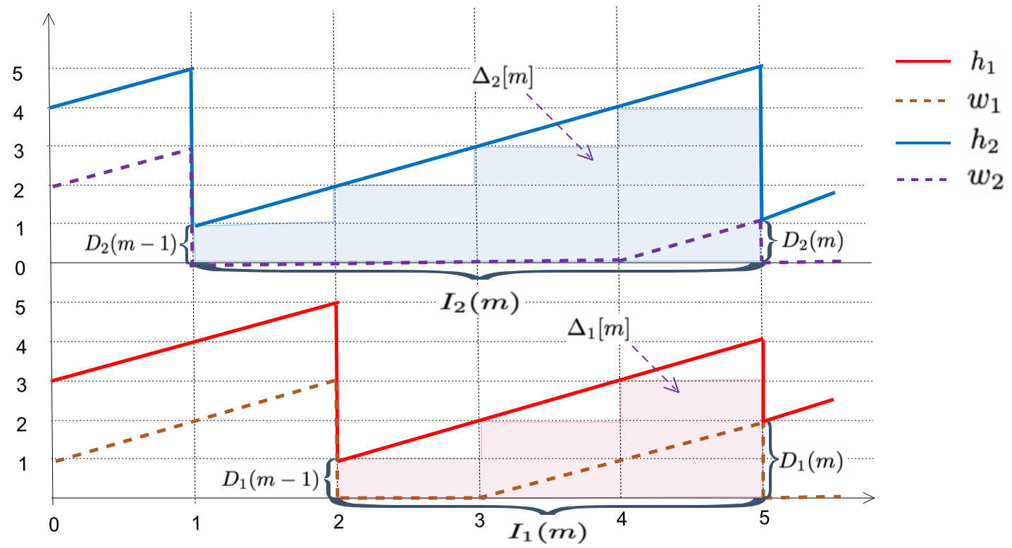
Refer to caption
Fig. 2: a sample path of the channel state (h1,h2,w1,w2)(h_{1},h_{2},w_{1},w_{2}) which initial state (h1,h2,w1,w2)=(3,4,1,2)(h_{1},h_{2},w_{1},w_{2})=(3,4,1,2)

II-A A Sample Path

A sample path for the evolution of w1,h1w_{1},h_{1} and w2,h2w_{2},h_{2} is shown in Fig. 2. The initial state is (h1,h2,w1,w2)=(3,4,1,2)(h_{1},h_{2},w_{1},w_{2})=(3,4,1,2), and the actions and the channels are as follows:

kk 1 2 3 4 5
A⁡(k)A(k) 2 1 1 2 3
(Z1​(k),Z2​(k))(Z_{1}(k),Z_{2}(k)) (1,1) (1,0) (0,1) (1,0) (1,1)

Now consider a general sample path associated with a transmission policy and a finite time-horizon TT. For this sample path, let Ni​(T)N_{i}(T) be the total number of packets delivered to user ii up to and including time slot TT, and Ii​(m)I_{i}(m) be the number of time slots between the (m−1)(m-1)th and mmth deliveries to user ii, i.e., the inter delivery times of user ii. Denote the age of user ii after delivery of the mmth packet by Di​(m)D_{i}(m) and let LiL_{i} be the number of remaining time slots after the last packet delivery to the same user. With this notation, the time-horizon can be written as T=∑m=1Ni​(T)Ii​(m)+LiT=\sum_{m=1}^{N_{i}(T)}I_{i}(m)+L_{i} with i∈{1,2}i\in\left\{1,2\right\}.

Next, consider the sum of the instantaneous ages in the interval corresponding to Ii​(m)I_{i}(m), m≥2m\geq 2, denoted by Δi​[m]\Delta_{i}[m]. As shown in Figure 2, Δi​[m]\Delta_{i}[m] is equal to the area underneath the age curve in the corresponding interval minus Ii​(m)I_{i}(m) small triangle areas; i.e.,

Δi​[m]=∑k​ in between delivery of m−1​t​h and mth packetshi​[k]\displaystyle\Delta_{i}[m]=\sum_{k\text{ in between delivery of ${m-1}^{\text{}th}$ and $m^{\text{th}}$ packets}}h_{i}[k] (3)
=\displaystyle= (Di​(m−1)+Ii​(m))22−(Di​(m−1))22−Ii​(m)2\displaystyle\frac{(D_{i}(m-1)+I_{i}(m))^{2}}{2}-\frac{(D_{i}(m-1))^{2}}{2}-\frac{I_{i}(m)}{2} (4)
=\displaystyle= Ii2​(m)2+Di​(m−1)​Ii​(m)−Ii​(m)2.\displaystyle\frac{I_{i}^{2}(m)}{2}+D_{i}(m-1)I_{i}(m)-\frac{I_{i}(m)}{2}. (5)

II-B The Expected Weighted Sum AoI

Both wi​(k)w_{i}(k) and hi​(k)h_{i}(k) and their evolution depend on the policy that we choose and, hence, we sometimes write them as wiπ​(k)w_{i}^{\pi}(k) and hiπ​(k)h_{i}^{\pi}(k). Moreover, we denote the vector (h1​(1),h2​(1),w1​(1),w2​(1))(h_{1}(1),h_{2}(1),w_{1}(1),w_{2}(1)) by s→​(1)\vec{s}(1).

We aim to find policies π\pi that minimize the following EWSAoI at the users:

𝔼⁡[12​T​∑k=1T∑i=12αi​hiπ​(k)|s→​(1)]\displaystyle\mathbb{E}\left[\frac{1}{2T}\sum_{k=1}^{T}\sum_{i=1}^{2}\alpha_{i}h^{\pi}_{i}(k)\Big|\vec{s}(1)\right] (6)

where α1\alpha_{1} and α2\alpha_{2} are weights associated to users 11 and 22, respectively. We assume αi≥0\alpha_{i}\geq 0 and α1+α2=1\alpha_{1}+\alpha_{2}=1. For notational simplicity, we omit s→​(1)\vec{s}(1) hereafter, and hence the minimum age is given by the following optimization problem.

minπ∈Π⁡𝔼⁡[JTπ],whereJTπ=12​T​∑k=1T∑i=12αi​hiπ​(k).\displaystyle\min_{\pi\in\Pi}\mathbb{E}[J_{T}^{\pi}],\quad\text{where}\quad J_{T}^{\pi}=\frac{1}{2T}\sum_{k=1}^{T}\sum_{i=1}^{2}\alpha_{i}h_{i}^{\pi}(k). (7)

Since we aim to minimize the EWSAoI in the long run, we define

Jπ=limT→∞JTπ.\displaystyle J^{\pi}=\lim_{T\rightarrow\infty}J_{T}^{\pi}.

III A Lower Bound

We prove a lower bound on EWSAoI as stated below.

Theorem 1.

For any communication policy π\pi, we have:

𝔼⁡[Jπ]≥14​((∑i=12αi​(2−ϵ12−ϵ\i))2(1−ϵ12)​(2−ϵ1−ϵ2)+1).\displaystyle\mathbb{E}[J^{\pi}]\geq\frac{1}{4}\left(\frac{(\sum_{i=1}^{2}\sqrt{\alpha_{i}(2-\epsilon_{12}-\epsilon_{\backslash{i}})})^{2}}{(1-\epsilon_{12})(2-\epsilon_{1}-\epsilon_{2})}+1\right). (8)
Remark 2.

The lower bound of Theorem 1 holds in general and is not restricted to the class of 3−3-action coded algorithms that we introduced in Section II.

Proof.

Consider a sample path associated with a transmission policy and a finite time-horizon TT (see Section II-A). The EWSAoI as defined in (6) can be re-written in terms of Δi​(m)\Delta_{i}(m)’s:

JTπ=\displaystyle J_{T}^{\pi}= 12​T​∑k=1T∑i=12αi​hi​(k)\displaystyle\frac{1}{2T}\sum_{k=1}^{T}\sum_{i=1}^{2}\alpha_{i}h_{i}(k)
=\displaystyle= 12​∑i=12αiT​(∑m=1Ni​(T)Δi​(m)+12​Li2+Di​(Ni​(T))​Li−12​Li).\displaystyle\frac{1}{2}\!\sum_{i=1}^{2}\!\frac{\alpha_{i}}{T}\!\!\left(\!\sum_{m=1}^{N_{i}(T)}\!\!\!\!\Delta_{i}(m)\!+\!\frac{1}{2}L_{i}^{2}\!+\!D_{i}(\hskip-1.42271ptN_{i}(\hskip-1.42271ptT\hskip-1.42271pt)\hskip-1.42271pt)L_{i}\!-\!\frac{1}{2}L_{i}\!\!\right)\!\!. (9)

Since Di​(m)≥1D_{i}(m)\geq 1 for all 1≤m≤Ni​(T)1\leq m\leq N_{i}(T), we can lower bound (5) and hence (III) by substituting Di​(m)=1D_{i}(m)=1. Using similar steps as [26, Eqns. (9) - (14)], we find

JTπ≥14​∑i=12αi​TNi​(T)+14.\displaystyle J^{\pi}_{T}\geq\frac{1}{4}\sum_{i=1}^{2}\alpha_{i}\frac{T}{N_{i}(T)}+\frac{1}{4}. (10)

We remark that so far, the lower bound on JTπJ_{T}^{\pi} is the same as [26, Eqn. (7)]. We now depart from [26] by allowing for the general class of coding and scheduling schemes. Recall that Ni​(T)N_{i}(T) is the total number of packets received by user ii, i=1,2i=1,2. In the limit of T→∞T\to\infty, Ni​(T)T\frac{N_{i}(T)}{T} is the throughput of user ii. We further know the capacity of two-user broadcast packet erasure channels from [35]. In particular, any non-negative rate pair (R1,R2)(R_{1},R_{2}) is achievable if and only if it satisfies the following conditions.

R11−ϵ1+R21−ϵ12≤1\displaystyle\frac{R_{1}}{1-\epsilon_{1}}+\frac{R_{2}}{1-\epsilon_{12}}\leq 1 (11)
R11−ϵ12+R21−ϵ2≤1.\displaystyle\frac{R_{1}}{1-\epsilon_{12}}+\frac{R_{2}}{1-\epsilon_{2}}\leq 1. (12)

Hence, from (11) and (12), we have

limT→∞N1​(T)T1−ϵ1+N2​(T)T1−ϵ12≤1\displaystyle\lim_{T\rightarrow\infty}\frac{\frac{N_{1}(T)}{T}}{1-\epsilon_{1}}+\frac{\frac{N_{2}(T)}{T}}{1-\epsilon_{12}}\leq 1 (13)
limT→∞N1​(T)T1−ϵ12+N2​(T)T1−ϵ2≤1.\displaystyle\lim_{T\rightarrow\infty}\frac{\frac{N_{1}(T)}{T}}{1-\epsilon_{12}}+\frac{\frac{N_{2}(T)}{T}}{1-\epsilon_{2}}\leq 1. (14)

For notational simplicity, denote x=limT→∞N1​(T)Tx=\lim_{T\rightarrow\infty}\frac{N_{1}(T)}{T} and y=limT→∞N2​(T)Ty=\lim_{T\rightarrow\infty}\frac{N_{2}(T)}{T}. Substituting xx and yy into (13) and (14), we obtain

x1−ϵ1+y1−ϵ12≤1\displaystyle\frac{x}{1-\epsilon_{1}}+\frac{y}{1-\epsilon_{12}}\leq 1
x1−ϵ12+y1−ϵ2≤1.\displaystyle\frac{x}{1-\epsilon_{12}}+\frac{y}{1-\epsilon_{2}}\leq 1.

Re-arranging terms, we obtain

(1−ϵ12)​x+(1−ϵ1)​y≤(1−ϵ12)​(1−ϵ1)\displaystyle(1-\epsilon_{12})x+(1-\epsilon_{1})y\leq(1-\epsilon_{12})(1-\epsilon_{1})
(1−ϵ2)​x+(1−ϵ12)​y≤(1−ϵ12)​(1−ϵ2)\displaystyle(1-\epsilon_{2})x+(1-\epsilon_{12})y\leq(1-\epsilon_{12})(1-\epsilon_{2})

and summing the above two inequalities, we get

k1​x+k2​y≤k3\displaystyle k_{1}x+k_{2}y\leq k_{3} (15)

where

k1=\displaystyle k_{1}= 2−ϵ2−ϵ12\displaystyle 2-\epsilon_{2}-\epsilon_{12}
k2=\displaystyle k_{2}= 2−ϵ1−ϵ12\displaystyle 2-\epsilon_{1}-\epsilon_{12}
k3=\displaystyle k_{3}= (1−ϵ12)​(2−ϵ1−ϵ2).\displaystyle(1-\epsilon_{12})(2-\epsilon_{1}-\epsilon_{2}).

We can now use (15) along with the Cauchy-Schwarz inequality and write

(α1x+α2y)​k3\displaystyle\Big(\frac{\alpha_{1}}{x}+\frac{\alpha_{2}}{y}\Big)k_{3} ≥(α1x+α2y)​(k1​x+k2​y)\displaystyle\geq\Big(\frac{\alpha_{1}}{x}+\frac{\alpha_{2}}{y}\Big)(k_{1}x+k_{2}y)
≥(α1​k1+α2​k2)2.\displaystyle\geq\left(\sqrt{\alpha_{1}k_{1}}+\sqrt{\alpha_{2}k_{2}}\right)^{2}.

Re-arranging terms and replacing for k1,k2,k3k_{1},k_{2},k_{3}, we find

(α1x+α2y)≥(∑i=12αi​(2−ϵ\i−ϵ12))2(1−ϵ12)​(2−ϵ1−ϵ2)\displaystyle\Big(\frac{\alpha_{1}}{x}+\frac{\alpha_{2}}{y}\Big)\geq\frac{(\sum_{i=1}^{2}\sqrt{\alpha_{i}(2-\epsilon_{\backslash{i}}-\epsilon_{12})})^{2}}{(1-\epsilon_{12})(2-\epsilon_{1}-\epsilon_{2})}

and hence, from (10), we obtain

Jπ≥\displaystyle J^{\pi}\geq limT→∞14​∑i=12αi​TNi​(T)+14\displaystyle\lim_{T\rightarrow\infty}\frac{1}{4}\sum_{i=1}^{2}\alpha_{i}\frac{T}{N_{i}(T)}+\frac{1}{4}
≥\displaystyle\geq 14​((∑i=12αi​(2−ϵ12−ϵ\i))2(1−ϵ12)​(2−ϵ1−ϵ2)+1).\displaystyle\frac{1}{4}\Big(\frac{(\sum_{i=1}^{2}\sqrt{\alpha_{i}(2-\epsilon_{12}-\epsilon_{\backslash{i}})})^{2}}{(1-\epsilon_{12})(2-\epsilon_{1}-\epsilon_{2})}+1\Big).

∎

IV Coded Randomized Policies

Consider a stationary randomized policy where each action is chosen with a fixed probability in each time slot, independent of the system’s status. Denote by μi\mu_{i} the probability of action A⁡(k)=iA(k)=i, i∈{1,2,3}i\in\{1,2,3\}, k∈{1,…}k\in\{1,\ldots\}, where μ1+μ2+μ3=1\mu_{1}+\mu_{2}+\mu_{3}=1. Denote the EWSAoI for randomized policies (in the long run) as 𝔼⁡[JR]\mathbb{E}[J^{R}].

IV-A Age Analysis

We will first find the exact EWSAoI of the coded randomized policy. We start with Δi​(m)\Delta_{i}(m) derived in (5). Consider i=1i=1. The expectation of Δ1​(m)\Delta_{1}(m) is

𝔼⁡[Δ1​(m)|s→​(1)]\displaystyle\mathbb{E}[\Delta_{1}(m)|\vec{s}(1)]\! (16)
=\displaystyle= 𝔼⁡[I12​(m)2+D1​(m−1)​I1​(m)−I1​(m)2|s→​(1)]\displaystyle\!\mathbb{E}\left[\frac{I_{1}^{2}(m)}{2}+D_{1}(m-1)I_{1}(m)-\frac{I_{1}(m)}{2}\Big|\vec{s}(1)\right]\! (17)
=\displaystyle= 𝔼⁡[I12]2+𝔼⁡[D1]​𝔼​[I1]−𝔼⁡[I1]2.\displaystyle\frac{\mathbb{E}\left[{I_{1}^{2}}\right]}{2}+\mathbb{E}[D_{1}]\mathbb{E}[I_{1}]-\frac{\mathbb{E}[I_{1}]}{2}. (18)

Equality (18) holds because of the following observations: (i) the processes {I1​(m)}m\{I_{1}(m)\}_{m} and {D1​(m)}m\{D_{1}(m)\}_{m} are each iid and not dependent on s→​(1)\vec{s}(1) (so we use I1I_{1} and D1D_{1} to denote the underlying random variables, respectively), and (ii) I1​(m)I_{1}(m) and D1​(m−1)D_{1}(m-1) are independent (while I1​(m)I_{1}(m) and D1​(m)D_{1}(m) may be dependent). Thus, the EWSAoI of user 11 is

limT→∞1T​∑k=1T𝔼⁡[h1​(k)|s→​(1)]\displaystyle\lim_{T\to\infty}\frac{1}{T}\sum_{k=1}^{T}\mathbb{E}[h_{1}(k)|\vec{s}(1)] (19)
=\displaystyle= limT→∞1T​∑m=1N1​(T)𝔼⁡[Δ1​(m)|s→​(1)]\displaystyle\lim_{T\to\infty}\frac{1}{T}\sum_{m=1}^{N_{1}(T)}\mathbb{E}[\Delta_{1}(m)|\vec{s}(1)] (20)
=\displaystyle= limT→∞N1​(T)T​(𝔼⁡[I12]2+𝔼⁡[D1]​𝔼​[I1]−𝔼⁡[I1]2)\displaystyle\lim_{T\to\infty}\frac{{N_{1}(T)}}{T}\left(\frac{\mathbb{E}\left[{I_{1}^{2}}\right]}{2}+\mathbb{E}[D_{1}]\mathbb{E}[I_{1}]-\frac{\mathbb{E}[I_{1}]}{2}\right) (21)
=\displaystyle= 𝔼⁡[I12]2​𝔼​[I1]+𝔼⁡[D1]−12\displaystyle\frac{\mathbb{E}\left[I_{1}^{2}\right]}{2\mathbb{E}[I_{1}]}+\mathbb{E}[D_{1}]-\frac{1}{2} (22)

where (22) holds because the arrival process is a renewal process [40, Section 3.3, Theorem 3.3.1] and hence limT→∞TN1​(T)=𝔼⁡[I1]\lim_{T\rightarrow\infty}\frac{T}{N_{1}(T)}=\mathbb{E}[I_{1}].

Then, we consider the statistics of D1D_{1}, and find the probability of Pr⁡(D1=d)\Pr(D_{1}=d) for d=1,2,…d=1,2,\ldots. For each slot kk,

P​(h1​(k)=1)\displaystyle P(h_{1}(k)=1) =μ1​(1−ϵ1)\displaystyle=\mu_{1}(1-\epsilon_{1}) (23)
P​(h1​(k)=d)\displaystyle P(h_{1}(k)=d) =μ1​μ3​(1−ϵ1)​(ϵ1−ϵ12)\displaystyle=\mu_{1}\mu_{3}(1-\epsilon_{1})(\epsilon_{1}-\epsilon_{12})
×(μ1​ϵ12+μ2+μ3​ϵ1)d−2d≥2.\displaystyle\times(\mu_{1}\epsilon_{12}+\mu_{2}+\mu_{3}\epsilon_{1})^{d-2}\quad d\geq 2.

To find the probability distribution of D1D_{1}, condition the above probabilities on the event that a packet is delivered to user 11 at time slot kk. The probability of this event can be found by summing (23) over all d≥1d\geq 1:

Pdelivery1=μ1​(1−ϵ1)​(μ1+μ3)​(1−ϵ12)1−μ1​ϵ12−μ2−μ3​ϵ1.P_{\text{delivery}}^{1}=\frac{\mu_{1}(1-\epsilon_{1})(\mu_{1}+\mu_{3})(1-\epsilon_{12})}{1-\mu_{1}\epsilon_{12}-\mu_{2}-\mu_{3}\epsilon_{1}}.

We thus find

P⁡(D1=d)={μ1​(1−ϵi)/Pdelivery1d=1μ1​μ3​(ϵ1−ϵ12)​(1−ϵ1)​(μ1​ϵ12+μ2+μ3​ϵ1)d−2Pdelivery1d≥2\displaystyle P(D_{1}=d)=\left\{\begin{array}[]{ll}\mu_{1}(1-\epsilon_{i})/P_{\text{delivery}}^{1}&d=1\\ \frac{\mu_{1}\mu_{3}(\epsilon_{1}-\epsilon_{12})(1-\epsilon_{1})(\mu_{1}\epsilon_{12}+\mu_{2}+\mu_{3}\epsilon_{1})^{d-2}}{P_{\text{delivery}}^{1}}&d\geq 2\end{array}\right.

and the expectation of D1D_{1} is equal to

E⁡(D1)=1+μ3​(ϵ1−ϵ12)(μ1+μ3)​(1−ϵ12)​(1−μ1​ϵ12−μ2−μ3​ϵ1).\displaystyle E(D_{1})=1+\frac{\mu_{3}(\epsilon_{1}-\epsilon_{12})}{(\mu_{1}+\mu_{3})(1-\epsilon_{12})(1-\mu_{1}\epsilon_{12}-\mu_{2}-\mu_{3}\epsilon_{1})}. (24)

The distribution of I1I_{1} can be found by treating I1I_{1} and D1D_{1} jointly. First of all, we have

P⁡(I1=1)=P⁡(I1=1,D1=1)=μ1​(1−ϵ1).P(I_{1}=1)=P(I_{1}=1,D_{1}=1)=\mu_{1}(1-\epsilon_{1}).

Then we look at the event of I1=ℓI_{1}=\ell and D1=dD_{1}=d for ℓ≥2,d≤ℓ\ell\geq 2,d\leq\ell (otherwise, if d>ℓd>\ell, then Pr⁡(I1=ℓ,D1=d)=0\Pr(I_{1}=\ell,D_{1}=d)=0 because the packet in the queue Q2(1)Q_{2}^{(1)} becomes obsolete once a new packet is delivered to user 11). So we assume d≤ℓd\leq\ell and consider the following cases: (i) If d=1d=1, then a packet was delivered by action ii at slot ℓ\ell. (ii) For d≥2d\geq 2, the delivered packet was moved to Q2(1)Q_{2}^{(1)} at slot ℓ−d+1\ell-d+1, stayed there, and got received at user 11 at slot ℓ\ell. Now consider slots 11 to ℓ−d+1\ell-d+1. Denote by tt the first slot in which a packet is received in Q2(1)Q_{2}^{(1)}, 1≤t≤ℓ−d+11\leq t\leq\ell-d+1. Then we have the two sub-cases: (ii-1) If tt exists, then Q2(1)Q_{2}^{(1)} is empty before tt, and the delivered packet (another packet different from the delivered packet) moves to Q2(1)Q_{2}^{(1)} at tt when t=ℓ−d+1t=\ell-d+1 (when t<ℓ−d+1t<\ell-d+1) and from that point Q2(1)Q_{2}^{(1)} is non-empty. (ii-2) If there is no such slot tt, which may happen for d=1d=1, then Q2(1)Q_{2}^{(1)} is empty for the entire duration of ℓ\ell slots. Considering the above cases, for ℓ=1,2,…\ell=1,2,\ldots, we can show the following lemma.

Lemma 2.

The probability distribution of the inter delivery random variable I1I_{1} is given by

P⁡(I1=ℓ)=δ1​x1ℓ−1+β1​y1ℓ−1P(I_{1}=\ell)=\delta_{1}x_{1}^{\ell-1}+\beta_{1}y_{1}^{\ell-1} (25)

where

x1=μ1​ϵ12+μ2+μ3x_{1}=\mu_{1}\epsilon_{12}+\mu_{2}+\mu_{3}
y1=μ1​ϵ1+μ2+μ3​ϵ1y_{1}=\mu_{1}\epsilon_{1}+\mu_{2}+\mu_{3}\epsilon_{1}
δ1=μ1​(1−ϵ12)+μ12​(ϵ1−ϵ12)​(1−ϵ12)−μ1​(ϵ1−ϵ12)+μ3​(1−ϵ1)\delta_{1}=\mu_{1}(1-\epsilon_{12})+\frac{\mu_{1}^{2}(\epsilon_{1}-\epsilon_{12})(1-\epsilon_{12})}{-\mu_{1}(\epsilon_{1}-\epsilon_{12})+\mu_{3}(1-\epsilon_{1})}
β1=−μ1​(ϵ1−ϵ12)​(1−ϵ1)−μ1​(ϵ1−ϵ12)+μ3​(1−ϵ1)​(μ1+μ3).\beta_{1}=-\frac{\mu_{1}(\epsilon_{1}-\epsilon_{12})(1-\epsilon_{1})}{-\mu_{1}(\epsilon_{1}-\epsilon_{12})+\mu_{3}(1-\epsilon_{1})}\Big({\mu_{1}}+{\mu_{3}}\Big).

The proof of Lemma 2 is in Appendix B. Using Lemma 2, we find 𝔼⁡[I1]\mathbb{E}[I_{1}] and 𝔼⁡[I12]\mathbb{E}[I_{1}^{2}]:

𝔼⁡[I1]=\displaystyle\mathbb{E}[I_{1}]= δ1(1−x1)2+β1(1−y1)2\displaystyle\frac{\delta_{1}}{(1-x_{1})^{2}}+\frac{\beta_{1}}{(1-y_{1})^{2}} (26)
𝔼⁡[I12]=\displaystyle\mathbb{E}[I_{1}^{2}]= δ1​(1+x1)(1−x1)3+β1​(1+y1)(1−y1)3.\displaystyle\frac{\delta_{1}(1+x_{1})}{(1-x_{1})^{3}}+\frac{\beta_{1}(1+y_{1})}{(1-y_{1})^{3}}. (27)

Finally, substituting (24), (26), (27) into (22), and replacing for the values of xi,yi,zix_{i},y_{i},z_{i} and δi,βi\delta_{i},\beta_{i}, we find the EWSAoI as given by the following theorem.

Theorem 2.

The E​W​S​A​o​IEWSAoI of Randomized policy is characterized by

𝔼⁡[JR]=12​∑i=12αi​(μ3​(1−ϵi)(μi​(1−ϵ12))2+−μi​(ϵi−ϵ12)((μi+μ3)​(1−ϵi))2μ3​(1−ϵi)μi​(1−ϵ12)+−μi​(ϵi−ϵ12)(μi+μ3)​(1−ϵi)CLOSE\displaystyle\mathbb{E}[J^{R}]\!=\!\frac{1}{2}\!\sum_{i=1}^{2}\!\alpha_{i}\!\!\left(\!\!\frac{\frac{\mu_{3}(1-\epsilon_{i})}{\left(\mu_{i}(1-\epsilon_{12})\right)^{2}}+\frac{-\mu_{i}(\epsilon_{i}-\epsilon_{12})}{\left((\mu_{i}+\mu_{3})(1-\epsilon_{i})\right)^{2}}}{\frac{\mu_{3}(1-\epsilon_{i})}{\mu_{i}(1-\epsilon_{12})}+\frac{-\mu_{i}(\epsilon_{i}-\epsilon_{12})}{(\mu_{i}+\mu_{3})(1-\epsilon_{i})}}\right. (28)
OPEN+μ3​(ϵi−ϵ12)(μi+μ3)​(−ϵ12)​(μi​(−ϵ12)+μ3​(−ϵi))).\displaystyle\left.\hskip 17.00024pt\hskip 17.00024pt\hskip 17.00024pt\ \ \ +\frac{\mu_{3}(\epsilon_{i}-\epsilon_{12})}{(\mu_{i}\!+\!\mu_{3})\!(1\!-\!\epsilon_{12})\!(\mu_{i}(1\!-\!\epsilon_{12})\!\hskip-1.42271pt+\hskip-1.42271pt\!\mu_{3}(1\!-\!\epsilon_{i})\!)}\!\!\right)\!\hskip-1.42271pt.
Remark 3.

To find an optimal coded randomized policy with respect to age, we have to choose the probability vector (μ1∗,μ2∗,μ3∗)(\mu_{1}^{*},\mu_{2}^{*},\mu_{3}^{*}) such that 𝔼⁡[JR]\mathbb{E}[J^{R}] is minimized.

Remark 4.

Setting μ3=0\mu_{3}=0, we recover the EWSAoI of [26] which corresponds to uncoded randomized policies.

IV-B Symmetric BPECs

Consider the class of symmetric BPECs. Let the erasure probabilities of channels to users 11 and 22 be equal to ϵ\epsilon and ϵ12\epsilon_{12} be the probability of simultaneous erasure at both users. So ϵ>ϵ12\epsilon>\epsilon_{12}. Note that ϵ12\epsilon_{12} is either a function of ϵ\epsilon or a constant, thus we rewrite ϵ12\epsilon_{12} as ϵ12​(ϵ)\epsilon_{12}(\epsilon). Denote the probabilities of choosing action 11 and 22 by μ\mu, hence the probability of choosing action 33 is 1−2​μ1-2\mu with 0≤μ≤1/20\leq\mu\leq 1/2. For simplicity, let α1=α2=α\alpha_{1}=\alpha_{2}=\alpha. We find regimes of operation where optimal coded randomized policies strictly improve the EWSAoI over uncoded randomized policies such as [26].

From Theorem 2, we find the EWSAoI as follows

𝔼⁡[JR]=\displaystyle\mathbb{E}[J^{R}]= α(1−ϵ12​(ϵ))​(1−μ)\displaystyle\frac{\alpha}{(1-\epsilon_{12}(\epsilon))(1-\mu)} (29)
×\displaystyle\times ((1−ϵ)3​(1−2​μ)​(1−μ)2−(1−ϵ12​(ϵ))2​(ϵ−ϵ12​(ϵ))​μ3((1−2​μ)​(1−ϵ)2​(1−μ)−μ2​(1−ϵ12​(ϵ))​(ϵ−ϵ12​(ϵ)))​μCLOSE\displaystyle\Bigg(\frac{(1-\epsilon)^{3}(1-2\mu)(1-\mu)^{2}-(1-\epsilon_{12}(\epsilon))^{2}(\epsilon-\epsilon_{12}(\epsilon))\mu^{3}}{\Big((1-2\mu)(1-\epsilon)^{2}(1-\mu)-\mu^{2}(1-\epsilon_{12}(\epsilon))(\epsilon-\epsilon_{12}(\epsilon))\Big)\mu}
+\displaystyle+ OPEN(1−2​μ)​(ϵ−ϵ12​(ϵ))(2​ϵ−1−ϵ12​(ϵ))​μ+1−ϵ).\displaystyle\frac{(1-2\mu)(\epsilon-\epsilon_{12}(\epsilon))}{(2\epsilon-1-\epsilon_{12}(\epsilon))\mu+1-\epsilon}\Bigg).

First, we get optimal randomized policies (i.e., optimal probabilities) of the symmetric case by the following lemma.

Lemma 3.

For any given ϵ\epsilon,

μ∗={1−ϵ1−ϵ+ϵ−ϵ12​(ϵ)ϵ12​(ϵ)−2​ϵ+1<01/2ϵ12​(ϵ)−2​ϵ+1≥0.\footnotesize\mu^{*}=\left\{\begin{aligned} &\frac{\sqrt{1-\epsilon}}{\sqrt{1-\epsilon}+\sqrt{\epsilon-\epsilon_{12}(\epsilon)}}&\hskip 8.50012pt&\epsilon_{12}(\epsilon)-2\epsilon+1<0\\ &1/2&\hskip 8.50012pt&\epsilon_{12}(\epsilon)-2\epsilon+1\geq 0.\end{aligned}\right. (30)

The proof of Lemma 3 is in Appendix C. From Lemma 3, if ϵ12​(ϵ)−2​ϵ+1≥0\epsilon_{12}(\epsilon)-2\epsilon+1\geq 0, then the optimal probability of action 11 (action 22) is μ∗=1/2\mu^{*}=1/2. In this case, no packets reach the XOR, i.e., action 33 is never chosen. So coded randomized policies degenerate to uncoded randomized algorithms. Thus coded and uncoded randomized policies reach the same age. If ϵ12​(ϵ)−2​ϵ+1<0\epsilon_{12}(\epsilon)-2\epsilon+1<0, since μ∗\mu^{*} is the unique minimum point of (29) as shown in Appendix C, then

𝔼[JR]|{μ∗}<𝔼[JR]|{μ=1/2}\displaystyle\mathbb{E}[J^{R}]\big|_{\{\mu^{*}\}}<\mathbb{E}[J^{R}]\big|_{\{\mu=1/2\}}

which implies that the age of optimal coded randomized policies is strictly lower than that of optimal uncoded randomized policies. So we arrive at the following result.

Theorem 3.

Optimal coded and uncoded randomized policies achieve the same EWSAoI if and only if ϵ12​(ϵ)−2​ϵ+1≥0\epsilon_{12}(\epsilon)-2\epsilon+1\geq 0. Otherwise, optimal coded randomized policies strictly outperform uncoded randomized policies.

Remark 5.

When the channels are independent, i.e., ϵ12​(ϵ)=ϵ2\epsilon_{12}(\epsilon)=\epsilon^{2}, coded and uncoded randomized policies have the same performance with respect to age.

V Max-Weight Policies

V-A The Algorithm

In this section, we devise deterministic policies using techniques from Lyapunov Optimization. Denote the EWSAoI for Max-Weight policies (in the long run) as 𝔼⁡[JM​W]\mathbb{E}[J^{MW}]. Denote h→​(k)=(h1​(k),h2​(k))\vec{h}(k)=(h_{1}(k),h_{2}(k)) and s→​(k)=(h1​(k),h2​(k),w1​(k),w2​(k))\vec{s}(k)=(h_{1}(k),h_{2}(k),w_{1}(k),w_{2}(k)). Define the Lyapunov function

L⁡(h→​(k))=12​∑i=12αi​hi2​(k),\displaystyle L(\vec{h}(k))=\frac{1}{2}\sum_{i=1}^{2}\alpha_{i}h_{i}^{2}(k), (31)

and the one-slot Lyapunov Drift

Θ⁡(h→​(k))=𝔼⁡[L⁡(h→​(k+1))−L⁡(h→​(k))|s→​(k)].\displaystyle\Theta(\vec{h}(k))=\mathbb{E}[L(\vec{h}(k+1))-L(\vec{h}(k))|\vec{s}(k)]. (32)

We devise the Max-Weight (MW) policy such that it minimizes the one-slot Lyapunov drift:

Definition 2.

In each slot kk, the MW policy chooses the action that has the maximum weight as shown in following Table:

A⁡(k)\!\!\!A(k)\!\!\! Weights
11 α1​(1−ϵ1)2​h1​(k)​(h1​(k)+2)\frac{\alpha_{1}(1-\epsilon_{1})}{2}h_{1}(k)(h_{1}(k)+2)
22 α2​(1−ϵ2)2​h2​(k)​(h2​(k)+2)\frac{\alpha_{2}(1-\epsilon_{2})}{2}h_{2}(k)(h_{2}(k)+2)
33 12∑iαi(−ϵi)1{wi(k)>0}(hi2(k)+2hi(k)−wi2(k)−2wi(k))\!\!\frac{1}{2}\sum_{i}\!\alpha_{i}(\hskip-1.42271pt1\!\hskip-1.42271pt-\hskip-1.42271pt\!\epsilon_{i}\hskip-1.42271pt)1_{\!\{w_{i}(k)\!>\!0\}}\hskip-1.42271pt(h_{i}^{2}(k)\!+\!2h_{i}(k)\!\hskip-1.42271pt-\hskip-1.42271pt\!w_{i}^{2}(k)\!\hskip-1.42271pt-\hskip-1.42271pt\!2w_{i}(k)\hskip-1.42271pt)\!\!
Theorem 4.

The MW policy defined in Definition 2 minimizes the one-slot Lyapunov Drift in each slot.

Proof.

The proof of Theorem 4 can be found in Appendix D. ∎

V-B The Upper Bound of EWSAoI

While the exact analysis of the resulting EWSAoI is difficult for the above MW policy, we derive an upper bound on it in Theorem 5. The proof is deferred to Appendix E.

Theorem 5.

The EWSAoI achieved by the proposed Max-Weight policy is upper bounded by

𝔼⁡[JM​W]≤12​∑i=12αiμi​(1−ϵi)​∑i=12αi​Ψi+12​∑i=12αi​Φi\displaystyle\mathbb{E}[J^{MW}]\leq\sqrt{\frac{1}{2}\sum_{i=1}^{2}\frac{\alpha_{i}}{\mu_{i}(1-\epsilon_{i})}\sum_{i=1}^{2}\alpha_{i}\Psi_{i}}+\frac{1}{2}\sum_{i=1}^{2}\alpha_{i}\Phi_{i}

where

Φi=1−μ3​Pn​ei​(1−ϵi)−μi​(1−ϵi)μi​(1−ϵi)\Phi_{i}=\frac{1-\mu_{3}P_{ne}^{i}(1-\epsilon_{i})-\mu_{i}(1-\epsilon_{i})}{\mu_{i}(1-\epsilon_{i})}
Ψi=1−μ3​Pn​ei​(1−ϵi)+(1−μi​(1−ϵi)−μ3​Pn​ei​(1−ϵi))2μi​(1−ϵi)\Psi_{i}=1-\mu_{3}P_{ne}^{i}(1-\epsilon_{i})+\frac{\big(1-\mu_{i}(1-\epsilon_{i})-\mu_{3}P_{ne}^{i}(1-\epsilon_{i})\big)^{2}}{\mu_{i}(1-\epsilon_{i})}
Pn​ei=μi​(ϵi−ϵ12)μ3​(1−ϵi)+μi​(ϵi−ϵ12)−μ3​μi​(1−ϵi)​(ϵi−ϵ12).P_{ne}^{i}=\frac{\mu_{i}(\epsilon_{i}-\epsilon_{12})}{\mu_{3}(1-\epsilon_{i})+\mu_{i}(\epsilon_{i}-\epsilon_{12})-\mu_{3}\mu_{i}(1-\epsilon_{i})(\epsilon_{i}-\epsilon_{12})}.
Remark 6.

Setting μ3=0\mu_{3}=0, we recover the upper bound of [26] which corresponds to uncoded randomized policies.

VI Numerical Results and Discussion

0.50.50.70.70.90.9004488ϵ\epsilonEWSAoILower BoundCoded RandomizedUncoded RandomizedCoded Max-WeightUncoded Max-Weight
Fig. 3: EWSAoI as a function of erasure probability for a class of dependent channels with ϵ12=ϵ2/5\epsilon_{12}=\epsilon^{2}/5.

In this section, we compare the performance of the proposed coded algorithms with the uncoded algorithms in [26]. In Figure 3, we plot the EWSAoI of optimal coded and uncoded randomized policies, coded and uncoded Max-Weight policies, as well as the lower bound of Theorem 1. We have chosen α1=0.3\alpha_{1}=0.3, α2=0.7\alpha_{2}=0.7, and ϵ1=ϵ2=ϵ\epsilon_{1}=\epsilon_{2}=\epsilon, where ϵ\epsilon varies from 0.50.5 to 0.90.9. We consider a dependent channel of ϵ12=ϵ2/5\epsilon_{12}=\epsilon^{2}/5. We see that for the proposed policies, coding is beneficial when the channel erasure is larger than a threshold. Although the gain is small for MW policies, we believe the gain will be more significant over networks with many users. In addition, we also consider Dynamic Programming (DP) policies in the class of 3-action coding schemes, the EWSAoI performance of DP policies is very close to that of MW policies for all ϵ\epsilon.

Appendix A Proof of Lemma 1

Proof.

We consider two types of policies: policies with buffer size 11, denote by π1\pi_{1}, and policies with buffer size larger than 11, denote by π2\pi_{2}. π1\pi_{1} works on buffers of size 11 while π2\pi_{2} works on buffers of infinite size. To differentiate the two policies and their corresponding queues, we label the packets inside the queues by new and old. A new packet in a queue means that this packet has not been previously received at its intended user. A packet in a queue is labeled old if there is a newer packet in the same queue or if the packet (or a fresher packet) is already received at its intended user. We refer to the freshest old packet as the old packet. At a given time slot, denote the new packet and the old packet for user 11 (resp. user 22) as pn​e​wp_{new} and po​l​dp_{old} (resp. qn​e​wq_{new} and qo​l​dq_{old}) in Q1(i)Q_{1}^{(i)} (resp. Q2(i)Q_{2}^{(i)}), i=1,2i=1,2, respectively.

Consider a fixed erasure pattern for the channels to the users and an arbitrary time slot kk. Denote the generation time of the new packet and the old packet for user 11 (resp. user 22) in Q1(i)Q_{1}^{(i)} (resp. Q2(i)Q_{2}^{(i)}) as kp​nk_{pn} and kp​ok_{po} (resp. kq​nk_{qn} and kq​ok_{qo}), i=1,2i=1,2. We measure the efficiency of the policies at each slot kk by their resulting age at both users. To this end, we show that no matter what policy π2\pi_{2} chooses, there is a policy of type π1\pi_{1} that is at least as efficient as π2\pi_{2} in terms of age at both users.

  1. 1.

    π2\pi_{2} chooses action ii, i=1,2i=1,2, at slot kk. In this case, π2\pi_{2} transmits a packet from Q1(i)Q_{1}^{(i)}. By sending the new packet from Q1(i)Q_{1}^{(i)}, policy π1\pi_{1} attains a smaller age for user ii at slot k+1k+1 and the age remains the same for the other user. See also [33, Theorem 2] for a similar argument.

  2. 2.

    π2\pi_{2} chooses action 33 at slot kk. First of all, note that it is always strictly better to choose action ii over action 33 if queue Q2(\i)Q_{2}^{(\backslash i)} is empty, and then a similar analysis with the previous case can be done. Therefore, we consider the case that both queues Q2(1)Q_{2}^{(1)} and Q2(2)Q_{2}^{(2)} are non-empty and a coded packet of the form po​l​d⊕qo​l​dp_{old}\oplus q_{old} is sent by π2\pi_{2}. To compare with policies of type π1\pi_{1}, we need to consider four possible cases depending on if there are any new packets in Q2(1)Q_{2}^{(1)} and Q2(2)Q_{2}^{(2)}. Note that type π1\pi_{1} policies are effectively oblivious to old packets.

    • •

      There are packets of type po​l​dp_{old} as well as pn​e​wp_{new} in Q1(2)Q_{1}^{(2)} and similarly qo​l​d,qn​e​wq_{old},q_{new} in Q2(2)Q_{2}^{(2)}. In this case, π1\pi_{1} can choose action 33 and send the coded packet pn​e​w⊕qn​e​wp_{new}\oplus q_{new}. This way, if there is a delivery at user 11 (resp. user 22), the age of user 11 (resp. user 22) will drop to k+1−kp​ok+1-k_{po} (resp. k+1−kq​ok+1-k_{qo}) under π2\pi_{2} and to k+1−kp​nk+1-k_{pn} (resp. k+1−kq​nk+1-k_{qn}) under π1\pi_{1} at time k+1k+1. Since kp​n>kp​ok_{pn}>k_{po} and kq​n>kq​ok_{qn}>k_{qo}, π1\pi_{1} is strictly more efficient than π2\pi_{2} at slot k+1k+1.

    • •

      There are no packets of type pn​e​wp_{new} in Q1(2)Q_{1}^{(2)} but there are packets of type qo​l​dq_{old} as well as qn​e​wq_{new} in Q2(2)Q_{2}^{(2)}. Since there is no packets of type new in Q1(2)Q_{1}^{(2)}, the existing old packet (or a fresher packet) must have been previously received at user 11. So the current age at user 11 is at most k−kp​ok-k_{po} and will increase at most up to k+1−kp​ok+1-k_{po} at slot k+1k+1. The best that a policy of type π2\pi_{2} can do by action 33 is to drop the age at user 11 to k+1−kp​ok+1-k_{po} and drop the age at user 22 to k+1−kq​ok+1-k_{qo} at slot k+1k+1. π1\pi_{1} can choose action 22 and perform strictly better than π2\pi_{2} at slot k+1k+1 because the newest packet in Q1(2)Q_{1}^{(2)} is fresher than any new packet in Q2(2)Q_{2}^{(2)}.

    • •

      There are no packets of type qn​e​wq_{new} in Q2(2)Q_{2}^{(2)} but there are packets of type po​l​dp_{old} as well as pn​e​wp_{new} in Q2(1)Q_{2}^{(1)}. This case is similar to the previous case.

    • •

      There are only packets of type po​l​dp_{old} in Q1(2)Q_{1}^{(2)} and qo​l​dq_{old} in Q2(2)Q_{2}^{(2)}. Since there is no packet of type new in the queues, it means that the old packets (or fresher ones) are previously received at the users under π1\pi_{1}. So under π1\pi_{1}, the current age at user 11 (resp. user 22) is at most k−kp​ok-k_{po} (resp. k−kq​ok-k_{qo}) at this time and will increase at most by 11 at time k+1k+1. The age under π2\pi_{2}, however, can only become k+1−kp​ok+1-k_{po} (resp. k+1−kq​ok+1-k_{qo}) if there is a delivery. Hence π1\pi_{1} is at least as efficient as π2\pi_{2}.

So at each time, the average age of policy π1\pi_{1} is smaller than or equal to that of policy π2\pi_{2}.

∎

Appendix B Proof of Lemma 2

Proof.

From the analysis above, the probability of Case (i) is

P1=(μ1​ϵ12+μ2+μ3)ℓ−1​μ1​(1−ϵ1).P_{1}=(\mu_{1}\epsilon_{12}+\mu_{2}+\mu_{3})^{\ell-1}\mu_{1}(1-\epsilon_{1}).

The probability of Case (ii-1) is

P2=\displaystyle P_{2}= ∑t=1ℓ−1(μ1​ϵ12+μ2+μ3)t−1​(μ1​ϵ1+μ2+μ3​ϵ1)ℓ−1−t\displaystyle\sum_{t=1}^{\ell-1}(\mu_{1}\epsilon_{12}+\mu_{2}+\mu_{3})^{t-1}(\mu_{1}\epsilon_{1}+\mu_{2}+\mu_{3}\epsilon_{1})^{\ell-1-t}
×\displaystyle\times μ1​(ϵ1−ϵ12)​μ1​(1−ϵ1)\displaystyle\mu_{1}(\epsilon_{1}-\epsilon_{12})\mu_{1}(1-\epsilon_{1})
+\displaystyle+ ∑2≤d≤ℓ∑t=1ℓ−d((μ1​ϵ12+μ2+μ3)t−1​(μ1​ϵ1+μ2+μ3​ϵ1)ℓ−d−tCLOSE\displaystyle\sum_{2\leq d\leq\ell}\sum_{t=1}^{\ell-d}\Big((\mu_{1}\epsilon_{12}+\mu_{2}+\mu_{3})^{t-1}(\mu_{1}\epsilon_{1}+\mu_{2}+\mu_{3}\epsilon_{1})^{\ell-d-t}
×\displaystyle\times OPEN(μ1​(ϵ1−ϵ12))2​(μ2+μ1​ϵ12+μ3​ϵ1)d−2​μ3​(1−ϵ1)).\displaystyle(\mu_{1}(\epsilon_{1}-\epsilon_{12}))^{2}(\mu_{2}+\mu_{1}\epsilon_{12}+\mu_{3}\epsilon_{1})^{d-2}\mu_{3}(1-\epsilon_{1})\Big).

The probability of Case (ii-2) is

P3=\displaystyle P_{3}= ∑2≤d≤ℓ(μ1​ϵ12+μ2+μ3)ℓ−d\displaystyle\sum_{2\leq d\leq\ell}(\mu_{1}\epsilon_{12}+\mu_{2}+\mu_{3})^{\ell-d}
×\displaystyle\times μ1​(ϵ1−ϵ12)​(μ2+μ1​ϵ12+μ3​ϵ1)d−2​μ3​(1−ϵ1).\displaystyle\mu_{1}(\epsilon_{1}-\epsilon_{12})(\mu_{2}+\mu_{1}\epsilon_{12}+\mu_{3}\epsilon_{1})^{d-2}\mu_{3}(1-\epsilon_{1}).

Denote

x1=\displaystyle x_{1}= μ1​ϵ12+μ2+μ3\displaystyle\mu_{1}\epsilon_{12}+\mu_{2}+\mu_{3}
y1=\displaystyle y_{1}= μ1​ϵ1+μ2+μ3​ϵ1\displaystyle\mu_{1}\epsilon_{1}+\mu_{2}+\mu_{3}\epsilon_{1}
z1=\displaystyle z_{1}= μ1​ϵ12+μ2+μ3​ϵ1,\displaystyle\mu_{1}\epsilon_{12}+\mu_{2}+\mu_{3}\epsilon_{1},

thus

Pr⁡(I1=ℓ)=∑d≤ℓPr⁡(I1=ℓ,D1=d)\displaystyle\Pr(I_{1}=\ell)=\sum_{d\leq\ell}\Pr(I_{1}=\ell,D_{1}=d)
=\displaystyle= P1+P2+P3=e​q1+e​q2+e​q3+e​q4.\displaystyle P_{1}+P_{2}+P_{3}=eq_{1}+eq_{2}+eq_{3}+eq_{4}.

where

e​q1=\displaystyle eq_{1}= x1ℓ−1​μ1​(1−ϵ1)\displaystyle x_{1}^{\ell-1}\mu_{1}(1-\epsilon_{1})
e​q2=\displaystyle eq_{2}= μ12​(ϵ1−ϵ12)​(1−ϵ1)​x1l−1−y1l−1x1−y1\displaystyle\mu_{1}^{2}(\epsilon_{1}-\epsilon_{12})(1-\epsilon_{1})\frac{x_{1}^{l-1}-y_{1}^{l-1}}{x_{1}-y_{1}}
e​q3=\displaystyle eq_{3}= (μ1​(ϵ1−ϵ12))2​μ3​(1−ϵ1)x1−y1\displaystyle\frac{(\mu_{1}(\epsilon_{1}-\epsilon_{12}))^{2}\mu_{3}(1-\epsilon_{1})}{x_{1}-y_{1}}
×\displaystyle\times (x1l−1−z1l−1x1−z1−y1l−1−z1l−1y1−z1)\displaystyle\Big(\frac{x_{1}^{l-1}-z_{1}^{l-1}}{x_{1}-z_{1}}-\frac{y_{1}^{l-1}-z_{1}^{l-1}}{y_{1}-z_{1}}\Big)
e​q4=\displaystyle eq_{4}= μ1​(ϵ1−ϵ12)​μ3​(1−ϵ1)​x1l−1−z1l−1x1−z1.\displaystyle\mu_{1}(\epsilon_{1}-\epsilon_{12})\mu_{3}(1-\epsilon_{1})\frac{x_{1}^{l-1}-z_{1}^{l-1}}{x_{1}-z_{1}}.

By calculation, for ℓ≥2\ell\geq 2,

Pr⁡(I1=ℓ)=δ1​x1ℓ−1+β1​y1ℓ−1\displaystyle\Pr(I_{1}=\ell)=\delta_{1}x_{1}^{\ell-1}+\beta_{1}y_{1}^{\ell-1} (33)

where

δ1=μ1​(1−ϵ12)+μ12​(ϵ1−ϵ12)​(1−ϵ12)−μ1​(ϵ1−ϵ12)+μ3​(1−ϵ1)\delta_{1}=\mu_{1}(1-\epsilon_{12})+\frac{\mu_{1}^{2}(\epsilon_{1}-\epsilon_{12})(1-\epsilon_{12})}{-\mu_{1}(\epsilon_{1}-\epsilon_{12})+\mu_{3}(1-\epsilon_{1})}
β1=−μ1​(ϵ1−ϵ12)​(1−ϵ1)−μ1​(ϵ1−ϵ12)+μ3​(1−ϵ1)​(μ1+μ3).\beta_{1}=-\frac{\mu_{1}(\epsilon_{1}-\epsilon_{12})(1-\epsilon_{1})}{-\mu_{1}(\epsilon_{1}-\epsilon_{12})+\mu_{3}(1-\epsilon_{1})}\Big({\mu_{1}}+{\mu_{3}}\Big).

Now we check Pr⁡(ℓ=1)\Pr(\ell=1). Substituting ℓ=1\ell=1 into (33), we have P⁡(I1=ℓ)=δ1+β1=μ1​(1−ϵ1)P(I_{1}=\ell)=\delta_{1}+\beta_{1}=\mu_{1}(1-\epsilon_{1}), therefore

P⁡(I1=ℓ)=δ1​x1ℓ−1+β1​y1ℓ−1P(I_{1}=\ell)=\delta_{1}x_{1}^{\ell-1}+\beta_{1}y_{1}^{\ell-1}

holds for all ℓ≥1\ell\geq 1. ∎

Appendix C Proof of Lemma 3

Proof.

Taking the first derivative of (29) with respect to μ\mu and letting it equal to zero, we have

μ(1)=1−ϵ+(ϵ−ϵ12​(ϵ))​(1−ϵ)ϵ12​(ϵ)−2​ϵ+1\displaystyle\mu^{(1)}=\frac{1-\epsilon+\sqrt{(\epsilon-\epsilon_{12}(\epsilon))(1-\epsilon)}}{\epsilon_{12}(\epsilon)-2\epsilon+1}
μ(2)=1−ϵ−(ϵ−ϵ12​(ϵ))​(1−ϵ)ϵ12​(ϵ)−2​ϵ+1.\displaystyle\mu^{(2)}=\frac{1-\epsilon-\sqrt{(\epsilon-\epsilon_{12}(\epsilon))(1-\epsilon)}}{\epsilon_{12}(\epsilon)-2\epsilon+1}.

If ϵ12​(ϵ)−2​ϵ+1=0\epsilon_{12}(\epsilon)-2\epsilon+1=0, then substituting ϵ12​(ϵ)=2​ϵ−1\epsilon_{12}(\epsilon)=2\epsilon-1 into (29), taking the derivative and equating to zero, we obtain μ(1)=μ(2)=1/2\mu^{(1)}=\mu^{(2)}=1/2.

First, we simplify μ(2)\mu^{(2)}. If ϵ12​(ϵ)−2​ϵ+1≠0\epsilon_{12}(\epsilon)-2\epsilon+1\neq 0, then

μ(2)=\displaystyle\mu^{(2)}= 1−ϵ−(ϵ−ϵ12​(ϵ))​(1−ϵ)ϵ12​(ϵ)−2​ϵ+1\displaystyle\frac{1-\epsilon-\sqrt{(\epsilon-\epsilon_{12}(\epsilon))(1-\epsilon)}}{\epsilon_{12}(\epsilon)-2\epsilon+1} (34)
=\displaystyle= 1−ϵϵ12​(ϵ)−2​ϵ+1​(1−ϵ−ϵ−ϵ12​(ϵ))\displaystyle\frac{\sqrt{1-\epsilon}}{\epsilon_{12}(\epsilon)-2\epsilon+1}(\sqrt{1-\epsilon}-\sqrt{\epsilon-\epsilon_{12}(\epsilon)}) (35)
=\displaystyle= 1−ϵϵ12​(ϵ)−2​ϵ+1⋅ϵ12​(ϵ)−2​ϵ+11−ϵ+ϵ−ϵ12​(ϵ)\displaystyle\frac{\sqrt{1-\epsilon}}{\epsilon_{12}(\epsilon)-2\epsilon+1}\cdot\frac{\epsilon_{12}(\epsilon)-2\epsilon+1}{\sqrt{1-\epsilon}+\sqrt{\epsilon-\epsilon_{12}(\epsilon)}} (36)
=\displaystyle= 1−ϵ1−ϵ+ϵ−ϵ12​(ϵ).\displaystyle\frac{\sqrt{1-\epsilon}}{\sqrt{1-\epsilon}+\sqrt{\epsilon-\epsilon_{12}(\epsilon)}}. (37)

Note that (37) still holds when ϵ12​(ϵ)−2​ϵ+1=0\epsilon_{12}(\epsilon)-2\epsilon+1=0. From (37), we have μ(2)>0\mu^{(2)}>0.

Consider the following three cases:

(1) If ϵ12​(ϵ)−2​ϵ+1<0\epsilon_{12}(\epsilon)-2\epsilon+1<0, then μ(1)<0\mu^{(1)}<0. Also,

μ(2)=\displaystyle\mu^{(2)}= 1−ϵ1−ϵ+ϵ−ϵ12​(ϵ)\displaystyle\frac{\sqrt{1-\epsilon}}{\sqrt{1-\epsilon}+\sqrt{\epsilon-\epsilon_{12}(\epsilon)}}
<\displaystyle< 1−ϵ1−ϵ+1−ϵ<1/2.\displaystyle\frac{\sqrt{1-\epsilon}}{\sqrt{1-\epsilon}+\sqrt{1-\epsilon}}<1/2.

𝔼⁡[JR]\mathbb{E}[J^{R}] in (29) decreases when μ∈[0,μ(2)]\mu\in[0,\mu^{(2)}] and increases when μ∈(μ(2),1/2]\mu\in(\mu^{(2)},1/2], so the unique minimal point is obtained at μ∗=μ(2)\mu^{*}=\mu^{(2)}.

(2) If ϵ12​(ϵ)−2​ϵ+1=0\epsilon_{12}(\epsilon)-2\epsilon+1=0, then μ(1)=μ(2)=1/2\mu^{(1)}=\mu^{(2)}=1/2, and 𝔼⁡[JR]\mathbb{E}[J^{R}] in (29) decreases when μ∈[0,1/2]\mu\in[0,1/2]. So the unique minimum point is obtained at μ∗=1/2\mu^{*}=1/2.

(3) If ϵ12​(ϵ)−2​ϵ+1>0\epsilon_{12}(\epsilon)-2\epsilon+1>0, then

μ(1)>μ(2)>0.\mu^{(1)}>\mu^{(2)}>0.

Also,

μ(2)=\displaystyle\mu^{(2)}= 1−ϵ1−ϵ+ϵ−ϵ12​(ϵ)\displaystyle\frac{\sqrt{1-\epsilon}}{\sqrt{1-\epsilon}+\sqrt{\epsilon-\epsilon_{12}(\epsilon)}}
>\displaystyle> 1−ϵ1−ϵ+1−ϵ>1/2.\displaystyle\frac{\sqrt{1-\epsilon}}{\sqrt{1-\epsilon}+\sqrt{1-\epsilon}}>1/2.

𝔼⁡[JR]\mathbb{E}[J^{R}] decreases when μ∈[0,1/2]\mu\in[0,1/2], so the unique minimum point is obtained at μ∗=1/2\mu^{*}=1/2. ∎

Appendix D Proof of Theorem 4

Proof.

We first denote by di​(k)∈{0,1}d_{i}(k)\in\left\{0,1\right\} and ti​(k)∈{0,1}t_{i}(k)\in\left\{0,1\right\}, the number of packets delivered to user ii during slot kk from Q1(i)Q_{1}^{(i)} and Q2(i)Q_{2}^{(i)}, respectively. We have

di​(k)≤1\displaystyle d_{i}(k)\leq 1
ti​(k)≤1\displaystyle t_{i}(k)\leq 1
di​(k)+ti​(k)≤1.\displaystyle d_{i}(k)+t_{i}(k)\leq 1.

Thus from (1) and (2),

hi​(k+1)=\displaystyle h_{i}(k+1)= di​(k)+ti​(k)​(wi​(k)+1)\displaystyle d_{i}(k)+t_{i}(k)(w_{i}(k)+1) (38)
+\displaystyle+ (1−di​(k)−ti​(k))​(hi​(k)+1).\displaystyle(1-d_{i}(k)-t_{i}(k))(h_{i}(k)+1).

Using (38), we can re-write the Lyapunov Drift as follows:

Θ​(h→​(k))=\displaystyle\Theta(\vec{h}(k))= 𝔼⁡[L⁡(h→​(k+1))−L⁡(h→​(k))|s→​(k)]\displaystyle\mathbb{E}\big[L(\vec{h}(k+1))-L(\vec{h}(k))|\vec{s}(k)\big]
=\displaystyle= 12∑i=12αi𝔼[((1−di(k)−ti(k))(hi(k)+1)\displaystyle\frac{1}{2}\sum_{i=1}^{2}\alpha_{i}\mathbb{E}\big[\big((1-d_{i}(k)-t_{i}(k))(h_{i}(k)+1)
+\displaystyle+ di(k)+ti(k)(wi(k)+1))2−hi2(k)|s→(k)]\displaystyle d_{i}(k)+t_{i}(k)(w_{i}(k)+1)\big)^{2}-h_{i}^{2}(k)|\vec{s}(k)\big]
=(a)\displaystyle\stackrel{{\scriptstyle(a)}}{{=}} 12∑i=12αi𝔼[((1−di(k)−ti(k))2(hi(k)+1)2\displaystyle\frac{1}{2}\sum_{i=1}^{2}\alpha_{i}\mathbb{E}\big[\big((1-d_{i}(k)-t_{i}(k))^{2}(h_{i}(k)+1)^{2}
+\displaystyle+ di2(k)+ti2(k)(wi(k)+1)2−hi2(k)|s→(k))]\displaystyle d_{i}^{2}(k)+t_{i}^{2}(k)(w_{i}(k)+1)^{2}-h_{i}^{2}(k)|\vec{s}(k)\big)\big]
=(b)\displaystyle\stackrel{{\scriptstyle(b)}}{{=}} 12∑i=12αi𝔼[((1−di(k)−ti(k))⋅(hi(k)+1)2\displaystyle\frac{1}{2}\sum_{i=1}^{2}\alpha_{i}\mathbb{E}\big[\big((1-d_{i}(k)-t_{i}(k))\cdot(h_{i}(k)+1)^{2}
+\displaystyle+ di(k)+ti(k)(wi(k)+1)2−hi2(k)|s→(k))]\displaystyle d_{i}(k)+t_{i}(k)(w_{i}(k)+1)^{2}-h_{i}^{2}(k)|\vec{s}(k)\big)\big]
=\displaystyle= 12​∑i=12αi​(𝔼⁡[ti​(k)|h→​(k)]​(wi2​(k)+2​wi​(k)−hi2​(k)−2​hi​(k))CLOSE\displaystyle\frac{1}{2}\sum_{i=1}^{2}\alpha_{i}\Big(\mathbb{E}[t_{i}(k)|\vec{h}(k)]\big(w_{i}^{2}(k)+2w_{i}(k)-h_{i}^{2}(k)-2h_{i}(k)\big)
−\displaystyle- OPEN𝔼⁡[di​(k)|h→​(k)]​(hi2​(k)+2​hi​(k))+2​hi​(k)+1).\displaystyle\mathbb{E}[d_{i}(k)|\vec{h}(k)](h_{i}^{2}(k)+2h_{i}(k))+2h_{i}(k)+1\Big).

(a) holds because from the definition of di​(k)d_{i}(k) and ti​(k)t_{i}(k), at each slot only one of di​(k),ti​(k),1−di​(k)−ti​(k)d_{i}(k),t_{i}(k),1-d_{i}(k)-t_{i}(k) equals to 11, and the rest are zero. (b) holds because di2​(k)=di​(k)d_{i}^{2}(k)=d_{i}(k), ti2​(k)=ti​(k)t_{i}^{2}(k)=t_{i}(k), and (1−di​(k)−ti​(k))2=1−ti​(k)−di​(k)(1-d_{i}(k)-t_{i}(k))^{2}=1-t_{i}(k)-d_{i}(k).

Minimizing Θ​(h→​(k))\Theta(\vec{h}(k)) is equivalent to minimize

Θ~​(h→​(k))=\displaystyle\tilde{\Theta}(\vec{h}(k))= 12​∑i=12αi​(−𝔼⁡[di​(k)|s→​(k)]​(hi2​(k)+2​hi​(k))CLOSE\displaystyle\frac{1}{2}\sum_{i=1}^{2}\alpha_{i}\Big(-\mathbb{E}[d_{i}(k)|\vec{s}(k)]\big(h_{i}^{2}(k)+2h_{i}(k)\big) (39)
+\displaystyle+ OPEN𝔼⁡[ti​(k)|s→​(k)]​(wi2​(k)+2​wi​(k)−hi2​(k)−2​hi​(k)))\displaystyle\mathbb{E}[t_{i}(k)|\vec{s}(k)]\big(w_{i}^{2}(k)+2w_{i}(k)-h_{i}^{2}(k)-2h_{i}(k)\big)\Big)

since hi​(k)h_{i}(k) is a constant once we know s→​(k)\vec{s}(k). Moreover, from the definition of MW policies, in each slot, P⁡(A⁡(k)=i)∈{0,1}P(A(k)=i)\in\left\{0,1\right\} and ∑i=13P⁡(A⁡(k)=i)=1\sum_{i=1}^{3}P(A(k)=i)=1. Therefore, we have

𝔼[di(k)|s→(k)]=1{A(k)=i}(1−ϵi)\displaystyle\mathbb{E}[d_{i}(k)|\vec{s}(k)]=1_{\{A(k)=i\}}(1-\epsilon_{i}) (40)
𝔼[ti(k)|s→(k)]=1{A(k)=3}1{wi(k)>0}(1−ϵi).\displaystyle\mathbb{E}[t_{i}(k)|\vec{s}(k)]=1_{\{A(k)=3\}}1_{\{w_{i}(k)>0\}}(1-\epsilon_{i}). (41)

Substituting (40) and (41) into (39), we obtain the desired results. ∎

Appendix E Proof of Theorem 5

Before obtaining the upper bound of Max-Weight policies, we consider any randomized policy with probability μ1\mu_{1}, μ2\mu_{2}, and μ3\mu_{3}. Now we calculate the probability of Q2(i)=∅Q_{2}^{(i)}=\varnothing. This can be found as a corollary of the following lemma:

Lemma 4.

Consider a queue QQ of size 11. Suppose that packets arrive with a Bernoulli random process of rate λ\lambda and leave with another (independent) Bernoulli random process of rate μ\mu. Then the probability of empty queue is

P⁡(Q=∅)=μ⁡(1−λ)μ+λ−μ​λ.P(Q=\varnothing)=\frac{\mu(1-\lambda)}{\mu+\lambda-\mu\lambda}.
Proof.

Since the capacity of the system is 11, then only two state exists, one is “an empty queue”, and the other is “a non-empty queue”. Denote “an empty queue” as state 00 and “a non-empty queue” as state 11, and consider a two-state Markov chain. Then, we find the transition probabilities

P0→1=\displaystyle P_{0\rightarrow 1}= P​{a arrival occurs}=λ\displaystyle P\{\text{a arrival occurs}\}=\lambda
P1→0=\displaystyle P_{1\rightarrow 0}= P​{a departure occurs but no arrivals occur}\displaystyle P\text{\lx@text@lbrace a departure occurs but no arrivals occur\lx@text@rbrace}
=\displaystyle= μ⁡(1−λ).\displaystyle\mu(1-\lambda).

Thus the transition probability matrix is

P=[1−λλμ⁡(1−λ)1−μ+μ​λ].\displaystyle P=\left[\begin{matrix}1-\lambda&\lambda\\ \mu(1-\lambda)&1-\mu+\mu\lambda\end{matrix}\right].

Denote the stationary distribution as π=(π0,π1)\pi=(\pi_{0},\pi_{1}), therefore

π=π​P⇒π0=μ⁡(1−λ)μ+λ−μ​λ.\displaystyle\pi=\pi P\Rightarrow\pi_{0}=\frac{\mu(1-\lambda)}{\mu+\lambda-\mu\lambda}.

∎

Corollary 1.

The probability of empty queue in Q2(i)Q_{2}^{(i)} is

Pe​m​p​t​yi:=μ3​(1−ϵi)​(1−μi​(ϵi−ϵ12))μ3​(1−ϵi)+μi​(ϵi−ϵ12)−μ3​μi​(1−ϵi)​(ϵi−ϵ12).\displaystyle P_{empty}^{i}:=\frac{\mu_{3}(1-\epsilon_{i})(1-\mu_{i}(\epsilon_{i}-\epsilon_{12}))}{\mu_{3}(1-\epsilon_{i})+\mu_{i}(\epsilon_{i}-\epsilon_{12})-\mu_{3}\mu_{i}(1-\epsilon_{i})(\epsilon_{i}-\epsilon_{12})}. (42)
Proof.

Since Q2(i)Q_{2}^{(i)} is the queue in which packets are erased by user ii but received user \i\backslash{i}, so the arrival rate is

λ=μi​(ϵi−ϵ12),\lambda=\mu_{i}(\epsilon_{i}-\epsilon_{12}),

and the departure rate

μ=μ3​(1−ϵi).\mu=\mu_{3}(1-\epsilon_{i}).

From Lemma 4,

P⁡(Q2(i)=∅)=\displaystyle P(Q_{2}^{(i)}=\varnothing)= μ3​(1−ϵi)​(1−μi​(ϵi−ϵ12))1−(1−μ3​(1−ϵi))​(1−μi​(ϵi−ϵ12))\displaystyle\frac{\mu_{3}(1-\epsilon_{i})(1-\mu_{i}(\epsilon_{i}-\epsilon_{12}))}{1-(1-\mu_{3}(1-\epsilon_{i}))(1-\mu_{i}(\epsilon_{i}-\epsilon_{12}))}
=\displaystyle= μ3​(1−ϵi)​(1−μi​(ϵi−ϵ12))μ3​(1−ϵi)+μi​(ϵi−ϵ12)−μ3​μi​(1−ϵi)​(ϵi−ϵ12).\displaystyle\frac{\mu_{3}(1-\epsilon_{i})(1-\mu_{i}(\epsilon_{i}-\epsilon_{12}))}{\mu_{3}(1-\epsilon_{i})+\mu_{i}(\epsilon_{i}-\epsilon_{12})-\mu_{3}\mu_{i}(1-\epsilon_{i})(\epsilon_{i}-\epsilon_{12})}.

∎

To obtain the upper bound of MW policies, we manipulate the expression of the one-slot Lyapunov Drift. From the proof of Theorem 4, we have

Θ​(h→​(k))=\displaystyle\Theta\big(\vec{h}(k)\big)= 12​∑i=12αi​(−𝔼⁡[di​(k)|s→​(k)]​(hi2​(k)+2​hi​(k))+2​hi​(k)+1CLOSE\displaystyle\frac{1}{2}\sum_{i=1}^{2}\alpha_{i}\Big(-\mathbb{E}[d_{i}(k)|\vec{s}(k)]\big(h_{i}^{2}(k)+2h_{i}(k)\big)+2h_{i}(k)+1
+\displaystyle+ OPEN𝔼⁡[ti​(k)|s→​(k)]​(wi2​(k)+2​wi​(k)−hi2​(k)−2​hi​(k))).\displaystyle\mathbb{E}[t_{i}(k)|\vec{s}(k)]\big(w_{i}^{2}(k)+2w_{i}(k)-h_{i}^{2}(k)-2h_{i}(k)\big)\Big).

Consider any randomized policy with probability (μ1,μ2,μ3)(\mu_{1},\mu_{2},\mu_{3}) in Section IV, and denote the probability of the non-empty queue in Q2(i)Q_{2}^{(i)} as Pn​ei=1−Pe​m​p​t​yiP_{ne}^{i}=1-P_{empty}^{i}. From the definition of Max-Weight policies, and substituting μ1\mu_{1}, μ2\mu_{2}, μ3\mu_{3} and Pn​eiP_{ne}^{i} into Θ​(h→​(k))\Theta(\vec{h}(k)), we find

Θ​(h→​(k))≤\displaystyle\Theta(\vec{h}(k))\leq 12​∑i=12αi​(−μi​(1−ϵi)​(hi2​(k)+2​hi​(k))+2​hi​(k)+1CLOSE\displaystyle\frac{1}{2}\sum_{i=1}^{2}\alpha_{i}\big(-\mu_{i}(1-\epsilon_{i})(h_{i}^{2}(k)+2h_{i}(k))+2h_{i}(k)+1
+\displaystyle+ OPENμ3​Pn​ei​(1−ϵi)​(wi2​(k)+2​wi​(k)−hi2​(k)−2​hi​(k))).\displaystyle\mu_{3}P_{ne}^{i}(1-\epsilon_{i})(w_{i}^{2}(k)+2w_{i}(k)-h_{i}^{2}(k)-2h_{i}(k))\big).

From Remark 1, since wk​(k)≤hi​(k)−1w_{k}(k)\leq h_{i}(k)-1, then

Θ⁡(h→​(k))≤12​∑i=12αi​(−μi​(1−ϵi)​(hi​(k)−Φi)2+Ψi)\displaystyle\Theta(\vec{h}(k))\leq\frac{1}{2}\sum_{i=1}^{2}\alpha_{i}\big(-\mu_{i}(1-\epsilon_{i})(h_{i}(k)-\Phi_{i})^{2}+\Psi_{i}\big)

where

Φi=1−μ3​Pn​ei​(1−ϵi)−μi​(1−ϵi)μi​(1−ϵi)\displaystyle\Phi_{i}=\frac{1-\mu_{3}P_{ne}^{i}(1-\epsilon_{i})-\mu_{i}(1-\epsilon_{i})}{\mu_{i}(1-\epsilon_{i})}
Ψi=1−μ3​Pn​ei​(1−ϵi)+(1−μi​(1−ϵi)−μ3​Pn​ei​(1−ϵi))2μi​(1−ϵi).\displaystyle\Psi_{i}=1-\mu_{3}P_{ne}^{i}(1-\epsilon_{i})+\frac{\big(1-\mu_{i}(1-\epsilon_{i})-\mu_{3}P_{ne}^{i}(1-\epsilon_{i})\big)^{2}}{\mu_{i}(1-\epsilon_{i})}.

By Cauchy-Schwarz inequality,

∑i=12αi​μi​(1−ϵi)​(hi​(k)−Φi)2​(∑i=12αiμi​(1−ϵi))\displaystyle\sum_{i=1}^{2}\alpha_{i}\mu_{i}(1-\epsilon_{i})(h_{i}(k)-\Phi_{i})^{2}(\sum_{i=1}^{2}\frac{\alpha_{i}}{\mu_{i}(1-\epsilon_{i})})
≥\displaystyle\geq (∑i=12αi​|hi​(k)−Φi|)2.\displaystyle\bigg(\sum_{i=1}^{2}\alpha_{i}|h_{i}(k)-\Phi_{i}|\bigg)^{2}.

Therefore

Θ​(h→​(k))≤\displaystyle\Theta(\vec{h}(k))\leq −12​(∑i=12αiμi​(1−ϵi))−1​(∑i=12αi​|hi​(k)−Φi|)2\displaystyle-\frac{1}{2}(\sum_{i=1}^{2}\frac{\alpha_{i}}{\mu_{i}(1-\epsilon_{i})})^{-1}\big(\sum_{i=1}^{2}\alpha_{i}|h_{i}(k)-\Phi_{i}|\big)^{2}
+\displaystyle+ 12​∑i=12αi​Ψi,\displaystyle\frac{1}{2}\sum_{i=1}^{2}\alpha_{i}\Psi_{i},

which implies

12​(∑i=12αi​|hi​(k)−Φi|)2\displaystyle\frac{1}{2}\big(\sum_{i=1}^{2}\alpha_{i}|h_{i}(k)-\Phi_{i}|\big)^{2}
≤\displaystyle\leq −(∑i=12αiμi​(1−ϵi))​Θ​(h→​(k))+12​∑i=12αiμi​(1−ϵi)​∑i=12αi​Ψi.\displaystyle-(\sum_{i=1}^{2}\frac{\alpha_{i}}{\mu_{i}(1-\epsilon_{i})})\Theta(\vec{h}(k))+\frac{1}{2}\sum_{i=1}^{2}\frac{\alpha_{i}}{\mu_{i}(1-\epsilon_{i})}\sum_{i=1}^{2}\alpha_{i}\Psi_{i}.

Summing over k∈{1,2,⋯,T}k\in\left\{1,2,\cdots,T\right\}, taking expectation and dividing by TT results in

12​T​(∑k=1T𝔼​(∑i=12αi​|hi​(k)−Φi|)2)\displaystyle\frac{1}{2T}\bigg(\sum_{k=1}^{T}\mathbb{E}\big(\sum_{i=1}^{2}\alpha_{i}|h_{i}(k)-\Phi_{i}|\big)^{2}\bigg)
≤\displaystyle\leq −(∑i=12αiμi​(1−ϵi))1T∑k=1T𝔼[Θ(h→(k))]+12(∑i=12αiμi​(1−ϵi))∑i=12αiΨi.\displaystyle-\big(\sum_{i=1}^{2}\frac{\alpha_{i}}{\mu_{i}(1-\epsilon_{i})}\big)\frac{1}{T}\sum_{k=1}^{T}\mathbb{E}[\Theta(\vec{h}(k))]+\frac{1}{2}(\sum_{i=1}^{2}\frac{\alpha_{i}}{\mu_{i}(1-\epsilon_{i})})\sum_{i=1}^{2}\alpha_{i}\Psi_{i}.

By Jensen’s inequality,

12​(1T​∑k=1T𝔼⁡(∑i=12αi​|hi​(k)−Φi|))2\displaystyle\frac{1}{2}\bigg(\frac{1}{T}\sum_{k=1}^{T}\mathbb{E}\big(\sum_{i=1}^{2}\alpha_{i}|h_{i}(k)-\Phi_{i}|\big)\bigg)^{2}
≤\displaystyle\leq −(∑i=12αiμi​(1−ϵi))1T∑k=1T𝔼[Θ(h→(k))]+12∑i=12αiμi​(1−ϵi)∑i=12αiΨi.\displaystyle-(\sum_{i=1}^{2}\frac{\alpha_{i}}{\mu_{i}(1-\epsilon_{i})})\frac{1}{T}\sum_{k=1}^{T}\mathbb{E}[\Theta(\vec{h}(k))]+\frac{1}{2}\sum_{i=1}^{2}\frac{\alpha_{i}}{\mu_{i}(1-\epsilon_{i})}\sum_{i=1}^{2}\alpha_{i}\Psi_{i}.

Since

−1T∑k=1T𝔼[Θ(h→(k))]≤𝔼​[L​(h→​(1))]T\displaystyle-\frac{1}{T}\sum_{k=1}^{T}\mathbb{E}[\Theta(\vec{h}(k))]\leq\frac{\mathbb{E}[L(\vec{h}(1))]}{T}

and 𝔼​[L​(h→​(1))]\mathbb{E}[L(\vec{h}(1))] is a constant, then

limT→∞−1T∑k=1T𝔼[Θ(h→(k))]=0.\displaystyle\lim_{T\rightarrow\infty}-\frac{1}{T}\sum_{k=1}^{T}\mathbb{E}[\Theta(\vec{h}(k))]=0.

Thus,

𝔼⁡[JM​W]≤12​∑i=12αiμi​(1−ϵi)​∑i=12αi​Ψi+12​∑i=12αi​Φi\displaystyle\mathbb{E}[J^{MW}]\leq\sqrt{\frac{1}{2}\sum_{i=1}^{2}\frac{\alpha_{i}}{\mu_{i}(1-\epsilon_{i})}\sum_{i=1}^{2}\alpha_{i}\Psi_{i}}+\frac{1}{2}\sum_{i=1}^{2}\alpha_{i}\Phi_{i}

where

Φi=1−μ3​Pn​ei​(1−ϵi)−μi​(1−ϵi)μi​(1−ϵi)\displaystyle\Phi_{i}=\frac{1-\mu_{3}P_{ne}^{i}(1-\epsilon_{i})-\mu_{i}(1-\epsilon_{i})}{\mu_{i}(1-\epsilon_{i})}
Ψi=1−μ3​Pn​ei​(1−ϵi)+(1−μi​(1−ϵi)−μ3​Pn​ei​(1−ϵi))2μi​(1−ϵi).\displaystyle\Psi_{i}=1-\mu_{3}P_{ne}^{i}(1-\epsilon_{i})+\frac{\big(1-\mu_{i}(1-\epsilon_{i})-\mu_{3}P_{ne}^{i}(1-\epsilon_{i})\big)^{2}}{\mu_{i}(1-\epsilon_{i})}.

References

  • [1] S. Kaul, M. Gruteser, V. Rai, and J. Kenney, “Minimizing age of information in vehicular networks,” in 2011 8th Annual IEEE Communications Society Conference on Sensor, Mesh and Ad Hoc Communications and Networks, June 2011, pp. 350–358.
  • [2] S. Kaul, R. Yates, and M. Gruteser, “On piggybacking in vehicular networks,” in 2011 IEEE Global Telecommunications Conference - GLOBECOM 2011, Dec 2011, pp. 1–5.
  • [3] S. K. Kaul, R. D. Yates and M. Gruteser, “Real-time status: How often should one update?” in 2012 Proceedings IEEE INFOCOM, March 2012, pp. 2731–2735.
  • [4] S. K. Kaul, R. D. Yates, and M. Gruteser, “Status updates through queues,” in 2012 46th Annual Conference on Information Sciences and Systems (CISS), March 2012, pp. 1–6.
  • [5] C. Kam, S. Kompella, and A. Ephremides, “Effect of message transmission diversity on status age,” in 2014 IEEE International Symposium on Information Theory, June 2014, pp. 2411–2415.
  • [6] C. Kam, S. Kompella, G. D. Nguyen, and A. Ephremides, “Effect of message transmission path diversity on status age,” IEEE Transactions on Information Theory, vol. 62, no. 3, pp. 1360–1374, March 2016.
  • [7] M. Costa, M. Codreanu, and A. Ephremides, “On the age of information in status update systems with packet management,” IEEE Transactions on Information Theory, vol. 62, no. 4, pp. 1897–1910, April 2016.
  • [8] R. D. Yates and S. K. Kaul, “The age of information: Real-time status updating by multiple sources,” IEEE Transactions on Information Theory, vol. 65, no. 3, pp. 1807–1827, March 2019.
  • [9] J. Zhong, R. D. Yates, and E. Soljanin, “Timely lossless source coding for randomly arriving symbols,” in 2018 IEEE Information Theory Workshop (ITW), Nov 2018, pp. 1–5.
  • [10] P. Mayekar, P. Parag, and H. Tyagi, “Optimal lossless source codes for timely updates,” in 2018 IEEE International Symposium on Information Theory (ISIT), June 2018, pp. 1246–1250.
  • [11] R. Devassy, G. Durisi, G. C. Ferrante, O. Simeone, and E. Uysal-Biyikoglu, “Delay and peak-age violation probability in short-packet transmissions,” in 2018 IEEE International Symposium on Information Theory (ISIT), June 2018, pp. 2471–2475.
  • [12] C. Kam, S. Kompella, G. D. Nguyen, J. E. Wieselthier, and A. Ephremides, “Information freshness and popularity in mobile caching,” in 2017 IEEE International Symposium on Information Theory (ISIT), June 2017, pp. 136–140.
  • [13] R. D. Yates, P. Ciblat, A. Yener, and M. Wigger, “Age-optimal constrained cache updating,” in 2017 IEEE International Symposium on Information Theory (ISIT), June 2017, pp. 141–145.
  • [14] S. Zhang, J. Li, H. Luo, J. Gao, L. Zhao, and X. S. Shen, “Towards fresh and low-latency content delivery in vehicular networks: An edge caching aspect,” in 2018 10th International Conference on Wireless Communications and Signal Processing (WCSP), Oct 2018, pp. 1–6.
  • [15] A. Arafa, J. Yang, and S. Ulukus, “Age-minimal online policies for energy harvesting sensors with random battery recharges,” in 2018 IEEE International Conference on Communications (ICC), May 2018, pp. 1–6.
  • [16] A. Arafa, J. Yang, S. Ulukus, and H. V. Poor, “Online timely status updates with erasures for energy harvesting sensors,” in 2018 56th Annual Allerton Conference on Communication, Control, and Computing (Allerton), 2018, pp. 966–972.
  • [17] S. Feng and J. Yang, “Minimizing age of information for an energy harvesting source with updating failures,” in 2018 IEEE International Symposium on Information Theory (ISIT), June 2018, pp. 2431–2435.
  • [18] J. Yun and C. Joo and A. Eryilmaz, “Optimal Real-Time Monitoring of an Information Source Under Communication Costs,” in 2018 IEEE Conference on Decision and Control (CDC), Dec 2018, pp. 4767–4772.
  • [19] Roy D. Yates, “The Age of Information in Networks: Moments, Distributions, and Sampling,” arXiv:1806.03487, 2018.
  • [20] Tasmeen Zaman Ornee and Yin Sun, “Sampling for Remote Estimation through Queues: Age of Information and Beyond,” arXiv:1902.03552, 2019.
  • [21] Q. He, D. Yuan, and A. Ephremides, “Optimal link scheduling for age minimization in wireless systems,” IEEE Transactions on Information Theory, vol. 64, no. 7, pp. 5381–5394, July 2018.
  • [22] C. Joo and A. Eryilmaz, “Wireless scheduling for information freshness and synchrony: Drift-based design and heavy-traffic analysis,” IEEE/ACM Transactions on Networking, vol. 26, no. 6, pp. 2556–2568, Dec 2018.
  • [23] B. Li, R. Li, and A. Eryilmaz, “Throughput-optimal scheduling design with regular service guarantees in wireless networks,” IEEE/ACM Transactions on Networking, vol. 23, no. 5, pp. 1542–1552, Oct 2015.
  • [24] B. Li , R. Li and A. Eryilmaz, “Wireless scheduling design for optimizing both service regularity and mean delay in heavy-traffic regimes,” IEEE/ACM Transactions on Networking, vol. 24, no. 3, pp. 1867–1880, June 2016.
  • [25] I. Kadota, A. Sinha, and E. Modiano, “Optimizing age of information in wireless networks with throughput constraints,” in IEEE INFOCOM 2018 - IEEE Conference on Computer Communications, April 2018, pp. 1844–1852.
  • [26] I. Kadota, A. Sinha, E. Uysal-Biyikoglu, R. Singh, and E. Modiano, “Scheduling policies for minimizing age of information in broadcast wireless networks,” arXiv:1801.01803, 2018.
  • [27] R. Talak, I. Kadota, S. Karaman, and E. Modiano, “Scheduling policies for age minimization in wireless networks with unknown channel state,” in 2018 IEEE International Symposium on Information Theory (ISIT), June 2018, pp. 2564–2568.
  • [28] R. Talak, S. Karaman, and E. Modiano, “Optimizing age of information in wireless networks with perfect channel state information,” in 2018 16th International Symposium on Modeling and Optimization in Mobile, Ad Hoc, and Wireless Networks (WiOpt), May 2018, pp. 1–8.
  • [29] R. Talak, S. Karaman and E. Modiano, “Distributed scheduling algorithms for optimizing information freshness in wireless networks,” in 2018 IEEE 19th International Workshop on Signal Processing Advances in Wireless Communications (SPAWC), June 2018, pp. 1–5.
  • [30] K. Chen and L. Huang, “Age-of-information in the presence of error,” arXiv:1605.00559, 2016.
  • [31] R. D. Yates, E. Najm, E. Soljanin, and J. Zhong, “Timely updates over an erasure channel,” in 2017 IEEE International Symposium on Information Theory (ISIT), June 2017, pp. 316–320.
  • [32] P. Parag, A. Taghavi, and J. Chamberland, “On real-time status updates over symbol erasure channels,” in 2017 IEEE Wireless Communications and Networking Conference (WCNC), March 2017, pp. 1–6.
  • [33] E. Najm, E. Telatar, and R. Nasser, “Optimal age over erasure channels,” arXiv:1901.01573, 2019.
  • [34] H. Sac, T. Bacinoglu, E. Uysal-Biyikoglu, and G. Durisi, “Age-optimal channel coding blocklength for an M/G/1 queue with HARQ,” in 2018 IEEE 19th International Workshop on Signal Processing Advances in Wireless Communications (SPAWC), June 2018, pp. 1–5.
  • [35] L. Georgiadis and L. Tassiulas, “Broadcast erasure channel with feedback - capacity and algorithms,” in 2009 Workshop on Network Coding, Theory, and Applications, 54-61, Ed., June 2009.
  • [36] C. Wang, “Capacity of 1-to-k broadcast packet erasure channels with channel output feedback,” in 2010 48th Annual Allerton Conference on Communication, Control, and Computing (Allerton), Sep. 2010, pp. 1347–1354.
  • [37] M. Gatzianas, S. Saeedi Bidokhti, and C. Fragouli, “Feedback-based coding algorithms for broadcast erasure channels with degraded message sets,” in 2012 International Symposium on Network Coding (NetCod), June 2012, pp. 108–113.
  • [38] M. Gatzianas, L. Georgiadis, and L. Tassiulas, “Multiuser broadcast erasure channel with feedback—capacity and algorithms,” IEEE Transactions on Information Theory, vol. 59, no. 9, pp. 5779–5804, Sep. 2013.
  • [39] M. Heindlmaier and S. Saeedi Bidokhti, “Capacity regions of two-receiver broadcast erasure channels with feedback and memory,” IEEE Transactions on Information Theory, vol. 64, no. 7, pp. 5042–5069, July 2018.
  • [40] S. M. Ross, STOCHASTIC PROCESSES, 2ND ED. Wiley India Pvt. Limited, 2008.