FIMP dark matter candidate(s) in a model with inverse seesaw mechanism
Abstract
The non-thermal dark matter (DM) production via the so-called freeze-in mechanism provides a simple alternative to the standard thermal WIMP scenario. In this work, we consider a popular extension of the standard model (SM) in the context of inverse seesaw mechanism which has at least one (fermionic) FIMP DM candidate. Due to the added symmetry, a SM gauge singlet fermion, with mass of order keV, is stable and can be a warm DM candidate. Also, the same symmetry helps the lightest right-handed neutrino, with mass of order GeV, to be a stable or long-lived particle by making a corresponding Yukawa coupling very small. This provides a possibility of a two component DM scenario as well. Firstly, in the absence of a GeV DM component (i.e., without tuning its corresponding Yukawa coupling to be very small), we consider only a keV DM as a single component DM, which is produced by the freeze-in mechanism via the decay of the extra gauge boson associated to and can consistently explain the DM relic density measurements. In contrast with most of the existing literature, we have found a reasonable DM production from the annihilation processes. After numerically studying the DM production, we show the dependence of the DM relic density as a function of its relevant free parameters. We use these results to obtain the parameter space regions that are compatible with the DM relic density bound. Secondly, we study a two component DM scenario and emphasize that the current DM relic density bound can be satisfied for a wide range of parameter space.
Keywords
Beyond Standard Model, Neutrino Physics, Dark Matter, Cosmology of Theories Beyond the SM1 Introduction
The standard model (SM) is a very successful theory in describing nature. The discovery of the last missing piece of the SM, viz., the Higgs boson, further increases its concreteness. In spite of its tremendous success, the SM can not explain a number of phenomena - two of the most important ones being the presence of dark matter (DM) and non-zero neutrino mass. Presence of DM in the universe is a very well established fact. The first indication of DM came from the observation of Galactic velocities within the Coma cluster by Fritz Zwicky in 1933 Zwicky:1933gu, followed by the observation of galaxy rotation curves by Vera Rubin in 1970 Rubin:1970zza. Subsequently, the observation of bullet cluster Clowe:2006eq firmly confirmed the presence of DM. Currently the best measurement of the amount of DM present in the universe comes from the Planck data Ade:2015xua,
| (1) |
where is the reduced Hubble parameter and of order unity. Unfortunately, the SM does not have any fundamental particle which can be a viable DM candidate. Therefore, to address the issue of DM from particle physics point of view, we need to extend the SM particle content and/or its gauge group. One of the most promising scenarios is to consider the DM candidate as a Weakly Interacting Massive Particle (WIMP) Gondolo:1990dk; Srednicki:1988ce, which is produced in the early universe through the thermal freeze-out mechanism Gondolo:1990dk; Srednicki:1988ce. However, WIMP type DM attracts stringent bounds from direct and indirect detection experiments Aprile:2018dbl; Tan:2016zwf; Akerib:2016vxi; Amole:2017dex; Aprile:2019dbj; Ahnen:2016qkx; Abdallah:2016ygi; Giesen:2015ufa. In particular, a large portion of the parameter space in the spin independent/dependent WIMP-nucleon cross section and DM mass plane is ruled out by the direct detection (DD) bounds. Moreover, in near future with increasing sensitivity of the DD experiments Aprile:2018dbl; Tan:2016zwf; Akerib:2016vxi; Amole:2017dex; Aprile:2019dbj, these bounds might touch the so-called neutrino floor Drukier:1983gj; Cushman:2013zza. In this work, we follow a non-thermal way of DM production, viz., via the freeze-in mechanism Hall:2009bx. In this scenario, the DM is very feebly interacting with the other particles, and as a result never achieves thermal equilibrium in the early universe with the cosmic soup. Hence it is named Feebly Interacting Massive Particles (FIMPs). Due to their very feeble interactions, FIMPs easily escape the above mentioned DD bounds while satisfying the measured value for the DM relic density Hall:2009bx; Konig:2016dzg; Biswas:2016bfo; Biswas:2016iyh; Biswas:2016yjr; Biswas:2017tce; Biswas:2017ait; Kaneta:2016vkq; Caputo:2018zky.
On the other hand, results of the neutrino oscillation experiments Cowan:1992xc; Fukuda:1998mi; Ahmad:2002jz; Eguchi:2002dm; An:2015nua; RENO:2015ksa; Abe:2014bwa; Abe:2015awa; Salzgeber:2015gua; Adamson:2016tbq; Adamson:2016xxw have confirmed oscillations between neutrino flavours. Since neutrino flavour oscillations are a clear proof of the neutrinos being massive and mixed, the neutrino oscillation experiments contradict the SM which postulates that the neutrinos are massless. Consequently, in order to explain tiny neutrino masses, one has to extend the SM by adding new particles and/or additional gauge groups.
In the present work we explain the above two puzzles by extending the SM gauge group by a gauge symmetry as a simple (minimal) and well motivated extension of the SM, where is the baryon number and is the lepton number. In addition to the extra neutral gauge boson associated with the , an extra SM singlet scalar (charged under to break gauge symmetry spontaneously) is added in this simple extension, which leads to interesting signatures at the LHC Khalil:2006yi; Emam:2007dy; Huitu:2008gf; Blanchet:2009bu; Basso:2008iv. Moreover, nine additional SM singlet fermions ( and ) are needed to explain the naturally11 1 Here, “naturally” means the Dirac neutrino masses, , have the same size as the Dirac masses of the SM fermions and, in contrary to the usual type-I seesaw mechanism Mohapatra:1980qe; Marshak:1979fm; Wetterich:1981bx; Masiero:1982fi; Mohapatra:1982xz; Buchmuller:1991ce; Abbas:2007ag, large Dirac neutrino Yukawa couplings, , with right-handed neutrino () masses are of order TeV. small neutrino masses through the inverse seesaw mechanism MohapatraIS1; Mohapatra:1986bd; Khalil:2010iu; GonzalezGarcia:1988rw. These additional fermions are not only required to generate the tiny neutrino masses via the inverse seesaw mechanism but are also needed for the gauge anomaly cancellation. In such a framework, three of these SM singlet fermions, , are completely decoupled due to the introduction of symmetry and have naturally small mass (of order keV) according to ’t Hooft’s naturalness criterion tHooft:1979rat. Therefore, the lightest one, , will be a stable particle and hence a warm DM (WDM) candidate Pagels:1981ke; Peebles:1982ib; Bond:1982uy; Olive:1981ak, as discussed in Ref. El-Zant:2013nta. Moreover, since these keV mass singlet fermions are odd under the symmetry, they have no mixing with the active neutrinos and consequently are safe from the bound imposed by the x-ray observations Boyarsky:2009ix. In Ref. El-Zant:2013nta, an extra moduli field was introduced to produce this keV WDM non-thermally to achieve the correct ballpark value of relic density consistent with the WMAP and Planck observations. In the current work, without introducing any extra field contrary to Ref. El-Zant:2013nta, we successfully produce the keV WDM by the freeze-in mechanism through the decay and annihilation channels of . After explaining the keV FIMP WDM as a successful single component FIMP DM scenario to satisfy the correct value of the DM relic density, we study a two component FIMP DM as another possible scenario in the present model, where in addition to the FIMP WDM , the lightest heavy right-handed neutrino can be a FIMP DM (with mass of order GeV) by tuning its corresponding Yukawa coupling to be very small Fiorentin:2016avj; DiBari:2016guw. The GeV scale FIMP DM can be produced through the decay and annihilation processes of both the extra neutral gauge boson as well as the extra Higgs , while the keV FIMP WDM is produced only through the decay and annihilation processes of .
The rest of the paper is organized as follows. In section 2 we discuss the model with inverse seesaw mechanism and how the light neutrinos acquire their tiny masses. In section 3 we show that a keV sterile neutrino can be a WDM and produce the observed DM relic density as a single component FIMP DM. Section 4 is dedicated for studying two component FIMP type DM. Finally, our conclusions are given in section 5.
2 model with inverse seesaw scenario and neutrino masses
The gauged extension of the SM (BLSM) is based on the gauge group . By imposing , the gauge sector of the SM is extended to include a new neutral gauge boson associated with the gauge symmetry. In addition, it has three SM singlet fermions (three right-handed neutrinos) with charge that arise as a result of anomaly cancellation conditions. Included also is an extra SM singlet scalar with charge , while is the usual electroweak (EW) Higgs doublet. In order to satisfy the experimental measurements for the non-vanishing light neutrino masses with TeV scale right-handed (RH) neutrino using type-I seesaw mechanism, a very small Dirac neutrino Yukawa couplings, must be assumed Mohapatra:1980qe; Marshak:1979fm; Wetterich:1981bx; Masiero:1982fi; Mohapatra:1982xz; Buchmuller:1991ce; Abbas:2007ag. Therefore, the mixing angle between the left- and right-handed neutrinos is quite suppressed, as it is proportional to . As a consequence of such small mixing angle, the interactions between the RH neutrinos and the SM particles are very suppressed, making it difficult to observe them at the LHC Khalil:2006yi; Emam:2007dy; Huitu:2008gf; Blanchet:2009bu; Basso:2008iv. Thus, we generate neutrino masses using the so-called inverse seesaw mechanism MohapatraIS1; Mohapatra:1986bd; Khalil:2010iu; GonzalezGarcia:1988rw that can naturally accommodate light neutrino masses with TeV scale RH neutrinos and large Yukawa couplings. In addition to the particle content as mentioned above, the BLSM with Inverse Seesaw (BLSMIS) has three extra pairs of SM singlet fermions with charge , respectively. In Table 1, we show the complete particle spectrum for the BLSMIS model with their associated charges for different gauge groups. An additional discrete symmetry has been introduced, viz., . All BLSMIS particles are even under this symmetry except which is odd. Due to this symmetry, terms like and , that could spoil the usual inverse seesaw mechanism, are forbidden MohapatraIS1; Mohapatra:1986bd; Khalil:2010iu; GonzalezGarcia:1988rw. The complete Lagrangian for this model is given by
|
|
|
| |||||||||||||||||||||||||||||||||||||||||||||||||||||||
| (2) | |||||
where is the field strength, is the covariant derivative, and the flavor indices are omitted for simplicity. The general structure of the covariant derivative in the present model takes the following form
| (3) |
where are the gauge coupling, generator and the gauge field, respectively. Similarly, , and are the corresponding quantities for , and , respectively. It is worth mentioning that a kinetic mixing term is allowed and it leads to a non-vanishing - mixing angle, Holdom:1985ag; Chankowski:2006jk; Krauss:2012ku. However, due to the stringent constraint from LEP experiments on the - mixing angle () Abreu:1994ria; Alcaraz:2006mx; Erler:2009jh, one may neglect this term. Finally, the potential is given by Emam:2007dy; Khalil:2006yi
| (4) |
where the potential will be bounded from below when the following inequalities are satisfied simultaneously
| (5) |
Here, both the scalars and acquire their non-zero vacuum expectation values (VEVs), therefore, the and the EW symmetries are broken spontaneously and the SM Higgs doublet and the singlet take the following form:
| (6) |
where 246 GeV is the EW symmetry breaking scale and is the scale of symmetry breaking which is, in general, unknown and ranging from TeV to much higher scales. After breaking the and the EW symmetries spontaneously, the extra neutral gauge boson acquires its mass Emam:2007dy; Khalil:2006yi22 2 The experimental search for , by LEP II Cacciapaglia:2006pk; Carena:2004xs, leads to another constraint: TeV. This constraint will easily be satisfied due to a smallness of which is required by the freeze-in scenario Hall:2009bx., and the neutrino Yukawa interaction terms in Eq. (2) and in addition a very small Majorana mass for lead to the following neutrino mass terms33 3 is naturally small due to ’t Hooft’s naturalness criterion tHooft:1979rat, for simplicity we assume and have the same small Majorana mass (), and the generation of such small from non-renormalizable terms has been discussed in Abdallah:2011ew and radiatively in Ma:2009gu.
| (7) |
where and . Therefore, the neutrino mass matrix in the basis can be written as
It is clearly seen that is completely decoupled and has no mixing with active neutrinos. It only interacts with the neutral gauge boson with a coupling . Therefore, is free from cosmological and astrophysical constraints coming from active-sterile mixing Boyarsky:2009ix. Thus its mass is given as,
| (13) |
After diagonalising the upper left submatrix of the neutrino mass matrix , the light and heavy neutrino masses, respectively, are given by
| (14) | |||||
| (15) |
where is assumed. One can naturally obtain eV scale light neutrino masses with of order keV and of order TeV, keeping Yukawa coupling of order one. Such large couplings between the heavy RH neutrinos and the SM particles leads to interesting implications and enhances the accessibility of TeV scale at the LHC Abdelalim:2014cxa; Bandyopadhyay:2012px; Abdallah:2012nm.
Recall that due to the added symmetry, is completely decoupled. Hence the lightest fermionic singlet, , is a stable particle and hence a DM candidate. Since its mass () is of order keV, hence is a warm DM (WDM) candidate El-Zant:2013nta44 4 The contribution of the new light degrees of freedom () to the number of effective neutrino species, , has been checked using Eq. (5) in Ref. Hooper:2011aj to calculate extra effective neutrino species, , and found it to be negligible.. Moreover, one can easily make the lightest heavy RH neutrino, , stable or long-lived by taking the corresponding Yukawa coupling to be very small Fiorentin:2016avj; DiBari:2016guw. Thus, from here onwards we focus on the two component DM scenario, where, one of them is GeV scale DM, , and the other is keV scale WDM, .
It is important to note that due to the mixing term in the potential , the squared mass matrix of the neutral Higgs bosons in the basis is non-diagonal and takes the following form:
Rotating this matrix into the basis which is defined as follows
| (19) |
where the mixing angle takes the following form:
| (20) |
Therefore, the masses of these two physical Higgs scalars are given by55 5 Hereafter, the physical state refers to the SM-like Higgs boson and its mass is fixed at GeV to agree with the LHC measurements Aad:2012tfa; Chatrchyan:2012xdj. Also, according to the measured values of Higgs boson signal strengths for its various decay modes, the mixing angle should be very small, thus we have fixed it at rad.
| (21) |
The quartic couplings ’s can be written in terms of the physical masses as follows Basso:2010jm
| (22) |
We have used SARAH Staub:2013tta; Staub:2009bi; Staub:2008uz to implement the BLSMIS and the relevant masses, couplings and decay widths have been calculated using SPheno Porod:2011nf.
3 Warm DM as FIMP
As mentioned earlier, is a WDM candidate with mass in the few keV range Adhikari:2016bei; Bernal:2017kxu; Abada:2014zra. We next study in detail the production of this keV DM via the freeze-in mechanism. Here is produced solely from its coupling with the extra gauge boson , as mentioned in the previous section. The corresponding gauge coupling is taken to be extremely feeble with the result that is never in thermal equilibrium with the cosmic soup. Due to this small gauge coupling, the corresponding gauge boson also interacts very feebly with the cosmic soup and never attains thermal equilibrium Arcadi:2013aba,
| (23) |
where is the total decay width of and is the Hubble parameter. Therefore, we first determine the distribution function for 66 6 As is not in thermal equilibrium (due to very small value of ), one can not assume a Maxwell-Boltzmann distribution function for . Therefore, the distribution can be found by solving Eq. (24).. The general formalism to determine the distribution function of any particle (say ) is to solve the following Boltzmann equation:
| (24) |
where is the Lioville’s operator and is known as the collision term of . If we consider an isotropic and homogeneous universe, then, using the Friedman-Robertson-Walker metric, the Lioville’s operator takes the following form:
| (25) |
where is the absolute value of the particle’s three momentum, . Following Konig:2016dzg, we perform a transformation of variables, , in the following way:
| (26) |
where is the effective entropy degrees of freedom (d.o.f) at temperature , is an arbitrary mass scale and hereafter we take it equal to the SM-like Higgs mass ( GeV) and is the initial temperature at which the DM relic density is taken to be zero. Therefore, using the following time-temperature relation,
| (27) |
the Lioville’s operator defined in Eq. (25) can be simply written as
| (28) |
where is the derivative of with respect to the temperature .
Taking only the decay term for the production77 7 In principle, the collision term for annihilation diagrams should also be considered but in this class of models those annihilation diagrams have subleading contribution Biswas:2016bfo, hence we have not taken into account those effects and for simplicity we consider only the decay of as the production mechanism. Moreover, are in thermal equilibrium, and consequently the usual equilibrium Boltzmann distribution function has been assumed for them Konig:2016dzg., the Boltzmann equation of the distribution function of is given by
| (29) |
where is the distribution function of , is the collision term of production from the decays of scalars and is decay collision term due to all its possible decay channels. The expression of these collision terms are given in the Appendix A. Once we get the distribution function of by solving Eq. (29), we then can determine its co-moving number density by using the following relation:
| (30) |
where is the number density, is the internal d.o.f of and the universe entropy density is given by Kolb:1990vq.
From Eq. (30), one can note that the co-moving number density of is directly proportional to the integrated , i.e., larger the area under a curve, larger is the abundance. In Fig. 1, we show the variation of with respect to the dimensionless parameter for different values of (). As shown in the figure, areas under the curves corresponding to and are different because for higher (i.e., lower temperature of the universe), gets more time to be produced and it then subsequently decays into WDM and the SM fermions. But as is increased further (presently ), starts decaying significantly and its abundance gets depleted and the area under the curve for is smaller than for , as seen in Fig. 1. For still higher values of (), abundance decreases further due to decay. Thus, as , will gradually decay to DM and its abundance eventually goes to zero.

Once the distribution function of is computed, we can describe the production of the keV DM . In the present scenario, the keV DM can be produced from the decay of , (decay contribution), and from the annihilation processes, mediated by , where . The annihilation contribution has been calculated by using micrOMEGAs Belanger:2018mqt. To determine the co-moving number density of the WDM , we solve the following Boltzmann equation,
| (31) | |||||
where GeV is the Planck mass, , where is the effective energy degrees of freedom Gondolo:1990dk; Edsjo:1997bg, and the non-thermal average of decay width is defined by
| (32) |
where
| (33) |
The expressions of a thermal average annihilation cross section and an equilibrium co-moving number density of (), appearing in Eq. (31), are given respectively by Gondolo:1990dk; Edsjo:1997bg
| (34) |
| (35) |
where is the internal d.o.f of , and are the Bessel function for first and second kind, respectively, and is given in Ref. Iso:2010mv. Solving the Boltzmann equation given by Eq. (31) gives us the co-moving number density . The corresponding relic density of the WDM can be calculated by using the following formula Edsjo:1997bg,
| (36) |


In order to understand the relative contribution of the decay and annihilation channels we will first consider them one at a time and solve the Boltzmann equation to get the relic density. We start with taking only the decay contribution and show in the left and right panels of Fig. 2 the variation of DM relic density as a function of , for different values of the initial temperature () and different values of the WDM mass , respectively. The horizontal magenta dashed line refers to the DM relic density measurement () Ade:2015xua. In the left panel, as long as is greater than the mass of the mother particles () in decay channels, the final DM relic density is insensitive to , as seen for the cases. However, once drops below the mass of the mother particles (presently case), production gets Boltzmann suppressed and consequently DM relic density is suppressed. In the right panel we show the dependence of the DM relic density on its mass () for . It is clear that the relic density increases with the DM mass, as expected from Eq. (36).


For the annihilation contribution, , there are two relevant regimes are as follows. The on-shell regime, where , in which does not depend on and The EFT regime, where , in which depends on . In the left panel of Fig. 3 we see that as long as is greater than , the final DM relic density is insensitive to (on-shell regime), as seen for the cases. Once drops below (presently case), then production gets the suppressed by a factor (EFT regime). In the right panel of Fig. 3, we show the dependence of the DM relic density on its mass () for (on-shell regime). It is clear that the relic density increases with the DM mass, as expected from Eq. (36).


For the decay contribution (), we show in Fig. 4 the variation of the co-moving number density of (left panel) and the co-moving number density of with , for different values of gauge coupling (left panel) and (right panel). Since production is proportional to the gauge coupling , larger results in larger production and consequently a larger production of DM, as seen in the left panel of this figure. Note also that decay rate is directly proportional to , and hence increasing increases the decay rate of and hence the abundance of . Therefore, it is clear that for higher values of the co-moving number density plateau starts bending at smaller values of . On the other hand, in the right panel of Fig. 4, we see that by increasing exactly opposite behavior appears for production while similar behavior happens for its decay. As mentioned, production mainly happens through decay of the Higgs bosons () and those decay modes () are proportional to [see Eq. (47)]. Therefore, increasing reduces the production rate of as . However, its decay width is simply proportional to its mass [see Eq. (• ‣ A)] and so increasing results in faster decay of . In Fig. 5 we show similar plots for the annihilation contribution. This figure shows features similar to Fig. 4.

In Fig. 6, we show the total relic density (blue dashed-dotted line) as well as the relative contributions of the two different types of WDM production processes, decay (red dashed line) and annihilation (green dotted line). Here, for a suitably selected set of model parameters ( keV, GeV, , = 1 TeV, , and rad), the total WDM relic density equals the observed relic density () at the present epoch, where decay contributes of the WDM relic density while the rest comes from annihilation. It is worth mentioning that initially for , WDM is dominantly produced from the annihilation processes this is because of all ingoing particles are already in the cosmic soup, while for , the decay process starts dominating, as seen in Fig. 4.
Variation of total WDM relic density () as a function of the gauge coupling can be seen in Fig. 7, where the BLSMIS points have been generated over the following ranges of its fundamental parameters: keV, GeV, , TeV, , and rad. From the left panel it is clear that is inversely proportional to (which is represented by the color bar). More explicitly, for a fixed value, larger values correspond to smaller values (red points) and vice versa for the blue points. On the other hand as illustrated in the right panel, is directly proportional to the WDM mass (which is represented by the color bar). This is consistent with expression given in Eq. (36).


In Fig. 8 we show the allowed points in the and planes in the left and right panels, respectively, which give the relic density consistent with a relic density upper bound of the Planck measurement () Ade:2015xua. All other parameter values are allowed to vary in the range mentioned in the previous paragraph. From the figure color bars (mapped to the total WDM relic density ), it is clearly seen that many points ( of the scanned points) have a small DM relic density (). Therefore, in the next section we discuss a two component FIMP DM possibility as a well-motivated scenario to get an extra relic density contribution from the lightest heavy RH neutrino, , as a GeV scale DM.
4 Two component FIMP dark matter
In the previous section we have studied the WDM FIMP , as a single component DM. As mentioned in section 2, the lightest heavy RH neutrino, , can be long-lived particle by making the corresponding Yukawa couplings very small Fiorentin:2016avj; DiBari:2016guw. Therefore, it can be an additional DM component of mass of order GeV. Note that any interaction between and is completely forbidden. Thus in the present section, we consider a two component DM scenario with two DM candidates: the WDM FIMP and the lightest heavy RH neutrino . The dominant annihilation channels of pair to SM particles are mediated by and ().88 8 Due to the smallness of the corresponding Yukawa coupling of (as assumed to be a stable DM candidate), the contribution of the channels mediated by and bosons is negligible. Also, the annihilation channels mediated by the SM-like Higgs are suppressed as compared to the ones, because the coupling is very small since it is proportional to which is constrained to be very small by LHC Khachatryan:2016vau. The coupling strength of pair with is given by , while with () is given as
| (37) |
where and . Therefore, pair annihilation is proportional to the gauge coupling which is taken very small in the present model. Due to this feeble gauge coupling , will never reach thermal equilibrium and is produced by the freeze-in mechanism. The Boltzmann equation associated with production is as follows
| (38) | |||||
where and are defined as in Eqs. (32),(34), respectively, by replacing with , while is defined as in Eq. (35) by replacing with . Thermal average of the decay width of () is defined as Gondolo:1990dk
| (39) |
where is the total decay width of . After solving the Boltzmann equation of production, Eq. (38), the corresponding relic density of can be determined by using the following relation,
| (40) |
Finally, the total relic density of this two component DM scenario is given by
| (41) |
where is the relic density of which is defined in Eq. (36).
It is clear that the DM production depends crucially on the DM mass and the mass of the mother particles (). Assuming , we divide the DM spectrum into two regions according to the dominant production modes of DM - Region I, where and production is dominated, and Region II, where and production is dominated.
4.1 Region I:

For our chosen set of BLSMIS parameters ( TeV, GeV, keV, , = 5 TeV, rad, and ), we show in Fig. 9 the variation of the total DM relic density (blue solid line) and its relative contributions for a two component DM scenario. In the figure, red solid and green dashed lines correspond to the relic density contributions from the decay of and , respectively99 9 Due to a smallness of the mixing angle , DM production of the SM-like Higgs is negligible., while cyan dashed line corresponds to the annihilation contribution (). In addition, the relic density contribution from the decay of () and annihilation () are presented by green dashed and cyan solid lines, respectively. Note that in region I, the relative contribution of decay to production () is larger than the decay contribution () because the latter is suppressed by a factor of their partial decays ratio ( ). It is also worth noting that the relic density contribution of the keV DM () is negligible compared to the GeV DM () even though they have the same gauge coupling strength () and their mediator masses ( and ) are of the same order ( TeV). This is simply because the relic density of a DM candidate is directly proportional to its mass [see Eqs. (36),(40)]. Therefore, the contribution of the keV mass to the DM total relic density is suppressed by a factor as compared to the GeV mass .

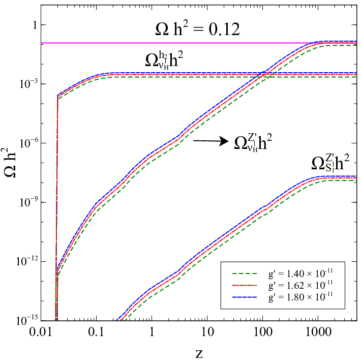


In the left and right panels of Fig. 10, we show the variation of relic density contributions of the two component DM scenario for different values of and , respectively. The top panels stand for the decay contribution while the bottom ones stand for the annihilation contribution. Again from these figures, one can easily conclude that FIMP relic density contributions are inversely proportional to the mediator mass, as illustrated in left panels, and directly proportional to coupling strength as shown in right panels. We have discussed these features before in section 3.


4.2 Region II:
In discussed above, for (region I), the total relic density is dominated by mediated diagrams. Now we turn to the region II, where and decays to pair is kinematically forbidden, and consequently, production is dominated. Therefore in region II, a major portion of our two DM candidates, and , is produced almost independently from the and mediated processes, respectively. In other words, by fixing , and at certain values to get a significant contribution from , one can obtain a relevant contribution independently by changing within keV range. This possibility did not exist in region I because both and are produced dominantly via and therefore have the same number density. The only way to have comparable contribution from both in region I would be to raise the mass of to the GeV range. However, this is untenable since that will spoil the inverse seesaw mechanism scenario for generating light neutrino masses MohapatraIS1; Mohapatra:1986bd; Khalil:2010iu; GonzalezGarcia:1988rw. In region II this lacuna is remedied since here and are produced independently - while are dominantly produced from , are produced from .
In Fig. 11, for two suitably chosen sets of BLSMIS parameters ( GeV ( GeV), GeV ( GeV), keV ( keV), rad, , TeV, and ), we show variation of decay and annihilation contributions to the relic density of and , as a function of . In the figure, green dashed-dotted and red dashed-double-dotted lines correspond to the relic density contributions ( and ), respectively, while blue dashed line corresponds to relic density contribution from decay of (). From the figure, it is clearly seen that has a relevant relic density contribution, unlike the situation in region I. Note that for a larger mass ( keV), the contribution to the total relic density even starts to be the dominant one, as seen in the right panel of Fig. 11.
5 Conclusion
In this work we studied two beyond SM problems, viz., the non-zero neutrino masses and the existence of the DM. In studying the tiny neutrino masses, we followed the inverse seesaw mechanism within the extension of the SM (BLSMIS). Six SM singlet fermions were introduced for inverse seesaw mechanism to work and three more singlet fermions (with mass of order keV) were added to cancel the gauge anomaly. The lightest of these additional fermionic states, , can be a WDM, being odd under a discrete symmetry. We studied as a FIMP WDM and showed that it could be produced via the freeze-in mechanism from the decay of the extra neutral gauge boson and the on-shell annihilation processes mediated by . We showed that the relative contributions to the DM relic density from both the decay and the on-shell annihilation processes are more or less equal. We scanned over the relevant BLSMIS parameters by imposing the Planck constraint of the DM relic density and showed that a large portion of the parameter space gives a small contribution to the DM relic density. Therefore, we studied a two component FIMP DM as a possible scenario in the BLSMIS to get an extra contribution to the DM relic density. In this scenario, the lightest heavy RH neutrino, , can contribute to the DM relic density as an independent DM component (with mass of order GeV). For , we showed that the production of as a DM candidate through the mediator has the dominant contribution to the total DM relic density. On the other hand for , the mediated processes will contribute dominantly to production while mediated processes will contribute dominantly to production. We emphasized that in this region both FIMP candidates ( and ) can contribute to the total DM relic density.
Acknowledgements
The authors would like to thank the Department of Atomic Energy Neutrino Project of Harish-Chandra Research Institute (HRI). We also acknowledge the HRI cluster computing facility (http://www.hri.res.in/cluster/). This project has received funding from the European Union’s Horizon 2020 research and innovation programme InvisiblesPlus RISE under the Marie Sklodowska-Curie grant agreement No. 690575 and No. 674896. The authors would like to thank Abhass Kumar for fruitful discussions.
Appendix
Appendix A Analytical expression of the collision terms
For any generic process (where ), the collision term takes the following form Kolb:1990vq; Gondolo:1990dk,
| (42) | |||||
From Eq. (29), we can see that the Boltzmann equation which determine the distribution function of the extra gauge boson contains two collision terms one is for its production and the another one is for its decay. The expression for the two collision terms are described below.
- •
: Collision term for the gauge boson decay takes the following form after using the Eq. (42),
(43) where and + . Expression for the each decay terms are as follows,
(44) where refers to the SM fermions and . and are the corresponding color and electric charges, respectively. for and for .
- •
: The expression for this collision term where () decays to pair takes the following form,
(45) where
(46) - •
Relevant partial decay widths of the scalars ():
(47) (48) where , , and the coupling is defined in Eq. (37).
References
- (1) F. Zwicky, Helv. Phys. Acta 6, 110 (1933) [Gen. Rel. Grav. 41, 207 (2009)].
- (2) V. C. Rubin and W. K. Ford, Jr., Astrophys. J. 159, 379 (1970).
- (3) D. Clowe, M. Bradac, A. H. Gonzalez, M. Markevitch, S. W. Randall, C. Jones and D. Zaritsky, Astrophys. J. 648, L109 (2006) [astro-ph/0608407].
- (4) P. A. R. Ade et al. [Planck Collaboration], Astron. Astrophys. 594, A13 (2016) [arXiv:1502.01589 [astro-ph.CO]].
- (5) P. Gondolo and G. Gelmini, Nucl. Phys. B 360, 145 (1991).
- (6) M. Srednicki, R. Watkins and K. A. Olive, Nucl. Phys. B 310, 693 (1988).
- (7) E. Aprile et al. [XENON Collaboration], Phys. Rev. Lett. 121, no. 11, 111302 (2018) [arXiv:1805.12562 [astro-ph.CO]].
- (8) A. Tan et al. [PandaX-II Collaboration], Phys. Rev. Lett. 117, no. 12, 121303 (2016) [arXiv:1607.07400 [hep-ex]].
- (9) D. S. Akerib et al. [LUX Collaboration], Phys. Rev. Lett. 118, no. 2, 021303 (2017) [arXiv:1608.07648 [astro-ph.CO]].
- (10) C. Amole et al. [PICO Collaboration], Phys. Rev. Lett. 118, no. 25, 251301 (2017) [arXiv:1702.07666 [astro-ph.CO]].
- (11) E. Aprile et al. [XENON Collaboration], Phys. Rev. Lett. 122, no. 14, 141301 (2019) [arXiv:1902.03234 [astro-ph.CO]].
- (12) M. L. Ahnen et al. [MAGIC and Fermi-LAT Collaborations], JCAP 1602, no. 02, 039 (2016) [arXiv:1601.06590 [astro-ph.HE]].
- (13) H. Abdallah et al. [H.E.S.S. Collaboration], Phys. Rev. Lett. 117, no. 11, 111301 (2016) [arXiv:1607.08142 [astro-ph.HE]].
- (14) G. Giesen, M. Boudaud, Y. Génolini, V. Poulin, M. Cirelli, P. Salati and P. D. Serpico, JCAP 1509, no. 09, 023 (2015) [arXiv:1504.04276 [astro-ph.HE]].
- (15) A. Drukier and L. Stodolsky, Phys. Rev. D 30, 2295 (1984).
- (16) P. Cushman et al., arXiv:1310.8327 [hep-ex].
- (17) L. J. Hall, K. Jedamzik, J. March-Russell and S. M. West, JHEP 1003, 080 (2010) [arXiv:0911.1120 [hep-ph]].
- (18) J. König, A. Merle and M. Totzauer, JCAP 1611, no. 11, 038 (2016) [arXiv:1609.01289 [hep-ph]].
- (19) A. Biswas and A. Gupta, JCAP 1609, no. 09, 044 (2016) Addendum: [JCAP 1705, no. 05, A01 (2017)] [arXiv:1607.01469 [hep-ph]].
- (20) A. Biswas and A. Gupta, JCAP 1703, no. 03, 033 (2017) Addendum: [JCAP 1705, no. 05, A02 (2017)] [arXiv:1612.02793 [hep-ph]].
- (21) A. Biswas, S. Choubey and S. Khan, JHEP 1702, 123 (2017) [arXiv:1612.03067 [hep-ph]].
- (22) A. Biswas, S. Choubey and S. Khan, Eur. Phys. J. C 77, no. 12, 875 (2017) [arXiv:1704.00819 [hep-ph]].
- (23) A. Biswas, S. Choubey, L. Covi and S. Khan, JCAP 1802, no. 02, 002 (2018) [arXiv:1711.00553 [hep-ph]].
- (24) K. Kaneta, Z. Kang and H. S. Lee, JHEP 1702, 031 (2017) [arXiv:1606.09317 [hep-ph]].
- (25) A. Caputo, P. Hernandez and N. Rius, arXiv:1807.03309 [hep-ph].
- (26) C. L. Cowan, F. Reines, F. B. Harrison, H. W. Kruse and A. D. McGuire, Science 124, 103 (1956).
- (27) Y. Fukuda et al. [Super-Kamiokande Collaboration], Phys. Rev. Lett. 81, 1562 (1998) [hep-ex/9807003].
- (28) Q. R. Ahmad et al. [SNO Collaboration], Phys. Rev. Lett. 89, 011301 (2002) [nucl-ex/0204008].
- (29) K. Eguchi et al. [KamLAND Collaboration], Phys. Rev. Lett. 90, 021802 (2003) [hep-ex/0212021].
- (30) F. P. An et al. [Daya Bay Collaboration], Phys. Rev. Lett. 116, no. 6, 061801 (2016) [arXiv:1508.04233 [hep-ex]].
- (31) J. H. Choi et al. [RENO Collaboration], Phys. Rev. Lett. 116, no. 21, 211801 (2016) [arXiv:1511.05849 [hep-ex]].
- (32) Y. Abe et al. [Double Chooz Collaboration], JHEP 1410, 086 (2014) Erratum: [JHEP 1502, 074 (2015)] [arXiv:1406.7763 [hep-ex]].
- (33) K. Abe et al. [T2K Collaboration], Phys. Rev. D 91, no. 7, 072010 (2015) [arXiv:1502.01550 [hep-ex]].
- (34) M. Ravonel Salzgeber [T2K Collaboration], arXiv:1508.06153 [hep-ex].
- (35) P. Adamson et al. [NOvA Collaboration], Phys. Rev. Lett. 116, no. 15, 151806 (2016) [arXiv:1601.05022 [hep-ex]].
- (36) P. Adamson et al. [NOvA Collaboration], Phys. Rev. D 93, no. 5, 051104 (2016) [arXiv:1601.05037 [hep-ex]].
- (37) S. Khalil, J. Phys. G G 35, 055001 (2008) [hep-ph/0611205].
- (38) W. Emam and S. Khalil, Eur. Phys. J. C 55, 625 (2007) [arXiv:0704.1395 [hep-ph]].
- (39) S. Blanchet, Z. Chacko, S. S. Granor and R. N. Mohapatra, Phys. Rev. D 82, 076008 (2010) [arXiv:0904.2174 [hep-ph]].
- (40) L. Basso, A. Belyaev, S. Moretti and C. H. Shepherd-Themistocleous, Phys. Rev. D 80, 055030 (2009) [arXiv:0812.4313 [hep-ph]].
- (41) K. Huitu, S. Khalil, H. Okada and S. K. Rai, Phys. Rev. Lett. 101, 181802 (2008) [arXiv:0803.2799 [hep-ph]].
- (42) R. N. Mohapatra and R. E. Marshak, Phys. Rev. Lett. 44, 1316 (1980) [Erratum-ibid. 44, 1643 (1980)].
- (43) R. E. Marshak and R. N. Mohapatra, Phys. Lett. B 91, 222 (1980).
- (44) C. Wetterich, Nucl. Phys. B 187, 343 (1981).
- (45) A. Masiero, J. F. Nieves and T. Yanagida, Phys. Lett. B 116, 11 (1982).
- (46) R. N. Mohapatra and G. Senjanovic, Phys. Rev. D 27, 254 (1983).
- (47) W. Buchmuller, C. Greub and P. Minkowski, Phys. Lett. B 267, 395 (1991).
- (48) M. Abbas and S. Khalil, JHEP 0804, 056 (2008) [arXiv:0707.0841 [hep-ph]].
- (49) S. Khalil, Phys. Rev. D 82, 077702 (2010) [arXiv:1004.0013 [hep-ph]].
- (50) R. N. Mohapatra, Phys. Rev. Lett. 56, 561 (1986).
- (51) R. N. Mohapatra and J. W. F. Valle, Phys. Rev. D 34, 1642 (1986).
- (52) M. C. Gonzalez-Garcia and J. W. F. Valle, Phys. Lett. B 216, 360 (1989).
- (53) G. ’t Hooft, NATO Sci. Ser. B 59, 135 (1980).
- (54) H. Pagels and J. R. Primack, Phys. Rev. Lett. 48, 223 (1982).
- (55) P. J. E. Peebles, Astrophys. J. 258, 415 (1982).
- (56) J. R. Bond, A. S. Szalay and M. S. Turner, Phys. Rev. Lett. 48, 1636 (1982).
- (57) K. A. Olive and M. S. Turner, Phys. Rev. D 25, 213 (1982).
- (58) A. El-Zant, S. Khalil and A. Sil, Phys. Rev. D 91, no. 3, 035030 (2015) [arXiv:1308.0836 [hep-ph]].
- (59) A. Boyarsky, O. Ruchayskiy and M. Shaposhnikov, Ann. Rev. Nucl. Part. Sci. 59, 191 (2009) [arXiv:0901.0011 [hep-ph]].
- (60) M. Re Fiorentin, V. Niro and N. Fornengo, JHEP 1611, 022 (2016) [arXiv:1606.04445 [hep-ph]].
- (61) P. Di Bari, P. O. Ludl and S. Palomares-Ruiz, JCAP 1611, no. 11, 044 (2016) [arXiv:1606.06238 [hep-ph]].
- (62) B. Holdom, Phys. Lett. B 166, 196 (1986).
- (63) P. H. Chankowski, S. Pokorski and J. Wagner, Eur. Phys. J. C 47, 187 (2006) [hep-ph/0601097].
- (64) M. E. Krauss, B. O’Leary, W. Porod and F. Staub, Phys. Rev. D 86, 055017 (2012) [arXiv:1206.3513 [hep-ph]].
- (65) P. Abreu et al. [DELPHI Collaboration], Z. Phys. C 65, 603 (1995).
- (66) J. Alcaraz et al. [ALEPH and DELPHI and L3 and OPAL Collaborations and LEP Electroweak Working Group], hep-ex/0612034.
- (67) J. Erler, P. Langacker, S. Munir and E. Rojas, JHEP 0908, 017 (2009) [arXiv:0906.2435 [hep-ph]].
- (68) G. Cacciapaglia, C. Csaki, G. Marandella and A. Strumia, Phys. Rev. D 74, 033011 (2006) [hep-ph/0604111].
- (69) M. Carena, A. Daleo, B. A. Dobrescu and T. M. P. Tait, Phys. Rev. D 70, 093009 (2004) [hep-ph/0408098].
- (70) W. Abdallah, A. Awad, S. Khalil and H. Okada, Eur. Phys. J. C 72, 2108 (2012) [arXiv:1105.1047 [hep-ph]].
- (71) E. Ma, Phys. Rev. D 80, 013013 (2009) [arXiv:0904.4450 [hep-ph]].
- (72) A. A. Abdelalim, A. Hammad and S. Khalil, Phys. Rev. D 90, no. 11, 115015 (2014) [arXiv:1405.7550 [hep-ph]].
- (73) P. Bandyopadhyay, E. J. Chun, H. Okada and J. C. Park, JHEP 1301, 079 (2013) [arXiv:1209.4803 [hep-ph]].
- (74) W. Abdallah, D. Delepine and S. Khalil, Phys. Lett. B 725, 361 (2013) [arXiv:1205.1503 [hep-ph]].
- (75) D. Hooper, F. S. Queiroz and N. Y. Gnedin, Phys. Rev. D 85, 063513 (2012) [arXiv:1111.6599 [astro-ph.CO]].
- (76) G. Aad et al. [ATLAS Collaboration], Phys. Lett. B 716, 1 (2012) [arXiv:1207.7214 [hep-ex]].
- (77) S. Chatrchyan et al. [CMS Collaboration], Phys. Lett. B 716, 30 (2012) [arXiv:1207.7235 [hep-ex]].
- (78) L. Basso, S. Moretti and G. M. Pruna, Phys. Rev. D 82, 055018 (2010) [arXiv:1004.3039 [hep-ph]].
- (79) F. Staub, Comput. Phys. Commun. 185 (2014) 1773 [arXiv:1309.7223 [hep-ph]].
- (80) F. Staub, Comput. Phys. Commun. 181 (2010) 1077 [arXiv:0909.2863 [hep-ph]].
- (81) F. Staub, arXiv:0806.0538 [hep-ph].
- (82) W. Porod and F. Staub, Comput. Phys. Commun. 183 (2012) 2458 [arXiv:1104.1573 [hep-ph]].
- (83) M. Drewes et al., JCAP 1701, no. 01, 025 (2017) [arXiv:1602.04816 [hep-ph]].
- (84) N. Bernal, M. Heikinheimo, T. Tenkanen, K. Tuominen and V. Vaskonen, Int. J. Mod. Phys. A 32, no. 27, 1730023 (2017) [arXiv:1706.07442 [hep-ph]].
- (85) A. Abada, G. Arcadi and M. Lucente, JCAP 1410, 001 (2014) [arXiv:1406.6556 [hep-ph]].
- (86) G. Arcadi and L. Covi, JCAP 1308, 005 (2013) [arXiv:1305.6587 [hep-ph]].
- (87) E. W. Kolb and M. S. Turner, Front. Phys. 69, 1 (1990).
- (88) G. Bélanger, F. Boudjema, A. Goudelis, A. Pukhov and B. Zaldivar, Comput. Phys. Commun. 231, 173 (2018) [arXiv:1801.03509 [hep-ph]].
- (89) J. Edsjo and P. Gondolo, Phys. Rev. D 56, 1879 (1997) [hep-ph/9704361].
- (90) S. Iso, N. Okada and Y. Orikasa, Phys. Rev. D 83, 093011 (2011) [arXiv:1011.4769 [hep-ph]].
- (91) G. Aad et al. [ATLAS and CMS Collaborations], JHEP 1608, 045 (2016) [arXiv:1606.02266 [hep-ex]].