Interval Algorithm for Random Number Generation: Information Spectrum Approach Thanks: A part of this paper is submitted for possible presentation at 2019 IEEE Information Theory Workshop.

Shun Watanabe Te Sun Han

Abstract

The problem of exactly generating a general random process (target process) by using another general random process (coin process) is studied. The performance of the interval algorithm, introduced by Han and Hoshi, is analyzed from the perspective of information spectrum approach. When either the coin process or the target process has one point spectrum, the asymptotic optimality of the interval algorithm among any random number generation algorithms is proved, which demonstrates utility of the interval algorithm beyond the ergodic process. Furthermore, the feasibility condition of exact random number generation is also elucidated. Finally, the obtained general results are illustrated by the case of generating a Markov process from another Markov process.

I Introduction

We revisit the problem of exactly generating a random process, termed target process, from another random process, termed coin process. This problem has a long history. In a seminal paper [35], von Neumann introduced an algorithm to generate the independently identically distributed (i.i.d.) binary unbiased process from an i.i.d. binary biased process. Subsequently, his result was extended and refined in various directions [28, 14, 7, 4, 25]. On the other hand, Knuth and Yao [15] studied the problem of generating an arbitrary target process using i.i.d. unbiased coin process. Later, the problem of generating an arbitrary target process from an arbitrary coin process was studied by various researchers [27, 1]. For instance, by generalizing the approach in [15], Abrahams proposed an algorithm to generate an arbitrary target process from an i.i.d. biased (not necessarily binary) coin process [1]; however, this algorithm is only applicable to the algebraic coin, i.e., the case where the probabilities of coin random variable is described by the root of a polynomial equation. In this paper, we focus on the interval algorithm proposed in [10]. The interval algorithm is constructive, and it can be applied to any coin/target processes that may have memory and may not be stationary nor ergodic. Thus, it is of interest to identify under what circumstances the interval algorithm has the optimal performance. In fact, despite simplicity of the algorithm, performance analysis of the interval algorithm is not straightforward.

When the coin process is i.i.d., Han and Hoshi have shown that the interval algorithm asymptotically attains the optimal performance among any random number generation algorithm [10]; more precisely, they have shown that the average stopping time of the coin process, i.e., the average number of coin tosses, of the interval algorithm converges to the fundamental limit, which is given by the ratio between the entropy rates of the coin and target processes. Using representation of real numbers, Oohama refined Han and Hoshi’s performance analysis of the interval algorithm [23, 24].

For i.i.d. coin processes, the performance of the interval algorithm is fairly well understood. However, in practice, it is also desirable to use a coin process that has a memory, such as the Markov process. When the coin process is Markov, the performance analysis of the interval algorithm become intractable. In fact, even though performance analysis of the interval algorithm for the Markov coin process was conducted in [10, 24], the analyses there do not guarantee asymptotic optimality. One of the motivations of this paper is to elucidate the performance of the interval algorithm when the coin process is Markov.

On the other hand, Uyematsu and Kanaya studied the overflow probability of the stopping time of the interval algorithm [31, 32]. In [32], they derived an exponential convergence rate of the overflow probability of the stopping time for i.i.d. processes. In [31], using the sample path approach [29], they derived almost sure convergence results on the stopping time for general coin/target processes; however, since their characterization is in terms of the quantities defined for sample path [20], it is not immediately clear how to evaluate those quantities other than ergodic processes. Moreover, they only analyzed the interval algorithm and did not discuss the optimality of the interval algorithm among other random number generation algorithms. Even though the almost sure convergence analysis is of theoretical importance, the authors believe that the average performance analysis is preferable in practice since it provides more insights on the finite length performance along the way of deriving asymptotic results. It should be also pointed out that the almost sure convergence of stopping time does not immediately provide performance guarantee of the average stopping time (cf. Remark 14).

As a related problem to the above, the problem of random number generation with approximation error has been extensively studied in the past few decades [11, 34, 21, 8, 12, 2, 22, 17]. In such a direction of research, the information spectrum approach introduced in [11, 9] is successfully used to derive fairly general results.

In this paper, we apply the information spectrum approach to the problem of exactly generating a random process by another random process. First, we derive a converse bound on the overflow probability of the stopping time for any random number generation algorithms. Second, we derive an achievability bound on the overflow probability of the stopping time that can be attained by the interval algorithm. Using these bounds, we examine the asymptotic optimality of the interval algorithm for general coin/target processes. For the criterion of the overflow probability of the stopping time, when either the coin or the target process has one point spectrum, the optimality of the interval algorithm among any random number generation algorithms is proved. For the average stopping time criterion, when the coin process has one point spectrum with an additional mild condition, the optimality of the interval algorithm among any random number generation algorithms is proved. These results demonstrate the utility of the interval algorithm for non-stationary and/or non-ergodic processes. As a side result, we also elucidate the condition that exact random number generation is possible. Finally, we illustrate the obtained general results by the case of Markov coin/target processes.

The rest of the paper is organized as follows. In Section II, we describe the problem formulation and derive a converse bound for any random number generation algorithm. In Section III, we derive an achievability bound for the interval algorithm. In Section IV, we conduct the asymptotic analysis. In Section V, we mention the connection between the variable-length random number generation and the fixed-length random number generation. We close the paper with discussion in Section VI.

Notation

Throughout the paper, random variables (eg. $X$ ) and their realizations (eg. $x$ ) are denoted by capital and lower case letters, respectively. The ranges of random variables are denoted by the respective calligraphic letters (eg. ${\cal X}$ ). The probability distribution of random variable $X$ is denoted by $P_{X}$ . Similarly, $X^{n}=(X_{1},\ldots,X_{n})$ and $x^{n}=(x_{1},\ldots,x_{n})$ denote, respectively, a random vector and its realization in the $n$ th Cartesian product ${\cal X}^{n}$ of ${\cal X}$ . We use the standard notations for information measures [5], such as the entropy $H(X)$ , the min-entropy $H_{\min}(X)=\min_{x}\log\frac{1}{P_{X}(x)}$ , and the binary entropy function $h(t)=t\log(1/t)+(1-t)\log(1/(1-t))$ for $0\leq t\leq 1$ . For a random process $\bm{X}=\{X^{n}\}_{n=1}^{\infty}$ , the spectral sup-entropy and the spectral inf-entropy are denoted by

\displaystyle\overline{H}(\bm{X}):=\inf\bigg\{\lambda:\lim_{n\to\infty}\Pr\bigg(\frac{1}{n}\log\frac{1}{P_{X^{n}}(X^{n})}\geq\lambda\bigg)=0\bigg\}

(1)

and

\displaystyle\underline{H}(\bm{X}):=\sup\bigg\{\lambda:\lim_{n\to\infty}\Pr\bigg(\frac{1}{n}\log\frac{1}{P_{X^{n}}(X^{n})}\leq\lambda\bigg)=0\bigg\},

(2)

respectively [9]. The sup-entropy rate is denoted by

\displaystyle H(\bm{X}):=\limsup_{n\to\infty}\frac{1}{n}H(X^{n}),

(3)

and it coincides with the entropy rate if the limit exists. The base of $\log$ and $\exp$ is $2$ and the natural logarithm is denoted by $\ln$ .

II Problem Formulation and Basic Results

In this section, we describe the problem formulation of random number generation with variable length coin tossing. Let $\bm{X}=\{X^{m}=(X_{1},\ldots,X_{m})\}_{m=1}^{\infty}$ be a random process taking values in a finite set ${\cal X}=\{1,\ldots,M\}$ , and let $\bm{Y}=\{Y^{n}=(Y_{1},\ldots,Y_{n})\}_{n=1}^{\infty}$ be a random process taking values in a finite set ${\cal Y}=\{1,\ldots,N\}$ . Unless otherwise stated, the distributions $P_{X^{m}}$ and $P_{Y^{n}}$ of the processes can be arbitrary as long as they are consistent over time; i.e.,

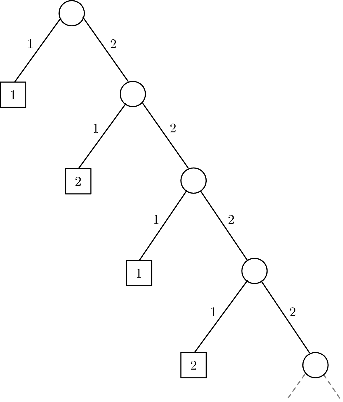
\displaystyle\sum_{x_{m+1}}P_{X^{m+1}}(x^{m},x_{m+1})=P_{X^{m}}(x^{m})

for every $m$ and $x^{m}\in{\cal X}^{m}$ , and similarly for $P_{Y^{n}}$ . We shall consider the problem of random number generation to simulate the sequence of random variables $Y^{n}$ using outputs from the sequence of random variable $X^{m}$ ; the former is referred to as target process and the latter is referred to as coin process. Specifically, an algorithm of random number generation with variable length coin tossing is described by a full $M$ -ary tree of possibly infinite depth (see Example 1 below); that is, it is described by a deterministic function

\displaystyle\phi:\bigcup_{i=0}^{\infty}{\cal X}^{i}\to\{\bot\}\cup{\cal Y}^{n}

(4)

such that $\phi(x^{i})\in{\cal Y}^{n}$ if $x^{i}$ corresponds to a leaf and $\phi(x^{i})=\bot$ otherwise, where $\bot$ is the null sequence and ${\cal X}^{0}=\{\bot\}$ . Let ${\cal L}_{\phi}$ be the set of all leaves, i.e.,

\displaystyle{\cal L}_{\phi}:=\bigg\{s\in\bigcup_{i=0}^{\infty}{\cal X}^{i}:\phi(s)\in{\cal Y}^{n}\mbox{ and for all proper prefix }s^{\prime}\mbox{ of }s,~\phi(s^{\prime})=\bot\bigg\}.

For a leaf $s=(x_{1},\ldots,x_{i})\in{\cal L}_{\phi}$ , its depth $i$ is denoted by $|s|$ .

For a given infinite sequence $x_{1},x_{2},\ldots$ , starting with $i=0$ , we output a symbol in ${\cal Y}^{n}$ by the following algorithm:

1.

If $\phi(x^{i})$ is in ${\cal Y}^{n}$ , output $\phi(x^{i})$ and terminate;
2.

Set $i=i+1$ , and go back to Step 1.

For performance analysis, it is convenient to consider the output of the algorithm for an input sequence of finite length. By an abuse of notation, we denote the output of the above algorithm for a sequence $x^{m}$ by $\phi(x^{m})$ , i.e., $\phi(x^{m})=y^{n}$ if the algorithm terminates with output $\phi(x^{i})=y^{n}$ for some $i\leq m$ , and $\phi(x^{m})=\bot$ otherwise. The stopping time of the algorithm, i.e., the minimum integer $m\geq 0$ such that $\phi(X^{m})\in{\cal Y}^{n}$ , is denoted by $T$ ; note that the stopping time $T$ is the random variable that is induced by the algorithm and the coin process $\bm{X}$ . For any fixed length $n$ of the target process, we require that the probability law of the output of the algorithm coincides with $P_{Y^{n}}$ exactly as $m\to\infty$ , i.e.,

\displaystyle\sum_{s\in{\cal L}_{\phi}:\atop\phi(s)=y^{n}}P_{X^{|s|}}(s)=\lim_{m\to\infty}\Pr(\phi(X^{m})=y^{n})=P_{Y^{n}}(y^{n})

(5)

for every $y^{n}\in{\cal Y}^{n}$ .

Note that the algorithm described as in (4) outputs sequence $y^{n}\in{\cal Y}^{n}$ of length $n$ collectively. Practically, it is also important to consider an algorithm that outputs symbol $y_{j}$ whenever it is ready; such an algorithm is termed a sequential algorithm. We will consider a sequential version of the interval algorithm in the next section. It should be noted that, for a given sequential algorithm, we can describe that algorithm in the form of (4) by pooling $y_{1},\ldots,y_{n-1}$ until $y_{n}$ is ready to be output. Thus, the converse bound to be described later in this section is also valid for sequential algorithms.

Let us illustrate the problem formulation by the following simple example.

Example 1 ([5])

Let us consider generation of one symbol, i.e., $n=1$ , of random variable with distribution $P_{Y}=(2/3,1/3)$ using the i.i.d. sequence $\{X^{m}\}_{m=1}^{\infty}$ of unbiased binary random variables. For this example, by noting the binary expansions

	$\displaystyle\frac{2}{3}$	$\displaystyle=\sum_{i=1}^{\infty}2^{-(2i-1)},$
	$\displaystyle\frac{1}{3}$	$\displaystyle=\sum_{i=1}^{\infty}2^{-2i},$

we can construct an algorithm with the tree described in Fig. 1.

Refer to caption — Fig. 1: A description of algorithm tree in Example 1. The label $1$ or $2$ of each edge indicates the outcome of coin random variable $X_{i}$ . The circle node at depth $i$ indicates that the algorithm does not terminate when $X^{i}$ is observed; the square node at depth $i$ indicates that the algorithm terminates with the output labeled in that square node.

When the coin process is i.i.d. with common distribution $P_{X}$ , there is a useful lower bound on the expected stopping time (cf. [10, Eq. (2.4)]):

\displaystyle\mathbb{E}[T]\geq\frac{H(Y^{n})}{H(X)}.

Since this lower bound is not available for general coin processes, the following lower bound on the overflow probability of the stopping time $\Pr(T>m)$ is of importance in the latter sections; note that this lower bound is reminiscent of [9, Lemma 2.1.2].

Theorem 2

For arbitrary random number generation algorithm satisfying (5) and integer $m\geq 0$ , the overflow probability of the stopping time satisfies

	$\displaystyle\Pr(T>m)$	$\displaystyle\geq P_{Y^{n}}({\cal T}_{n}^{c}(\tau))-P_{X^{m}}({\cal S}_{m}(\lambda))-2^{-\tau+\lambda}$		(6)
		$\displaystyle=P_{X^{m}}({\cal S}_{m}^{c}(\lambda))-P_{Y^{n}}({\cal T}_{n}(\tau))-2^{-\tau+\lambda}$		(7)

for arbitrary real numbers $\tau,\lambda\geq 0$ , where

	$\displaystyle{\cal S}_{m}(\lambda)$	$\displaystyle:=\bigg\{x^{m}\in{\cal X}^{m}:\log\frac{1}{P_{X^{m}}(x^{m})}\geq\lambda\bigg\},$		(8)
	$\displaystyle{\cal T}_{n}(\tau)$	$\displaystyle:=\bigg\{y^{n}\in{\cal Y}^{n}:\log\frac{1}{P_{Y^{n}}(y^{n})}\leq\tau\bigg\}.$		(9)

Proof.

Without loss of generality, we can assume that there is no leaf $s\in{\cal L}_{\phi}$ such that $|s|<m$ ; otherwise, we can expand that leaf to depth $m$ without changing the overflow probability $\Pr(T>m)$ . Thus, we assume this assumption is satisfied in the rest of the proof.

Let

\displaystyle{\cal B}:=\big\{s\in{\cal L}_{\phi}:|s|=m\big\}.

Then, we can write

\displaystyle\Pr(T>m)=\sum_{s\in{\cal B}^{c}}P_{X^{|s|}}(s),

where ${\cal B}^{c}={\cal L}_{\phi}\backslash{\cal B}$ . Let

\displaystyle{\cal C}:=\big\{s\in{\cal L}_{\phi}:\phi(s)\in{\cal T}_{n}^{c}(\tau)\big\}.

Then, we have

$\displaystyle P_{Y^{n}}({\cal T}_{n}^{c}(\tau))$	$\displaystyle=\sum_{s\in{\cal C}}P_{X^{\|s\|}}(s)$
	$\displaystyle=\sum_{s\in{\cal B}\cap{\cal C}}P_{X^{m}}(s)+\sum_{s\in{\cal B}^{c}\cap{\cal C}}P_{X^{\|s\|}}(s)$
	$\displaystyle\leq\sum_{s\in{\cal B}\cap{\cal C}}P_{X^{m}}(s)+\sum_{s\in{\cal B}^{c}}P_{X^{\|s\|}}(s)$
	$\displaystyle=\sum_{s\in{\cal B}\cap{\cal C}}P_{X^{m}}(s)+\Pr(T>m),$	(10)

where the first identity follows from (5). Furthermore, we have

$\displaystyle\sum_{s\in{\cal B}\cap{\cal C}}P_{X^{m}}(s)$	$\displaystyle=\sum_{s\in{\cal B}\cap{\cal C}\cap{\cal S}_{m}(\lambda)}P_{X^{m}}(s)+\sum_{s\in{\cal B}\cap{\cal C}\cap{\cal S}_{m}^{c}(\lambda)}P_{X^{m}}(s)$
	$\displaystyle\leq P_{X^{m}}({\cal S}_{m}(\lambda))+\sum_{s\in{\cal B}\cap{\cal C}\cap{\cal S}_{m}^{c}(\lambda)}P_{X^{m}}(s)$
	$\displaystyle\leq P_{X^{m}}({\cal S}_{m}(\lambda))+\sum_{s\in{\cal B}\cap{\cal C}\cap{\cal S}_{m}^{c}(\lambda)}P_{Y^{n}}(\phi(s))$
	$\displaystyle\leq P_{X^{m}}({\cal S}_{m}(\lambda))+\sum_{s\in{\cal B}\cap{\cal C}\cap{\cal S}_{m}^{c}(\lambda)}2^{-\tau}$
	$\displaystyle\leq P_{X^{m}}({\cal S}_{m}(\lambda))+2^{-\tau+\lambda},$	(11)

where the second inequality follows from $\phi(s)\in{\cal Y}^{n}$ for $s\in{\cal C}$ , the third inequality follows from $\phi(s)\in{\cal T}^{c}_{n}(\tau)$ for $s\in{\cal C}$ , and the last inequality follows from the bound $|{\cal S}_{m}^{c}(\lambda)|\leq 2^{\lambda}$ . By combining (10) and (11), we obtain (6); then, (7) follows from (6). ∎

III Performance of Interval Algorithm

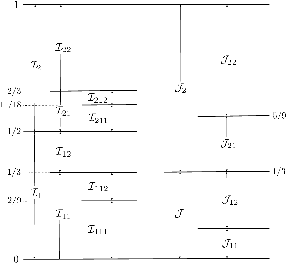
First, we review a sequential version of the interval algorithm.¹¹ 1 Unlike the interval algorithm in [10], we output each symbol of the target process sequentially; however, there is no difference in performance analyses. In the algorithm, we sequentially update intervals

	$\displaystyle{\cal I}_{s}$	$\displaystyle:=[\underline{\alpha}_{s},\overline{\alpha}_{s}),$
	$\displaystyle{\cal J}_{t}$	$\displaystyle:=[\underline{\beta}_{t},\overline{\beta}_{t})$

induced by coin process and target process, respectively. For the null sequence $s=t=\bot$ , we initially set $\underline{\alpha}_{s}=\underline{\beta}_{t}=0$ and $\overline{\alpha}_{s}=\overline{\beta}_{t}=1$ . For a given sequence $s\in{\cal X}^{i}$ and $x\in{\cal X}$ , the interval of coin process is updated by

	$\displaystyle\underline{\alpha}_{sx}$	$\displaystyle:=\underline{\alpha}_{s}+(\overline{\alpha}_{s}-\underline{\alpha}_{s})P_{(x-1)\|s},$
	$\displaystyle\overline{\alpha}_{sx}$	$\displaystyle:=\underline{\alpha}_{s}+(\overline{\alpha}_{s}-\underline{\alpha}_{s})P_{x\|s},$

where

\displaystyle P_{x|s}:=\sum_{k=1}^{x}P_{X_{i+1}|X^{i}}(k|s)

for $x\in{\cal X}$ and $P_{0|s}=0$ . Similarly, for a given sequence $t\in{\cal Y}^{j}$ and $y\in{\cal Y}$ , the interval of target process is updated by

	$\displaystyle\underline{\beta}_{ty}$	$\displaystyle:=\underline{\beta}_{t}+(\overline{\beta}_{t}-\underline{\beta}_{t})Q_{(y-1)\|t},$
	$\displaystyle\overline{\beta}_{ty}$	$\displaystyle:=\underline{\beta}_{t}+(\overline{\beta}_{t}-\underline{\beta}_{t})Q_{y\|t},$

where

\displaystyle Q_{y|t}:=\sum_{k=1}^{y}P_{Y_{j+1}|Y^{j}}(k|t)

for $y\in{\cal Y}$ and $Q_{0|t}=0$ . Using these intervals, the algorithm proceeds as follows:

1.

Set $s=t=\bot$ , $i=0$ , and $j=1$ .
2.

If $[\underline{\alpha}_{s},\overline{\alpha}_{s})\subseteq[\underline{\beta}_{ty},\overline{\beta}_{ty})$ for some $y\in{\cal Y}$ , then output $y_{j}=y$ and go to Step 3; otherwise, set $i=i+1$ , $s=sx_{i}$ , and repeat Step 2 again.
3.

If $j=n$ , terminates; otherwise, set $t=ty_{j}$ , $j=j+1$ , and go to Step 2.

The following example illustrates a behavior of the interval algorithm for converting a Markov process to an i.i.d. process.

Example 3

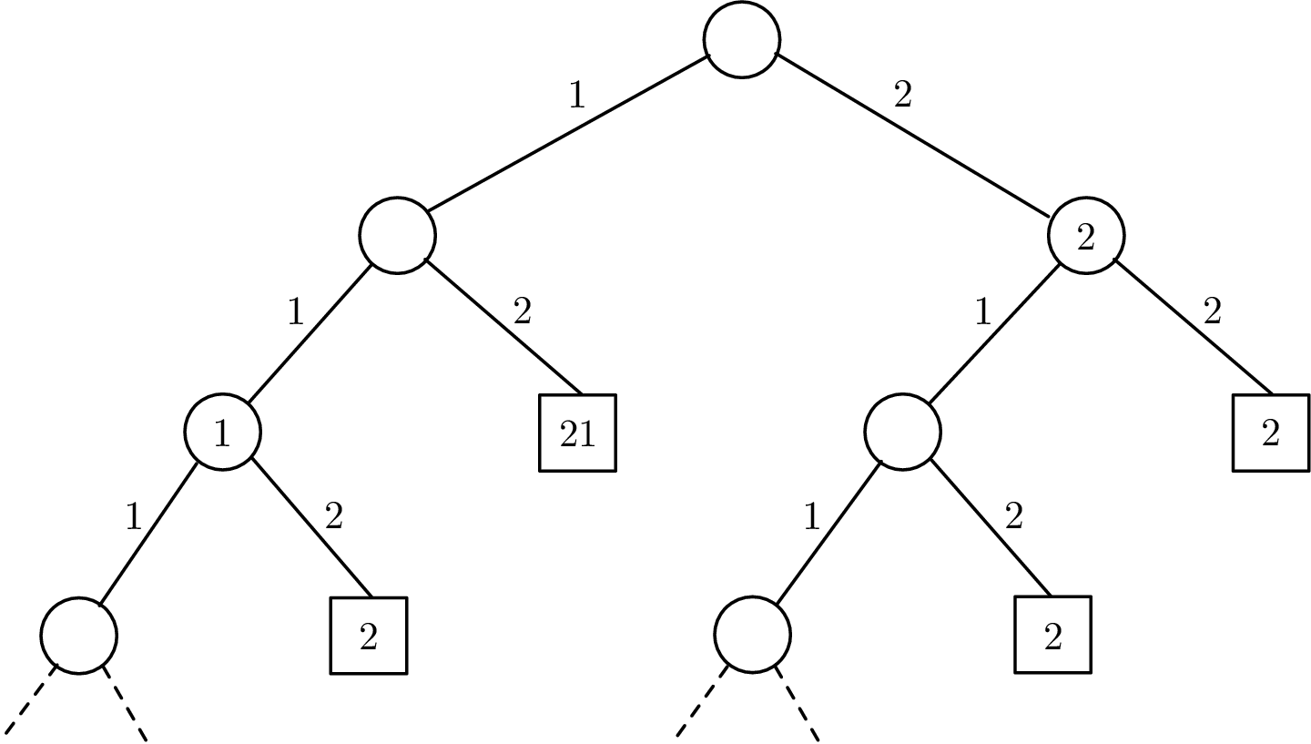
Let the coin process $\{X^{m}\}_{m=1}^{\infty}$ be the Markov chain induced by the transition matrix in Fig. 2 with the stationary initial distribution $P_{X_{1}}(1)=P_{X_{1}}(2)=1/2$ ; let $Y^{2}=(Y_{1},Y_{2})$ be $2$ symbols of i.i.d. random variables with $P_{Y_{j}}(1)=1/3$ and $P_{Y_{j}}(2)=2/3$ for $j=1,2$ . In this case, updates of the intervals are described in Fig. 3. Also, the algorithm tree is described in Fig. 4. For instance, when $X_{1}=2$ is observed, the algorithm outputs $Y_{1}=2$ ; then, if $(X_{2},X_{3})=(1,2)$ are observed after $X_{1}=2$ , the algorithm outputs $Y_{2}=2$ and terminates. On the other hand, when $(X_{1},X_{2})=(1,2)$ are observed, the algorithm first outputs $Y_{1}=2$ ; then, outputs $Y_{2}=1$ without further observing the coin process. In the latter case, the node in the algorithm tree is labeled by two symbols $(2,1)$ .

For notational convenience, we denote the function corresponding to the interval algorithm (cf. (4)) by $\phi_{\mathtt{int}}(\cdot)$ . Before verifying the validity of the algorithm (cf. (5)) carefully, we first examine the stopping time of the interval algorithm.

Theorem 4

For the interval algorithm, the overflow probability of the stopping time satisfies

\displaystyle\Pr(T>m)\leq P_{X^{m}}({\cal S}_{m}^{c}(\lambda))+P_{Y^{n}}({\cal T}_{n}^{c}(\tau))+2^{-\lambda+\tau+1},

where ${\cal S}_{m}(\lambda)$ and ${\cal T}_{n}(\tau)$ are defined as in (8) and (9), respectively.

Proof.

Let

\displaystyle{\cal D}_{m}:=\big\{x^{m}\in{\cal X}^{m}:\forall y^{n}\in{\cal Y}^{n},~{\cal I}_{x^{m}}\not\subseteq{\cal J}_{y^{n}}\big\}

and

\displaystyle{\cal E}_{m}:=\big\{x^{m}\in{\cal X}^{m}:\exists y^{n}\in{\cal T}_{n}(\tau)\mbox{ s.t. }{\cal I}_{x^{m}}\cap{\cal J}_{y^{n}}\neq\emptyset\big\}.

Then, since the algorithm does not terminate after observing $x^{m}$ if and only if $x^{m}\in{\cal D}_{m}$ , the overflow probability can be rewritten as

$\displaystyle\Pr(T>m)$	$\displaystyle=\sum_{x^{m}\in{\cal D}_{m}}P_{X^{m}}(x^{m})$
	$\displaystyle=\sum_{x^{m}\in{\cal D}_{m}\cap{\cal E}_{m}}P_{X^{m}}(x^{m})+\sum_{x^{m}\in{\cal D}_{m}\cap{\cal E}_{m}^{c}}P_{X^{m}}(x^{m})$
	$\displaystyle\leq\sum_{x^{m}\in{\cal D}_{m}\cap{\cal E}_{m}}P_{X^{m}}(x^{m})+P_{Y^{n}}({\cal T}_{n}^{c}(\tau)),$	(12)

where the inequality is justified as follows. Note that $x^{m}\in{\cal E}_{m}^{c}$ implies ${\cal I}_{x^{m}}\cap{\cal J}_{y^{n}}=\emptyset$ for every $y^{n}\in{\cal T}_{n}(\tau)$ , which further implies

\displaystyle\bigcup_{x^{m}\in{\cal E}_{m}^{c}}{\cal I}_{x^{m}}\subseteq\bigcup_{y^{n}\in{\cal T}^{c}_{n}(\tau)}{\cal J}_{y^{n}}.

Thus, by noting that $P_{X^{m}}(x^{m})=|{\cal I}_{x^{m}}|$ and $P_{Y^{n}}(y^{n})=|{\cal J}_{y^{n}}|$ , we have the inequality.

Furthermore, the first term of (12) can be bounded as

$\displaystyle\sum_{x^{m}\in{\cal D}_{m}\cap{\cal E}_{m}}P_{X^{m}}(x^{m})$	$\displaystyle=\sum_{x^{m}\in{\cal D}_{m}\cap{\cal E}_{m}\cap{\cal S}_{m}(\lambda)}P_{X^{m}}(x^{m})+\sum_{x^{m}\in{\cal D}_{m}\cap{\cal E}_{m}\cap{\cal S}_{m}^{c}(\lambda)}P_{X^{m}}(x^{m})$
	$\displaystyle\leq\sum_{x^{m}\in{\cal D}_{m}\cap{\cal E}_{m}\cap{\cal S}_{m}(\lambda)}P_{X^{m}}(x^{m})+P_{X^{m}}({\cal S}_{m}^{c}(\lambda))$
	$\displaystyle\leq\sum_{x^{m}\in{\cal D}_{m}\cap{\cal E}_{m}\cap{\cal S}_{m}(\lambda)}2^{-\lambda}+P_{X^{m}}({\cal S}_{m}^{c}(\lambda))$
	$\displaystyle\leq\|{\cal D}_{m}\cap{\cal E}_{m}\|2^{-\lambda}+P_{X^{m}}({\cal S}_{m}^{c}(\lambda))$
	$\displaystyle\leq 2\|{\cal T}_{n}(\tau)\|2^{-\lambda}+P_{X^{m}}({\cal S}_{m}^{c}(\lambda))$
	$\displaystyle\leq 2^{-\lambda+\tau+1}+P_{X^{m}}({\cal S}_{m}^{c}(\lambda)),$	(13)

where the second last inequality is justified as follows. By noting that $x^{m}\in{\cal D}_{m}\cap{\cal E}_{m}$ implies ${\cal I}_{x^{m}}\cap{\cal J}_{y^{n}}\neq\emptyset$ and ${\cal I}_{x^{m}}\not\subseteq{\cal J}_{y^{n}}$ for some $y^{n}\in{\cal T}_{n}(\tau)$ , we have

\displaystyle|{\cal D}_{m}\cap{\cal E}_{m}|\leq\sum_{y^{n}\in{\cal T}_{n}(\tau)}\sum_{x^{m}\in{\cal X}^{m}}\mathbf{1}\big[{\cal I}_{x^{m}}\cap{\cal J}_{y^{n}}\neq\emptyset,{\cal I}_{x^{m}}\not\subseteq{\cal J}_{y^{n}}\big].

For each fixed $y^{n}\in{\cal T}_{n}(\tau)$ , if there are more than two $x^{m}$ ’s satisfying ${\cal I}_{x^{m}}\cap{\cal J}_{y^{n}}\neq\emptyset$ , then all but the top and bottom ones must satisfy ${\cal I}_{x^{m}}\subseteq{\cal J}_{y^{n}}$ ; in other words, there are at most two $x^{m}$ ’s satisfying both the conditions in the indicator function. Thus, we have

\displaystyle\sum_{y^{n}\in{\cal T}_{n}(\tau)}\sum_{x^{m}\in{\cal X}^{m}}\mathbf{1}\big[{\cal I}_{x^{m}}\cap{\cal J}_{y^{n}}\neq\emptyset,{\cal I}_{x^{m}}\not\subseteq{\cal J}_{y^{n}}\big]\leq 2|{\cal T}_{n}(\tau)|.

Finally, by combining (12) and (13), we have the claimed bound. ∎

Now, we argue the validity of the interval algorithm. Clearly, if the coin process is deterministic, the random number generation is not possible. By using Theorem 4, we can prove that the interval algorithm exactly generate a target distribution as long as the coin process has “diverging randomness”.

Corollary 5

If the coin process $\bm{X}=\{X^{m}\}_{m=1}^{\infty}$ satisfies

\displaystyle\lim_{m\to\infty}P_{X^{m}}({\cal S}_{m}^{c}(\lambda))=0

(14)

for every $\lambda>0$ , where ${\cal S}_{m}(\lambda)$ is defined as in (8), then the interval algorithm is valid, i.e.,

\displaystyle\lim_{m\to\infty}\Pr(\phi_{\mathtt{int}}(X^{m})=y^{n})=P_{Y^{n}}(y^{n})

for every $y^{n}\in{\cal Y}^{n}$ .

Proof.

Upon observing $x^{m}\in{\cal X}^{m}$ , the interval algorithm terminates with output $y^{n}\in{\cal Y}^{n}$ if and only if ${\cal I}_{x^{m}}\subseteq{\cal J}_{y^{n}}$ . Thus, we have

\displaystyle\Pr(\phi_{\mathtt{int}}(X^{m})=y^{n})\leq P_{Y^{n}}(y^{n}).

(15)

Furthermore, since the lefthand side of (15) is non-decreasing in $m$ , it has a limit. To prove that the limit coincides with the righthand side, we apply Theorem 4 with

\displaystyle\tau=\max_{y^{n}\in\mathtt{supp}(P_{Y^{n}})}\log\frac{1}{P_{Y^{n}}(y^{n})},

where $\mathtt{supp}(P_{Y^{n}})$ is the support of distribution $P_{Y^{n}}$ . Then, we have

	$\displaystyle\Pr(\phi_{\mathtt{int}}(X^{m})\notin{\cal Y}^{n})$	$\displaystyle=\Pr(T>m)$
		$\displaystyle\leq P_{X^{m}}({\cal S}_{m}^{c}(\lambda))+2^{-\lambda+\tau+1}$

for any $\lambda$ . Since (14) holds for any $\lambda$ by assumption, by taking the limit $m\to\infty$ and $\lambda\to\infty$ with the diagonalization argument (cf. [9]), we have

\displaystyle\lim_{m\to\infty}\Pr(\phi_{\mathtt{int}}(X^{m})\in{\cal Y}^{n})=1,

which together with (15) implies the claim of the theorem.²² 2 Note that $a\leq A$ , $b\leq B$ , $A+B=1$ , and $a+b=1$ imply $1-b=a\leq A=1-B$ , i.e., $B\leq b$ . ∎

In fact, using Theorem 2, we can also prove that the same condition as Corollary 5 is necessary for exact random number generation by any algorithms.

Corollary 6

If the coin process $\bm{X}=\{X^{m}\}_{m=1}^{\infty}$ does not satisfy (14) for some $\lambda>0$ , then there exists a target distribution $P_{Y^{n}}$ with sufficiently large $n$ such that the validity (5) does not hold for any random number generation algorithms.

Proof.

Suppose that (14) does not hold for some $\lambda>0$ , i.e., there exists $\delta>0$ such that

\displaystyle P_{X^{m}}({\cal S}_{m}^{c}(\lambda))\geq\delta

for every sufficiently large $m$ . Let $\tau=\lambda-\log(\delta/2)$ . Then, by (7) of Theorem 2, we have

\displaystyle\Pr(T>m)\geq\frac{\delta}{2}-P_{Y^{n}}({\cal T}_{n}(\tau)).

This bound implies that, for any target distribution with min-entropy $H_{\min}(Y^{n})>\tau$ ,

\displaystyle\Pr(T>m)\geq\frac{\delta}{2}

for every sufficiently large $m$ . Thus, the validity (5) cannot be satisfied for some $y^{n}\in{\cal Y}^{n}$ . ∎

For instance, any absorbing Markov chain does not satisfy the sufficient condition of Corollary 5; note that absorbing Markov chains have $0$ spectral inf-entropy, i.e., $\underline{H}(\bm{X})=0$ . A further relaxed sufficient condition is that $\underline{H}(\bm{X})>0$ ; however, this relaxed condition is not necessary in general as the following example illustrates.

Example 7 (Harmonic Bernoulli Coin)

Let us consider independent but non-stationary Bernoulli trials $\bm{X}=\{X^{m}\}_{m=1}^{\infty}$ such that $P_{X_{i}}(1)=2^{-1/i}$ . Then, since the min-entropy (see the last paragraph of Section I for the definition) of $X^{m}$ is bounded from below as

	$\displaystyle H_{\min}(X^{m})$	$\displaystyle=\sum_{i=1}^{m}H_{\min}(X_{i})$
		$\displaystyle=\sum_{i=1}^{m}\frac{1}{i}$
		$\displaystyle\geq\ln(m+1),$

(14) is satisfied for any $\lambda>0$ . Thus, this coin process can be used for the interval algorithm. However, we can verify that $\underline{H}(\bm{X})=0$ as follows. Note that

	$\displaystyle\frac{1}{m}H(X^{m})$	$\displaystyle=\sum_{i=1}^{m}\frac{1}{m}H(X_{i})$
		$\displaystyle\leq h\bigg(\sum_{i=1}^{m}\frac{1}{m}P_{X_{i}}(1)\bigg)$

by concavity of the entropy. Furthermore, since $t\mapsto 2^{-t}$ is convex, we have

	$\displaystyle\sum_{i=1}^{m}\frac{1}{m}P_{X_{i}}(1)$	$\displaystyle=\sum_{i=1}^{m}\frac{1}{m}2^{-H_{\min}(X_{i})}$
		$\displaystyle\geq 2^{-\sum_{i=1}^{m}\frac{1}{m}H_{\min}(X_{i})}$
		$\displaystyle\geq 2^{-\frac{\ln m+1}{m}}$
		$\displaystyle\geq\frac{1}{2},$

which implies

\displaystyle\frac{1}{m}H(X^{m})\leq h\big(2^{-\frac{\ln m+1}{m}}\big).

Thus, by [9, Theorem 1.7.2], we have

\displaystyle\underline{H}(\bm{X})\leq\lim_{m\to\infty}\frac{1}{m}H(X^{m})=0.

On the other hand, if the probability distribution of each trial is $P_{X_{i}}(1)=2^{-1/i^{2}}$ , then, for any $\delta>0$ , we have

\displaystyle\lim_{m\to\infty}P_{X^{m}}({\cal S}_{m}^{c}(\pi^{2}/6+\delta))\geq\prod_{i=1}^{\infty}P_{X_{i}}(1)=2^{-\pi^{2}/6}.

Thus, this coin process cannot be used for any random number generation algorithms.

IV Asymptotic Analysis

IV-A General Results

In this section, we shall examine the asymptotic optimality of the interval algorithm. Recall the notations of information measures described in (1), (2), and (3). We start with the criterion of the overflow probability of the stopping time.

Definition 8

For a given random number generation algorithm converting $\bm{X}$ to $\bm{Y}$ , a rate $R\geq 0$ is defined to be achievable if the stopping time $T_{n}$ satisfies

\displaystyle\lim_{n\to\infty}\Pr(T_{n}>nR)=0.

Then, let $R^{\star}_{\mathtt{int}}(\bm{X},\bm{Y})$ and $R^{\star}(\bm{X},\bm{Y})$ be the infimum rates that are achievable by the interval algorithm and by any algorithm (not necessarily the interval algorithm), respectively.

Theorem 9

For given coin process $\bm{X}$ with $\underline{H}(\bm{X})>0$ and target process $\bm{Y}$ , the infimum achievable rate of the interval algorithm satisfies

\displaystyle R^{\star}_{\mathtt{int}}(\bm{X},\bm{Y})\leq\frac{\overline{H}(\bm{Y})}{\underline{H}(\bm{X})}.

(16)

On the other hand, the infimum achievable rate of any algorithm satisfies

\displaystyle R^{\star}(\bm{X},\bm{Y})\geq\max\bigg[\frac{\overline{H}(\bm{Y})}{\overline{H}(\bm{X})},\frac{\underline{H}(\bm{Y})}{\underline{H}(\bm{X})}\bigg].

(17)

Proof.

We first prove (16). Fix arbitrary $\delta_{1},\delta_{2}>0$ . By applying Theorem 4 with

	$\displaystyle m_{n}$	$\displaystyle=n\bigg(\frac{\overline{H}(\bm{Y})}{\underline{H}(\bm{X})}+\delta_{2}\bigg),$
	$\displaystyle R$	$\displaystyle=\frac{\overline{H}(\bm{Y})}{\underline{H}(\bm{X})}+\delta_{2},$
	$\displaystyle\lambda$	$\displaystyle=m_{n}(\underline{H}(\bm{X})-\delta_{1}),$
	$\displaystyle\tau$	$\displaystyle=n(\overline{H}(\bm{Y})+\delta_{1}),$

we can bound the overflow probability of the stopping time for the interval algorithm as

	$\displaystyle\Pr(T_{n}>nR)$	$\displaystyle\leq\Pr\bigg(\frac{1}{m_{n}}\log\frac{1}{P_{X^{m_{n}}}(X^{m_{n}})}<\underline{H}(\bm{X})-\delta_{1}\bigg)+\Pr\bigg(\frac{1}{n}\log\frac{1}{P_{Y^{n}}(Y^{n})}>\overline{H}(\bm{Y})+\delta_{1}\bigg)$
		$\displaystyle~~~+\exp\bigg[-n\bigg\{\delta_{2}(\underline{H}(\bm{X})-\delta_{1})-\delta_{1}\bigg(\frac{\overline{H}(\bm{Y})}{\underline{H}(\bm{X})}+1\bigg)\bigg\}+1\bigg].$

Thus, if we take $\delta_{1}$ sufficiently small compared to $\delta_{2}$ , we have

\displaystyle\lim_{n\to\infty}\Pr(T_{n}>nR)=0,

which implies that $R=\overline{H}(\bm{Y})/\underline{H}(\bm{X})+\delta_{2}$ is achievable. Since $\delta_{2}>0$ is arbitrary, we have (16).

Next, we prove the first bound of (17). Fix arbitrary $\delta_{1},\delta_{2}>0$ . By applying (6) of Theorem 2 with

	$\displaystyle m_{n}$	$\displaystyle=n\bigg(\frac{\overline{H}(\bm{Y})}{\overline{H}(\bm{X})}-\delta_{2}\bigg),$
	$\displaystyle R$	$\displaystyle=\frac{\overline{H}(\bm{Y})}{\overline{H}(\bm{X})}-\delta_{2},$
	$\displaystyle\lambda$	$\displaystyle=m_{n}(\overline{H}(\bm{X})+\delta_{1}),$
	$\displaystyle\tau$	$\displaystyle=n(\overline{H}(\bm{Y})-\delta_{1}),$

for any random number generation algorithms, we have

	$\displaystyle\Pr(T_{n}>nR)$	$\displaystyle\geq\Pr\bigg(\frac{1}{n}\log\frac{1}{P_{Y^{n}}(Y^{n})}>\overline{H}(\bm{Y})-\delta_{1}\bigg)-\Pr\bigg(\frac{1}{m_{n}}\log\frac{1}{P_{X^{m_{n}}}(X^{m_{n}})}\geq\overline{H}(\bm{X})+\delta_{1}\bigg)$
		$\displaystyle~~~-\exp\bigg[-n\bigg\{\delta_{2}(\overline{H}(\bm{X})+\delta_{1})-\delta_{1}\bigg(\frac{\overline{H}(\bm{Y})}{\overline{H}(\bm{X})}+1\bigg)\bigg\}\bigg].$

Thus, if we take $\delta_{1}$ sufficiently small compared to $\delta_{2}$ , the definition of $\overline{H}(\bm{Y})$ leads to

\displaystyle\liminf_{n\to\infty}\Pr(T_{n}>nR)>0,

which implies that $R=\overline{H}(\bm{Y})/\overline{H}(\bm{X})-\delta_{2}$ is not achievable. Since $\delta_{2}$ is arbitrary, we have the first bound of (17). We can prove the second bound of (17) in a similar manner by using (7) of Theorem 2. ∎

When either the coin or the target process has one point spectrum, we immediately obtain the following corollary from Theorem 9.

Corollary 10

When the spectral sup-entropy $\overline{H}(\bm{X})$ and inf-entropy $\underline{H}(\bm{X})$ of coin process coincide with its entropy rate $H(\bm{X})$ ,³³ 3 When $\overline{H}(\bm{X})=\underline{H}(\bm{X})$ , called the one-point spectrum, the limit in (3) exists, and we have $\overline{H}(\bm{X})=\underline{H}(\bm{X})=H(\bm{X})$ (cf. [9, Theorem 1.7.2]). we have

\displaystyle R^{\star}_{\mathtt{int}}(\bm{X},\bm{Y})=R^{\star}(\bm{X},\bm{Y})=\frac{\overline{H}(\bm{Y})}{H(\bm{X})}.

On the other hand, when spectral sup-entropy $\overline{H}(\bm{Y})$ and inf-entropy $\underline{H}(\bm{Y})$ of the target process coincide with its entropy rate $H(\bm{Y})$ , we have

\displaystyle R^{\star}_{\mathtt{int}}(\bm{X},\bm{Y})=R^{\star}(\bm{X},\bm{Y})=\frac{H(\bm{Y})}{\underline{H}(\bm{X})}.

Next, we investigate the average stopping time $\mathbb{E}[T_{n}]$ .

Definition 11

For a given random number generation algorithm converting $\bm{X}$ to $\bm{Y}$ , a rate $L\geq 0$ is defined to be average achievable if the average stopping time $\mathbb{E}[T_{n}]$ satisfies

\displaystyle\limsup_{n\to\infty}\frac{\mathbb{E}[T_{n}]}{n}\leq L.

Then, let $L_{\mathtt{int}}^{\star}(\bm{X},\bm{Y})$ and $L^{\star}(\bm{X},\bm{Y})$ be the infimum rates that are average achievable by the interval algorithm and by any algorithm (not necessarily the interval algorithm), respectively.

In the following argument, as a technical condition, we assume that the upper and lower tails of the information spectrum of the coin process vanish sufficiently rapidly in the following sense: for any $\delta>0$ , there exist constants $K$ and $m_{0}=m_{0}(\delta,K)$ such that

\displaystyle\Pr\bigg(\frac{1}{m}\log\frac{1}{P_{X^{m}}(X^{m})}\geq\overline{H}(\bm{X})+\delta\bigg)\leq\frac{K}{m^{2}}

(18)

and

\displaystyle\Pr\bigg(\frac{1}{m}\log\frac{1}{P_{X^{m}}(X^{m})}\leq\underline{H}(\bm{X})-\delta\bigg)\leq\frac{K}{m^{2}}

(19)

for every $m\geq m_{0}$ . In fact, i.i.d. processes, irreducible Markov processes, or mixture of those processes satisfy much stronger requirement, i.e., the upper and lower tails vanish exponentially [6].

Now, we are ready to present the asymptotic behavior of the average stopping time.

Theorem 12

For given coin process $\bm{X}$ satisfying (19) and target process $\bm{Y}$ , the infimum average achievable rate of the interval algorithm satisfies

\displaystyle L_{\mathtt{int}}^{\star}(\bm{X},\bm{Y})\leq\frac{H(\bm{Y})}{\underline{H}(\bm{X})}.

(20)

On the other hand, for given coin process $\bm{X}$ satisfying (18) and target process $\bm{Y}$ , the infimum average achievable rate of any algorithm satisfies

\displaystyle L^{\star}(\bm{X},\bm{Y})\geq\frac{H(\bm{Y})}{\overline{H}(\bm{X})}.

(21)

Proof.

We first prove (20). By using the identity on the expectation (eg. see [3, Eq. (21.9)]), we can write

\displaystyle\mathbb{E}[T_{n}]=\int_{0}^{\infty}\Pr(T_{n}>z)dz.

(22)

Fix arbitrary $\delta>0$ . For each $z$ , by applying Theorem 4 with $\lambda=\lfloor z\rfloor(\underline{H}(\bm{X})-\delta)$ and $\tau=z(\underline{H}(\bm{X})-2\delta)$ , we have

	$\displaystyle\Pr(T_{n}>z)$	$\displaystyle\leq\Pr(T_{n}>\lfloor z\rfloor)$
		$\displaystyle\leq\Pr\bigg(\frac{1}{\lfloor z\rfloor}\log\frac{1}{P_{X^{\lfloor z\rfloor}}(X^{\lfloor z\rfloor})}<\underline{H}(\bm{X})-\delta\bigg)+\Pr\bigg(\frac{1}{(\underline{H}(\bm{X})-2\delta)}\log\frac{1}{P_{Y^{n}}(Y^{n})}>z\bigg)+2^{-\delta z+1}.$

The integral of the first term is bounded as

	$\displaystyle\int_{0}^{\infty}\Pr\bigg(\frac{1}{\lfloor z\rfloor}\log\frac{1}{P_{X^{\lfloor z\rfloor}}(X^{\lfloor z\rfloor})}<\underline{H}(\bm{X})-\delta\bigg)dz$	$\displaystyle\leq m_{0}+\int_{m_{0}}^{\infty}\frac{K}{(z-1)^{2}}dz$
		$\displaystyle=m_{0}+\frac{K}{(m_{0}-1)},$

where the inequality follows from (19); the integral of the second term is

\displaystyle\int_{0}^{\infty}\Pr\bigg(\frac{1}{(\underline{H}(\bm{X})-2\delta)}\log\frac{1}{P_{Y^{n}}(Y^{n})}>z\bigg)dz=\frac{H(Y^{n})}{(\underline{H}(\bm{X})-2\delta)},

where we used the identity on the expectation again; the integral of the third term is given by $\frac{2}{\delta\ln 2}$ . By substituting these evaluations into (22), we obtain

\displaystyle\limsup_{n\to\infty}\frac{\mathbb{E}[T_{n}]}{n}\leq\frac{H(\bm{Y})}{(\underline{H}(\bm{X})-2\delta)}.

Since $\delta>0$ is arbitrary, we have (20).

Next, we prove (21). We start with (22). Fix arbitrary $\delta>0$ . For each $z$ , by applying (6) of Theorem 2 with $\lambda=\lceil z\rceil(\overline{H}(\bm{X})+\delta)$ and $\tau=z(\overline{H}(\bm{X})+2\delta)$ , we have

	$\displaystyle\Pr(T_{n}>z)$
		$\displaystyle\geq\Pr(T_{n}>\lceil z\rceil)$
		$\displaystyle\geq\Pr\bigg(\frac{1}{(\overline{H}(\bm{X})+2\delta)}\log\frac{1}{P_{Y^{n}}(Y^{n})}>z\bigg)-\Pr\bigg(\frac{1}{\lceil z\rceil}\log\frac{1}{P_{X^{\lceil z\rceil}}(X^{\lceil z\rceil})}\geq\overline{H}(\bm{X})+\delta\bigg)-2^{-\delta(z-1)+\overline{H}(\bm{X})}.$

By evaluating the integral of each term in a similar manner as above and by substituting them into (22), we obtain

\displaystyle\limsup_{n\to\infty}\frac{\mathbb{E}[T_{n}]}{n}\geq\frac{H(\bm{Y})}{(\overline{H}(\bm{X})+2\delta)}.

Since $\delta>0$ is arbitrary, we have (21). ∎

When the coin process has one point spectrum, we immediately obtain the following corollary from Theorem 12.

Corollary 13

When the coin process satisfies (18), (19), and $\overline{H}(\bm{X})$ and $\underline{H}(\bm{X})$ coincide with $H(\bm{X})$ , we have

\displaystyle L_{\mathtt{int}}^{\star}(\bm{X},\bm{Y})=L^{\star}(\bm{X},\bm{Y})=\frac{H(\bm{Y})}{H(\bm{X})}.

It should be noted that the target process $\bm{Y}$ need not to have one point spectrum in Corollary 13.

Remark 14

When both the coin and target processes are ergodic, it was shown in [31] that the normalized stopping time of the interval algorithm almost surely converges to the ratio of the entropy rates, i.e.,

\displaystyle\lim_{n\to\infty}\frac{T_{n}}{n}=\frac{H(\bm{Y})}{H(\bm{X})}~~~\mbox{a.s.}

(23)

This result immediately implies

\displaystyle R_{\mathtt{int}}^{\star}(\bm{X},\bm{Y})=\frac{H(\bm{Y})}{H(\bm{X})}.

However, in order to derive

\displaystyle L_{\mathtt{int}}^{\star}(\bm{X},\bm{Y})=\frac{H(\bm{Y})}{H(\bm{X})}

from (23), we need to prove uniform integrability of $T_{n}/n$ (cf. [3, Theorem 16.14]), which is a cumbersome problem thought it may be possible.

In the next subsections, we shall illustrate the general results above with concrete classes of coin/target processes.

IV-B Markov Coin/Target Processes

As a coin process, we consider a Markov chain $\bm{X}=\{X^{m}\}_{m=1}^{\infty}$ on ${\cal X}$ induced by a transition matrix $W(x|x^{\prime})$ . Suppose that $W$ is irreducible, i.e., for any $x,x^{\prime}\in{\cal X}$ , there exists an integer $k\geq 1$ such that $W^{k}(x|x^{\prime})>0$ . When $W$ is irreducible, there exists a unique stationary distribution $\pi$ [19]. For the stationary distribution, let

\displaystyle H^{W}(X):=\sum_{x,x^{\prime}}\pi(x^{\prime})W(x|x^{\prime})\log\frac{1}{W(x|x^{\prime})},

which coincides with the entropy rate of the Markov chain when the initial distribution is $\pi$ [5].

We use the following bounds from the large deviation theory (cf. [6, 36]).

Lemma 15

Let $\bm{X}=\{X^{m}\}_{m=1}^{\infty}$ be a Markov chain induced by an irreducible transition matrix $W$ with arbitrary initial distribution $P_{X_{1}}$ . For $\delta>0$ , there exist $\overline{E}(\delta),\underline{E}(\delta)>0$ such that

	$\displaystyle\Pr\bigg(\frac{1}{m}\sum_{i=2}^{m}\log\frac{1}{W(X_{i}\|X_{i-1})}\geq H^{W}(X)+\delta\bigg)$	$\displaystyle\leq 2^{-m\overline{E}(\delta)},$
	$\displaystyle\Pr\bigg(\frac{1}{m}\sum_{i=2}^{m}\log\frac{1}{W(X_{i}\|X_{i-1})}\leq H^{W}(X)-\delta\bigg)$	$\displaystyle\leq 2^{-m\underline{E}(\delta)}$

for every sufficiently large $m$ .

From Lemma 15 and [9, Theorem 1.7.2], for any initial distribution $P_{X_{1}}$ , we have

\displaystyle\underline{H}(\bm{X})=H(\bm{X})=\overline{H}(\bm{X})=H^{W}(X).

(24)

Furthermore, the conditions in (18) and (19) are also satisfied.

For the target process, we consider a Markov chain $\bm{Y}=\{Y^{n}\}_{n=1}^{\infty}$ on ${\cal Y}$ induced by a transition matrix $V$ . Suppose that $V$ is not irreducible but there is no transient class (cf. [19]), i.e., the transition matrix can be decomposed as a direct sum form:

\displaystyle V=\bigoplus_{\xi=1}^{r}V_{\xi},

where $V_{\xi}$ is the irreducible transition matrix on irreducible class ${\cal Y}_{\xi}\subset{\cal Y}$ for $\xi=1,\ldots,r$ . When the initial state is $Y_{1}\in{\cal Y}_{\xi}$ , then $Y_{2},Y_{3},\ldots$ remain in the same irreducible class ${\cal Y}_{\xi}$ . Thus, for the weight

\displaystyle w(\xi)=\Pr\big(Y_{1}\in{\cal Y}_{\xi}\big)

of each irreducible class induced from the initial distribution $P_{Y_{1}}$ , the Markov chain $Y^{n}$ can be regarded as a mixture of irreducible Markov chains, i.e.,

\displaystyle\Pr\big(Y^{n}=y^{n}\big)=\sum_{\xi=1}^{r}w(\xi)\Pr\big(Y^{n}=y^{n}|Y_{1}\in{\cal Y}_{\xi}\big).

Let $\pi_{\xi}$ be the stationary distribution of $V_{\xi}$ , and let

\displaystyle H^{V_{\xi}}(Y):=\sum_{y,y^{\prime}\in{\cal Y}_{\xi}}\pi_{\xi}(y^{\prime})V_{\xi}(y|y^{\prime})\log\frac{1}{V_{\xi}(y|y^{\prime})}

be the entropy rate of $\xi$ -th irreducible class. Then, by the argument in [9, Sec. 1.4], the information spectral quantities and the entropy rate are given as follows (see also Fig. 5):⁴⁴ 4 When transition matrix $V$ has transient class, the information spectral quantities and the entropy rate are given by the same formulae; however, weight $w(\xi)$ is determined as the limiting probability such that the initial state is eventually absorbed into irreducible class ${\cal Y}_{\xi}$ (cf. [19, Chapter 8]).

	$\displaystyle\overline{H}(\bm{Y})$	$\displaystyle=\max\big\{H^{V_{\xi}}(Y):1\leq\xi\leq r,w(\xi)>0\big\},$
	$\displaystyle\underline{H}(\bm{Y})$	$\displaystyle=\min\big\{H^{V_{\xi}}(Y):1\leq\xi\leq r,w(\xi)>0\big\},$
	$\displaystyle H(\bm{Y})$	$\displaystyle=\sum_{\xi=1}^{r}w(\xi)H^{V_{\xi}}(Y).$

From the above arguments along with Corollary 10 and Corollary 13, we have

\displaystyle R_{\mathtt{int}}^{\star}(\bm{X},\bm{Y})=R^{\star}(\bm{X},\bm{Y})=\frac{1}{H^{W}(X)}\max\big\{H^{V_{\xi}}(Y):1\leq\xi\leq r,w(\xi)>0\big\}

and

\displaystyle L_{\mathtt{int}}^{\star}(\bm{X},\bm{Y})=L^{\star}(\bm{X},\bm{Y})=\frac{1}{H^{W}(X)}\sum_{\xi=1}^{r}w(\xi)H^{V_{\xi}}(Y).

IV-C Target Process with Continuous Spectrum

As a coin process, we again consider a Markov chain $\bm{X}=\{X^{m}\}_{m=1}^{\infty}$ on ${\cal X}$ induced by an irreducible transition matrix $W$ . As we have seen in Section IV-B, the spectral sup-entropy and inf-entropy coincide with the entropy rate, and they are given by $H^{W}(X)$ .

Let $\{V_{\xi}\}_{\xi\in\Xi}$ be a parametrized family of irreducible matrix on ${\cal Y}$ , and let

\displaystyle P_{Y^{n}}(y^{n})=\int P_{Y_{\xi}}^{n}(y^{n})dw(\xi)

be the mixture of Markov process with arbitrary weight $w(\xi)$ , where

\displaystyle P_{Y_{\xi}^{n}}(y^{n})=P_{Y_{\xi,1}}(y_{1})\prod_{i=2}^{n}V_{\xi}(y_{i}|y_{i-1}).

Then, for the target process $\bm{Y}=\{Y^{n}\}_{n=1}^{\infty}$ , we have⁵⁵ 5 For a measurable function $Z_{\xi}$ of $\xi$ , the essential supremum with respect to $w(\xi)$ is defined as $w\mbox{-ess.~sup }Z_{\xi}:=\inf\{\alpha:\Pr\{Z_{\xi}>\alpha\}=0$ . (cf. [9, Theorem 1.4.3])

\displaystyle\overline{H}(\bm{Y})=w\mbox{-ess.~sup }H^{V_{\xi}}(Y)

and (cf. [9, Remark 1.7.3])

\displaystyle H(\bm{Y})=\int H^{V_{\xi}}(Y)dw(\xi).

For the above described coin process and target process, Corollary 10 and Corollary 13 immediately provide

\displaystyle R^{\star}_{\mathtt{int}}(\bm{X},\bm{Y})=R^{\star}(\bm{X},\bm{Y})=\frac{1}{H^{W}(X)}w\mbox{-ess.~sup }H^{V_{\xi}}(Y)

and

\displaystyle L^{\star}_{\mathtt{int}}(\bm{X},\bm{Y})=L^{\star}(\bm{X},\bm{Y})=\frac{1}{H^{W}(X)}\int H^{V_{\xi}}(Y)dw(\xi).

V Connection to Fixed-Length Random Number Generation

In this section, we shall point out a connection between the problem of fixed-length random number generation (FL-RNG), and the variable-length random number generation (VL-RNG).⁶⁶ 6 Here, we fix the length of target random variables, and consider RNG algorithms with fixed/variable length of coin random variables. As in the previous sections, let $\bm{X}=\{X^{m}\}_{m=1}^{\infty}$ and $\bm{Y}=\{Y^{n}\}_{n=1}^{\infty}$ be the coin and target processes. An FL-RNG algorithm is described by a deterministic function $\psi:{\cal X}^{m}\to{\cal Y}^{n}$ , and the approximation error is defined by

\displaystyle\Delta_{m}:=\|P_{\tilde{Y}^{n}}-P_{Y^{n}}\|_{1}

for $\tilde{Y}^{n}=\psi(X^{m})$ , where $\|P-Q\|_{1}:=\frac{1}{2}\sum_{x}|P(x)-Q(x)|$ is the variational distance between two distributions $P$ and $Q$ .

In the problem of source coding, it is recognized that there is an intimate connection between the error probability of almost lossless fixed-length (FL) code and the overflow probability of the code length of variable-length (VL) code (eg. see [18, 30, 16]). More specifically, for a given VL code, we can construct a FL code such that the error probability is the same as the overflow probability of the original VL code; and vice versa. In a similar vein, we can convert a given VL-RNG algorithm to an FL-RNG algorithm as follows.

Proposition 16

For a given VL-RNG algorithm $\phi$ satisfying (5), there exists an FL-RNG algorithm $\psi$ such that the approximation error satisfies

\displaystyle\Delta_{m}\leq\Pr\big(T>m\big),

where $T$ is the stopping time of $\phi$ .

Proof.

For the set ${\cal L}_{\phi}$ of all leaves, let ${\cal B}=\{s\in{\cal L}_{\phi}:|s|\leq m\}$ . Recall that, by our convention, we denote $\phi(x^{m})=y^{n}$ if the algorithm terminates with output $\phi(x^{i})=y^{n}$ for some $i\leq m$ , and $\phi(x^{m})=\bot$ otherwise. By using these notations, we set

\displaystyle\psi(x^{m})=\left\{\begin{array}[]{ll}\phi(x^{m})&\mbox{if }\phi(x^{m})\in{\cal Y}^{n}\\ b^{n}&\mbox{else}\end{array}\right.

where $b^{n}\in{\cal Y}^{n}$ is an arbitrarily fixed sequence. Then, since

	$\displaystyle P_{\tilde{Y}^{n}}(b^{n})$	$\displaystyle=\sum_{s\in{\cal B}:\atop\phi(s)=b^{n}}P_{X^{\|s\|}}(s)+\sum_{s\in{\cal L}_{\phi}\backslash{\cal B}}P_{X^{\|s\|}}(s)$
		$\displaystyle\geq\sum_{s\in{\cal L}_{\phi}:\atop\phi(s)=b^{n}}P_{X^{\|s\|}}(s)$
		$\displaystyle=P_{Y^{n}}(b^{n})$

and

	$\displaystyle P_{\tilde{Y}^{n}}(y^{n})$	$\displaystyle=\sum_{s\in{\cal B}:\atop\phi(s)=y^{n}}P_{X^{\|s\|}}(s)$
		$\displaystyle\leq\sum_{s\in{\cal L}_{\phi}:\atop\phi(s)=y^{n}}P_{X^{\|s\|}}(s)$
		$\displaystyle=P_{Y^{n}}(y^{n})$

for every $y^{n}\neq b^{n}$ , we have

	$\displaystyle\Delta_{m}$	$\displaystyle=P_{\tilde{Y}^{n}}(b^{n})-P_{Y^{n}}(b^{n})$
		$\displaystyle=\sum_{s\in{\cal L}_{\phi}\backslash{\cal B}:\atop\phi(s)\neq b^{n}}P_{X^{\|s\|}}(s)$
		$\displaystyle\leq\sum_{s\in{\cal L}_{\phi}\backslash{\cal B}}P_{X^{\|s\|}}(s)$
		$\displaystyle=\Pr\big(T>m\big),$

where the first equality follows from an alternative expression of the variational distance (eg. see [5, Eq. (11.137)]). ∎

As we can find from the proof of Proposition 16, we can convert any VL-RNG algorithm to a FL-RNG algorithm just by stopping the VL-RNG algorithm after a prescribed number of coin tosses. In fact, the achievability bound for the FL-RNG [9, Lemma 2.1.1] can be also attained by the modified version of the interval algorithm via Proposition 16 and Theorem 4 up to a negligible constant factor; in the asymptotic regime, if we set $m=nR$ with $R>\overline{H}(\bm{Y})/\underline{H}(\bm{X})$ , then Theorem 9 guarantees that the approximation error $\Delta_{m}$ of the FL-RNG converges to $0$ (cf. Theorem [9, Theorem 2.1.1]). Conversely, even though we proved the converse bound for the VL-RNG (Theorem 2) directly in Section II, we can provide an alternative proof by combining Proposition 16 and the converse bound for the FL-RNG in [9, Lemma 2.1.2]; in the asymptotic regime, the converse bound in Theorem 9, i.e., $R\geq\max[\overline{H}(\bm{Y})/\overline{H}(\bm{X}),\underline{H}(\bm{Y})/\underline{H}(\bm{X})]$ for every achievable rate $R$ , can be obtained from Proposition 16 and [9, Theorem 2.1.2]. Unlike the source coding, the opposite claim, i.e., possibility of converting a FL-RNG to a VL-RNG, is not clear in general.

VI Discussion

In this paper, we revisited the problem of exactly generating a random process with another random process, and proved the optimality of the interval algorithm when either the coin or the target process has one point spectrum. However, when both the coin and the target processes have spreading spectrum, the achievability and the converse bounds derived in this paper do not coincide. At least, there is room for improvement on the achievability bound; for instance, when the coin process and the target process are identical and have spreading spectrum, the interval algorithm apparently attains the unit rate but the upper bounds in Theorem 9 and Theorem 12 are loose. In order to derive tighter bounds, instead of the upper and lower limits of the spectrums, we need to analyze spreading spectrums more carefully. For the random number generation with approximation error, such a direction of research was conducted in [21, 2].

In a similar vein, the bounds derived in this paper may not be tight for finite block length regime in general. When either the coin process or the target process is unbiased and the other process is i.i.d., by an application of the central limit theorem to the bounds in Theorem 2 and Theorem 4, we can derive bounds that coincide up to the so-called second-order rate [13, 26]. In other words, the interval algorithm is optimal up to the second-order rate in that case. It is an important research direction to conduct the finite block length analysis of the interval algorithm when both the coin and target processes are biased. It should be noted that, when the coin process is i.i.d., the average stopping time of the interval algorithm is known to be tight up to ${\cal O}(1)$ term [10].

Another important research direction is the interval algorithm with finite precision arithmetic. In order to implement the interval algorithm, the updates of intervals must be conducted with finite precision arithmetic in practice. Such a direction of research was conducted in [33] for i.i.d. processes.

References

[1] J. Abrahams, “Generation of discrete distributions from biased coins,” IEEE Trans. Inform. Theory, vol. 42, no. 5, pp. 1541–1546, September 1996.
[2] Y. Altuğ and A. B. Wagner, “Source and channel simulation using arbitrary randomness,” IEEE Trans. Inform. Theory, vol. 58, no. 3, pp. 1345–1360, March 2012.
[3] P. Billingsley, Probability and Measure. JOHN WILEY & SONS, 1995.
[4] M. Blum, “Independent unbiased coin flip from a correlated biased source — a finite state markov chain,” Combinatorica, vol. 6, no. 2, pp. 97–108, 1986.
[5] T. M. Cover and J. A. Thomas, Elements of Information Theory, 2nd ed. John Wiley & Sons, 2006.
[6] A. Dembo and O. Zeitouni, Large Deviations Techniques and Applications, 2nd ed. Springer, 1998.
[7] P. Elias, “The efficient construction of an unbiased random sequence,” The Annals of Mathematical Statistics, vol. 43, no. 3, pp. 865–870, 1972.
[8] T. S. Han, “Theorems on the variable-length intrinsic randomness,” IEEE Trans. Inform. Theory, vol. 46, no. 6, pp. 2108–2116, September 2000.
[9] ——, Information-Spectrum Methods in Information Theory. Springer, 2003.
[10] T. S. Han and M. Hoshi, “Interval algorithm for random number generation,” IEEE Trans. Inform. Theory, vol. 43, no. 2, pp. 599–611, March 1997.
[11] T. S. Han and S. Verdú, “Approximation theory of output statistics,” IEEE Trans. Inform. Theory, vol. 39, no. 3, pp. 752–772, May 1993.
[12] M. Hayashi, “Second-order asymptotics in fixed-length source coding and intrinsic randomness,” IEEE Trans. Inform. Theory, vol. 54, no. 10, pp. 4619–4637, October 2008.
[13] ——, “Information spectrum approach to second-order coding rate in channel coding,” IEEE Trans. Inform. Theory, vol. 55, no. 11, pp. 4947–4966, November 2009.
[14] W. Hoeffding and G. Simons, “Unbiased coin tossing with a biased coin,” The Annals of Mathematical Statistics, vol. 41, no. 2, pp. 341–352, 1970.
[15] D. Knuth and A. Yao, “The complexity of nonuniform random number generation,” Algorithms and Complexity, New Directions and Results, pp. 357–428, 1976.
[16] I. Kontoyiannis and S. Verdú, “Optimal lossless data compression: Non-asymptotic and asymptotics,” IEEE Trans. Inform. Theory, vol. 60, no. 2, pp. 777–795, February 2014.
[17] W. Kumagai and M. Hayashi, “Second-order asymptotics of conversions of distributions and entangled states based on Rayleigh-Normal probability distributions,” IEEE Trans. Inform. Theory, vol. 63, no. 3, pp. 1829–1857, March 2017.
[18] N. Merhav and D. L. Neuhoff, “Variable-to-fixed length codes provides better large deviation performance than fixed-to-variable length codes,” IEEE Trans. Inform. Theory, vol. 38, no. 1, pp. 135–140, January 1992.
[19] C. D. Meyer, Matrix Analysis and Applied Linear Algebra. SIAM: Society for Industrial and Applied Mathematics, 2010.
[20] J. Muramatsu and F. Kanaya, “Almost-sure variable-length source coding theorem for general sources,” IEEE Trans. Inform. Theory, vol. 45, no. 1, pp. 337–342, January 1999.
[21] H. Nagaoka and S. Miyake, “Approximation of stochastic processes and information spectra,” in Proceedings of 19th Symposium on Information Theory and Its Applications (SITA ’96), 1996, pp. 117–120.
[22] R. Nomura and T. S. Han, “Second-order resolvability, intrinsic randomness, and fixed-length source coding for mixed sources: Information spectrum approach,” IEEE Trans. Inform. Theory, vol. 59, no. 1, pp. 1–16, January 2013.
[23] Y. Oohama, “Performance analysis of the interval algorithm for random number generation based on number systems,” IEEE Trans. Inform. Theory, vol. 57, no. 3, pp. 1177–1185, March 2011.
[24] ——, “Performance analysis of the interval algorithm for random number generation in the case of Markov coin tossing,” in Proceedings of 2016 International Symposium on Nonlinear Theory and Its Applications, Yugawara, Japan, November 2016, pp. 245–248.
[25] Y. Peres, “Iterating von Neumann’s procedure for extracting random bits,” The Annals of Statistics, vol. 20, no. 1, pp. 590–597, 1992.
[26] Y. Polyanskiy, H. V. Poor, and S. Verdu, “Channel coding rate in the finite blocklength regime,” IEEE Trans. Inform. Theory, vol. 56, no. 5, pp. 2307–2359, May 2010.
[27] J. R. Roche, “Efficient generation of random variables from biased coins,” in IEEE International Symposium on Information Theory, 1991, p. 169.
[28] P. Samuelson, “Constructing an unbiased random sequence,” Journal of the American Statistical Association, vol. 63, pp. 1526–1527, 1968.
[29] P. C. Shields, The Ergodic Theory of Discrete Sample Paths. American Mathematical Society, 1996.
[30] O. Uchida and T. S. Han, “The optimal overflow and underflow probabilities of variable-length coding for the general sources,” IEICE Trans. Fundamentals, vol. E84-A, no. 10, pp. 2457–2465, October 2001.
[31] T. Uyematsu and F. Kanaya, “Almost sure convergence theorems of rate of coin tosses for random number generation by interval algorithm,” in Proceedings of 22nd Symposium on Information Theory and Its Applications (SITA ’99), 1999, pp. 213–216.
[32] ——, “Channel simulation by interval algorithm: A performance analysis of interval algorithm,” IEEE Trans. Inform. Theory, vol. 45, no. 6, pp. 2121–2129, September 1999.
[33] T. Uyematsu and Y. Li, “Two algorithms for random number generation implemented by using arithmetic of limited precision,” IEICE Trans. Fundamentals, vol. E86A, no. 10, pp. 2542–2551, October 2003.
[34] S. Vembu and S. Verdu, “Generating random bits from arbitrary source:fundamental limits,” IEEE Trans. Inform. Theory, vol. 41, no. 5, pp. 1322–1332, September 1995.
[35] J. von Neumann, “Various techniques used in connection with random digits,” Notes by G. E. Forsythe, National Bureau of Standards, Applied Math Series, vol. 12, pp. 36–38, 1951.
[36] S. Watanabe and M. Hayashi, “Finite-length analysis on tail probability for Markov chain and application to simple hypothesis testing,” The Annals of Applied Probability, vol. 27, no. 2, pp. 811–845, 2017.