Extremal properties of the Colless balance index for rooted binary trees

Mareike Fischer Email: email@mareikefischer.de Corresponding author: Corresponding author Lina Herbst Kristina Wicke Address: Institute of Mathematics and Computer Science, University of Greifswald, Greifswald, Germany

Abstract

ATTENTION: This manuscript has been subsumed by another manuscript, which can be found on Arxiv: arXiv:1907.05064

Measures of tree balance play an important role in various research areas, for example in phylogenetics. There they are for instance used to test whether an observed phylogenetic tree differs significantly from a tree generated by the Yule model of speciation. One of the most popular indices in this regard is the Colless index, which measures the degree of balance for rooted binary trees. While many statistical properties of the Colless index (e.g. asymptotic results for its mean and variance under different models of speciation) have already been discussed in different contexts, we focus on its extremal properties. While it is relatively straightforward to characterize trees with maximal Colless index, the analysis of the minimal value of the Colless index and the characterization of trees that achieve it, are much more involved. In this note, we therefore focus on the minimal value of the Colless index for any given number of leaves. We derive both a recursive formula for this minimal value, as well as an explicit expression, which shows a surprising connection between the Colless index and the so-called Blancmange curve, a fractal curve that is also known as the Takagi curve. Moreover, we characterize two classes of trees that have minimal Colless index, consisting of the set of so-called maximally balanced trees and a class of trees that we call greedy from the bottom trees. Furthermore, we derive an upper bound for the number of trees with minimal Colless index by relating these trees with trees with minimal Sackin index (another well-studied index of tree balance).

Keywords:

Tree balance , Colless index , Sackin index , greedy tree structure , Blancmange curve , Takagi curve

1 Introduction

Rooted trees are used in different research areas, ranging from computer science (for an overview see Chapter 2.3 in Knuth 1997) to evolutionary biology. In particular, they are often used to represent the evolutionary relationships among different species, where the leaves of the tree represent a set of extant species and the root represents their most recent common ancestor. Often it is of interest to study the structure and shape of a phylogenetic tree, in particular its degree of balance. It is for example well known that the Yule model in phylogenetics (a speciation model, which assumes a pure birth process and a constant rate of speciation among species) leads to rather imbalanced trees (e.g. Mooers and Heard 1997, Steel 2016). Thus, information on the balance of a tree can be used to test whether an observed phylogenetic tree is consistent with this model (see for example Mooers and Heard 1997, Blum and François 2006, Bartoszek 2018). Note, however, that tree balance does not only play an important role in phylogenetics, but for example also in computer science (see for example Nievergelt and Reingold 1973, Walker and Wood 1976, Chang and Iyengar 1984, Andersson 1993, Pushpa and Vinod 2007).

In order to measure the degree of balance for a tree, several balance indices have been introduced, e.g. the Sackin index (cf. Sackin 1972), the Colless index (cf. Colless 1982) and, more recently, the total cophenetic index (cf. [13]). While these indices differ in their definitions and computations, they all assign a single number to a tree that captures its balance.

Here, we focus on the Colless index and explore its extremal properties (for statistical properties of the Colless index see for example Blum et al. 2006). It is relatively straightforward to analyze the maximal Colless index a tree on $n$ leaves can have. In fact, it can be shown that the so-called caterpillar tree on $n$ leaves (i.e. the unique rooted binary tree with only one “cherry”, i.e. one pair of leaves adjacent to the same node) is the unique tree with maximal Colless index (cf. Lemma 1 in Mir et al. 2018) and this maximal value turns out to be $\frac{(n-1)(n-2)}{2}$ .

In contrast, the analysis of the minimal value of the Colless index is much more involved and is one of the main aims of this manuscript. On the one hand, for many years, no explicit expression for the minimal Colless index for a tree on $n$ leaves had been known. At the time when this manuscript was about to be submitted, an independent study for the first time presented such an expression (cf. Coronado and Rosselló 2019). However, their expression differs from the one we will derive in this manuscript. Ours is based on a fractal curve, namely the so-called Blancmange curve, and therefore shows the fractal structure and the symmetry of the minimum Colless index.¹¹ 1 We will discuss more differences between the present manuscript and the one by Coronado and Rosselló 2019 in the discussion section. On the other hand, this minimum may be achieved by several trees, which raises the question of how many such trees there are. This question has so far not been directly addressed anywhere in the literature. In the following, we will present an upper bound for the number of trees with minimal Colless index. Thus, our manuscript is the first study which both analyzes the minimal Colless index itself and gives an upper bound on the number of trees with minimal Colless index. Moreover, we characterize some classes of trees that achieve the minimum value. Last, in the discussion section we also show how the results of Coronado and Rosselló 2019 can be used both to improve our bound as well as to give a recursive formula for the number of trees with minimal Colless value.

To be precise, we first prove a recursive formula for the minimal Colless index, before deriving an explicit expression. Surprisingly, the latter is strongly related to a fractal curve, the so-called Blancmange curve. This curve is also known as the Takagi curve (cf. Takagi 1901), which for example plays a role in number theory, combinatorics and analysis (cf. Allaart and Kawamura 2012).

While the recursive formula directly gives rise to a class of trees with minimal Colless index (the class of so-called maximally balanced trees (cf. Mir et al. 2013), we additionally introduce another class of trees with minimal Colless index, namely the class of greedy from the bottom trees. We also show that the leaf partitioning induced by the root of these two classes of trees are extremal – i.e. no tree with minimum Colless index can have a smaller difference between the number of leaves in the left and right subtrees than the maximally balanced tree or a larger difference between these numbers than the greedy from the bottom tree.

We then turn to the combinatorial task of determining the number of trees with minimal Colless index for a given number of leaves. By showing that all trees with minimal Colless index also have minimal Sackin index, we derive an upper bound for this number, since the number of trees with minimal Sackin index is known in the literature (cf. Theorem 8 in Fischer 2018). Using some knowledge on the leaf partitioning induced by the root of trees with minimum Colless index, we are able to improve this bound even further. However, note that the connection between the Sackin index and the Colless index is intriguing also in its own right – it shows that two of the most frequently used tree balance indices are actually closely related, even though their definition is very different and even though proving properties of the Colless index is mathematically more involved.

We end our manuscript by linking our results with the results of Coronado and Rosselló 2019 and by pointing out some directions for future research.

2 Basic definitions and preliminary results

Before we can present our results, we need to introduce some definitions and notations. Throughout this manuscript a rooted tree is a tree $T=(V(T),E(T))$ with node set $V(T)$ and edge set $E(T)$ , where one node is designated as the root (called $\rho$ ). We use $V_{L}(T)\subseteq V(T)$ (with $|V_{L}(T)|=n$ ) to denote the leaf set of $T$ (i.e. $V_{L}(T)=\{v\in V:deg(v)\leq 1\}$ ) and by $\mathring{V}(T)$ we denote the set of internal nodes, i.e. $\mathring{V}(T)=V(T)\setminus V_{L}(T)$ . If $|V_{L}(T)|=1$ , $T$ consists of only one node and no edge and for technical reasons this node is at the same time defined to be the root and the only leaf in the tree. Whenever there is no ambiguity we simply denote $E(T)$ , $V(T)$ , $\mathring{V}(T)$ and $V_{L}(T)$ as $E$ , $V$ , $\mathring{V}$ and $V_{L}$ .

Now, for $n\geq 2$ , a rooted binary tree is a rooted tree where the root has degree $2$ and all other internal nodes have degree $3$ . For $n=1$ , we consider the unique tree consisting of only one node as rooted and binary.

Furthermore, we implicitly assume that all edges in $T$ are directed away from the root and whenever there exists a path from $u$ to $v$ in $T$ , we call $u$ an ancestor of $v$ and $v$ a descendant of $u$ . In addition, the direct descendants of a node are called children of this node, and in a binary tree with $n\geq 2$ leaves each interior node has exactly two children. Two leaves $x$ and $y$ are said to form a cherry, denoted by $[x,y]$ , if they have the same direct ancestor.

Given a node $v$ of $T$ , we call the set $C_{T}(v)$ of its descendant leaves the cluster of $v$ and use $\kappa_{T}(v)$ to denote its cardinality. If $v$ itself is a leaf, we set $C_{T}(v)=\{v\}$ , i.e. $\kappa_{T}(v)=1$ . Moreover, we denote the subtree of $T$ rooted at $v$ by $T_{v}$ .

Recall that a rooted binary tree $T$ can be decomposed into its two maximal pending subtrees $T_{a}$ and $T_{b}$ rooted at the direct descendants $a$ and $b$ of $\rho$ , and we denote this by $T=(T_{a},T_{b})$ . We use $n_{a}$ and $n_{b}$ to denote the number of leaves of $T_{a}$ and $T_{b}$ , respectively, and without loss of generality assume throughout this manuscript that $n_{a}\geq n_{b}$ .

The depth $\delta_{T}(v)$ of a node $v$ is the number of edges on the unique shortest path from the root to $v$ . Additionally, the height of a tree is defined as $h(T)=\max\limits_{v\,\in\,V_{L}}\delta_{v}$ , i.e. it is the maximum depth of all leaves.

Given a rooted binary tree $T$ and an internal node $v\in\mathring{V}$ with children $v_{1}$ and $v_{2}$ , the balance value of $v$ is defined as $bal_{T}(v)=|\kappa_{T}(v_{1})-\kappa_{T}(v_{2})|$ . We call an internal node $v$ balanced if $bal_{T}(v)\leq 1$ . Based on this we call a tree on $n$ leaves maximally balanced if all its internal nodes are balanced. Recursively, a rooted binary tree is maximally balanced if its root is balanced and both its maximal pending subtrees are maximally balanced. Note that for all $n\in\mathbb{N}$ , there exists a unique maximally balanced tree on $n$ leaves (cf. Mir et al. 2013), which we denote by $T^{mb}_{n}$ (cf. Figure 1).

Two other particular trees, which will be needed in the following, are the so-called caterpillar tree $T^{cat}_{n}$ and the so-called fully balanced tree $T^{fb}_{k}$ , where the latter denotes the unique tree with $n=2^{k}$ leaves in which all leaves have depth precisely $k$ (cf. Figure 1). Note that we often call $T^{fb}_{k}$ the fully balanced tree of height $k$ and that we have $T^{fb}_{k}=(T_{a},T_{b})=(T^{fb}_{k-1},T^{fb}_{k-1})$ , where both $T_{a}$ and $T_{b}$ are fully balanced trees of height $k-1$ . Moreover, note that $T^{fb}_{k}=T^{mb}_{2^{k}}$ , because in the special case of $n=2^{k}$ , $T_{k}^{fb}$ is the unique tree with $bal_{T_{k}^{fb}}(v)=0$ for all $v\in\mathring{V}$ .

The caterpillar tree on the other hand denotes the unique rooted binary tree with $n$ leaves that has only one cherry (cf. Figure 1).

Refer to caption — Figure 1: Caterpillar tree $T^{cat}_{7}$ on 7 leaves, maximally balanced tree $T^{mb}_{7}$ on 7 leaves and fully balanced tree $T^{fb}_{3}=T^{mb}_{8}$ on $2^{3}=8$ leaves.

We are now in a position to define the most important concept of this manuscript, namely the Colless index.

Definition 1 (Colless 1982).

The Colless index of a rooted binary tree $T$ is defined as

	$\displaystyle\mathcal{C}(T)$	$\displaystyle=\sum\limits_{v\in\mathring{V}(T)}bal_{T}(v)$
		$\displaystyle=\sum\limits_{v\in\mathring{V}(T)}\|\kappa_{T}(v_{1})-\kappa_{T}(v_{2})\|,$

where $v_{1}$ and $v_{2}$ denote the children of $v$ .

Note that $\mathcal{C}(T)\geq 0$ as it is defined as a sum of absolute values. As an example consider the three trees depicted in Figure 1. Here, we have: $\mathcal{C}(T^{cat}_{7})=15$ , $\mathcal{C}(T^{mb}_{7})=2$ and $\mathcal{C}(T^{fb}_{3})=0$ .

Note that the smaller the Colless index of a tree, the more balanced we consider it, i.e. whenever we have for two trees $T_{1}$ and $T_{2}$ on $n$ leaves that $\mathcal{C}(T_{1})<\mathcal{C}(T_{2})$ , then $T_{1}$ is called more balanced than $T_{2}$ . For example, in Figure 1, $T_{7}^{mb}$ is more balanced than $T_{7}^{cat}$ .

Also note that the Colless index of a rooted binary tree can be calculated recursively by considering the standard decomposition of a tree.

Lemma 1.

Let $T=(T_{a},T_{b})$ be a rooted binary tree. Let $n_{a}$ and $n_{b}$ denote the number of leaves of $T_{a}$ and $T_{b}$ , respectively, where $n_{a}\geq n_{b}$ . Then, we have

\mathcal{C}(T)=\mathcal{C}(T_{a})+\mathcal{C}(T_{b})+n_{a}-n_{b}.

Proof.

By Definition 1 we have

	$\displaystyle\mathcal{C}(T)$	$\displaystyle=\sum\limits_{v\in\mathring{V}(T)}\|\kappa_{T}(v_{1})-\kappa_{T}(v_{2})\|$
		$\displaystyle=\sum\limits_{v\in\mathring{V}(T_{a})}\|\kappa_{T_{a}}(v_{1})-\kappa_{T_{a}}(v_{2})\|+\sum\limits_{v\in\mathring{V}(T_{b})}\|\kappa_{T_{b}}(v_{1})-\kappa_{T_{b}}(v_{2})\|+\|\kappa_{T}(a)-\kappa_{T}(b)\|$
		$\displaystyle=\mathcal{C}(T_{a})+\mathcal{C}(T_{b})+\|\kappa_{T}(a)-\kappa_{T}(b)\|$
		$\displaystyle=\mathcal{C}(T_{a})+\mathcal{C}(T_{b})+n_{a}-n_{b}.$

This completes the proof. ∎

This lemma has a direct consequence, which will be useful when analyzing the minimal Colless index and trees with minimal Colless index throughout this manuscript.

Lemma 2.

Let $T=(T_{a},T_{b})$ be a rooted binary tree on $n$ leaves. Then, if $T$ has minimal Colless index for $n$ , i.e. for all other trees $\widetilde{T}$ with $n$ leaves we have $\mathcal{C}(T)\leq\mathcal{C}(\widetilde{T})$ , both $\mathcal{C}(T_{a})$ and $\mathcal{C}(T_{b})$ are minimal for $n_{a}$ and $n_{b}$ , respectively.

Proof.

Assume $\mathcal{C}(T)$ is minimal. By Lemma 1 we have

\displaystyle\mathcal{C}(T)

\displaystyle=\mathcal{C}(T_{a})+\mathcal{C}(T_{b})+n_{a}-n_{b}.

Now assume that $\mathcal{C}(T_{a})$ is not minimal, i.e. there is a tree $\widehat{T}$ on $n_{a}$ leaves such that $\mathcal{C}(\widehat{T})<\mathcal{C}(T_{a})$ . Then we can construct a tree $\widetilde{T}$ on $n$ leaves such that $\widetilde{T}=(\widehat{T},T_{b})$ , i.e. we replace $T_{a}$ in $T$ by $\widehat{T}$ to derive $\widetilde{T}$ . Now, for $\widetilde{T}$ we have by Lemma 1

\mathcal{C}(\tilde{T})=\mathcal{C}(\hat{T})+\mathcal{C}(T_{b})+n_{a}-n_{b}<\mathcal{C}(T_{a})+\mathcal{C}(T_{b})+n_{a}-n_{b}=\mathcal{C}(T).

This contradicts the minimality of $\mathcal{C}(T)$ , which implies that the assumption was wrong. So $\mathcal{C}(T_{a})$ has to be minimal, and analogously, $\mathcal{C}(T_{b})$ has to be minimal, too. ∎

Note that Lemma 2 analogously holds for trees with maximal Colless index.

3 Results

The main aim of this section is to thoroughly analyze the minimal Colless index of rooted binary trees and trees that achieve it. We derive both a recursive as well as an explicit formula for the minimal Colless index and characterize two classes of trees with minimal Colless index. We end by providing an upper bound for the number of trees with minimal Colless index for any number of leaves.

3.1 Recursive formula for the minimal Colless index

In the following we establish a recursive formula for the minimal Colless index. Therefore, let $c_{n}$ denote the minimal Colless index for rooted binary trees with $n$ leaves. Then, we have the following statement:

Theorem 1.

Let $c_{n}$ be the minimal Colless index for a rooted binary tree with $n$ leaves. Then, $c_{1}=c_{2}=0$ , and for all $n\in\mathbb{N}_{\geq 1}$ we have

		$\displaystyle c_{2n}=2c_{n},$
		$\displaystyle c_{2n+1}=c_{n+1}+c_{n}+1.$

Note that the sequence of integers obtained from Theorem 1 corresponds to sequence A296062 in the On-Line Encyclopedia of Integer Sequences (Sloane 1964), linking the minimal Colless index to the base-2 logarithm of the number of isomorphic maximally balanced trees with $n$ leaves (note that up to isomorphism, the maximally balanced tree is unique (Mir et al. 2013), but there may be several isomorphic maximally balanced trees with $n$ leaves. For example, for $n=3$ , there are 2 isomorphic maximally balanced trees).

Proof of Theorem 1.

Let $n\in\mathbb{N}_{\geq 1}$ . For $n=1$ there is just one tree, which consists of only one leaf and has Colless index 0. For $n=2$ again there is just one tree, which consists of one cherry and has Colless index 0 as well. Thus, $c_{1}=c_{2}=0$ as claimed.

We now show

		$\displaystyle(i)\penalty\ c_{2n}\leq 2c_{n},$
		$\displaystyle(ii)\penalty\ c_{2n+1}\leq c_{n+1}+c_{n}+1.$

Ranging over all $n_{a},n_{b}$ with $n_{a}+n_{b}=n$ , by Lemma 1 and Lemma 2 we have

	$\displaystyle c_{2n}=\min\{$	$\displaystyle c_{2n-1}+c_{1}+2n-2,c_{2n-2}+c_{2}+2n-4,c_{2n-3}+c_{3}+2n-6,$
		$\displaystyle c_{2n-4}+c_{4}+2n-8,\dots,c_{n+1}+c_{n-1}+2,2c_{n}\}.$		(1)

Thus, it follows immediately that $c_{2n}\leq 2c_{n}$ . Analogously by Lemma 1 and Lemma 2, we have

	$\displaystyle c_{2n+1}=\min\{$	$\displaystyle c_{2n}+c_{1}+2n-1,c_{2n-1}+c_{2}+2n-3,c_{2n-2}+c_{3}+2n-5,$
		$\displaystyle c_{2n-3}+c_{4}+2n-7,\dots,c_{n+2}+c_{n-1}+3,c_{n+1}+c_{n}+1\}.$		(2)

Therefore, we derive $c_{2n+1}\leq c_{n+1}+c_{n}+1$ . Thus, $(i)$ and $(ii)$ hold.

We now show by induction on $n$ that

		$\displaystyle c_{2n}\geq 2c_{n}\text{ and }$		(3)
		$\displaystyle c_{2n+1}\geq c_{n+1}+c_{n}+1.$		(4)

For $n=1$ we have $c_{2}\geq 2c_{1}$ , since $0\geq 2\cdot 0$ , and $c_{3}\geq c_{2}+c_{1}+1$ , since $c_{3}\geq 1$ (for 3 leaves there is just one tree which has Colless index 1). This completes the base case of the induction.

Now we assume that (3) and (4) hold for all natural numbers up to $n$ and show that they also hold for $n+1$ .

We start by proving (3). The proof of (4) is given in the Appendix.

By Lemma 1 and Lemma 2 we have that

	$\displaystyle c_{2n+2}=\min\{$	$\displaystyle c_{2n+1}+c_{1}+2n,c_{2n}+c_{2}+2n-2,c_{2n-1}+c_{3}+2n-4,\dots,$
		$\displaystyle c_{n+2}+c_{n}+2,2c_{n+1}\}.$		(5)

In the following we consider two cases: $n$ even and $n$ odd. First, let $n$ be even. Thus by the inductive hypothesis, we can rewrite (5) as

$\displaystyle c_{2n+2}\geq\min\{$	$\displaystyle c_{n+1}+c_{n}+1+c_{1}+2n,2c_{n}+2c_{1}+2n-2,$
	$\displaystyle c_{n}+c_{n-1}+1+c_{2}+c_{1}+1+2n-4,\dots,2c_{\frac{n}{2}+1}+2c_{\frac{n}{2}}+2,2c_{n+1}\}$
$\displaystyle=\min\{$	$\displaystyle c_{n+1}+c_{n}+c_{1}+n-1+n+2,2(c_{n}+c_{1}+n-1),$
	$\displaystyle c_{n}+c_{1}+n-1+c_{n-1}+c_{2}+n-3+2,\dots,$
	$\displaystyle 2(c_{\frac{n}{2}+1}+c_{\frac{n}{2}}+1),2c_{n+1}\}.$	(6)

Again by Lemma 1 and Lemma 2, we have that

	$\displaystyle c_{n+1}=\min\{$	$\displaystyle c_{n}+c_{1}+n-1,c_{n-1}+c_{2}+n-3,c_{n-2}+c_{3}+n-5,$
		$\displaystyle\dots,c_{\frac{n}{2}+1}+c_{\frac{n}{2}}+1\},$		(7)

and thus we have for example $c_{n+1}\leq c_{n}+c_{1}+n-1$ . Then by using (7), (6) becomes the following

	$\displaystyle c_{2n+2}\geq\min\{$	$\displaystyle c_{n+1}+c_{n+1}+\underbrace{n+2}_{\geq 0},2c_{n+1},c_{n+1}+c_{n+1}+\underbrace{2}_{\geq 0},\dots,2c_{n+1},2c_{n+1}\}$
		$\displaystyle=2c_{n+1}.$		(8)

This completes the proof of Equation (3) for $n$ even.

Now, let $n$ be odd. Similarly, we can rewrite (5) by using the inductive hypothesis as

$\displaystyle c_{2n+2}\geq\min\{$	$\displaystyle c_{n+1}+c_{n}+1+c_{1}+2n,2c_{n}+2c_{1}+2n-2,c_{n}+c_{n-1}+1+c_{2}+c_{1}+1+2n-4,\dots,$
	$\displaystyle c_{\frac{n+1}{2}+1}+c_{\frac{n+1}{2}}+1+c_{\frac{n+1}{2}}+c_{\frac{n-1}{2}}+1+2,2c_{n+1}\}$
$\displaystyle=\min\{$	$\displaystyle c_{n+1}+c_{n}+c_{1}+n-1+n+2,2(c_{n}+c_{1}+n-1),$
	$\displaystyle c_{n}+c_{1}+n-1+c_{n-1}+c_{2}+n-3+2,\dots,$
	$\displaystyle c_{\frac{n+1}{2}+1}+c_{\frac{n-1}{2}}+2+2c_{\frac{n+1}{2}}+2,2c_{n+1}\}.$	(9)

Again by Lemma 1 and Lemma 2, we have that

	$\displaystyle c_{n+1}=\min\{$	$\displaystyle c_{n}+c_{1}+n-1,c_{n-1}+c_{2}+n-3,c_{n-2}+c_{3}+n-5,$
		$\displaystyle\dots,2c_{\frac{n+1}{2}}\},$		(10)

and thus we have for example $c_{n+1}\leq c_{n}+c_{1}+n-1$ . Then by using (10), (9) becomes the following

	$\displaystyle c_{2n+2}\geq\min\{$	$\displaystyle c_{n+1}+c_{n+1}+\underbrace{n+2}_{\geq 0},2c_{n+1},c_{n+1}+c_{n+1}+\underbrace{2}_{\geq 0},\dots,c_{n+1}+c_{n+1}+\underbrace{2}_{\geq 0},2c_{n+1}\}$
		$\displaystyle=2c_{n+1}.$		(11)

This completes the proof of Equation (3) for $n$ odd. So in both cases we obtain $c_{2n+2}\geq 2c_{n+1}$ and thus (3) holds for all $n$ .

Similarly by induction, we can show that (4) holds for all $n$ . The detailed proof is given in the Appendix.

Together with $(i)$ and $(ii)$ this completes the proof. ∎

3.2 Explicit expression for the minimal Colless index

Theorem 1 implies that we can recursively calculate the minimal Colless index for all $n$ . However, we can also directly calculate it by applying the following theorem. Note that the recursions stated in Theorem 1 are needed to prove Theorem 2.

Theorem 2.

Let $c_{n}$ denote the minimal Colless index for a rooted binary tree with $n$ leaves. Let $k_{n}\coloneqq\lceil\log_{2}(n)\rceil$ . Then,

c_{n}=\sum\limits_{i=0}^{k_{n}-2}\frac{s(2^{i-k_{n}+1}\cdot n)}{2^{i-k_{n}+1}},

where $s(x)=\min\limits_{z\in\mathbb{Z}}|x-z|$ , i.e. $s(x)$ is the distance from $x$ to the nearest integer.

Remark 1.

Note that the expression above shows a surprising connection to the so-called Blancmange curve, a fractal curve. This curve is also known as the Takagi curve (cf. Takagi 1901) and plays a role in different areas such as combinatorics, number theory and analysis (cf. Allaart and Kawamura 2012) and is defined as $T:[0,1]\rightarrow\mathbb{R}$ with

T(x)=\sum\limits_{i=0}^{\infty}\frac{s(2^{i}\cdot x)}{2^{i}},

where $s(x)$ is defined as in Theorem 2 (adapted from Allaart and Kawamura 2012). In contrast to $T:[0,1]\rightarrow\mathbb{R}$ , for $c_{n}$ we have $c_{n}:\mathbb{N}\rightarrow\mathbb{N}$ , the sum of $c_{n}$ runs from $0$ to $k_{n}-2$ (and not up to infinity), and the index is shifted. So the two functions are not identical, but it is intriguing that this explicit formula for $c_{n}$ links the Colless index from phylogenetics to other research areas such as number theory.

Figure 2 shows the minimal Colless index $c_{n}$ for $n=1,\ldots,128$ and illustrates the fractal property of it.

Before we give the proof of Theorem 2, we shortly have a look at some interesting properties of $s(x)=\min\limits_{z\in\mathbb{Z}}|x-z|$ and for example show that subadditivity holds for $s(x)$ . These properties will be of relevance various times in the remainder of this manuscript.

Lemma 3.

Let $s(x)=\min\limits_{z\in\mathbb{Z}}|x-z|$ , i.e. $s(x)$ is the distance from $x$ to the nearest integer. Let $a\in\mathbb{R}$ . Then, we have:

1.

For $b\in\mathbb{R}$ : $s(a+b)\leq s(a)+s(b).$
2.

For $b\in\mathbb{Z}$ : $s(a)=s(a+b)$ .

Proof.

Let $a,b\in\mathbb{R}$ . Then,

	$\displaystyle s(a)+s(b)$	$\displaystyle=\min\limits_{z_{a}\in\mathbb{Z}}\|a-z_{a}\|+\min\limits_{z_{b}\in\mathbb{Z}}\|b-z_{b}\|$
		$\displaystyle=\min\limits_{z_{a},z_{b}\in\mathbb{Z}}\left\{\|a-z_{a}\|+\|b-z_{b}\|\right\}$
		$\displaystyle\geq\min\limits_{z_{a},z_{b}\in\mathbb{Z}}\|a-z_{a}+b-z_{b}\|\,\text{ (subadditivity of the absolute value)}$
		$\displaystyle=\min\limits_{z_{a},z_{b}\in\mathbb{Z}}\|a+b-(z_{a}+z_{b})\|$
		$\displaystyle=\min\limits_{z_{a}+z_{B}\in\mathbb{Z}}\|a+b-(z_{a}+z_{b})\|$
		$\displaystyle=s(a+b).$

2.

Now let $a\in\mathbb{R}$ and $b\in\mathbb{Z}$ . By 1. we immediately have $s(a+b)\leq s(a)+s(b)$ . The fact that $b\in\mathbb{Z}$ leads to $s(b)=0$ , which results in $s(a+b)\leq s(a)$ . Additionally, again by 1., we have for $b\in\mathbb{Z}$ that $s(a)=s(a+b-b)\leq s(a+b)+s(-b)=s(a+b)$ . Combining both arguments results in $s(a)=s(a+b)$ for all $b\in\mathbb{Z}$ .

∎

The proof of Theorem 2 requires one more lemma, the proof of which is given in the Appendix.

Lemma 4.

Let $n\in(2^{k_{n}-1},2^{k_{n}})$ be odd, where $k_{n}\coloneqq\lceil\log_{2}(n)\rceil$ , and let $n-1>2^{k_{n}-1}$ . Moreover, let $s(x)=\min\limits_{z\in\mathbb{Z}}|x-z|$ and let

f_{i}(n)\coloneqq\frac{s(2^{i-k_{n}+1}\cdot n)}{2^{i-k_{n}+1}}.

Then for $0\leq i\leq k_{n}-3$ ,

f_{i}(n+1)+f_{i}(n-1)=2\cdot f_{i}(n).

We are now in the position to prove Theorem 2.

Proof of Theorem 2.

Let $c_{n}$ denote the minimal Colless index for a rooted binary tree $T_{n}$ with $n$ leaves and let $k_{n}\coloneqq\lceil\log_{2}(n)\rceil$ . Moreover, let

f_{i}(n)\coloneqq\frac{s(2^{i-k_{n}+1}\cdot n)}{2^{i-k_{n}+1}}.

Then, the statement in Theorem 2 becomes $c_{n}=\sum\limits_{i=0}^{k_{n}-2}f_{i}(n)$ . We prove this statement by induction on $n$ . If $n=1$ , there is only one rooted binary tree $T_{1}$ consisting of only one leaf. Thus, $\mathcal{C}(T_{1})=0$ , which is minimal (since there is only one tree for $n=1$ ) and thus $\mathcal{C}(T_{1})=c_{1}$ . On the other hand, we have $k_{1}=\lceil\log_{2}(1)\rceil=0$ and thus $\sum\limits_{i=0}^{k_{n}-2}f_{i}(n)=\sum\limits_{i=0}^{-2}f_{i}(n)$ is the empty sum, which by convention is $0$ . This completes the base case of the induction.

Now, suppose that the claim holds for all rooted binary trees with up to $n-1$ leaves and consider a rooted binary tree $T_{n}$ with $n$ leaves. We now distinguish two cases: $n$ even and $n$ odd.

If $n$ is even, we have:

	$\displaystyle c_{n}$	$\displaystyle=2\cdot c_{\frac{n}{2}}\;\text{ by Theorem }\ref{colless_minimum}$
		$\displaystyle=2\cdot\sum\limits_{i=0}^{k_{n}-3}f_{i}\left(\frac{n}{2}\right)$
		by the inductive hypothesis and the fact that
		$\displaystyle k_{\frac{n}{2}}=\left\lceil\log_{2}\left(\frac{n}{2}\right)\right\rceil=\lceil\log_{2}(n)-\log_{2}(2)\rceil=\lceil\log_{2}(n)\rceil-1=k_{n}-1$
		$\displaystyle=2\cdot\sum\limits_{i=0}^{k_{n}-3}\frac{s(2^{i-(k_{n}-1)+1}\cdot\frac{n}{2})}{2^{i-(k_{n}-1)+1}}$
		$\displaystyle=\sum\limits_{i=0}^{k_{n}-3}\frac{s(2^{i-k_{n}+1}\cdot n)}{2^{i-k_{n}+1}}$
		$\displaystyle=\sum\limits_{i=0}^{k_{n}-3}\frac{s(2^{i-k_{n}+1}\cdot n)}{2^{i-k_{n}+1}}+\frac{s(2^{k_{n}-2-k_{n}+1}\cdot n)}{2^{k_{n}-2-k_{n}+1}}-\frac{s(2^{k_{n}-2-k_{n}+1}\cdot n)}{2^{k_{n}-2-k_{n}+1}}$
		$\displaystyle=\sum\limits_{i=0}^{k_{n}-2}\frac{s(2^{i-k_{n}+1}\cdot n)}{2^{i-k_{n}+1}}-\frac{s(\frac{n}{2})}{2^{-1}}$
		$\displaystyle=\sum\limits_{i=0}^{k_{n}-2}\frac{s(2^{i-k_{n}+1}\cdot n)}{2^{i-k_{n}+1}}$
		$\displaystyle\text{because }s\left(\frac{n}{2}\right)=0\text{ by Definition of $s(x)$ (as $n$ is even, $\frac{n}{2}\in\mathbb{Z}$)}.$

This completes the proof for $n$ even.

If $n$ is odd, we already have by Theorem 1 that $c_{n}=c_{\frac{n+1}{2}}+c_{\frac{n-1}{2}}+1$ . Moreover, as $k_{n}=\lceil\log_{2}(n)\rceil$ and by the fact that $n$ is odd, we have $n\in(2^{k_{n}-1},2^{k_{n}})$ , and therefore $n+1\in(2^{k_{n}-1},2^{k_{n}}]$ , which gives us $\lceil\log_{2}(n+1)\rceil=k_{n}$ . This leads to $k_{\frac{n+1}{2}}=\lceil\log_{2}(\frac{n+1}{2})\rceil=\lceil\log_{2}(n+1)-\log_{2}(2)\rceil=k_{n}-1$ .

Again by the fact that $n$ is odd, we have $n-1\in[2^{k_{n}-1},2^{k_{n}})$ .

So first, if $n-1=2^{k_{n}-1}$ we have $\lceil\log_{2}(n-1)\rceil=k_{n}-1$ . Moreover, we have $k_{\frac{n-1}{2}}=\lceil\log_{2}(\frac{n-1}{2})\rceil=\lceil\log_{2}(n-1)-\log_{2}(2)\rceil=k_{n}-1-1=k_{n}-2$ . As $n-1=2^{k_{n}-1}$ , we have $n=2^{k_{n}-1}+1$ . This leads to

	$\displaystyle c_{n}$	$\displaystyle=c_{\frac{n+1}{2}}+c_{\frac{n-1}{2}}+1\;\text{ by Theorem }\ref{colless_minimum}$
		$\displaystyle=\sum\limits_{i=0}^{k_{\frac{n+1}{2}}-2}f_{i}\left(\frac{n+1}{2}\right)+\sum\limits_{i=0}^{k_{\frac{n-1}{2}}-2}f_{i}\left(\frac{n-1}{2}\right)+1\;\text{ by the inductive hypothesis}$
		$\displaystyle=\sum\limits_{i=0}^{k_{n}-3}\frac{s(2^{i-(k_{n}-1)+1}\cdot\frac{n+1}{2})}{2^{i-(k_{n}-1)+1}}+\sum\limits_{i=0}^{k_{n}-4}\frac{s(2^{i-(k_{n}-2)+1}\cdot\frac{n-1}{2})}{2^{i-(k_{n}-2)+1}}+1$
		$\displaystyle\text{by }k_{\frac{n+1}{2}}=k_{n}-1\text{ and }k_{\frac{n-1}{2}}=k_{n}-2$
		$\displaystyle=\sum\limits_{i=0}^{k_{n}-3}\frac{s(2^{i-k_{n}+1}\cdot(n+1))}{2^{i-k_{n}+2}}+\sum\limits_{i=0}^{k_{n}-4}\frac{s(2^{i-k_{n}+2}\cdot(n-1))}{2^{i-k_{n}+3}}+1$
		$\displaystyle=\sum\limits_{i=0}^{k_{n}-3}\frac{s(2^{i-k_{n}+1}\cdot(2^{k_{n}-1}+2))}{2^{i-k_{n}+2}}+\sum\limits_{i=0}^{k_{n}-4}\frac{s(2^{i-k_{n}+2}\cdot 2^{k_{n}-1})}{2^{i-k_{n}+3}}+1\;\text{ as }n=2^{k_{n}-1}+1$
		$\displaystyle=\sum\limits_{i=0}^{k_{n}-3}\frac{s(2^{i}+2^{i-k_{n}+2})}{2^{i-k_{n}+2}}+\sum\limits_{i=0}^{k_{n}-4}\frac{s(2^{i+1})}{2^{i-k_{n}+3}}+1$
		$\displaystyle=\sum\limits_{i=0}^{k_{n}-3}\frac{s(2^{i}+2^{i-k_{n}+2})}{2^{i-k_{n}+2}}+1\,\text{ as }s(2^{i+1})=0\text{ for all }i\geq 0$
		$\displaystyle=\sum\limits_{i=0}^{k_{n}-3}\frac{s(2^{i-k_{n}+2})}{2^{i-k_{n}+2}}+1\text{ by Lemma \ref{subbaditivity_of_s}, Part 2, as }2^{i}\in\mathbb{Z}.$

Note that $2^{i-k_{n}+2}\leq 2^{(k_{n}-3)-k_{n}+2}=\frac{1}{2}$ results in $s(2^{i-k_{n}+2})=2^{i-k_{n}+2}-0=2^{i-k_{n}+2}$ . Therefore,

	$\displaystyle c_{n}$	$\displaystyle=\sum\limits_{i=0}^{k_{n}-3}\frac{s(2^{i-k_{n}+2})}{2^{i-k_{n}+2}}+1=\sum\limits_{i=0}^{k_{n}-3}\frac{2^{i-k_{n}+2}}{2^{i-k_{n}+2}}+1$
		$\displaystyle=\sum\limits_{i=0}^{k_{n}-3}1+1=(k_{n}-2)+1=k_{n}-1.$

This gives us

c_{n}=k_{n}-1.

(12)

We now show that this indeed equals

	$\displaystyle\sum\limits_{i=0}^{k_{n}-2}\frac{s(2^{i-k_{n}+1}\cdot n)}{2^{i-k_{n}+1}}$	$\displaystyle=\sum\limits_{i=0}^{k_{n}-2}\frac{s(2^{i-k_{n}+1}\cdot(2^{k_{n}-1}+1))}{2^{i-k_{n}+1}}\;\text{ as }n=2^{k_{n}-1}+1$
		$\displaystyle=\sum\limits_{i=0}^{k_{n}-2}\frac{s(2^{i}+2^{i-k_{n}+1})}{2^{i-k_{n}+1}}$
		$\displaystyle=\sum\limits_{i=0}^{k_{n}-2}\frac{s(2^{i-k_{n}+1})}{2^{i-k_{n}+1}}\;\text{ by Lemma \ref{subbaditivity_of_s}, Part 2, as }2^{i}\in\mathbb{Z}.$

Similarly, we have $2^{i-k_{n}+1}\leq 2^{(k_{n}-2)-k_{n}+1}=\frac{1}{2}$ and thus $s(2^{i-k_{n}+1})=2^{i-k_{n}+1}$ , which leads to

\displaystyle\sum\limits_{i=0}^{k_{n}-2}\frac{s(2^{i-k_{n}+1})}{2^{i-k_{n}+1}}

\displaystyle=\sum\limits_{i=0}^{k_{n}-2}\frac{2^{i-k_{n}+1}}{2^{i-k_{n}+1}}=\sum\limits_{i=0}^{k_{n}-2}1=k_{n}-1=c_{n}\;\text{ by \eqref{cn_nodd1}.}

This completes the proof for $n-1=2^{k_{n}-1}$ .

The last case we need to consider is the case that $n$ is odd and $n-1\in(2^{k_{n}-1},2^{k_{n}})$ . In this case, we have $\lceil\log_{2}(n-1)\rceil=k_{n}$ (since $n-1>2^{k_{n}-1}$ ). Furthermore, $k_{\frac{n-1}{2}}=\lceil\log_{2}(\frac{n-1}{2})\rceil=\lceil\log_{2}(n-1)-\log_{2}(2)\rceil=k_{n}-1$ .

Therefore,

	$\displaystyle c_{n}$	$\displaystyle=c_{\frac{n+1}{2}}+c_{\frac{n-1}{2}}+1\;\text{ by Theorem }\ref{colless_minimum}$
		$\displaystyle=\sum\limits_{i=0}^{k_{\frac{n+1}{2}}-2}f_{i}\left(\frac{n+1}{2}\right)+\sum\limits_{i=0}^{k_{\frac{n-1}{2}}-2}f_{i}\left(\frac{n-1}{2}\right)+1\;\text{ by the inductive hypothesis}$
		$\displaystyle=\sum\limits_{i=0}^{k_{n}-3}\frac{s(2^{i-(k_{n}-1)+1}\cdot\frac{n+1}{2})}{2^{i-(k_{n}-1)+1}}+\sum\limits_{i=0}^{k_{n}-3}\frac{s(2^{i-(k_{n}-1)+1}\cdot\frac{n-1}{2})}{2^{i-(k_{n}-1)+1}}+1$
		$\displaystyle\text{by }k_{\frac{n+1}{2}}=k_{\frac{n-1}{2}}=k_{n}-1$
		$\displaystyle=\sum\limits_{i=0}^{k_{n}-3}\frac{s(2^{i-k_{n}+1}\cdot(n+1))}{2^{i-k_{n}+2}}+\sum\limits_{i=0}^{k_{n}-3}\frac{s(2^{i-k_{n}+1}\cdot(n-1))}{2^{i-k_{n}+2}}+1$
		$\displaystyle=\frac{1}{2}\cdot\sum\limits_{i=0}^{k_{n}-3}\frac{s(2^{i-k_{n}+1}\cdot(n+1))}{2^{i-k_{n}+1}}+\frac{1}{2}\cdot\sum\limits_{i=0}^{k_{n}-3}\frac{s(2^{i-k_{n}+1}\cdot(n-1))}{2^{i-k_{n}+1}}+1$
		$\displaystyle=\frac{1}{2}\cdot\sum\limits_{i=0}^{k_{n}-3}f_{i}(n+1)+\frac{1}{2}\cdot\sum\limits_{i=0}^{k_{n}-3}f_{i}(n-1)+1$
		$\displaystyle=\frac{1}{2}\cdot\sum\limits_{i=0}^{k_{n}-3}(f_{i}(n+1)+f_{i}(n-1))+1$
		$\displaystyle=\frac{1}{2}\cdot\sum\limits_{i=0}^{k_{n}-3}2\cdot f_{i}(n)+1\;\text{ by Lemma }\ref{lemma_fi}$
		$\displaystyle=\sum\limits_{i=0}^{k_{n}-3}f_{i}(n)+1$
		$\displaystyle=\sum\limits_{i=0}^{k_{n}-3}f_{i}(n)+1+\left(f_{k_{n}-2}(n)-f_{k_{n}-2}(n)\right)$
		$\displaystyle=\sum\limits_{i=0}^{k_{n}-2}f_{i}(n)+1-f_{k_{n}-2}(n)$
		$\displaystyle=\sum\limits_{i=0}^{k_{n}-2}f_{i}(n)$
		$\displaystyle\text{because }f_{k_{n}-2}(n)=\frac{s(2^{k_{n}-2-k_{n}+1}\cdot n)}{2^{k_{n}-2-k_{n}+1}}=\frac{s(2^{-1}\cdot n)}{2^{-1}}=1\text{ for }n\text{ odd (as $s(2^{-1}\cdot n)=\frac{1}{2}$).}$

So the claim holds for all cases, which completes the proof. ∎

The following proposition states some properties of the minimal Colless index $c_{n}$ . We use the explicit expression for the minimal Colless index stated in Theorem 2 to show the third part of this proposition.

Proposition 1.

Let $n\in\mathbb{N}_{\geq 1}$ and let $k_{n}\coloneqq\lceil\log_{2}(n)\rceil$ . Then, we have for the minimal Colless index $c_{n}$ :

1.

If $n=2^{k_{n}}+1$ , then $c_{n}=k_{n}$ .
2.

If $n=2^{k_{n}}-1$ , then $c_{n}=k_{n}-1$ .
3.

For $n\in(2^{k_{n}-1},2^{k_{n}})$ and $j\in\{1,\dots,2^{k_{n}-1}-1\}$ we have $c_{2^{k_{n}-1}+j}=c_{2^{k_{n}}-j}.$

The proof of Proposition 1 is given in the Appendix. Note, however, that these properties are also reflected in Figure 2.

3.3 Classes of trees with minimal Colless index

Now that we have analyzed the minimal Colless index $c_{n}$ , we turn our attention to trees that achieve it. Before considering the class of maximally balanced trees and introducing the class of greedy from the bottom trees for arbitrary $n$ , we start with analyzing the special case where $n$ is a power of two. In particular, we consider the fully balanced tree $T_{k}^{fb}$ of height $k$ and show that its name is indeed justified in the sense that it is the unique tree with minimal Colless index for $n=2^{k}$ leaves. This observation has been stated in the literature several times without formal proof (e.g. Heard 1992, Rogers 1993, Mir et al. 2013, Mir et al. 2018), which is why we provide a formal proof in the following.

Theorem 3.

Let $T$ be a rooted binary tree with $n=2^{k}$ leaves. Then, we have:
$\mathcal{C}(T)=0$ if and only if $T=T_{k}^{fb}$ .

Proof.

First, suppose that $T=T^{fb}_{k}$ . Then by definition of $T^{fb}_{k}$ , we have $bal_{T_{k}^{fb}}(v)=0$ for all $v\in\mathring{V}$ . Thus, $\mathcal{C}(T_{k}^{fb})=\sum\limits_{v\in\mathring{V}}bal_{T_{k}^{fb}}(v)=0$ .

Now, let $T$ be a rooted binary tree with $n=2^{k}$ leaves and suppose that $\mathcal{C}(T)=0$ . We prove by induction on $k$ that $\mathcal{C}(T)=0$ implies that $T$ equals $T_{k}^{fb}$ . For $k=0$ , we have $2^{0}=1=n$ , and there is only one rooted binary tree $T$ , which is by definition a fully balanced tree. We now assume that the statement holds up to $k-1$ and consider a rooted binary tree $T=(T_{a},T_{b})$ with $n=2^{k}$ leaves. Note that without loss of generality, $n\geq 2$ (else we consider the base case of the induction again).

By Lemma 1 we have

\displaystyle 0

\displaystyle=\mathcal{C}(T_{a})+\mathcal{C}(T_{b})+n_{a}-n_{b},

which implies $\mathcal{C}(T_{a})=\mathcal{C}(T_{b})=(n_{a}-n_{b})=0$ . In particular, $n_{a}=n_{b}=2^{k-1}$ . Therefore, by the inductive hypothesis, we have that $T_{a}$ and $T_{b}$ are both fully balanced trees of height $k-1$ . This concludes that $T$ is the fully balanced tree of height $k$ . This completes the proof. ∎

3.3.1 Maximally balanced trees

While we have already seen that for $n=2^{k}$ there is exactly one tree with minimal Colless index, for arbitrary $n$ there might be several ones.

In Theorem 1 we have already seen how to calculate the minimal Colless index for a rooted binary tree with $n$ leaves recursively. This theorem directly yields a construction principle for trees with minimal Colless index. Given a number $n$ of leaves, we construct a tree $T=(T_{a},T_{b})$ with $\mathcal{C}(T)=c_{n}$ , where

1.

$n_{a}=n_{b}=\frac{n}{2}$ , if $n$ is even;
2.

$n_{a}=\frac{n+1}{2}$ and $n_{b}=\frac{n-1}{2}$ , if $n$ is odd,

and where $T_{a}$ and $T_{b}$ are constructed recursively by the same principle. In particular, this implies that for every internal node $v$ of $T$ we have: $bal_{T}(v)\leq 1$ , which in turn implies that $T$ is the maximally balanced tree.

Note that this approach can be seen as a “greedy from the top strategy”²² 2 In Section 3.3.2 we will additionally consider a “greedy from the bottom strategy” for building trees with minimal Colless index. of bipartitioning the leaf set of each subtree (starting at the root and going towards the leaves) into two sets such that the difference of their cardinalities is minimized.

By using Theorem 1, we will now formally show that trees constructed according to this principle, i.e. maximally balanced trees, indeed have minimal Colless index.

Theorem 4.

Let $T_{n}^{mb}$ be the maximally balanced tree with $n$ leaves. Then, $T_{n}^{mb}$ has minimal Colless index, that is $\mathcal{C}(T_{n}^{mb})=c_{n}$ .

Proof.

The proof is by induction on $n$ . If $n=1$ , $T_{1}^{mb}$ consists only of a leaf and thus $\mathcal{C}(T_{1}^{mb})=0=c_{1}$ , which completes the base case of the induction.
Now we assume that for all maximally balanced trees with up to $n$ leaves the claim holds and consider the maximally balanced tree $T_{n+1}^{mb}$ with $n+1$ leaves. By definition all internal nodes of $T_{n+1}^{mb}$ are balanced. Thus, it remains to show that $\mathcal{C}(T_{n+1}^{mb})=c_{n+1}$ .
If $n+1$ is even, then $n_{a}=n_{b}=\frac{n+1}{2}$ and we have

$\displaystyle\mathcal{C}\left(T_{n+1}^{mb}\right)$	$\displaystyle=\mathcal{C}\left(T_{\frac{n+1}{2}}^{mb}\right)+\mathcal{C}\left(T_{\frac{n+1}{2}}^{mb}\right)+\frac{n+1}{2}-\frac{n+1}{2}$	by Lemma 1
	$\displaystyle=2\penalty\ \mathcal{C}\left(T_{\frac{n+1}{2}}^{mb}\right)$
	$\displaystyle=2\penalty\ c_{\frac{n+1}{2}}$	by the inductive hypothesis
	$\displaystyle=c_{n+1}$	$\displaystyle\text{by Theorem }\ref{colless_minimum}.$

If $n+1$ is odd, then $n_{a}=\frac{n+2}{2}$ and $n_{b}=\frac{n}{2}$ . Thus,

$\displaystyle\mathcal{C}\left(T_{n+1}^{mb}\right)$	$\displaystyle=\mathcal{C}\left(T_{\frac{n+2}{2}}^{mb}\right)+\mathcal{C}\left(T_{\frac{n}{2}}^{mb}\right)+\frac{n+2}{2}-\frac{n}{2}$	by Lemma 1
	$\displaystyle=\mathcal{C}\left(T_{\frac{n+2}{2}}^{mb}\right)+\mathcal{C}\left(T_{\frac{n}{2}}^{mb}\right)+1$
	$\displaystyle=c_{\frac{n+2}{2}}+c_{\frac{n}{2}}+1$	by the inductive hypothesis
	$\displaystyle=c_{n+1}$	$\displaystyle\text{by Theorem }\ref{colless_minimum}.$

Therefore, in both cases $T_{n+1}^{mb}$ has minimal Colless index, which completes the proof. ∎

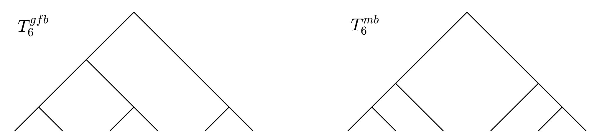
Note, however, that the maximally balanced tree on $n$ leaves is not necessarily the only tree with minimal Colless index. For example, both trees depicted in Figure 3 have minimal Colless index; one of them is the maximally balanced tree on $6$ leaves, the other one is a so-called greedy from the bottom tree, which we will introduce in the following section.

3.3.2 Greedy from the bottom trees

We now introduce another class of trees with minimal Colless index, which we call greedy from the bottom trees, or GFB trees for short. These trees can be constructed according to the following algorithm:

n\leftarrow

number of taxa; 1

treeset\leftarrow n

trees consisting of one node each; 2

min\leftarrow 1

// minimal tree size (number of leaves) in set of trees; 3

while $|treeset|>1$ do 4

u\leftarrow

tree from

treeset

of size

min

; 5

treeset=treeset\setminus\{u\}

; 6

min\leftarrow

minimal size of all trees in

treeset

; 7

v\leftarrow

tree from

treeset

of size

min

; 8

treeset=treeset\setminus\{v\}

; 9

newtree\leftarrow

tree consisting of new root

\rho_{uv}

and maximal pending subtrees

u

and

v

; 10

treeset\leftarrow treeset\cup\{newtree\}

; 11

min\leftarrow

minimal size of all trees in

treeset

; 12

end while 13

finaltree\leftarrow treeset[1]

// i.e. only remaining element of treeset; 14

return

finaltree

; 15

Algorithm 1 Greedy from the bottom

Definition 2 (GFB tree).

Let $T$ be a rooted binary tree on $n$ leaves that results from Algorithm 1. Then, $T$ is called greedy from the bottom tree or GFB tree for short and is denoted by $T^{gfb}_{n}$ .

Note that Algorithm 1 greedily clusters trees of minimal size starting with single nodes and proceeding until only one tree is left. Thus, in principle it goes from the leaves towards the root (in contrast to the greedy strategy presented in Section 3.3.1, which goes from the root towards the leaves), which is why we call the resulting trees GFB trees.

Remark 2.

Note that for $n=1$ Algorithm 1 returns one single node. Moreover, note that the GFB tree is unique for all positive integers $n$ (as it results from Algorithm 1, which is deterministic).

The following lemma shows that both maximal pending subtrees of a GFB tree are also GFB trees, which is an intuitive property and follows directly from Algorithm 1.

Lemma 5.

Let $T$ be a GFB tree with $n\geq 2$ leaves and standard decomposition $T=(T_{a},T_{b})$ . Then, $T_{a}$ and $T_{b}$ are also GFB trees.

Proof.

Let $T=(T_{a},T_{b})$ be a GFB tree and let $n_{a}$ and $n_{b}$ denote the number of leaves of $T_{a}$ and $T_{b}$ , respectively. This means that Algorithm 1 induces a bipartition of the $n$ leaves into two disjoint sets of sizes $n_{a}$ and $n_{b}$ , respectively. Note that up to the last iteration of the while-loop in Algorithm 1 these two sets are independent of each other.

Now, applying Algorithm 1 to $n_{a}$ and $n_{b}$ leaves, respectively, results in two unique GFB trees $T^{gfb}_{n_{a}}$ and $T^{gfb}_{n_{b}}$ with $n_{a}$ and $n_{b}$ leaves. As the leaf sets of $T_{a}$ and $T_{b}$ of sizes $n_{a}$ and $n_{b}$ , respectively, are independent and do not influence each other, this implies $T_{a}=T^{gfb}_{n_{a}}$ and $T_{b}=T^{gfb}_{n_{b}}$ . This completes the proof. ∎

In the following we will see that GFB trees always have minimal Colless index, even though in general the GFB tree $T_{n}^{gfb}$ is different from the maximally balanced tree $T_{n}^{mb}$ on $n$ leaves (cf. Figure 3). We can, however, characterize GFB trees in terms of the sizes of their maximal pending subtrees. This information will be very useful in subsequent analyses, in particular when showing that GFB trees have minimal Colless index (cf. Theorem 5).

Proposition 2.

Let $T_{n}^{gfb}$ be a GFB tree with $n\geq 2$ leaves and standard decomposition $T_{n}^{gfb}=(T_{a},T_{b})$ . Let $n_{a}$ and $n_{b}$ denote the number of leaves of $T_{a}$ and $T_{b}$ , respectively, such that without loss of generality, $n_{a}\geq n_{b}$ . Let $k_{n}\coloneqq\lceil\log_{2}(n)\rceil$ , i.e. $n\in(2^{k_{n}-1},2^{k_{n}}]$ . Then, we have:

1.

If $n\in(2^{k_{n}-1},3\cdot 2^{k_{n}-2})$ , we have $n_{a}=n-2^{k_{n}-2}$ and $n_{b}=2^{k_{n}-2}$ . In particular, $T_{b}$ is the fully balanced tree of height $k_{n}-2$ and we have $k_{n_{a}}\coloneqq\lceil\log_{2}(n_{a})\rceil=k_{n}-1$ .
2.

If $n=3\cdot 2^{k_{n}-2}$ , we have $n_{a}=2^{k_{n}-1}$ and $n_{b}=2^{k_{n}-2}$ . In particular, $T_{a}$ is the fully balanced tree of height $k_{n}-1$ and $T_{b}$ is the fully balanced tree of height $k_{n}-2$ .
3.

If $n\in(3\cdot 2^{k_{n}-2},2^{k_{n}}]$ , we have $n_{a}=2^{k_{n}-1}$ and $n_{b}=n-2^{k_{n}-1}$ . In particular, $T_{a}$ is the fully balanced tree of height $k_{n}-1$ and we have $k_{n_{b}}\coloneqq\lceil\log_{2}(n_{b})\rceil=k_{n}-1$ .

The proof of Proposition 2 is given in the appendix. However, it has an interesting consequence:

Corollary 1.

Let $n\in\mathbb{N}_{\geq 2}$ and $n\neq 3\cdot 2^{k_{n}-2}$ , where $k_{n}=\lceil\log_{2}(n)\rceil$ . Then, $T_{n-1}^{gfb},T_{n}^{gfb}$ and $T_{n+1}^{gfb}$ have a common maximal pending subtree, which is fully balanced:

1.

If $n\in(2^{k_{n}-1},3\cdot 2^{k_{n}-2})$ , this common subtree is a fully balanced tree of height $k_{n}-2$ .
2.

If $n\in(3\cdot 2^{k_{n}-2},2^{k_{n}}]$ , this common subtree is a fully balanced tree of height $k_{n}-1$ .

Proof.

The claimed statements are a direct consequence of Proposition 2:

1.
If $n\in(2^{k_{n}-1},3\cdot 2^{k_{n}-2})$ , we distinguish between two cases:
- (a)
  
  If $n-1>2^{k_{n}-1}$ , i.e. if $n-1$ , $n$ and $n+1$ are all in $(2^{k_{n}-1},3\cdot 2^{k_{n}-2}]$ , by Proposition 2, Parts 1 and 2, $T_{n-1}^{gfb},T_{n}^{gfb}$ and $T_{n+1}^{gfb}$ all contain a fully balanced tree of height $k_{n}-2$ as a maximal pending subtree.
- (b)
  
  If $n-1=2^{k_{n}-1}$ , by Proposition 2, Part 3, $T_{n-1}^{gfb}$ contains a fully balanced tree of height $(k_{n}-1)-1=k_{n}-2$ as a maximal pending subtree (since $k_{n-1}=\lceil\log_{2}(n-1)\rceil=\lceil\log_{2}(2^{k_{n}-1})\rceil=k_{n}-1$ ). Moreover, by Proposition 2, Part 1, $T_{n}^{gfb}$ and $T_{n+1}^{gfb}$ also contain a fully balanced tree of height $k_{n}-2$ as a maximal pending subtree.
2.
If $n\in(3\cdot 2^{k_{n}-2},2^{k_{n}}]$ , we again distinguish between two cases:
- (a)
  
  If $n\in(3\cdot 2^{k_{n}-2},2^{k_{n}})$ , then we have $n-1$ and $n+1\in[3\cdot 2^{k_{n}-2},2^{k_{n}}]$ and by Proposition 2, Parts 2 and 3, $T_{n-1}^{gfb},T_{n}^{gfb}$ and $T_{n+1}^{gfb}$ all contain a fully balanced tree of height $k_{n}-1$ as a maximal pending subtree.
- (b)
  
  If $n=2^{k_{n}}$ , then $n-1=2^{k_{n}}-1$ and $n+1=2^{k_{n}}+1$ . By Proposition 2, Part 2, $T_{n}^{gfb}$ and $T_{n-1}^{gfb}$ contain a fully balanced tree of height $k_{n}-1$ as a maximal pending subtree. Now, as $k_{n+1}=\lceil\log_{2}(n+1)\rceil=\lceil\log_{2}(2^{k_{n}}+1)\rceil=k_{n}+1$ , by Proposition 2, Part 1, $T_{n+1}^{gfb}$ contains a fully balanced tree of height $(k_{n}+1)-2=k_{n}-1$ as a maximal pending subtree. This completes the proof.

∎

We will now show that GFB trees always have minimal Colless index, i.e. we will prove the following theorem:

Theorem 5.

Let $T_{n}^{gfb}$ be a GFB tree with $n$ leaves. Then, $T_{n}^{gfb}$ has minimal Colless index, i.e. $\mathcal{C}(T_{n}^{gfb})=c_{n}$ .

In order to prove Theorem 5, we require the following technical lemma, the proof of which can be found in the Appendix.

Lemma 6.

Let $s(x)=\min\limits_{z\in\mathbb{Z}}|x-z|$ , i.e. $s(x)$ is the distance from $x$ to the nearest integer. Let $n\in\mathbb{N}$ and let $k_{n}\coloneqq\lceil\log_{2}(n)\rceil$ . Then,

1.

For $n\in(2^{k_{n}-1},3\cdot 2^{k_{n}-2}]$ , we have

$\displaystyle\frac{s(n\cdot 2^{1-k_{n}})}{2^{1-k_{n}}}$ $\displaystyle=n-2^{k_{n}-1}.$
2.

For $n\in(3\cdot 2^{k_{n}-2},2^{k_{n}}]$ , we have

$\displaystyle\frac{s(n\cdot 2^{1-k_{n}})}{2^{1-k_{n}}}$ $\displaystyle=2^{k_{n}}-n.$

We can now prove Theorem 5.

Proof of Theorem 5.

Let $T_{n}^{gfb}$ be a GFB tree with $n$ leaves. Let $k_{n}\coloneqq\lceil\log_{2}(n)\rceil$ . In order to show that $T_{n}^{gfb}$ has minimal Colless index, we show that $\mathcal{C}(T_{n}^{gfb})=c_{n}=\sum\limits_{i=0}^{k_{n}-2}\frac{s(2^{i-k_{n}+1}\cdot n)}{2^{i-k_{n}+1}}$ . We do this by induction on $n$ .

For $n=1$ we have $\mathcal{C}(T_{1}^{gfb})=0=c_{1}$ , which gives the base case of the induction.

Now, we assume that the statement given in Theorem 5 holds for all GFB trees with up to $n-1$ leaves and we show that it also holds for the GFB tree with $n$ leaves. We now distinguish between 3 cases:

$n=3\cdot 2^{k_{n}-2}$ :
By Proposition 2 we know that $T_{3\cdot 2^{k_{n}-2}}^{gfb}$ has the following standard decomposition: $T_{3\cdot 2^{k_{n}-2}}^{gfb}=(T_{k_{n}-1}^{fb},T_{k_{n}-2}^{fb})$ . In particular, both maximal pending subtrees of $T_{3\cdot 2^{k_{n}-2}}^{gfb}$ are fully balanced trees. By Theorem 3, we have $\mathcal{C}(T_{k_{n}-1}^{fb})=0$ and $\mathcal{C}(T_{k_{n}-2}^{fb})=0$ . Thus, using Lemma 1, we have

\mathcal{C}(T_{3\cdot 2^{k_{n}-2}}^{gfb})=\underbrace{\mathcal{C}(T_{k_{n}-1}^{fb})}_{=0}+\underbrace{\mathcal{C}(T_{k_{n}-2}^{fb})}_{=0}+2^{k_{n}-1}-2^{k_{n}-2}=2^{k_{n}-2}.

(13)

On the other hand,

	$\displaystyle c_{3\cdot 2^{k_{n}-2}}$	$\displaystyle=\sum\limits_{i=0}^{k_{n}-2}\frac{s(2^{i-k_{n}+1}\cdot(3\cdot 2^{k_{n}-2}))}{2^{i-k_{n}+1}}$
		$\displaystyle=\sum\limits_{i=0}^{k_{n}-2}\frac{s(3\cdot 2^{i-1})}{2^{i-k_{n}+1}}$
		$\displaystyle=\frac{s(3\cdot 2^{0-1})}{2^{0-k_{n}+1}}\;\,\text{ as }3\cdot 2^{i-1}\in\mathbb{Z}\text{ for }i>0,\text{ and thus }s(3\cdot 2^{i-1})=0\text{ for }i>0.$
		$\displaystyle=\frac{s(\frac{3}{2})}{2^{1-k_{n}}}=\frac{\frac{1}{2}}{2^{1-k_{n}}}=\frac{1}{2}\cdot 2^{k_{n}-1}=2^{k_{n}-2}=\mathcal{C}(T_{3\cdot 2^{k_{n}-2}}^{gfb})\,\text{ by }\eqref{interval_middle}.$

Thus, $T_{3\cdot 2^{k_{n}-2}}^{gfb}$ has minimal Colless index.

$n\in(2^{k_{n}-1},3\cdot 2^{k_{n}-2})$ :
By Proposition 2 we know that $T_{n}^{gfb}$ has the following standard decomposition: $T_{n}^{gfb}=(T_{n-2^{k_{n}-2}},T_{k_{n}-2}^{fb})$ . In particular, $T_{k_{n}-2}^{fb}$ is the fully balanced tree of height $k_{n}-2$ , and thus by Theorem 3, $\mathcal{C}(T_{k_{n}-2}^{fb})=0$ . Moreover, for $T_{n-2^{k_{n}-2}}$ we have: $\lceil\log_{2}(n-2^{k_{n}-2})\rceil=k_{n}-1$ . Thus, using Lemma 1 and Lemma 2, we have

	$\displaystyle\mathcal{C}(T_{n}^{gfb})$	$\displaystyle=\mathcal{C}(T_{n-2^{k_{n}-2}})+\underbrace{\mathcal{C}(T_{k_{n}-2}^{fb})}_{=0}+(n-2^{k_{n}-2})-2^{k_{n}-2}$
		$\displaystyle=\mathcal{C}(T_{n-2^{k_{n}-2}}^{gfb})+n-2^{k_{n}-1}\;\text{ by Lemma \ref{gfb_subtrees}}$
		$\displaystyle=c_{n-2^{k_{n}-2}}+n-2^{k_{n}-1}\;\text{ by the inductive hypothesis}$
		$\displaystyle=\sum\limits_{i=0}^{(k_{n}-1)-2}\frac{s(2^{i-(k_{n}-1)+1}\cdot(n-2^{k_{n}-2}))}{2^{i-(k_{n}-1)+1}}+n-2^{k_{n}-1}\;\text{ by Theorem \ref{colless_explicit}}$
		$\displaystyle=\sum\limits_{i=0}^{k_{n}-3}\frac{s(2^{i-k_{n}+2}\cdot(n-2^{k_{n}-2}))}{2^{i-k_{n}+2}}+n-2^{k_{n}-1}$
		$\displaystyle=\sum\limits_{i=0}^{k_{n}-3}\frac{s(2^{i-k_{n}+2}\cdot n-2^{i})}{2^{i-k_{n}+2}}+n-2^{k_{n}-1}$
		$\displaystyle=\sum\limits_{i=0}^{k_{n}-3}\frac{s(2^{i-k_{n}+2}\cdot n)}{2^{i-k_{n}+2}}+n-2^{k_{n}-1}\,\text{ by Lemma \ref{subbaditivity_of_s}, Part 2, as }2^{i}\in\mathbb{Z}$
		$\displaystyle=\frac{s(2^{2-k_{n}}\cdot n)}{2^{2-k_{n}}}+\frac{s(2^{3-k_{n}}\cdot n)}{2^{3-k_{n}}}+\ldots+\frac{s(2^{-1}\cdot n)}{2^{-1}}+n-2^{k_{n}-1}$
		$\displaystyle=\frac{s(2^{1-k_{n}}\cdot n)}{2^{1-k_{n}}}+\frac{s(2^{2-k_{n}}\cdot n)}{2^{2-k_{n}}}+\frac{s(2^{3-k_{n}}\cdot n)}{2^{3-k_{n}}}+\ldots+\frac{s(2^{-1}\cdot n)}{2^{-1}}$
		$\displaystyle\text{ as }n-2^{k_{n}-1}=\frac{s(2^{1-k_{n}}\cdot n)}{2^{1-k_{n}}}\text{ by Lemma \ref{gfb_technical_lemma}, Part 1}.$
		$\displaystyle=\sum\limits_{i=0}^{k_{n}-2}\frac{s(2^{i-k_{n}+1}\cdot n)}{2^{i-k_{n}+1}}=c_{n}\,\text{ by Theorem \ref{colless_explicit}.}$

Thus, $T_{n}^{gfb}$ has minimal Colless index.

3.

$n\in(3\cdot 2^{k_{n}-2},2^{k_{n}}]$ :
This case follows analogously to the previous case, but instead of using Part 1 of Lemma 6, we use Part 2. For completeness the proof can be found in the Appendix.

Thus, in all cases, $\mathcal{C}(T_{n}^{gfb})=c_{n}$ , which completes the proof. ∎

Note that for $n=2^{k_{n}}$ Theorem 5 together with Theorem 3 implies that $T^{gfb}_{2^{k_{n}}}=T^{fb}_{k_{n}}$ .

3.3.3 Further characterizing and counting trees with minimal Colless index

So far, we have seen that there are two classes of trees with minimal Colless index, namely maximally balanced trees and GFB trees. However, there are trees that are neither maximally balanced nor GFB, but still have minimal Colless index (e.g. tree $T_{1}$ depicted in Figure 4). In the following, we will thus try to further characterize and count trees with minimal Colless index.

In particular, we will show that the leaf partitioning of $n$ leaves into $n_{a}$ and $n_{b}$ as induced by Algorithm 1 is the most extreme one a tree with minimal Colless index can have. This means that given a tree $T$ with minimal Colless index, the difference in the number of leaves of its two maximal pending subtrees $n_{a}-n_{b}$ cannot be larger than it is in a GFB tree. To be precise, we have the following theorem:

Theorem 6.

Let $T^{gfb}_{n}=(T_{a},T_{b})$ be a GFB tree on $n$ leaves with $n\in(2^{k_{n}-1},2^{k_{n}})$ (where $k_{n}=\lceil\log_{2}(n)\rceil$ ), i.e.

(n_{a},n_{b})=\begin{cases}(n-2^{k_{n}-2},2^{k_{n}-2}),&\text{ if }n\in(2^{k_{n}-1},3\cdot 2^{k_{n}-2});\\ (2^{k_{n}-1},2^{k_{n}-2}),&\text{ if }n=3\cdot 2^{k_{n}-2};\\ (2^{k_{n}-1},n-2^{k_{n}-1}),&\text{ if }n\in(3\cdot 2^{k_{n}-2},2^{k_{n}}),\end{cases}

where we have $n_{a}-n_{b}=n-2^{k_{n}-1}$ in the first case, $n_{a}-n_{b}=2^{k_{n}-2}$ in the second case and $n_{a}-n_{b}=2^{k_{n}}-n$ in the last case. Now, suppose that $\widehat{T}=(\widehat{T}_{a},\widehat{T}_{b})$ is a tree with a more extreme leaf partitioning, i.e. $\widehat{n}_{a}-\widehat{n}_{b}>n_{a}-n_{b}$ or, to be more precise,

(\widehat{n}_{a},\widehat{n}_{b})=\begin{cases}(n-2^{k_{n}-2}+j,2^{k_{n}-2}-j)\text{ with }j\in\{1,\ldots,2^{k_{n}-2}-1\},&\text{ if }n\in(2^{k_{n}-1},3\cdot 2^{k_{n}-2});\\ (2^{k_{n}-1}+j,2^{k_{n}-2}-j)\text{ with }j\in\{1,\ldots,2^{k_{n}-2}-1\},&\text{ if }n=3\cdot 2^{k_{n}-2};\\ (2^{k_{n}-1}+j,n-2^{k_{n}-1}-j)\text{ with }j\in\{1,\ldots,n-2^{k_{n}-1}-1\},&\text{ if }n\in(3\cdot 2^{k_{n}-2},2^{k_{n}}).\end{cases}

Then, we have

c_{n}=\mathcal{C}(T^{gfb}_{n})<\mathcal{C}(\widehat{T}),

i.e. $\widehat{T}$ does not have minimal Colless index (where the first equality follows from Theorem 5).

The proof of this theorem requires the following lemma, which provides an upper bound on the maximal minimal Colless index for any given $n\in(2^{k_{n}-1},2^{k_{n}})$ . This upper bound is also depicted in Figure 2.

Lemma 7.

Let $n\in(2^{k_{n}-1},2^{k_{n}})$ with $k_{n}=\lceil\log_{2}(n)\rceil$ . Let $\bar{c}_{n}$ denote the maximal minimal Colless index for $n\in(2^{k_{n}-1},2^{k_{n}})$ , i.e.

\bar{c}_{n}=\max\limits_{n\in(2^{k_{n}-1},2^{k_{n}})}c_{n}.

Then, we have

\bar{c}_{n}<2^{k_{n}-1}.

Proof.

By Theorem 2, we have for the minimal Colless index

	$\displaystyle c_{n}$	$\displaystyle=\sum\limits_{i=0}^{k_{n}-2}\frac{s(2^{i-k_{n}+1}\cdot n)}{2^{i-k_{n}+1}}$
		$\displaystyle=\frac{s(2^{1-k_{n}}\cdot n)}{2^{1-k_{n}}}+\frac{s(2^{2-k_{n}}\cdot n)}{2^{2-k_{n}}}+\ldots+\frac{s(2^{-2}\cdot n)}{2^{-2}}+\frac{s(2^{-1}\cdot n)}{2^{-1}}$
		$\displaystyle\leq\frac{\frac{1}{2}}{2^{1-k_{n}}}+\frac{\frac{1}{2}}{2^{2-k_{n}}}+\ldots+\frac{\frac{1}{2}}{2^{-2}}+\frac{\frac{1}{2}}{2^{-1}},\,\text{ as }s(x)=\min\limits_{z\in\mathbb{Z}}\|x-z\|\leq\frac{1}{2}\,\forall x$
		$\displaystyle=\sum\limits_{m=0}^{k_{n}-2}2^{m}=\sum\limits_{m=0}^{k_{n}}2^{m}-2^{k_{n}-1}-2^{k_{n}}=(2^{k_{n}+1}-1)-2^{k_{n}-1}-2^{k_{n}}$
		$\displaystyle=2^{k_{n}-1}-1<2^{k_{n}-1}.$

This means that $c_{n}$ is bounded from above by $2^{k_{n}-1}$ . In particular, $\bar{c}_{n}=\max\limits_{n\in(2^{k_{n}-1},2^{k_{n}})}c_{n}<2^{k_{n}-1}$ , which completes the proof. ∎

We are now in a position to prove Theorem 6, which is divided into three subcases. For $n=3\cdot 2^{k_{n}-2}$ the proof is straightforward, while the cases $n\in(2^{k_{n}-1},3\cdot 2^{k_{n}-2})$ and $n\in(3\cdot 2^{k_{n}-2},2^{k_{n}})$ are more technical and require Lemma 3 and Lemma 7.

Proof of Theorem 6.

Let $n\in(2^{k_{n}-1},2^{k_{n}})$ with $k_{n}=\lceil\log_{2}(n)\rceil$ . Let $T^{gfb}_{n}=(T_{a},T_{b})$ be the GFB tree on $n$ leaves. We now distinguish between three cases (only case 1. is given here; the other two cases are shown in the Appendix):

$n\in(2^{k_{n}-1},3\cdot 2^{k_{n}-2})$ :
From Proposition 2, we have for $T^{gfb}_{n}=(T_{a},T_{b})$ that $n_{a}=n-2^{k_{n}-2}$ and $n_{b}=2^{k_{n}-2}$ . In particular, $T_{b}$ is the fully balanced tree of height $k_{n}-2$ and we have $\mathcal{C}(T_{b})=c_{n_{b}}=0$ by Theorem 3. For $T_{a}$ we have $k_{n_{a}}=\lceil\log_{2}(n_{a})\rceil=k_{n}-1$ . Now, consider $\mathcal{C}(T^{gfb}_{n})$ . By Lemmas 1 and 2 and by Theorem 5 we have

$\displaystyle\mathcal{C}(T^{gfb}_{n})$	$\displaystyle=n_{a}-n_{b}+c_{n_{a}}+c_{n_{b}}$
	$\displaystyle=n_{a}-n_{b}+c_{n_{a}}$	(14)
	$\displaystyle=n_{a}-n_{b}+c_{n-2^{k_{n}-2}}$
	$\displaystyle=n_{a}-n_{b}+\sum\limits_{i=0}^{k_{n}-3}\frac{s(2^{i-k_{n}+2}\cdot(n-2^{k_{n}-2}))}{2^{i-k_{n}+2}}$
	$\displaystyle=n_{a}-n_{b}+\sum\limits_{i=0}^{k_{n}-3}\frac{s(2^{i-k_{n}+2}\cdot n-2^{i})}{2^{i-k_{n}+2}}$
	$\displaystyle=n_{a}-n_{b}+\sum\limits_{i=0}^{k_{n}-3}\frac{s(2^{i-k_{n}+2}\cdot n)}{2^{i-k_{n}+2}}\,\text{ by Lemma \ref{subbaditivity_of_s}, Part 2, as }2^{i}\in\mathbb{Z}$
	$\displaystyle=n_{a}-n_{b}+\sum\limits_{i=0}^{k_{n}-3}\frac{s(2^{i-k_{n}+2}\cdot((n+j)-j))}{2^{i-k_{n}+2}}$
	$\displaystyle=n_{a}-n_{b}+\sum\limits_{i=0}^{k_{n}-3}\frac{s(2^{i-k_{n}+2}\cdot(n+j)+2^{i-k_{n}+2}\cdot(-j))}{2^{i-k_{n}+2}}.$	(15)

Now, suppose that $\widehat{T}=(\widehat{T}_{a},\widehat{T}_{b})$ with $\widehat{n}_{a}=n_{a}+j$ and $\widehat{n}_{b}=n_{b}-j$ (and $j\in\{1,\ldots,2^{k_{n}-2}-1\}$ ) is also a tree with minimal Colless index, i.e. $\mathcal{C}(\widehat{T})=\mathcal{C}(T^{gfb}_{n})=c_{n}$ . Consider $\mathcal{C}(\widehat{T})$ . Again, by Lemmas 1 and 2, we have

$\displaystyle\mathcal{C}(\widehat{T})$	$\displaystyle=\widehat{n}_{a}-\widehat{n}_{b}+c_{\widehat{n}_{a}}+c_{\widehat{n}_{b}}$
	$\displaystyle=(n_{a}+j)-(n_{b}-j)+c_{\widehat{n}_{a}}+c_{\widehat{n}_{b}}$
	$\displaystyle=n_{a}-n_{b}+2j+c_{\widehat{n}_{a}}+c_{\widehat{n}_{b}}$
	$\displaystyle=n_{a}-n_{b}+2j+\underbrace{c_{n-2^{k_{n}-2}+j}}_{\geq 0}+\underbrace{c_{2^{k_{n}-2}-j}}_{\geq 0}.$	(16)

Now, comparing $\mathcal{C}(T^{gfb}_{n})$ (see Equation (14)) and $\mathcal{C}(\widehat{T})$ (see Equation (16)) it immediately follows that we have $\mathcal{C}(T^{gfb}_{n})<\mathcal{C}(\widehat{T})$ if $c_{n_{a}}<2j$ , which would contradict the minimality of $\mathcal{C}(\widehat{T})$ . Thus, we have $c_{n_{a}}\geq 2j$ . We now claim that $c_{n_{a}}\geq 2j$ implies $k_{\widehat{n}_{b}}=\lceil\log_{2}(\widehat{n}_{b})\rceil=k_{n_{b}}=k_{n}-2$ . To see this, consider the following:

(a)

As $\widehat{n}_{b}<n_{b}$ , we have $k_{\widehat{n}_{b}}\leq k_{n_{b}}=k_{n}-2$ .
(b)

Suppose $k_{\widehat{n}_{b}}\leq k_{n}-3$ . As $\widehat{n}_{b}=n_{b}-j=2^{k_{n}-2}-j$ , this implies $j\geq 2^{k_{n}-3}$ . In particular, $2j\geq 2^{k_{n}-2}$ .
Now, consider $c_{n_{a}}$ . As $k_{n_{a}}=k_{n}-1$ it follows from Lemma 7 that

$\displaystyle c_{n_{a}}<2^{(k_{n}-1)-1}=2^{k_{n}-2}.$

However, as $2j\geq 2^{k_{n}-2}$ , this implies $c_{n_{a}}<2j$ , which contradicts the assumption that $c_{n_{a}}\geq 2j$ . Thus, $k_{\widehat{n}_{b}}>k_{n}-3$ .

Thus, in total we have $k_{\widehat{n_{b}}}=k_{n}-2$ . This, however, implies that

j\leq 2^{k_{n}-3}-1<2^{k_{n}-3}=\frac{1}{2}\cdot 2^{k_{n}-2}.

In particular, $j\in(0\cdot 2^{k_{n}-2},\frac{1}{2}\cdot 2^{k_{n}-2})$ and $2^{2-k_{n}}\cdot j\in(0,\frac{1}{2})$ . This, in turn, implies

\displaystyle\frac{s(2^{2-k_{n}}\cdot(-j))}{2^{2-k_{n}}}

\displaystyle=\frac{s(2^{2-k_{n}}\cdot j)}{2^{2-k_{n}}}=\frac{2^{2-k_{n}}\cdot j}{2^{2-k_{n}}}=j,

(17)

a fact that will be used later on.

Moreover, we have for $\widehat{T}_{a}$ : $k_{\widehat{n}_{a}}=\lceil\log_{2}(\widehat{n}_{a})\rceil\in\{k_{n}-1,k_{n}\}$ :

(a)

As $\widehat{n}_{a}>n_{a}$ and $k_{n_{a}}=k_{n}-1$ , it follows that $k_{\widehat{n}_{a}}\geq k_{n}-1$ .
(b)

However, as $\widehat{n}_{a}<n$ , it also follows that $k_{\widehat{n}_{a}}\leq k_{n}$ .

In total $k_{\widehat{n}_{a}}\in\{k_{n}-1,k_{n}\}$ .

Thus, for $\widehat{T}$ we now distinguish between two cases:

(a)

$k_{\widehat{n}_{a}}=k_{n}-1$ and $k_{\widehat{n}_{b}}=k_{n}-2$ :
Continuing from Equation (16) and using Theorem 2, we have

$\displaystyle\mathcal{C}(\widehat{T})$	$\displaystyle=n_{a}-n_{b}+2j+c_{n-2^{k_{n}-2}+j}+c_{2^{k_{n}-2}-j}$
	$\displaystyle=n_{a}-n_{b}+2j+\sum\limits_{i=0}^{k_{n}-3}\frac{s(2^{i-k_{n}+2}\cdot(n-2^{k_{n}-2}+j))}{2^{i-k_{n}+2}}+\sum\limits_{i=0}^{k_{n}-4}\frac{s(2^{i-k_{n}+3}\cdot(2^{k_{n}-2}-j))}{2^{i-k_{n}+3}}$
	$\displaystyle=n_{a}-n_{b}+2j+\sum\limits_{i=0}^{k_{n}-3}\frac{s(2^{i-k_{n}+2}\cdot(n+j)-2^{i})}{2^{i-k_{n}+2}}+\sum\limits_{i=0}^{k_{n}-4}\frac{s(2^{i+1}-2^{i-k_{n}+3}\cdot j)}{2^{i-k_{n}+3}}$
	$\displaystyle\text{ by Lemma \ref{subbaditivity_of_s}, Part 2, as }2^{i}\text{ and }2^{i+1}\in\mathbb{Z}$
	$\displaystyle=n_{a}-n_{b}+2j+\sum\limits_{i=0}^{k_{n}-3}\frac{s(2^{i-k_{n}+2}\cdot(n+j))}{2^{i-k_{n}+2}}+\sum\limits_{i=0}^{k_{n}-4}\frac{s(2^{i-k_{n}+3}\cdot(-j))}{2^{i-k_{n}+3}}$
	$\displaystyle=n_{a}-n_{b}+2j+\sum\limits_{i=0}^{k_{n}-3}\frac{s(2^{i-k_{n}+2}\cdot(n+j))}{2^{i-k_{n}+2}}+\sum\limits_{i=1}^{k_{n}-3}\frac{s(2^{i-k_{n}+2}\cdot(-j))}{2^{i-k_{n}+2}}$
	$\displaystyle=n_{a}-n_{b}+2j+\sum\limits_{i=0}^{k_{n}-3}\frac{s(2^{i-k_{n}+2}\cdot(n+j))}{2^{i-k_{n}+2}}+\sum\limits_{i=0}^{k_{n}-3}\frac{s(2^{i-k_{n}+2}\cdot(-j))}{2^{i-k_{n}+2}}-\frac{s(2^{2-k_{n}}\cdot(-j))}{2^{2-k_{n}}}$
	$\displaystyle=n_{a}-n_{b}+2j+\sum\limits_{i=0}^{k_{n}-3}\frac{s(2^{i-k_{n}+2}\cdot(n+j))}{2^{i-k_{n}+2}}+\sum\limits_{i=0}^{k_{n}-3}\frac{s(2^{i-k_{n}+2}\cdot(-j))}{2^{i-k_{n}+2}}-j\,\text{ by }\eqref{j}$
	$\displaystyle=n_{a}-n_{b}+j+\sum\limits_{i=0}^{k_{n}-3}\frac{s(2^{i-k_{n}+2}\cdot(n+j))}{2^{i-k_{n}+2}}+\sum\limits_{i=0}^{k_{n}-3}\frac{s(2^{i-k_{n}+2}\cdot(-j))}{2^{i-k_{n}+2}}.$	(18)

Now, as by assumption both $T^{gfb}_{n}$ and $\widehat{T}$ are trees with minimal Colless index, we have (using Equations (15) and (18))

	$\displaystyle 0$	$\displaystyle=\mathcal{C}(T^{gfb}_{n})-\mathcal{C}(\widehat{T})$
		$\displaystyle=n_{a}-n_{b}+\sum\limits_{i=0}^{k_{n}-3}\frac{s(2^{i-k_{n}+2}\cdot(n+j)+2^{i-k_{n}+2}\cdot(-j))}{2^{i-k_{n}+2}}$
		$\displaystyle\hskip 14.22636pt-n_{a}+n_{b}-j-\sum\limits_{i=0}^{k_{n}-3}\frac{s(2^{i-k_{n}+2}\cdot(n+j))}{2^{i-k_{n}+2}}-\sum\limits_{i=0}^{k_{n}-3}\frac{s(2^{i-k_{n}+2}\cdot(-j))}{2^{i-k_{n}+2}}$
		$\displaystyle=\sum\limits_{i=0}^{k_{n}-3}\underbrace{\frac{s(2^{i-k_{n}+2}\cdot(n+j)+2^{i-k_{n}+2}\cdot(-j))-\big(s(2^{i-k_{n}+2}\cdot(n+j))+s(2^{i-k_{n}+2}\cdot(-j))\big)}{2^{i-k_{n}+2}}}_{\leq 0\text{ by Lemma \ref{subbaditivity_of_s}, Part 1}}-j$
		$\displaystyle<0.$

This, however, is a contradiction. Thus, $\mathcal{C}(\widehat{T})$ is not minimal, which completes the proof for this subcase.

(b)

$k_{\widehat{n}_{a}}=k_{n}$ and $k_{\widehat{n}_{b}}=k_{n}-2$ :
Again, continuing from Equation (16) and using Theorem 2, we have

$\displaystyle\mathcal{C}(\widehat{T})$	$\displaystyle=n_{a}-n_{b}+2j+c_{n-2^{k_{n}-2}+j}+c_{2^{k_{n}-2}-j}$
	$\displaystyle=n_{a}-n_{b}+2j+\sum\limits_{i=0}^{k_{n}-2}\frac{s(2^{i-k_{n}+1}\cdot(n-2^{k_{n}-2}+j))}{2^{i-k_{n}+1}}+\sum\limits_{i=0}^{k_{n}-4}\frac{s(2^{i-k_{n}+3}\cdot(2^{k_{n}-2}-j))}{2^{i-k_{n}+3}}$
	$\displaystyle=n_{a}-n_{b}+2j+\sum\limits_{i=0}^{k_{n}-2}\frac{s(2^{i-k_{n}+1}\cdot(n+j)-2^{i-1})}{2^{i-k_{n}+1}}+\sum\limits_{i=0}^{k_{n}-4}\frac{s(2^{i+1}+2^{i-k_{n}+3}\cdot(-j))}{2^{i-k_{n}+3}}$
	$\displaystyle=n_{a}-n_{b}+2j+\sum\limits_{i=0}^{k_{n}-2}\frac{s(2^{i-k_{n}+1}\cdot(n+j)-2^{i-1})}{2^{i-k_{n}+1}}+\sum\limits_{i=0}^{k_{n}-4}\frac{s(2^{i-k_{n}+3}\cdot(-j))}{2^{i-k_{n}+3}}$
	$\displaystyle\text{ by Lemma \ref{subbaditivity_of_s}, Part 2, as }2^{i+1}\in\mathbb{Z}$
	$\displaystyle=n_{a}-n_{b}+2j+\frac{s(2^{1-k_{n}}\cdot(n+j)-2^{-1})}{2^{1-k_{n}}}+\sum\limits_{i=1}^{k_{n}-2}\frac{s(2^{i-k_{n}+1}\cdot(n+j)-2^{i-1})}{2^{i-k_{n}+1}}$
	$\displaystyle\hskip 14.22636pt+\sum\limits_{i=0}^{k_{n}-4}\frac{s(2^{i-k_{n}+3}\cdot(-j))}{2^{i-k_{n}+3}}$
	$\displaystyle=n_{a}-n_{b}+2j+\frac{s(2^{1-k_{n}}\cdot(n+j)-2^{-1})}{2^{1-k_{n}}}+\sum\limits_{i=0}^{k_{n}-3}\frac{s(2^{i-k_{n}+2}\cdot(n+j)-2^{i})}{2^{i-k_{n}+2}}$
	$\displaystyle\hskip 14.22636pt+\sum\limits_{i=0}^{k_{n}-4}\frac{s(2^{i-k_{n}+3}\cdot(-j))}{2^{i-k_{n}+3}}$
	$\displaystyle=n_{a}-n_{b}+2j+\frac{s(2^{1-k_{n}}\cdot(n+j)-2^{-1})}{2^{1-k_{n}}}+\sum\limits_{i=0}^{k_{n}-3}\frac{s(2^{i-k_{n}+2}\cdot(n+j))}{2^{i-k_{n}+2}}$
	$\displaystyle\hskip 14.22636pt+\sum\limits_{i=0}^{k_{n}-4}\frac{s(2^{i-k_{n}+3}\cdot(-j))}{2^{i-k_{n}+3}}\text{ by Lemma \ref{subbaditivity_of_s}, Part 2, as }2^{i}\in\mathbb{Z}$
	$\displaystyle=n_{a}-n_{b}+2j+\frac{s(2^{1-k_{n}}\cdot(n+j)-2^{-1})}{2^{1-k_{n}}}+\sum\limits_{i=0}^{k_{n}-3}\frac{s(2^{i-k_{n}+2}\cdot(n+j))}{2^{i-k_{n}+2}}$
	$\displaystyle\hskip 14.22636pt+\sum\limits_{i=1}^{k_{n}-3}\frac{s(2^{i-k_{n}+2}\cdot(-j))}{2^{i-k_{n}+2}}$
	$\displaystyle=n_{a}-n_{b}+2j+\frac{s(2^{1-k_{n}}\cdot(n+j)-2^{-1})}{2^{1-k_{n}}}+\sum\limits_{i=0}^{k_{n}-3}\frac{s(2^{i-k_{n}+2}\cdot(n+j))}{2^{i-k_{n}+2}}$
	$\displaystyle\hskip 14.22636pt+\sum\limits_{i=0}^{k_{n}-3}\frac{s(2^{i-k_{n}+2}\cdot(-j))}{2^{i-k_{n}+2}}-\frac{s(2^{2-k_{n}}\cdot(-j))}{2^{2-k_{n}}}$
	$\displaystyle=n_{a}-n_{b}+2j+\frac{s(2^{1-k_{n}}\cdot(n+j)-2^{-1})}{2^{1-k_{n}}}+\sum\limits_{i=0}^{k_{n}-3}\frac{s(2^{i-k_{n}+2}\cdot(n+j))}{2^{i-k_{n}+2}}$
	$\displaystyle\hskip 14.22636pt+\sum\limits_{i=0}^{k_{n}-3}\frac{s(2^{i-k_{n}+2}\cdot(-j))}{2^{i-k_{n}+2}}-j\,\text{ by }\eqref{j}.$	(19)

Again, as by assumption both $T^{gfb}_{n}$ and $\widehat{T}$ are trees with minimal Colless index, we have (using Equations (15) and (19))

	$\displaystyle 0$	$\displaystyle=\mathcal{C}(T^{gfb}_{n})-\mathcal{C}(\widehat{T})$
		$\displaystyle=n_{a}-n_{b}+\sum\limits_{i=0}^{k_{n}-3}\frac{s(2^{i-k_{n}+2}\cdot(n+j)+2^{i-k_{n}+2}\cdot(-j))}{2^{i-k_{n}+2}}$
		$\displaystyle\hskip 14.22636pt-n_{a}+n_{b}-j-\frac{s(2^{1-k_{n}}\cdot(n+j)-2^{-1})}{2^{1-k_{n}}}-\sum\limits_{i=0}^{k_{n}-3}\frac{s(2^{i-k_{n}+2}\cdot(n+j))}{2^{i-k_{n}+2}}$
		$\displaystyle\hskip 14.22636pt-\sum\limits_{i=0}^{k_{n}-3}\frac{s(2^{i-k_{n}+2}\cdot(-j))}{2^{i-k_{n}+2}}$
		$\displaystyle=\sum\limits_{i=0}^{k_{n}-3}\underbrace{\frac{s(2^{i-k_{n}+2}\cdot(n+j)+2^{i-k_{n}+2}\cdot(-j))-\big(s(2^{i-k_{n}+2}\cdot(n+j))+s(2^{i-k_{n}+2}\cdot(-j))\big)}{2^{i-k_{n}+2}}}_{\leq 0\text{ by Lemma \ref{subbaditivity_of_s}, Part 1}}$
		$\displaystyle\hskip 14.22636pt-\underbrace{j}_{>0}-\underbrace{\frac{s(2^{1-k_{n}}\cdot(n+j)-2^{-1})}{2^{1-k_{n}}}}_{\geq 0}$
		$\displaystyle<0.$

This, however, is a contradiction. Thus, $\mathcal{C}(\widehat{T})$ is not minimal, which completes the proof for this subcase.

For $n=3\cdot 2^{k_{n}-2}$ the proof is straightforward and for $n\in(3\cdot 2^{k_{n}-2},2^{k_{n}})$ the proof is similar to the case shown above. Thus, both cases are given in the Appendix.

In all cases, we have $\mathcal{C}(\widehat{T})>\mathcal{C}(T^{gfb}_{n})$ , which completes the proof. ∎

To summarize, we have seen that both maximally balanced trees and GFB trees have minimal Colless index (cf. Theorems 4 and 5). Moreover, for a tree $T=(T_{a},T_{b})$ with minimal Colless index we always have:

Corollary 2.

Let $T=(T_{a},T_{b})$ be a tree on $n$ leaves with minimal Colless index, i.e. $\mathcal{C}(T)=c_{n}$ . Let $n_{a},n_{b}$ denote the number of leaves of $T_{a}$ and $T_{b}$ , respectively, where $n_{a}\geq n_{b}$ . Then

	$\displaystyle n_{a}^{gfb}$	$\displaystyle\geq n_{a}\geq n_{a}^{mb}$
	$\displaystyle n_{b}^{gfb}$	$\displaystyle\leq n_{b}\leq n_{b}^{mb},$

where $n_{a}^{gfb}$ and $n_{b}^{gfb}$ denote the number of leaves of $T^{gfb}_{a}$ and $T^{gfb}_{b}$ in $T_{n}^{gfb}=(T_{a}^{gfb},T_{b}^{gfb})$ and $n_{a}^{mb}$ and $n_{b}^{mb}$ denote the number of leaves of $T_{a}^{mb}$ and $T_{b}^{mb}$ in $T_{n}^{mb}=(T_{a}^{mb},T_{b}^{mb})$ .

Proof.

Now, recall that both maximally balanced trees and GFB trees have minimal Colless index (cf. Theorems 4 and 5).

Assume $n_{a}<n_{a}^{mb}$ and $n_{b}>n_{b}^{mb}$ . As $n_{a}^{mb}=n_{b}^{mb}=\frac{n}{2}$ for $n$ even and $n_{a}^{mb}=\frac{n+1}{2}$ and $n_{b}^{mb}=\frac{n-1}{2}$ for $n$ odd, this assumption contradicts $n_{a}\geq n_{b}$ . Thus, $n_{a}\geq n_{a}^{mb}$ and $n_{b}\leq n_{b}^{mb}$ .

Additionally, $n_{a}\leq n_{a}^{gfb}$ and $n_{b}\geq n_{b}^{gfb}$ is a direct consequence of Theorem 6. This completes the proof. ∎

Note that Corollary 2 only gives a necessary and not a sufficient condition. Consider for example tree $T_{2}$ in Figure 4 on $12$ leaves. Here, $n_{a}=7$ and $n_{b}=5$ , i.e.

	$\displaystyle n_{a}^{gfb}=8$	$\displaystyle\geq 7\geq 6=n_{a}^{mb}$
	$\displaystyle n_{b}^{gfb}=4$	$\displaystyle\leq 5\leq 6=n_{b}^{mb},$

but $T_{2}$ does not have minimal Colless index. This is due to the fact that if $n_{a}\neq n_{b}$ and $n_{b},n_{b}$ odd, the resulting tree will not have minimal Colless index:

Theorem 7.

Let $T=(T_{a},T_{b})$ be a tree on $n$ leaves and let $n_{a}$ and $n_{b}$ denote the number of leaves of $T_{a}$ and $T_{b}$ . If $n_{a}\neq n_{b}$ and $n_{a},n_{b}$ odd, then $C(T)>c_{n}$ , i.e. $T$ does not have minimal Colless index.

Proof.

Let $T=(T_{a},T_{b})$ be a tree on $n$ leaves. Let $n_{a}$ and $n_{b}$ denote the number of leaves of $T_{a}$ and $T_{b}$ with $n_{a}\neq n_{b}$ and $n_{a},n_{b}$ odd. Without loss of generality let $n_{a}>n_{b}$ . The fact that $n_{a}$ and $n_{b}$ are both odd, results in

	$\displaystyle n_{a}$	$\displaystyle\geq n_{b}+2$
	$\displaystyle\Leftrightarrow\frac{n_{a}-1}{2}$	$\displaystyle\geq\frac{n_{b}+1}{2}.$		(20)

By (20) we also have

\displaystyle\frac{n_{a}+1}{2}

\displaystyle>\frac{n_{b}+1}{2}.

(21)

We prove the statement by contradiction and assume that $C(T)=c_{n}$ , i.e. $T$ has minimal Colless index. Then,

$\displaystyle c_{n}$	$\displaystyle=c_{n_{a}}+c_{n_{b}}+n_{a}-n_{b}\quad\text{by Lemma }\ref{colless_sum}\text{ and Lemma }\ref{max_subtrees}$
	$\displaystyle=c_{\frac{n_{a}+1}{2}}+c_{\frac{n_{a}-1}{2}}+1+c_{\frac{n_{b}+1}{2}}+c_{\frac{n_{b}-1}{2}}+1+n_{a}-n_{b}\quad\text{by Theorem }\ref{colless_minimum}$
	$\displaystyle=c_{\frac{n_{a}+1}{2}}+c_{\frac{n_{a}-1}{2}}+c_{\frac{n_{b}+1}{2}}+c_{\frac{n_{b}-1}{2}}+n_{a}-n_{b}+2.$	(22)

Additionally, by Lemma 1, Lemma 2 and (21)

\displaystyle c_{\frac{n}{2}}=c_{\frac{n_{a}+n_{b}}{2}}\leq c_{\frac{n_{a}+1}{2}}+c_{\frac{n_{b}-1}{2}}+\frac{n_{a}+1}{2}-\frac{n_{b}-1}{2},

which results in

\displaystyle c_{\frac{n}{2}}-\frac{n_{a}-n_{b}}{2}-1\leq c_{\frac{n_{a}+1}{2}}+c_{\frac{n_{b}-1}{2}}.

(23)

Similarly, by Lemma 1, Lemma 2 and (20)

\displaystyle c_{\frac{n}{2}}=c_{\frac{n_{a}+n_{b}}{2}}\leq c_{\frac{n_{a}-1}{2}}+c_{\frac{n_{b}+1}{2}}+\frac{n_{a}-1}{2}-\frac{n_{b}+1}{2},

which results in

\displaystyle c_{\frac{n}{2}}-\frac{n_{a}-n_{b}}{2}+1\leq c_{\frac{n_{a}-1}{2}}+c_{\frac{n_{b}+1}{2}}.

(24)

By (23) and (24) and the fact that $n$ is even we can rewrite (22) in the following way

	$\displaystyle c_{n}$	$\displaystyle=c_{\frac{n_{a}+1}{2}}+c_{\frac{n_{a}-1}{2}}+c_{\frac{n_{b}+1}{2}}+c_{\frac{n_{b}-1}{2}}+n_{a}-n_{b}+2$
		$\displaystyle\geq c_{\frac{n}{2}}-\frac{n_{a}-n_{b}}{2}-1+c_{\frac{n}{2}}-\frac{n_{a}-n_{b}}{2}+1+n_{a}-n_{b}+2$
		$\displaystyle=2c_{\frac{n}{2}}+2$
		$\displaystyle=c_{n}+2\quad\text{by Theorem }\ref{colless_minimum}.$

This results in $c_{n}\geq c_{n}+2$ which is a contradiction, and therefore completes the proof. ∎

Thus, if $n_{a}\neq n_{b}$ , and $n_{a},n_{b}$ odd, the resulting tree does not have minimal Colless index. However, it can easily be verified that if $n_{a}\neq n_{b}$ , but both $n_{a}$ and $n_{b}$ are even, the resulting tree may or may not have minimal Colless index. Consider for example $n=24$ : In this case $\lceil\log_{2}(24)\rceil=5$ and thus by Theorem 2 we have:

	$\displaystyle c_{24}$	$\displaystyle=\sum\limits_{i=0}^{3}\frac{s(2^{i-4}\cdot 24)}{2^{i-4}}=8$
		$\displaystyle=c_{16}+c_{8}+8=0+0+8$
		$\displaystyle<c_{14}+c_{10}+4=4+4+4=12.$

Thus, while $n_{a}=16,n_{b}=8$ yields a Colless minimum, $n_{a}=14,n_{b}=10$ does not.

We now turn to the number of trees on $n$ leaves with minimal Colless index and state an upper bound for it. This bound is implied by the fact that we can relate trees with minimal Colless index with trees with minimal Sackin index, another index of tree balance which is defined as follows:

Definition 3 (Sackin 1972).

Let $T$ be a rooted binary tree. Then, its Sackin index is defined as

\mathcal{S}(T)=\sum\limits_{u\,\in\,\mathring{V}(T)}n_{u},

where $n_{u}$ denotes the number of leaves of the subtree of $T$ rooted at $u$ .

For the Sackin index, the number of trees with minimal Sackin index is known (cf. Theorem 8 in Fischer 2018).

Theorem 8 (adapted from Theorem 8 in Fischer 2018).

Let $\widetilde{s}(n)$ denote the number of binary rooted trees with $n$ leaves and with minimal Sackin index and let $k_{n}\coloneqq\lceil\log_{2}(n)\rceil$ . For any partition of $n$ into two integers $n_{a}$ , $n_{b}$ , i.e. $n=n_{a}+n_{b}$ , we use $k_{n_{a}}$ and $k_{n_{b}}$ to denote $\lceil\log_{2}(n_{a})\rceil$ and $\lceil\log_{2}(n_{b})\rceil=\lceil\log_{2}(n-n_{a})\rceil$ , respectively. Moreover, let

\widetilde{f}(n)=\begin{cases}0&\mbox{if $n$ is odd}\\ {\widetilde{s}(\frac{n}{2})+1\choose 2}&\mbox{else. }\end{cases}

Then, the following recursion holds:

1.

$\widetilde{s}(1)=1$
2.

$\widetilde{s}(n)=\sum\limits_{\begin{subarray}{c}(n_{a},n_{b}):\\ n_{a}+n_{b}=n,\\ n_{a}\geq\frac{n}{2},\\ k_{n_{a}}=k-1,\\ k_{n_{b}}=k-1,\\ n_{a}\neq n_{b}\end{subarray}}\left(\widetilde{s}(n_{a})\cdot\widetilde{s}(n_{b})\right)+\widetilde{f}(n)+\widetilde{s}(n-2^{k-2}).$

Note that above recursion yields sequence A299037 in the On-Line Encyclopedia of Integer Sequences (Sloane 1964).

In the following we will show that every tree with minimal Colless index also has minimal Sackin index. Note, however, that the converse is not true: tree $T_{2}$ depicted in Figure 4 has minimal Sackin index, but does not have minimal Colless index. Nevertheless, as we will show next, the number of trees with minimal Sackin index on $n$ leaves provides an upper bound for the number of leaves with minimal Colless index.

Proposition 3.

Let $T$ be a rooted binary tree on $n$ leaves that has minimal Colless index, i.e. $\mathcal{C}(T)=c_{n}$ . Then, $T$ has minimal Sackin index.

The proof of Proposition 3 requires the following corollary from Fischer 2018:

Corollary 3 (Corollary 4 in Fischer 2018).

Let $T$ be a rooted binary tree with $n\in\mathbb{N}_{\geq 2}$ leaves. Moreover, let $T=(T_{a},T_{b})$ be the standard decomposition of $T$ into its two maximal pending subtrees, let $n_{i}$ denote the number of leaves in $T_{i}$ for $i\in\{a,b\}$ , respectively, such that $n_{a}\geq n_{b}$ . Let $k_{n}\coloneqq\lceil\log_{2}(n)\rceil$ . Then, the following equivalence holds: $T$ has minimal Sackin index if and only if $T_{a}$ and $T_{b}$ have minimal Sackin index and $n_{a}-n_{b}\leq\min\{n-2^{k_{n}-1},2^{k_{n}}-n\}$ .

Proof of Proposition 3.

We show the statement by induction on $n$ . For $n=1$ , there is only one tree. This tree trivially has both minimal Colless index as well as minimal Sackin index, which completes the base case of the induction.

Suppose that the claim holds for all trees with fewer than $n$ leaves. Now, let $T=(T_{a},T_{b})$ be a tree with $n$ leaves and minimal Colless index, i.e. $\mathcal{C}(T)=c_{n}$ . Let $n_{a}$ and $n_{b}$ denote the number of leaves of $T_{a}$ and $T_{b}$ , respectively, and without loss of generality let $n_{a}\geq n_{b}$ . Then from Theorem 6 we have that:

\displaystyle n_{a}-n_{b}\leq\begin{cases}n-2^{k_{n}-1},&\text{ if }n\in(2^{k_{n}-1},3\cdot 2^{k_{n}-2});\\ 2^{k_{n}-2},&\text{ if }n=3\cdot 2^{k_{n}-2};\\ 2^{k_{n}}-n,&\text{ if }n\in(3\cdot 2^{k_{n}-2},2^{k_{n}}].\end{cases}

(25)

First, let $T$ have $n=3\cdot 2^{k_{n}-2}$ leaves. Then by (25), $n_{a}-n_{b}\leq 2^{k_{n}-2}=\min\{n-2^{k_{n}-1},2^{k_{n}}-n\}=\min\{2^{k_{n}-2},2^{k_{n}-2}\}$ . Moreover, by Lemma 2 both $T_{a}$ and $T_{b}$ have minimal Colless index and as $n_{a},n_{b}<n$ they also have minimal Sackin index by the inductive hypothesis. In total, by Corollary 3 this implies that $T$ has minimal Sackin index.

Now, let $T$ have $n\in(2^{k_{n}-1},3\cdot 2^{k_{n}-2})$ leaves. Then by (25), $n_{a}-n_{b}\leq n-2^{k_{n}-1}=\min\{n-2^{k_{n}-1},2^{k_{n}}-n\}$ . Again, using Lemma 2 and the inductive hypothesis, by Corollary 3 this implies that $T$ has minimal Sackin index.

Last, let $T$ have $n\in(3\cdot 2^{k_{n}-2},2^{k_{n}}]$ leaves. Then by (25), $n_{a}-n_{b}\leq 2^{k_{n}}-n=\min\{n-2^{k_{n}-1},2^{k_{n}}-n\}$ , i.e. using Lemma 2 and the inductive hypothesis, by Corollary 3, $T$ has minimal Sackin index. This completes the proof. ∎

As every tree with minimal Colless index has minimal Sackin index (while the converse is not true), a direct consequence of Proposition 3 is the following corollary:

Corollary 4.

Let $\widetilde{c}(n)$ denote the number of binary rooted trees with $n$ leaves and minimal Colless index and let $\widetilde{s}(n)$ denote the number of binary rooted trees with $n$ leaves and minimal Sackin index. Then, we have $\widetilde{c}(n)\leq\widetilde{s}(n)$ .

Remark 3.

Recall that not every tree with minimal Sackin index also has minimal Colless index. Thus, $\widetilde{s}(n)$ is not a sharp bound for $\widetilde{c}(n)$ . While for a tree $T=(T_{a},T_{b})$ with $n_{a}\neq n_{b}$ and $n_{a},n_{b}$ odd, it is totally possible to have minimal Sackin index (as long as $n_{a}$ and $n_{b}$ satisfy the conditions of Corollary 3), for the Colless index this is never possible (cf. Theorem 7). Thus, we can tighten the upper bound for $\widetilde{c}(n)$ by excluding all pairs of $n_{a}$ and $n_{b}$ , where $n_{a}\neq n_{b}$ and $n_{a},n_{b}$ odd from the recursion given in Theorem 8³³ 3 In the last section of this manuscript, we will discuss how to improve this bound even further, based on the results by Coronado and Rosselló 2019, and even derive a recursive formula for the number of trees with minimal Colless index. We denote the resulting tighter upper bound by $\widetilde{b}(n)$ . In particular, we have for all $n\in\mathbb{N}$ : $\widetilde{c}(n)\leq\widetilde{b}(n)\leq\widetilde{s}(n)$ . This relation is depicted in Figure 5.

Note that starting at $n=1$ and continuing up to $n=32$ , the sequences $\widetilde{c}(n)$ and $\widetilde{b}(n)$ are $(1,1,1,1,1,2,1,1,1,3,3,4,3,3,1,1,1,4,6,10,16,21,13,11,13,21,16,10,6,4,1,1)$ and $(1,1,1,1,1,2,1,1,1,3,3,4,3,3,1,1,1,4,6,10,16,21,25,20,25,21,16,10,6,4,1,1)$ , respectively (where $\widetilde{c}(n)$ results from an exhaustive enumeration of trees with minimal Colless index⁴⁴ 4 See the discussion section for a recursive formula to calculate $\widetilde{c}(n)$ based on the results by Coronado and Rosselló 2019. and $\widetilde{b}(n)$ is obtained from $\widetilde{s}(n)$ (cf. Theorem 8) by excluding all pairs of $n_{a}$ and $n_{b}$ , where $n_{a}\neq n_{b}$ and $n_{a},n_{b}$ odd). The sequence for $\widetilde{c}$ has been submitted to the On-Line Encyclopedia of Integer Sequences OEIS (Sloane 1964) as it so far had not been contained in it. It is currently under review there and will shortly be published as sequence A307689.

To summarize, in this section we have further characterized trees with minimal Colless index. Additionally, we have given two upper bounds for the number of trees with minimal Colless index by first relating the Colless index to the Sackin index and then improving the obtained bound by using Theorem 7.

4 Discussion

In this manuscript, we have thoroughly analyzed extremal properties of the Colless balance index. We have focused on the minimal Colless index of a tree with $n$ leaves and have both given a recursive formula as well as an explicit expression for this value, where the latter shows a surprising connection of the minimal Colless index to the Blancmange/Takagi curve, a fractal curve. While the recursive formula⁵⁵ 5 Note that this formula was independently also discovered by Coronado and Rosselló 2019. directly yields a class of trees with minimal Colless index, namely the class of maximally balanced trees, we have subsequently introduced another class of trees with minimal Colless index, namely the class of GFB trees. Note that this class of trees might somehow be related to the explicit formula for the Colless value stated by Coronado and Rosselló 2019. On the other hand, our own explicit formula, as stated above, is more suitable to express the fractal structure of the minimal Colless index by relating it to the famous Blancmange curve.

Anyway, while the two mentioned classes of trees, i.e. maximally balanced trees and GFB trees, as well as their corresponding leaf partitionings yield trees with minimal Colless index, we have additionally shown that a tree $T=(T_{a},T_{b})$ with $n_{a}\neq n_{b}$ and $n_{a},n_{b}$ odd, cannot have minimal Colless index, while for $n_{a}\neq n_{b}$ and $n_{a},n_{b}$ even it may or may not have minimal Colless index.

However, an independent full characterization of trees with minimal Colless index has recently been achieved by Coronado and Rosselló 2019, and the authors also characterize valid leaf partionings $n_{a}$ and $n_{b}$ for a tree with $n=n_{a}+n_{b}$ leaves and minimal Colless index. This characterization, which can be found in Proposition 11 of Coronado and Rosselló 2019, can be used to improve the bound $\widetilde{b}(n)$ as presented in Figure 5 of our manuscript by summing only over those pairs $(n_{a},n_{b})$ that are valid due to this proposition. However, note that this improved bound $\widehat{b}(n)$ is still not sharp – this can be seen e.g. by considering the tree depicted in Figure 6. This tree is a tree on $n=23$ leaves with minimal Sackin index and with $n_{a}=12$ and $n_{b}=11$ , which is a combination of $n_{a}$ and $n_{b}$ that is explicitly allowed by Proposition 11 of Coronado and Rosselló 2019 (which is correct, because there are in fact trees with 23 leaves and minimal Colless index and leaf partitioning $(n_{a},n_{b})=(12,11)$ ). However, as subtree $T_{a}$ with $n_{a}=12$ leaves consists of two maximal pending subtrees with 7 and 5 leaves, respectively (and thus a combination of two different odd numbers), by Theorem 7 in our manuscript, $T_{a}$ is not a tree with minimal Colless value, and thus by Lemma 2, $T$ is not a tree with minimal Colless value, either. In fact, the minimal Colless value for $n=23$ is $c_{23}=10$ by Theorem 2, but the tree depicted in Figure 6 has Colless value $\mathcal{C}(T)=12$ .

By relating trees with minimal Colless index with trees with minimal Sackin index, we have shown that the two classic and most frequently used tree balance indices are actually closely related, and we have used this insight to present an upper bound for the number of Colless minimal trees.

However, by denoting the set of valid $(n_{a},n_{b})$ pairs by $QB(n)$ , i.e. $QB(n)=\{(n_{a},n_{b}):n_{a}+n_{b}=n\mbox{ and $\exists$ a tree $T$ on $n$ leaves: $\mathcal{C}(T)=c_{n}$}$ $\mbox{ and with leaf partitioning $(n_{a},n_{b})$}\}$ , a set which was characterized by Coronado and Rosselló 2019, one can quite easily derive a recursive formula for the number of Colless minima (in the same way as Theorem 8 works for the number of Sackin minima):

1.

$\widetilde{c}(1)=1$
2.

$\widetilde{c}(n)=\sum\limits_{\begin{subarray}{c}(n_{a},n_{b}):\\ n_{a}+n_{b}=n,\\ n_{a}\neq n_{b},\\ (n_{a},n_{b})\in QB(n)\end{subarray}}\left(\widetilde{c}(n_{a})\cdot\widetilde{c}(n_{b})\right)+\widetilde{f}(n),$

where $\widetilde{f}(n)=\begin{cases}0&\mbox{if $n$ is odd}\\ {\widetilde{c}(\frac{n}{2})+1\choose 2}&\mbox{else. }\end{cases}$ .

Note that the binomial coefficient in $\widetilde{f}$ prevents counting symmetries twice in the case where $n_{a}=n_{b}=\frac{n}{2}$ . The correctness of this formula is a direct consequence of Lemma 2, which implies that each Colless minimal tree has two maximal pending subtrees which are also Colless minimal, combined with the definition of the set $QB(n)$ , which ensures that we only sum over pairs $(n_{a},n_{b})$ which indeed imply Colless minimal trees on $n$ leaves.

Note that this is the first formula in the literature which enables us to calculate $\widetilde{c}(n)$ , and we have submitted the resulting sequence to the Online Encyclopedia of Integer Sequences Sloane 1964 as it was not previously listed there. It is currently under review there and will shortly be published as sequence A307689. However, it would definitely be of interest to find an explicit formula for $\widetilde{c}(n)$ and to analyze if the fractal structure of the sequence of the minimal Colless index induced by the Blancmange curve is reflected in the sequence of the number of trees that achieve it (as is suggested by Figure 5). These are topics for future research.

References

Knuth [1997] D. E. Knuth, The Art of Computer Programming, volume 3, Pearson Education, 1997.
Mooers and Heard [1997] A. O. Mooers, S. B. Heard, Inferring Evolutionary Process from Phylogenetic Tree Shape, The Quarterly Review of Biology 72 (1997) 31–54.
Steel [2016] M. Steel, Phylogeny: discrete and random processes in evolution, SIAM, 2016.
Blum and François [2006] M. G. B. Blum, O. François, Which Random Processes Describe the Tree of Life? A Large-Scale Study of Phylogenetic Tree Imbalance, Systematic Biology 55 (2006) 685–691.
Bartoszek [2018] K. Bartoszek, Exact and approximate limit behaviour of the Yule tree’s cophenetic index, Mathematical Biosciences 303 (2018) 26 – 45.
Nievergelt and Reingold [1973] J. Nievergelt, E. M. Reingold, Binary search trees of bounded balance, SIAM journal on Computing 2 (1973) 33–43.
Walker and Wood [1976] A. Walker, D. Wood, Locally balanced binary trees, The Computer Journal 19 (1976) 322–325.
Chang and Iyengar [1984] H. Chang, S. S. Iyengar, Efficient Algorithms to Globally Balance a Binary Search Tree, Communication of the ACM (1984) 695–702.
Andersson [1993] A. Andersson, Balanced search trees made simple, in: Lecture Notes in Computer Science, Springer Berlin Heidelberg, 1993, pp. 60–71. doi:10.1007/3-540-57155-8_236.
Pushpa and Vinod [2007] S. Pushpa, P. Vinod, Binary Search Tree Balancing Methods: A Critical Study, International Journal of Computer Science and Network Security 7 (2007) 237–243.
Sackin [1972] M. J. Sackin, “Good” and “Bad” Phenograms, Systematic Zoology 21 (1972) 225.
Colless [1982] D. Colless, Review of “Phylogenetics: the theory and practice of phylogenetic systematics”, Systematic Zoology 31 (1982) 100–104.
Mir et al. [2013] A. Mir, F. Roselló, L. Rotger, A new balance index for phylogenetic trees, Mathematical Biosciences 241 (2013) 125–136.
Blum et al. [2006] M. G. B. Blum, O. François, S. Janson, The mean, variance and limiting distribution of two statistics sensitive to phylogenetic tree balance, Ann. Appl. Probab. 16 (2006) 2195–2214.
Mir et al. [2018] A. Mir, L. Rotger, F. Rosselló, Sound Colless-like balance indices for multifurcating trees, PLOS ONE 13 (2018) e0203401.
Coronado and Rosselló [2019] T. M. Coronado, F. Rosselló, The minimum value of the Colless index, arXiv e-prints (2019) arXiv:1903.11670.
Takagi [1901] T. Takagi, A simple example of the continuous function without derivative, Tokyo Sugaku-Butsurigakkwai Hokoku 1 (1901) F176–F177.
Allaart and Kawamura [2012] P. C. Allaart, K. Kawamura, The Takagi Function: a Survey, Real Analysis Exchange 37 (2012) 1–54.
Fischer [2018] M. Fischer, Extremal values of the Sackin balance index for rooted binary trees, 2018. arXiv:http://arxiv.org/abs/1801.10418v3.
Sloane [1964] N. J. A. Sloane, The on-line encyclopedia of integer sequences, 1964. URL: http://oeis.org.
Heard [1992] S. B. Heard, Patterns in Tree Balance among Cladistic, Phenetic, and Randomly Generated Phylogenetic Trees, Evolution 46 (1992) 1818–1826.
Rogers [1993] J. S. Rogers, Response of Colless’s Tree Imbalance to Number of Terminal Taxa, Systematic Biology 42 (1993) 102.

5 Appendix

Theorem 1.

Let $c_{n}$ be the minimal Colless index for a rooted binary tree with $n$ leaves. Then, $c_{1}=c_{2}=0$ , and for all $n\in\mathbb{N}_{\geq 1}$ we have

		$\displaystyle c_{2n}=2c_{n},$
		$\displaystyle c_{2n+1}=c_{n+1}+c_{n}+1.$

Proof.

We show by induction on $n$ that

		$\displaystyle c_{2n}\geq 2c_{n}\text{ and }\hskip 199.16928pt$		(3)
		$\displaystyle c_{2n+1}\geq c_{n+1}+c_{n}+1.\hskip 199.16928pt$		(4)

Here we show the proof of (4). The proof of (3) is given in the main part of the paper.

By Lemma 1 and Lemma 2 we have that

	$\displaystyle c_{2n+3}=\min\{$	$\displaystyle c_{2n+2}+c_{1}+2n+1,c_{2n+1}+c_{2}+2n-1,c_{2n}+c_{3}+2n-3,\dots,$
		$\displaystyle c_{n+3}+c_{n}+3,c_{n+2}+c_{n+1}+1\}.$		(26)

Let $n$ be even and consider (26), which can be rewritten by the inductive hypothesis as:

$\displaystyle c_{2n+3}\geq\min\{$	$\displaystyle 2c_{n+1}+c_{1}+2n+1,c_{n+1}+c_{n}+1+2c_{1}+2n-1,2c_{n}+c_{2}+c_{1}+1+2n-1,\dots,$
	$\displaystyle c_{\frac{n}{2}+1}+c_{\frac{n}{2}+2}+1+2c_{\frac{n}{2}}+3,c_{n+2}+c_{n+1}+1\}$
$\displaystyle=\min\{$	$\displaystyle c_{n+1}+c_{1}+n+c_{n+1}+n+1,c_{n+1}+c_{1}+n+c_{n}+c_{1}+n-1+1,$
	$\displaystyle c_{n}+c_{2}+n-2+c_{n}+c_{1}+n-1+3,\dots,$
	$\displaystyle c_{\frac{n}{2}+2}+c_{\frac{n}{2}}+2+c_{\frac{n}{2}+1}+c_{\frac{n}{2}}+1+1,c_{n+2}+c_{n+1}+1\}.$	(27)

Again by Lemma 1 and Lemma 2, we have that

	$\displaystyle c_{n+2}=\min\{$	$\displaystyle c_{n+1}+c_{1}+n,c_{n}+c_{2}+n-2,c_{n-1}+c_{3}+n-4,$
		$\displaystyle\dots,2c_{\frac{n}{2}+1}\},$		(28)

and thus we have for example $c_{n+2}\leq c_{n+1}+c_{1}+n$ . Then by using (28), (27) becomes the following

$\displaystyle c_{2n+3}$	$\displaystyle\geq\min\{c_{n+2}+c_{n+1}+1+\underbrace{n}_{\geq 0},c_{n+2}+c_{n+1}+1,c_{n+2}+c_{n+1}+1+\underbrace{2}_{\geq 0},$
	$\displaystyle\qquad\dots,c_{n+2}+c_{n+1}+1,c_{n+2}+c_{n+1}+1\}$
	$\displaystyle=c_{n+2}+c_{n+1}+1.$	(29)

This completes the proof of Equation (4) for $n$ even.

Now, let $n$ be odd and consider (26), which can be rewritten similar to the case before by the inductive hypothesis:

$\displaystyle c_{2n+3}\geq\min\{$	$\displaystyle 2c_{n+1}+c_{1}+2n+1,c_{n+1}+c_{n}+1+2c_{1}+2n-1,2c_{n}+c_{2}+c_{1}+1+2n-1,$
	$\displaystyle\dots,2c_{\frac{n+1}{2}+1}+c_{\frac{n+1}{2}}+c_{\frac{n-1}{2}}+1+3,c_{n+2}+c_{n+1}+1\}$
$\displaystyle=\min\{$	$\displaystyle c_{n+1}+c_{1}+n+c_{n+1}+n+1,c_{n+1}+c_{1}+n+c_{n}+c_{1}+n-1+1,$
	$\displaystyle c_{n}+c_{2}+n-2+c_{n}+c_{1}+n-1+3,\dots,$
	$\displaystyle c_{\frac{n+1}{2}+1}+c_{\frac{n+1}{2}}+1+c_{\frac{n+1}{2}+1}+c_{\frac{n-1}{2}}+2+1,c_{n+2}+c_{n+1}+1\}.$	(30)

By Lemma 1 and Lemma 2, we have that

	$\displaystyle c_{n+2}=\min\{$	$\displaystyle c_{n+1}+c_{1}+n,c_{n}+c_{2}+n-2,c_{n-1}+c_{3}+n-4,$
		$\displaystyle\dots,c_{\frac{n+1}{2}+1}+c_{\frac{n+1}{2}}+1\},$		(31)

and thus we have for example $c_{n+2}\leq c_{n+1}+c_{1}+n$ . Then by using (31), (30) becomes the following

$\displaystyle c_{2n+3}$	$\displaystyle\geq\min\{c_{n+2}+c_{n+1}+1+\underbrace{n}_{\geq 0},c_{n+2}+c_{n+1}+1,c_{n+2}+c_{n+1}+1+\underbrace{2}_{\geq 0},$
	$\displaystyle\qquad\dots,c_{n+2}+c_{n+1}+1,c_{n+2}+c_{n+1}+1\}$
	$\displaystyle=c_{n+2}+c_{n+1}+1.$	(32)

This completes the proof of Equation (4) for $n$ odd. Thus, also (4) holds for all $n$ . ∎

Lemma 5.

Let $n\in(2^{k_{n}-1},2^{k_{n}})$ be odd, where $k_{n}=\lceil\log_{2}(n)\rceil$ , and let $n-1>2^{k_{n}-1}$ . Moreover, let $s(x)=\min\limits_{z\in\mathbb{Z}}|x-z|$ and let

f_{i}(n)\coloneqq\frac{s(2^{i-k_{n}+1}\cdot n)}{2^{i-k_{n}+1}}.

Then for $0\leq i\leq k_{n}-3$ ,

f_{i}(n+1)+f_{i}(n-1)=2\cdot f_{i}(n).

Proof.

Let $n\in(2^{k_{n}-1},2^{k_{n}})$ be odd, let $n-1>2^{k_{n}-1}$ and let $0\leq i\leq k_{n}-3$ . Then,

	$\displaystyle f_{i}(n)$	$\displaystyle=\frac{s(2^{i-k_{n}+1}\cdot n)}{2^{i-k_{n}+1}}$
		$\displaystyle=\frac{\min\limits_{z\in\mathbb{Z}}\|2^{i-k_{n}+1}\cdot n-z\|}{2^{i-k_{n}+1}}$
		$\displaystyle=\min\limits_{z\in\mathbb{Z}}\bigg\|\frac{2^{i-k_{n}+1}\cdot n-z}{2^{i-k_{n}+1}}\bigg\|$
		$\displaystyle=\min\limits_{z\in\mathbb{Z}}\bigg\|n-\frac{z}{2^{i-k_{n}+1}}\bigg\|,$

i.e. $f_{i}(n)$ is the minimal distance of $n$ to an integer multiple of $2^{k_{n}-i-1}$ .

If $f_{i}(n)=n-\frac{z}{2^{i-k_{n}+1}}$ , then $n\in[\frac{z}{2^{i-k_{n}+1}},\frac{z+1}{2^{i-k_{n}+1}})$ .

If $f_{i}(n)=\frac{\tilde{z}}{2^{i-k_{n}+1}}-n$ , then $n\in(\frac{\tilde{z}-1}{2^{i-k_{n}+1}},\frac{\tilde{z}}{2^{i-k_{n}+1}}]$ . Let $z\coloneqq\tilde{z}-1$ , then $n\in(\frac{z}{2^{i-k_{n}+1}},\frac{z+1}{2^{i-k_{n}+1}}]$ .

Note that for $0\leq i\leq k_{n}-3$ we have $k_{n}-i-1\geq 2$ . Thus, $2^{k_{n}-i-1}\in\mathbb{N}$ and $2^{k_{n}-i-1}$ is a power of $2$ . Therefore, $\frac{z}{2^{i-k_{n}+1}}=2^{k_{n}-i-1}\cdot z$ is an even number for all $z\in\mathbb{Z}$ , but $n$ is odd by assumption.

Therefore, in both cases we have that $n\in(\frac{z}{2^{i-k_{n}+1}},\frac{z+1}{2^{i-k_{n}+1}})$ for some $z\in\mathbb{Z}$ .

Let $m$ be the middle of the interval $(\frac{z}{2^{i-k_{n}+1}},\frac{z+1}{2^{i-k_{n}+1}})$ , i.e.

	$\displaystyle m$	$\displaystyle=\frac{z}{2^{i-k_{n}+1}}+\frac{1}{2}\cdot\bigg(\frac{z+1}{2^{i-k_{n}+1}}-\frac{z}{2^{i-k_{n}+1}}\bigg)$
		$\displaystyle=\frac{z}{2^{i-k_{n}+1}}+\frac{1}{2}\cdot\frac{z+1-z}{2^{i-k_{n}+1}}$
		$\displaystyle=\frac{z}{2^{i-k_{n}+1}}+\frac{1}{2^{i-k_{n}+2}}.$

For $0\leq i\leq k_{n}-3$ we have that $\frac{1}{2^{i-k_{n}+2}}=2^{k_{n}-i-2}\geq 2^{k_{n}-(k_{n}-3)-2}=2$ . Thus, $\frac{1}{2^{i-k_{n}+2}}\in\mathbb{N}$ and $\frac{1}{2^{i-k_{n}+2}}$ is a power of 2, which leads to the fact that $\frac{1}{2^{i-k_{n}+2}}$ is even.

As we have already seen, $\frac{z}{2^{i-k_{n}+1}}$ is even for all $z\in\mathbb{Z}$ as well.

Therefore, $m=\frac{z}{2^{i-k_{n}+1}}+\frac{1}{2^{i-k_{n}+2}}$ is an even number and the fact that $n$ is odd gives us $n\neq m$ .

We now distinguish two cases: $n>m$ and $n<m$ .

If $n>m$ , then we have that $n-1\geq m$ and thus $n-1,n,n+1\in[m,\frac{z+1}{2^{i-k_{n}+1}}]$ . Therefore, we have $f_{i}(n)=\frac{z+1}{2^{i-k_{n}+1}}-n$ , $f_{i}(n+1)=\frac{z+1}{2^{i-k_{n}+1}}-(n+1)$ and $f_{i}(n-1)=\frac{z+1}{2^{i-k_{n}+1}}-(n-1)$ , which gives us

	$\displaystyle f_{i}(n-1)+f_{i}(n+1)$	$\displaystyle=\frac{z+1}{2^{i-k_{n}+1}}-(n-1)+\frac{z+1}{2^{i-k_{n}+1}}-(n+1)$
		$\displaystyle=2\cdot\bigg(\frac{z+1}{2^{i-k_{n}+1}}-n\bigg)$
		$\displaystyle=2\cdot f_{i}(n).$

If $n<m$ , then we have that $n+1\leq m$ and thus $n-1,n,n+1\in[\frac{z}{2^{i-k_{n}+1}},m]$ . Therefore, we have $f_{i}(n)=n-\frac{z}{2^{i-k_{n}+1}}$ , $f_{i}(n+1)=n+1-\frac{z}{2^{i-k_{n}+1}}$ and $f_{i}(n-1)=n-1-\frac{z}{2^{i-k_{n}+1}}$ , which gives us

	$\displaystyle f_{i}(n-1)+f_{i}(n+1)$	$\displaystyle=n-1-\frac{z}{2^{i-k_{n}+1}}+n+1-\frac{z}{2^{i-k_{n}+1}}$
		$\displaystyle=2\cdot\bigg(n-\frac{z}{2^{i-k_{n}+1}}\bigg)$
		$\displaystyle=2\cdot f_{i}(n).$

So in both cases the claim holds, which completes the proof. ∎

Proposition 1.

Let $n\in\mathbb{N}_{\geq 1}$ and let $k_{n}\coloneqq\lceil\log_{2}(n)\rceil$ . Then, we have for the minimal Colless index $c_{n}$ :

1.

If $n=2^{k_{n}}+1$ , then $c_{n}=k_{n}$ .
2.

If $n=2^{k_{n}}-1$ , then $c_{n}=k_{n}-1$ .
3.

For $n\in(2^{k_{n}-1},2^{k_{n}})$ and $j\in\{1,\dots,2^{k_{n}-1}-1\}$ we have $c_{2^{k_{n}-1}+j}=c_{2^{k_{n}}-j}.$

Proof.

The proof is by induction on $k_{n}$ . For $k_{n}=0$ we have $c_{2^{0}+1}=c_{2}=0=k_{n}$ , which gives the base case of the induction. Now, we assume that the claim holds up to $k_{n}$ , and we show that it also holds for $k_{n}+1$ . Let $n=2^{k_{n}+1}+1$ . Then,

$\displaystyle c_{2^{k_{n}+1}+1}$	$\displaystyle=c_{2^{k_{n}}+1}+c_{2^{k_{n}}}+1$	by Theorem 1
	$\displaystyle=c_{2^{k_{n}}+1}+1$	by Theorem 3
	$\displaystyle=k_{n}+1,$	by the inductive hypothesis

which completes the proof.

The proof is by induction on $k_{n}$ . For $k_{n}=1$ we have $c_{2^{1}-1}=c_{1}=0=k_{n}-1$ , which gives the base case of the induction. Now, we assume that the claim holds up to $k_{n}$ , and we show that it also holds for $k_{n}+1$ . Let $n=2^{k_{n}+1}-1$ . Then,

$\displaystyle c_{2^{k_{n}+1}-1}$	$\displaystyle=c_{2^{k_{n}}}+c_{2^{k_{n}}-1}+1$	by Theorem 1
	$\displaystyle=c_{2^{k_{n}}-1}+1$	by Theorem 3
	$\displaystyle=k_{n}-1+1$	by the inductive hypothesis
	$\displaystyle=k_{n},$

which completes the proof.

Let $n\in(2^{k_{n}-1},2^{k_{n}})$ and let $j\in\{1,\dots,2^{k_{n}-1}-1\}$ . Then,

	$\displaystyle c_{2^{k_{n}-1}+j}$	$\displaystyle=\sum\limits_{i=0}^{k_{n}-2}\frac{s(2^{i-k_{n}+1}\cdot(2^{k_{n}-1}+j))}{2^{i-k_{n}+1}}\,\text{ by Theorem \ref{colless_explicit}}$
		$\displaystyle=\sum\limits_{i=0}^{k_{n}-2}\frac{s(2^{i}+2^{i-k_{n}+1}\cdot j)}{2^{i-k_{n}+1}}$
		$\displaystyle=\sum\limits_{i=0}^{k_{n}-2}\frac{s(2^{i-k_{n}+1}\cdot j)}{2^{i-k_{n}+1}}\;\text{ by Lemma \ref{subbaditivity_of_s}, Part 2, as }2^{i}\in\mathbb{Z}$
		$\displaystyle=\sum\limits_{i=0}^{k_{n}-2}\frac{s(-2^{i-k_{n}+1}\cdot j)}{2^{i-k_{n}+1}}$
		$\displaystyle=\sum\limits_{i=0}^{k_{n}-2}\frac{s(2^{i+1}-2^{i-k_{n}+1}\cdot j)}{2^{i-k_{n}+1}}\;\text{ by Lemma \ref{subbaditivity_of_s}, Part 2, as }2^{i+1}\in\mathbb{Z}$
		$\displaystyle=\sum\limits_{i=0}^{k_{n}-2}\frac{s(2^{i-k_{n}+1}\cdot(2^{k_{n}}-j))}{2^{i-k_{n}+1}}$
		$\displaystyle=c_{2^{k_{n}}-j}\,\text{ by Theorem \ref{colless_explicit}}.$

∎

Proposition 2.

1.

If $n\in(2^{k_{n}-1},3\cdot 2^{k_{n}-2})$ , we have $n_{a}=n-2^{k_{n}-2}$ and $n_{b}=2^{k_{n}-2}$ . In particular, $T_{b}$ is the fully balanced tree of height $k_{n}-2$ and we have $k_{n_{a}}\coloneqq\lceil\log_{2}(n_{a})\rceil=k_{n}-1$ .
2.

If $n=3\cdot 2^{k_{n}-2}$ , we have $n_{a}=2^{k_{n}-1}$ and $n_{b}=2^{k_{n}-2}$ . In particular, $T_{a}$ is the fully balanced tree of height $k_{n}-1$ and $T_{b}$ is the fully balanced tree of height $k_{n}-2$ .
3.

If $n\in(3\cdot 2^{k_{n}-2},2^{k_{n}}]$ , we have $n_{a}=2^{k_{n}-1}$ and $n_{b}=n-2^{k_{n}-1}$ . In particular, $T_{a}$ is the fully balanced tree of height $k_{n}-1$ and we have $k_{n_{b}}\coloneqq\lceil\log_{2}(n_{b})\rceil=k_{n}-1$ .

The proof of Proposition 2 requires the following lemma.

Lemma 9.

Let $n\in\mathbb{N}_{\geq 3}$ and $n$ odd. Then,

1.

$T_{n}^{gfb}$ and $T_{n-1}^{gfb}$ have a common maximal pending subtree and
2.

$T_{n}^{gfb}$ and $T_{n+1}^{gfb}$ have a common maximal pending subtree.

Proof.

Let $n\in\mathbb{N}_{\geq 3}$ and $n$ odd. As $n$ is odd, the first $\frac{n-1}{2}$ iterations of the while-loop in Algorithm 1 result in $\frac{n-1}{2}$ trees of size 2 and one tree of size 1, which in the $\frac{n+1}{2}^{\text{th}}$ iteration is clustered with a tree of size 2 to form a tree of size 3. Note that as the algorithm continues clustering trees, in each iteration there will be precisely one tree $T_{i}^{odd}$ with an odd number $s(i)$ of leaves, while all others have an even number of leaves. However, note that this unique tree with $s(i)$ leaves is treated by the algorithm like a tree with $s(i)-1$ leaves, except that it is clustered as late as possible, i.e. when all other elements in $treeset$ with $s(i)-1$ leaves (if there are any) have already been clustered. On the other hand, however, this tree is treated by the algorithm like a tree with $s(i)+1$ leaves, except that it is clustered as early as possible, i.e. before any other elements in $treeset$ with $s(i)+1$ leaves (if there are any) get clustered.

To summarize, after the first $\frac{n+1}{2}$ iterations of the while-loop, $treeset$ contains a unique tree $T_{i}^{odd}$ with an odd number $s(i)$ of leaves, which at the same time

(i)

is treated like a tree with $s(i)-1$ leaves, but is clustered as late as possible;
(ii)

is treated like a tree with $s(i)+1$ leaves, but is clustered as soon as possible.

Now, first consider Algorithm 1 for $n-1$ , which is an even number. After the first $\frac{n-3}{2}$ iterations of the while-loop, $treeset$ contains $\frac{n-3}{2}$ trees of size 2 and two trees of size 1, which are clustered last to form the last cherry. We keep tracking one leaf $u$ of this cherry throughout the algorithm. The algorithm at this stage contains only cherries, which are all isomorphic, so without loss of generality, we may assume that $u$ is contained in the one that gets clustered with another tree last, i.e. after all other cherries have been clustered. We continue like this, always assuming without loss of generality (when there is more than one tree in $treeset$ of the same size as the tree that contains $u$ ) that $u$ is in the last one to be clustered. By (i), this means that if we replace $u$ in $T_{n-1}^{gfb}$ by a cherry, we derive $T_{n}^{gfb}$ . This is due to the fact that in the analogous step where $treeset$ for $n-1$ only contains cherries, $treeset$ for $n$ will contain only cherries and a tree containing three leaves. This triplet will subsequently act like a cherry, but like the one that happens to be clustered last. So we identify the cherry of the triplet with leaf $u$ of this last cherry to see the correspondence between $T_{n-1}^{gfb}$ and $T_{n}^{gfb}$ . Note that this also directly implies that $T_{n-1}^{gfb}$ and $T_{n}^{gfb}$ share a common maximal pending subtree – namely the one that does not contain $u$ .

Note that by (ii), an analogous procedure for $n+1$ leads to $T_{n+1}^{gfb}$ and $T_{n}^{gfb}$ sharing a common maximal pending subtree. In this case, we track a cherry in $T_{n+1}^{gfb}$ , namely the one that happens to be clustered first, and replace it by a single leaf to see the correspondence between $T_{n+1}^{gfb}$ and $T_{n}^{gfb}$ .

So $T_{n}^{gfb}$ shares a common maximal pending subtree with both $T_{n-1}^{gfb}$ and $T_{n+1}^{gfb}$ , respectively. This completes the proof. ∎

Note that the main idea of above proof is illustrated in Figure 7.

Proof of Proposition 2.

Our proof strategy is as follows: In order to simplify the proof, instead of analyzing all three cases separately, we investigate only two cases, which correspond to the first and the last case but – by adding the respective interval bound – directly imply the second case. In particular, we inductively prove the following statements:

1.

If $n\in(2^{k_{n}-1},3\cdot 2^{k_{n}-2}]$ , we have $n_{a}=n-2^{k_{n}-2}$ and $n_{b}=2^{k_{n}-2}$ . In particular, $T_{b}$ is the fully balanced tree of height $k_{n}-2$ and we have $k_{n_{a}}\coloneqq\lceil\log_{2}(n_{a})\rceil=k_{n}-1$ .
2.

If $n\in[3\cdot 2^{k_{n}-2},2^{k_{n}}]$ , we have $n_{a}=2^{k_{n}-1}$ and $n_{b}=n-2^{k_{n}-1}$ . In particular, $T_{a}$ is the fully balanced tree of height $k_{n}-1$ and we have $k_{n_{b}}\coloneqq\lceil\log_{2}(n_{b})\rceil\geq k_{n}-2$ , where equality holds precisely if $n=3\cdot 2^{k_{n}-2}$ .

$n=2$ is the base case for Case (2). In this case, we have $k_{n}=1$ , as we have $n=2^{1}=2^{k_{n}}$ . Applying Algorithm 1 to 2 leaves results in a cherry. Thus, $n_{a}=1=2^{1-1}=2^{k_{n}-1}$ and $n_{b}=1=2-2^{1-1}=n-2^{k_{n}-1}$ . In particular, $T_{a}$ is a fully balanced trees of height $k_{n}-1=0$ . Moreover, as $n_{b}=1$ , $T_{b}$ is also a fully balanced tree of height $k_{n}-1=0$ , and thus in particular $k_{n_{b}}=k_{n}-1$ .
$n=3$ is the base case for Case (1) (note that it is at the same time an example of Case (2) as we have $n=3\cdot 2^{2-2}=3\cdot 2^{k_{n}-2}$ ). In this case, Algorithm 1 returns a so-called triplet, i.e. a tree $T=(T_{a},T_{b})$ , where $T_{a}$ consists of two leaves forming a cherry and $T_{b}$ consists only of one leaf. Thus, $n_{a}=2=2^{2-1}=2^{k_{n}-1}$ and $n_{b}=1=3-2^{2-1}=n-2^{k_{n}-1}$ . In particular, $T_{a}$ is a fully balanced tree of height $k_{n}-1=1$ . Moreover, as $n_{b}=1$ , $T_{b}$ is a fully balanced tree of height $k_{n}-2=0$ , and thus in particular $k_{n_{b}}=k_{n}-2$ . (Note that this case also shows how Cases (1) and (2) together imply statement 2. of the proposition.)

Now, let $n\geq 4$ and assume that (1) and (2) hold for up to $n-1$ leaves. We now consider $n$ leaves, where we distinguish two cases:

$n$ is an even number:
If $n$ is even, Algorithm 1 results in a tree $T^{gfb}_{n}$ with $\frac{n}{2}$ cherries (because in each of the first $\frac{n}{2}$ iterations of the while-loop two trees of size 1 are merged into a cherry). We now consider the tree $T^{\prime}$ with $n^{\prime}=\frac{n}{2}$ leaves that is obtained from $T^{gfb}_{n}$ by replacing all cherries with single leaves. Note that as $T^{gfb}_{n}$ is a GFB tree, so is $T^{\prime}$ (because as soon as Algorithm 1 only has cherries to choose from, they are treated like leaves). Moreover, as $n^{\prime}<n$ , we can use the inductive hypothesis to infer the sizes $n_{a}^{\prime}$ and $n_{b}^{\prime}$ of the two maximal pending subtrees of $T^{\prime}$ . Exemplarily, consider Case (1), i.e. $n\in(2^{k_{n}-1},3\cdot 2^{k_{n}-2}]$ , i.e. $n^{\prime}\in(2^{k_{n}-2},3\cdot 2^{k_{n}-3}]$ :
By the inductive hypothesis, $n_{a}^{\prime}=n^{\prime}-2^{k_{n}-3}=\frac{n}{2}-2^{k_{n}-3}$ and $n_{b}^{\prime}=2^{k_{n}-3}$ . In particular, $T_{b}^{\prime}$ is the fully balanced tree of height $k_{n}-3$ and we have for $T_{a}^{\prime}$ : $k_{n_{a}^{\prime}}=\lceil\log_{2}(n_{a}^{\prime})\rceil=k_{n}-2$ . We now go back from $T^{\prime}$ to $T^{gfb}_{n}=(T_{a},T_{b})$ by replacing all leaves of $T^{\prime}$ with cherries. This implies

	$\displaystyle n_{a}$	$\displaystyle=2\cdot n_{a}^{\prime}=2\cdot\left(\frac{n}{2}-2^{k_{n}-3}\right)=n-2^{k_{n}-2},$
	$\displaystyle n_{b}$	$\displaystyle=2\cdot n_{b}^{\prime}=2\cdot 2^{k_{n}-3}=2^{k_{n}-2}.$

In particular, $T_{b}$ is the fully balanced tree of height $k_{n}-2$ (because replacing all leaves of a fully balanced tree of height $k_{n}-3$ with cherries results in a fully balanced tree of height $k_{n}-2$ ). Moreover, as $n_{a}=2\cdot n^{\prime}_{a}$ and $k_{n^{\prime}_{a}}=k_{n}-2$ , we can conclude that

\displaystyle k_{n_{a}}

\displaystyle=\lceil\log_{2}(n_{a})\rceil=\lceil\log_{2}(2\cdot n^{\prime}_{a})\rceil=1+\lceil\log_{2}(n^{\prime}_{a})\rceil=k_{n}-1.

This completes the proof for the case that $n$ is even and contained in $(2^{k_{n}-1},3\cdot 2^{k_{n}-2}]$ . The case where $n$ is even and contained in $[3\cdot 2^{k_{n}-2},2^{k_{n}}]$ follows analogously: Here, we derive $n_{a}=2^{k_{n}-1}$ and thus $n_{b}=n-2^{k_{n}-1}$ . Therefore, $T_{a}$ is the fully balanced tree of height $k_{n}-1$ . However, for $T_{b}$ , we have to consider the case $n=3\cdot 2^{k_{n}-2}$ separately. If $n>3\cdot 2^{k_{n}-2}$ , we have $n_{b}=n-2^{k_{n}-1}>2^{k_{n}-2}$ . Therefore, $k_{n_{b}}=k_{n}-1$ (note that $n_{b}\leq n_{a}$ and thus $k_{n_{b}}\leq k_{n_{a}}=k_{n}-1$ ). However, if $n=3\cdot 2^{k_{n}-2}$ , we have $n_{b}=2^{k_{n}-2}$ and thus $k_{n_{b}}=k_{n}-2$ . This completes the proof for even values of $n$ .

$n$ is an odd number:
If $n$ is odd, $n-1$ and $n+1$ are even, and as $n-1<n$ and $\frac{n+1}{2}<n$ as $n\geq 2$ by assumption, we can use an inductive argument to infer the leaf partitioning for $T^{1}\coloneqq T_{n-1}^{gfb}$ and $T^{2}\coloneqq T_{n+1}^{gfb}$ (for $T^{2}$ , we will use the fact that that $T^{2}=T_{n+1}^{gfb}$ contains $\frac{n+1}{2}$ cherries, apply the inductive hypothesis to a tree $\tilde{T}^{2}$ obtained from $T^{2}$ by replacing all cherries with single leaves and go back to $T^{2}$ ). In the following, let $T^{1}=(T^{1}_{a},T^{1}_{b})$ and $T^{2}=(T^{2}_{a},T^{2}_{b})$ denote the standard decompositions of $T^{1}$ and $T^{2}$ , respectively. Moreover, as $n$ is odd, in particular, as $n\geq 2$ , $n\neq 2^{k_{n}-1}$ , $n\neq 3\cdot 2^{k_{n}-2}$ and $n\neq 2^{k_{n}}$ for all $k_{n}\in\mathbb{N}$ . This implies that $n-1$ , $n$ and $n+1$ are all contained together in the same interval, i.e. either all of them are in $[2^{k_{n}-1},3\cdot 2^{k_{n}-2}]$ or all of them are in $[3\cdot 2^{k_{n}-1},2^{k_{n}}]$ . We now distinguish between these two cases:

(a)

$n-1$ , $n$ , $n+1\in[2^{k_{n}-1},3\cdot 2^{k_{n}-2}]$ :

First, suppose that $n-1$ , $n$ and $n+1\in(2^{k_{n}-1},3\cdot 2^{k_{n}-2}]$ , i.e. that $n-1>2^{k_{n}-1}$ . As $n-1<n$ , by the inductive hypothesis, we have for $T^{1}$ :

\displaystyle n_{a}^{1}=n-1-2^{k_{n-1}-2}\text{ and }n_{b}^{1}=2^{k_{n-1}-2},

where $k_{n-1}\coloneqq\lceil\log_{2}(n-1)\rceil$ . Note that $k_{n-1}=k_{n}$ as $n-1>2^{k_{n}-1}$ . This implies:

\displaystyle n_{a}^{1}=n-1-2^{k_{n}-2}\text{ and }n_{b}^{1}=2^{k_{n}-2},

and thus, in particular, $T_{b}^{1}$ is the fully balanced tree of height $k_{n}-2$ by the inductive hypothesis. Moreover, for $T^{2}$ , we can use the same inductive argument as in the case $n$ even (i.e. we use the fact that $T^{2}=T_{n+1}^{gfb}$ contains $\frac{n+1}{2}$ cherries, apply the inductive hypothesis to a tree $\tilde{T}^{2}$ obtained from $T^{2}$ by replacing all cherries with single leaves and go back to $T^{2}$ ) to conclude that:

\displaystyle n_{a}^{2}=n+1-2^{k_{n}-2}\text{ and }n_{b}^{2}=2^{k_{n}-2},

where $T_{b}^{2}$ is the fully balanced tree of height $k_{n}-2$ by the inductive hypothesis.

Now, by Lemma 9, $T_{n}^{gfb}$ shares a common subtree with $T^{1}$ , but it has one more leaf than $T^{1}$ , so we can conclude that one of the following two cases must hold:

	$\displaystyle n_{a}$	$\displaystyle=n_{a}^{1}+1=n-2^{k_{n}-2}\text{ and }n_{b}=n_{b}^{1}=2^{k_{n}-2}\text{ or }$		(33)
	$\displaystyle n_{a}$	$\displaystyle=n_{a}^{1}=n-1-2^{k_{n}-2}\text{ and }n_{b}=n_{b}^{1}+1=2^{k_{n}-2}+1.$		(34)

On the other hand, as $T_{n}^{gfb}$ by Lemma 9 also shares a common subtree with $T^{2}$ , but has one leaf less, we can conclude that one of the following two cases must hold:

	$\displaystyle n_{a}$	$\displaystyle=n_{a}^{2}-1=n-2^{k_{n}-2}\text{ and }n_{b}=n_{b}^{2}=2^{k_{n}-2}\text{ or }$		(35)
	$\displaystyle n_{a}$	$\displaystyle=n_{a}^{2}=n+1-2^{k_{n}-2}\text{ and }n_{b}=n_{b}^{2}-1=2^{k_{n}-2}-1.$		(36)

As both one of Eq. (33) and (34) as well as one of Eq. (35) and (36) have to hold, we can conclude that Eq. (33) = Eq. (35) holds, as all other combinations are mutually exclusive. In particular, the subtree $T_{b}$ of $T_{n}^{gfb}$ is a fully balanced tree of height $k_{n}-2$ (it is the maximal pending subtree that $T_{n}^{gfb}$ shares with both $T^{1}$ and $T^{2}$ ). Moreover, as $n\in(2^{k_{n}-1},3\cdot 2^{k_{n}-2})$ , we have that $n_{a}=n-2^{k_{n}-2}\in(2^{k_{n}-2},2^{k_{n}-1})$ . In particular, $k_{n_{a}}=\lceil\log_{2}(n_{a})\rceil=k_{n}-1$ .

ii.

Now, if $n-1=2^{k_{n}-1}$ , by the inductive hypothesis, we have for $T^{1}=T_{n-1}^{gfb}$ :

	$\displaystyle n_{a}^{1}$	$\displaystyle=2^{k_{n}-2},$
	$\displaystyle n_{b}^{1}$	$\displaystyle=(n-1)-2^{k_{n}-2}=2^{k_{n}-1}-2^{k_{n}-2}=2^{k_{n}-2},$

where both $T_{a}^{1}$ and $T_{a}^{2}$ are fully balanced trees of height $k_{n}-2$ by the inductive hypothesis.

For $T^{2}=T_{n+1}^{gfb}$ , we use the same inductive argument based on $\frac{n+1}{2}$ as above to conclude that:

	$\displaystyle n_{a}^{2}$	$\displaystyle=(n+1)-2^{k_{n}-2}=2^{k_{n}-1}+2-2^{k_{n}-2}=2^{k_{n}-2}+2,$
	$\displaystyle n_{b}^{2}$	$\displaystyle=2^{k_{n}-2}.$

In particular, $T_{b}^{2}$ is a fully balanced tree of height $k_{n}-2$ by the inductive hypothesis.

Now, just as in the previous case, we exploit Lemma 9 to conclude that $n_{a}=n_{a}^{1}+1=n_{a}^{2}-1=2^{k_{n}-2}+1$ and $n_{b}=n_{b}^{2}=2^{k_{n}-2}$ .

In particular, subtree $T_{b}$ of $T_{n}^{gfb}$ is a fully balanced tree of height $k_{n}-2$ (it is the maximal pending subtree $T_{n}^{gfb}$ shares with both $T^{1}$ and $T^{2}$ ). Moreover, as $n\in(2^{k_{n}-1},3\cdot 2^{k_{n}-2})$ , we have that $n_{a}=n-2^{k_{n}-2}\in(2^{k_{n}-2},2^{k_{n}-1})$ . In particular, $k_{n_{a}}=\lceil\log_{2}(n_{a})\rceil=k_{n}-1$ .

(b)

$n-1$ , $n$ and $n+1\in[3\cdot 2^{k_{n}-2},2^{k_{n}}]$ : By the same inductive argument as above, we can derive the following leaf partitioning for tree $T^{1}=T_{n-1}^{gfb}$ and tree $T^{2}=T_{n+1}^{gfb}$ :

	$\displaystyle n_{a}^{1}=2^{k_{n}-1}\text{ and }n_{b}^{1}=n-1-2^{k_{n}-1},$
	$\displaystyle n_{a}^{2}=2^{k_{n}-1}\text{ and }n_{b}^{2}=n+1-2^{k_{n}-1},$

where $T_{a}^{1}=T_{a}^{2}$ is the fully balanced tree of height $k_{n}-1$ by the inductive hypothesis and we have $k_{n_{b}^{1}}=k_{n_{b}^{2}}=k_{n}-1$ . Now, we again exploit Lemma 9, i.e. the fact that $T_{n}^{gfb}$ shares a common subtree with $T^{1}$ and a common subtree with $T^{2}$ , to conclude that the subtree $T_{a}$ of $T_{n}^{gfb}$ equals $T_{a}^{1}=T_{a}^{2}$ , and thus, as it has $2^{k_{n}-1}$ leaves, it is a fully balanced tree of height $k_{n}-1$ . Moreover, as $n\in(3\cdot 2^{k_{n}-2},2^{k_{n}})$ , we have that $n_{b}=n-2^{k_{n}-1}\in(2^{k_{n}-2},2^{k_{n}-1})$ . In particular, $k_{n_{a}}=\lceil\log_{2}(n_{a})\rceil=k_{n}-1$ . This completes the proof.

∎

Lemma 7.

Let $s(x)=\min\limits_{z\in\mathbb{Z}}|x-z|$ , i.e. $s(x)$ is the distance from $x$ to the nearest integer. Let $n\in\mathbb{N}$ and let $k_{n}\coloneqq\lceil\log_{2}(n)\rceil$ . Then,

1.

For $n\in(2^{k_{n}-1},3\cdot 2^{k_{n}-2}]$ , we have

$\displaystyle\frac{s(n\cdot 2^{1-k_{n}})}{2^{1-k_{n}}}$ $\displaystyle=n-2^{k_{n}-1}.$
2.

For $n\in(3\cdot 2^{k_{n}-2},2^{k_{n}}]$ , we have

$\displaystyle\frac{s(n\cdot 2^{1-k_{n}})}{2^{1-k_{n}}}$ $\displaystyle=2^{k_{n}}-n.$

Proof.

Let $n\in\mathbb{N}$ and $f(n)\coloneqq n\cdot 2^{1-k_{n}}$ , where $k_{n}\coloneqq\lceil\log_{2}(n)\rceil$ . We first need to show that $f(n)$ is strictly monotonically increasing for $n\in(2^{k_{n}-1},2^{k_{n}}]$ . Let $n_{1},n_{2}\in(2^{k_{n}-1},2^{k_{n}}]$ , such that $n_{1}<n_{2}$ . Let $k_{n_{1}}\coloneqq\lceil\log_{2}(n_{1})\rceil$ and $k_{n_{2}}\coloneqq\lceil\log_{2}(n_{2})\rceil$ . As $n_{1},n_{2}\in(2^{k_{n}-1},2^{k_{n}}]$ , we have $k_{n_{1}}=k_{n_{2}}=k_{n}$ . In order to show that $f(n)$ is strictly monotonically increasing, we need to show that $f(n_{1})<f(n_{2})$ :

	$\displaystyle f(n_{1})<f(n_{2})$	$\displaystyle\Leftrightarrow f(n_{2})-f(n_{1})>0$
		$\displaystyle\Leftrightarrow n_{2}\cdot 2^{1-k_{n_{2}}}-n_{1}\cdot 2^{1-k_{n_{1}}}>0$
		$\displaystyle\Leftrightarrow n_{2}\cdot 2^{1-k_{n}}-n_{1}\cdot 2^{1-k_{n}}>0$
		$\displaystyle\Leftrightarrow(n_{2}-n_{1})\cdot\underbrace{2^{1-k_{n}}}_{>0}>0$
		$\displaystyle\Leftrightarrow n_{1}<n_{2}.$

Thus, $f(n)$ is strictly monotonically increasing for $n\in(2^{k_{n}-1},2^{k_{n}}]$ .

Let $n\in(2^{k_{n}-1},3\cdot 2^{k_{n}-2}]$ . Thus, $\lceil\log_{2}(n)\rceil=k_{n}$ . In particular, $\lceil\log_{2}(2^{k_{n}-1}+1)\rceil=k_{n}$ and $\lceil\log_{2}(3\cdot 2^{k_{n}-2})\rceil=k_{n}$ . As $f(n)$ is strictly monotonically increasing for $n\in(2^{k_{n}-1},2^{k_{n}}]$ and

	$\displaystyle f(2^{k_{n}-1}+1)$	$\displaystyle=(2^{k_{n}-1}+1)\cdot 2^{1-\lceil\log_{2}(2^{k_{n}-1}+1)\rceil}=(2^{k_{n}-1}+1)\cdot 2^{1-k_{n}}$
		$\displaystyle=1+2^{1-k_{n}}\geq 1\text{ and }$
	$\displaystyle f(3\cdot 2^{k_{n}-2})$	$\displaystyle=(3\cdot 2^{k_{n}-2})\cdot 2^{1-\lceil\log_{2}(3\cdot 2^{k_{n}-2})\rceil}=(3\cdot 2^{k_{n}-2})\cdot 2^{1-k_{n}}=\frac{3}{2},$

we have that $n\cdot 2^{1-k_{n}}\in[1,\frac{3}{2}]$ . In particular, $s(n\cdot 2^{1-k_{n}})$ is the distance from $n\cdot 2^{1-k_{n}}$ to 1, i.e. $s(n\cdot 2^{1-k_{n}})=n\cdot 2^{1-k_{n}}-1$ . This implies

\displaystyle\frac{s(n\cdot 2^{1-k_{n}})}{2^{1-k_{n}}}

\displaystyle=n-2^{k_{n}-1}

as claimed.

Let $n\in(3\cdot 2^{k_{n}-2},2^{k_{n}}]$ . Thus, $\lceil\log_{2}(n)\rceil=k_{n}$ . In particular, $\lceil\log_{2}(3\cdot 2^{k_{n}-2}+1)\rceil=k_{n}$ and $\lceil\log_{2}(2^{k_{n}})\rceil=k_{n}$ . As $f(n)$ is strictly monotonically increasing for $n\in(2^{k_{n}-1},2^{k_{n}}]$ and

	$\displaystyle f(3\cdot 2^{k_{n}-2}+1)$	$\displaystyle=(3\cdot 2^{k_{n}-2}+1)\cdot 2^{1-\lceil\log_{2}(3\cdot 2^{k_{n}-2}+1)\rceil}=(3\cdot 2^{k_{n}-2}+1)\cdot 2^{1-k_{n}}$
		$\displaystyle=\frac{3}{2}+2^{1-k_{n}}\geq\frac{3}{2}\text{ and }$
	$\displaystyle f(2^{k_{n}})$	$\displaystyle=2^{k_{n}}\cdot 2^{1-\lceil\log_{2}(2^{k_{n}})\rceil}=2^{k_{n}}\cdot 2^{1-k_{n}}=2,$

we have that $n\cdot 2^{1-k_{n}}\in[\frac{3}{2},2]$ . In particular, $s(n\cdot 2^{1-k_{n}})$ is the distance from $2$ to $n\cdot 2^{1-k_{n}}$ , i.e. $s(n\cdot 2^{1-k_{n}})=2-n\cdot 2^{1-k_{n}}$ . This implies

\displaystyle\frac{s(n\cdot 2^{1-k_{n}})}{2^{1-k_{n}}}

\displaystyle=2^{k_{n}}-n,

as claimed.

This completes the proof. ∎

Theorem 5.

Let $T_{n}^{gfb}$ be a GFB tree with $n$ leaves. Then, $T_{n}^{gfb}$ has minimal Colless index, i.e. $\mathcal{C}(T_{n}^{gfb})=c_{n}$ .

Proof.

For $n=1$ we have $\mathcal{C}(T_{1}^{gfb})=0=c_{1}$ , which gives the base case of the induction.

Now, we assume that the statement given in Theorem 5 holds for all GFB trees with up to $n-1$ leaves and we show that it also holds for the GFB tree with $n$ leaves. Now suppose that $n\in(3\cdot 2^{k_{n}-2},2^{k_{n}}]$ (the other cases are given in the main part of this manuscript).

By Proposition 2 we know that $T_{n}^{gfb}$ has the following standard decomposition $T_{n}^{gfb}=(T_{k_{n}-1}^{fb},T_{n-2^{k_{n}-1}})$ . In particular, $T_{k_{n}-1}^{fb}$ is the fully balanced tree of height $k_{n}-1$ , and thus by Theorem 3, $\mathcal{C}(T_{k_{n}-1}^{fb})=0$ . Moreover, for $T_{n-2^{k_{n}-1}}$ we have: $\lceil\log_{2}(n-2^{k_{n}-1})\rceil=k_{n}-1$ . Thus, using Lemma 1 and Lemma 2, we have

	$\displaystyle\mathcal{C}(T_{n}^{gfb})$	$\displaystyle=\underbrace{\mathcal{C}(T_{k_{n}-1}^{fb})}_{=0}+\mathcal{C}(T_{n-2^{k_{n}-1}})+2^{k_{n}-1}-(n-2^{k_{n}-1})$
		$\displaystyle=\mathcal{C}(T_{n-2^{k_{n}-1}}^{gfb})+2^{k_{n}}-n\text{ by Lemma \ref{gfb_subtrees}}$
		$\displaystyle=c_{n-2^{k_{n}-1}}+2^{k_{n}}-n\;\text{ by the inductive hypothesis}$
		$\displaystyle=\sum\limits_{i=0}^{(k_{n}-1)-2}\frac{s(2^{i-(k_{n}-1)+1}\cdot(n-2^{k_{n}-1}))}{2^{i-(k_{n}-1)+1}}+2^{k_{n}}-n\;\text{ by Theorem \ref{colless_explicit}}$
		$\displaystyle=\sum\limits_{i=0}^{k_{n}-3}\frac{s(2^{i-k_{n}+2}\cdot(n-2^{k_{n}-1}))}{2^{i-k_{n}+2}}+2^{k_{n}}-n$
		$\displaystyle=\sum\limits_{i=0}^{k_{n}-3}\frac{s(2^{i-k_{n}+2}\cdot n-2^{i+1})}{2^{i-k_{n}+2}}+2^{k_{n}}-n$
		$\displaystyle=\sum\limits_{i=0}^{k_{n}-3}\frac{s(2^{i-k_{n}+2}\cdot n)}{2^{i-k_{n}+2}}+2^{k_{n}}-n\;\text{ by Lemma \ref{subbaditivity_of_s}, Part 2, as $2^{i+1}\in\mathbb{Z}$}$
		$\displaystyle=\frac{s(2^{2-k_{n}}\cdot n)}{2^{2-k_{n}}}+\frac{s(2^{3-k_{n}}\cdot n)}{2^{3-k_{n}}}+\ldots+\frac{s(2^{-1}\cdot n)}{2^{-1}}+2^{k_{n}}-n$
		$\displaystyle=\frac{s(2^{1-k_{n}}\cdot n)}{2^{1-k_{n}}}+\frac{s(2^{2-k_{n}}\cdot n)}{2^{2-k_{n}}}+\frac{s(2^{3-k_{n}}\cdot n)}{2^{3-k_{n}}}+\ldots+\frac{s(2^{-1}\cdot n)}{2^{-1}}$
		as $2^{k_{n}}-n=\frac{s(2^{1-k_{n}}\cdot n)}{2^{1-k_{n}}}$ by Lemma 6, Part 2
		$\displaystyle=\sum\limits_{i=0}^{k_{n}-2}\frac{s(2^{i-k_{n}+1}\cdot n)}{2^{i-k_{n}+1}}=c_{n}\;\text{ by Theorem \ref{colless_explicit}.}$

Thus, $T_{n}^{gfb}$ has minimal Colless index. This completes the proof. ∎

Theorem 6.

Let $T^{gfb}_{n}=(T_{a},T_{b})$ be a GFB tree on $n$ leaves with $n\in(2^{k_{n}-1},2^{k_{n}})$ (where $k_{n}=\lceil\log_{2}(n)\rceil$ ), i.e.

(n_{a},n_{b})=\begin{cases}(n-2^{k_{n}-2},2^{k_{n}-2}),&\text{ if }n\in(2^{k_{n}-1},3\cdot 2^{k_{n}-2});\\ (2^{k_{n}-1},2^{k_{n}-2}),&\text{ if }n=3\cdot 2^{k_{n}-2};\\ (2^{k_{n}-1},n-2^{k_{n}-1}),&\text{ if }n\in(3\cdot 2^{k_{n}-2},2^{k_{n}}),\end{cases}

(\widehat{n}_{a},\widehat{n}_{b})=\begin{cases}(n-2^{k_{n}-2}+j,2^{k_{n}-2}-j)\text{ with }j\in\{1,\ldots,2^{k_{n}-2}-1\},&\text{ if }n\in(2^{k_{n}-1},3\cdot 2^{k_{n}-2});\\ (2^{k_{n}-1}+j,2^{k_{n}-2}-j)\text{ with }j\in\{1,\ldots,2^{k_{n}-2}-1\},&\text{ if }n=3\cdot 2^{k_{n}-2};\\ (2^{k_{n}-1}+j,n-2^{k_{n}-1}-j)\text{ with }j\in\{1,\ldots,n-2^{k_{n}-1}-1\},&\text{ if }n\in(3\cdot 2^{k_{n}-2},2^{k_{n}}).\end{cases}

Then, we have

c_{n}=\mathcal{C}(T^{gfb}_{n})<\mathcal{C}(\widehat{T}),

i.e. $\widehat{T}$ does not have minimal Colless index (where the first equality follows from Theorem 5).

Proof of Theorem 6: Parts 2 and 3 (Part 1 is proven in Section 3.3.3 of the present manuscript).

$n=3\cdot 2^{k_{n}-2}$ :
Let $T^{gfb}_{n}=(T_{a},T_{b})$ be the GFB tree on $n$ leaves and let $n_{a}$ and $n_{b}$ denote the number of leaves of $T_{a}$ and $T_{b}$ , respectively. From Proposition 2, we have that $n_{a}=2^{k_{n}-1}$ and $n_{b}=2^{k_{n}-2}$ . In particular, $T_{a}$ and $T_{b}$ are fully balanced trees of height $k_{n}-1$ and $k_{n}-2$ , respectively. As $T^{gfb}_{n}$ is a GFB tree, by Theorem 5 it has minimal Colless index and so do its subtrees $T_{a}$ and $T_{b}$ (due to Lemma 2). Thus,

	$\displaystyle\mathcal{C}(T^{gfb}_{n})$	$\displaystyle=n_{a}-n_{b}+c_{n_{a}}+c_{n_{b}}\,\text{ by Lemmas }\ref{colless_sum}\text{ and }\ref{max_subtrees}\text{ and Theorem }\ref{GFB_is_minimal}$
		$\displaystyle=2^{k_{n}-1}-2^{k_{n}-2}+c_{2^{k_{n}-1}}+c_{2^{k_{n}-2}}$
		$\displaystyle=2^{k_{n}-1}-2^{k_{n}-2}+0+0\,\text{ by Theorem \ref{min_colless}}$
		$\displaystyle=2^{k_{n}-2}.$

Now, suppose that $\widehat{T}=(\widehat{T}_{a},\widehat{T}_{b})$ with $\widehat{n}_{a}=n_{a}+j$ and $\widehat{n}_{b}=n_{b}-j$ (and $j\in\{1,\ldots,2^{k_{n}-2}-1\}$ ) is also a tree with minimal Colless index, i.e. $\mathcal{C}(\widehat{T})=\mathcal{C}(T)=c_{n}$ . Supposing that $\widehat{T}$ is a tree with minimal Colless index, we have (again by Lemmas 1 and 2)

	$\displaystyle\mathcal{C}(\widehat{T})$	$\displaystyle=\widehat{n}_{a}-\widehat{n}_{b}+c_{\widehat{n}_{a}}+c_{\widehat{n}_{b}}$
		$\displaystyle=2^{k_{n}-1}+j-2^{k_{n}-2}+j+c_{2^{k_{n}-1}+j}+c_{2^{k_{n}-2}-j}$
		$\displaystyle=2^{k_{n}-2}+\underbrace{2j}_{>0}+\underbrace{c_{2^{k_{n}-1}+j}}_{\geq 0}+\underbrace{c_{2^{k_{n}-2}-j}}_{\geq 0}$
		$\displaystyle>2^{k_{n}-2}.$

However, this implies $\mathcal{C}(\widehat{T})>\mathcal{C}(T^{gfb}_{n})=2^{k_{n}-2}$ , i.e. $\widehat{T}$ is not a tree with minimal Colless index, which completes the proof for this subcase.

$n\in(3\cdot 2^{k_{n}-2},2^{k_{n}})$ :
From Proposition 2, we have for $T^{gfb}_{n}=(T_{a},T_{b})$ that $n_{a}=2^{k_{n}-1}$ and $n_{b}=n-2^{k_{n}-1}$ . In particular, $T_{a}$ is the fully balanced tree of height $k_{n}-1$ and we have $\mathcal{C}(T_{a})=c_{n_{a}}=0$ (by Theorem 3). For $T_{b}$ we have $k_{n_{b}}=\lceil\log_{2}(n_{b})\rceil=k_{n}-1$ . Now, consider $\mathcal{C}(T^{gfb}_{n})$ . By Lemmas 1 and 2 and by Theorem 5 we have

$\displaystyle\mathcal{C}(T^{gfb}_{n})$	$\displaystyle=n_{a}-n_{b}+c_{n_{a}}+c_{n_{b}}$
	$\displaystyle=n_{a}-n_{b}+c_{n_{b}}\,\text{ by Theorem \ref{min_colless}}$	(37)
	$\displaystyle=n_{a}-n_{b}+c_{n-2^{k_{n}-1}}$
	$\displaystyle=n_{a}-n_{b}+\sum\limits_{i=0}^{k_{n}-3}\frac{s(2^{i-k_{n}+2}\cdot(n-2^{k_{n}-1}))}{2^{i-k_{n}+2}}$
	$\displaystyle=n_{a}-n_{b}+\sum\limits_{i=0}^{k_{n}-3}\frac{s(2^{i-k_{n}+2}\cdot n-2^{i+1})}{2^{i-k_{n}+2}}$
	$\displaystyle=n_{a}-n_{b}+\sum\limits_{i=0}^{k_{n}-3}\frac{s(2^{i-k_{n}+2}\cdot n)}{2^{i-k_{n}+2}}\,\text{ by Lemma \ref{subbaditivity_of_s}, Part 2, as }2^{i+1}\in\mathbb{Z}$
	$\displaystyle=n_{a}-n_{b}+\sum\limits_{i=0}^{k_{n}-3}\frac{s(2^{i-k_{n}+2}\cdot(n-j)+2^{i-k_{n}+2}\cdot j)}{2^{i-k_{n}+2}}$	(38)

Now, suppose that $\widehat{T}=(\widehat{T}_{a},\widehat{T}_{b})$ with $\widehat{n}_{a}=n_{a}+j$ and $\widehat{n}_{b}=n_{b}-j$ (and $j\in\{1,\ldots,n-2^{k_{n}-1}-1\}$ ) is also a tree with minimal Colless index, i.e. $\mathcal{C}(\widehat{T})=\mathcal{C}(T^{gfb}_{n})=c_{n}$ . Consider $\mathcal{C}(\widehat{T})$ . Again, by Lemmas 1 and 2, we have

$\displaystyle\mathcal{C}(\widehat{T})$	$\displaystyle=\widehat{n}_{a}-\widehat{n}_{b}+c_{\widehat{n}_{a}}+c_{\widehat{n}_{b}}$
	$\displaystyle=(n_{a}+j)-(n_{b}-j)+c_{\widehat{n}_{a}}+c_{\widehat{n}_{b}}$
	$\displaystyle=n_{a}-n_{b}+2j+c_{\widehat{n}_{a}}+c_{\widehat{n}_{b}}$
	$\displaystyle=n_{a}-n_{b}+2j+\underbrace{c_{2^{k_{n}-1}+j}}_{\geq 0}+\underbrace{c_{n-2^{k_{n}-1}-j}}_{\geq 0}.$	(39)

Now, comparing Equations (37) and (39), it directly follows that we have $\mathcal{C}(T^{gfb}_{n})<\mathcal{C}(\widehat{T})$ whenever $c_{n_{b}}<2j$ , which would contradict the minimality of $\mathcal{C}(\widehat{T})$ . Thus, we have that $c_{n_{b}}\geq 2j$ . We now claim that $c_{n_{b}}\geq 2j$ implies $k_{\widehat{n}_{b}}=\lceil\log_{2}(\widehat{n}_{b})\rceil\in\{k_{n}-2,k_{n}-1\}$ .

(a)

Suppose $k_{\widehat{n}_{b}}\leq k_{n}-3$ . As $\widehat{n}_{b}=n_{b}-j$ and $k_{n_{b}}=k_{n}-1$ , this implies $j\geq 2^{k_{n}-3}+1$ . In particular, $2j\geq 2^{k_{n}-2}+2$ .
Now, consider $c_{n_{b}}$ : As $k_{n_{b}}=k_{n}-1$ , we have from Lemma 7 that

$c_{n_{b}}<2^{k_{n}-1}-1=2^{k_{n}-2}.$

Summarizing the above, we have

$c_{n_{b}}<2^{k_{n}-2}<2^{k_{n}-2}+2\leq 2j,$

which contradicts the assumption that $c_{n_{b}}\geq 2j$ . Thus, $k_{\widehat{n}_{b}}\geq k_{n}-2$ .
(b)

Moreover, as $\widehat{n}_{b}<n_{b}$ , we clearly have $k_{\widehat{n}_{b}}\leq k_{n_{b}}=k_{n}-1$ .

Thus, in total $k_{\widehat{n}_{b}}\in\{k_{n}-2,k_{n}-1\}$ .

Moreover, for $\widehat{T}_{a}$ we have the following: $k_{\widehat{n}_{a}}=k_{n}$ .

(a)

First of all, as $\widehat{n}_{a}=n_{a}+j=2^{k_{n}-1}+j$ (with $j\geq 1$ ), it immediately follows that $k_{\widehat{n}_{a}}>k_{n_{a}}=k_{n}-1$ .
(b)

On the other hand, as $\widehat{n}_{a}<n$ , we also have $k_{\widehat{n}_{a}}\leq k_{n}$ .

Thus, $k_{\widehat{n}_{a}}=k_{n}$ .

We now distinguish between two cases:

(a)

$k_{\widehat{n}_{a}}=k_{n}$ and $k_{\widehat{n}_{b}}=k_{n}-1$ :
Continuing from Equation (39) and using Theorem 2, we have

$\displaystyle\mathcal{C}(\widehat{T})$	$\displaystyle=n_{a}-n_{b}+2j+c_{2^{k_{n}-1}+j}+c_{n-2^{k_{n}-1}-j}$
	$\displaystyle=n_{a}-n_{b}+2j+\sum\limits_{i=0}^{k_{n}-2}\frac{s(2^{i-k_{n}+1}\cdot(2^{k_{n}-1}+j))}{2^{i-k_{n}+1}}+\sum\limits_{i=0}^{k_{n}-3}\frac{s(2^{i-k_{n}+2}\cdot(n-2^{k_{n}-1}-j))}{2^{i-k_{n}+2}}$
	$\displaystyle=n_{a}-n_{b}+2j+\sum\limits_{i=0}^{k_{n}-2}\frac{s(2^{i}+2^{i-k_{n}+1}\cdot j)}{2^{i-k_{n}+1}}+\sum\limits_{i=0}^{k_{n}-3}\frac{s(2^{i-k_{n}+2}\cdot(n-j)-2^{i+1})}{2^{i-k_{n}+2}}$
	$\displaystyle=n_{a}-n_{b}+2j+\sum\limits_{i=0}^{k_{n}-2}\frac{s(2^{i-k_{n}+1}\cdot j)}{2^{i-k_{n}+1}}+\sum\limits_{i=0}^{k_{n}-3}\frac{s(2^{i-k_{n}+2}\cdot(n-j))}{2^{i-k_{n}+2}}$
	$\displaystyle\text{ by Lemma \ref{subbaditivity_of_s}, Part 2 as }2^{i},2^{i+1}\in\mathbb{Z}$
	$\displaystyle=n_{a}-n_{b}+2j+\frac{s(2^{1-k_{n}}\cdot j)}{2^{1-k_{n}}}+\sum\limits_{i=1}^{k_{n}-2}\frac{s(2^{i-k_{n}+1}\cdot j)}{2^{i-k_{n}+1}}+\sum\limits_{i=0}^{k_{n}-3}\frac{s(2^{i-k_{n}+2}\cdot(n-j))}{2^{i-k_{n}+2}}$
	$\displaystyle=n_{a}-n_{b}+2j+\frac{s(2^{1-k_{n}}\cdot j)}{2^{1-k_{n}}}+\sum\limits_{i=0}^{k_{n}-3}\frac{s(2^{i-k_{n}+2}\cdot j)}{2^{i-k_{n}+2}}+\sum\limits_{i=0}^{k_{n}-3}\frac{s(2^{i-k_{n}+2}\cdot(n-j))}{2^{i-k_{n}+2}}.$	(40)

Now, as both $T^{gfb}_{n}$ and $\widehat{T}$ are trees with minimal Colless index, we have (using Equations (38) and (40))

	$\displaystyle 0$	$\displaystyle=\mathcal{C}(T^{gfb}_{n})-\mathcal{C}(\widehat{T})$
		$\displaystyle=n_{a}-n_{b}+\sum\limits_{i=0}^{k_{n}-3}\frac{s(2^{i-k_{n}+2}\cdot(n-j)+2^{i-k_{n}+2}\cdot j)}{2^{i-k_{n}+2}}$
		$\displaystyle\hskip 14.22636pt-n_{a}+n_{b}-2j-\frac{s(2^{1-k_{n}}\cdot j)}{2^{1-k_{n}}}-\sum\limits_{i=0}^{k_{n}-3}\frac{s(2^{i-k_{n}+2}\cdot j)}{2^{i-k_{n}+2}}-\sum\limits_{i=0}^{k_{n}-3}\frac{s(2^{i-k_{n}+2}\cdot(n-j))}{2^{i-k_{n}+2}}$
		$\displaystyle=\sum\limits_{i=0}^{k_{n}-3}\underbrace{\frac{s(2^{i-k_{n}+2}\cdot(n-j)+2^{i-k_{n}+2}\cdot j)-\big(s(2^{i-k_{n}+2}\cdot(n-j))+s(2^{i-k_{n}+2}\cdot j)\big)}{2^{i-k_{n}+2}}}_{\leq 0\text{ by Lemma }\ref{subbaditivity_of_s},\text{ Part 1}}$
		$\displaystyle\hskip 14.22636pt-\underbrace{2j}_{>0}-\underbrace{\frac{s(2^{1-k_{n}}\cdot j)}{2^{1-k_{n}}}}_{\geq 0}$
		$\displaystyle<0.$

This is a contradiction and thus, $\mathcal{C}(\widehat{T})$ is not minimal. To be precise, $\mathcal{C}(\widehat{T})>\mathcal{C}(T^{gfb}_{n})$ , which completes the proof for this subcase.

(b)

$k_{\widehat{n}_{a}}=k_{n}$ and $k_{\widehat{n}_{b}}=k_{n}-2$ :
In this case, we can conclude the following (which will be useful later on):

On the one hand, we have

	$\displaystyle j$	$\displaystyle\geq n_{b}-2^{k_{n}-2}\;\text{ (in order to have }k_{\widehat{n}_{b}}\leq k_{n}-2)$
		$\displaystyle=n-2^{k_{n}-1}-2^{k_{n}-2}$
		$\displaystyle=n-3\cdot 2^{k_{n}-2}.$

ii.

On the other hand, we have

	$\displaystyle j$	$\displaystyle\leq n_{b}-2^{k_{n}-2}+2^{k_{n}-3}-1\;\text{ (in order to have }k_{\widehat{n}_{b}}\geq k_{n}-2)$
		$\displaystyle<n_{b}-2^{k_{n}-2}+2^{k_{n}-3}$
		$\displaystyle=n-2^{k_{n}-1}-2^{k_{n}-2}+2^{k_{n}-3}$
		$\displaystyle=n-2^{k_{n}-1}-2^{k_{n}-3}.$

To summarize,

		$\displaystyle\hskip 14.22636ptn-3\cdot 2^{k_{n}-2}\leq j<n-2^{k_{n}-1}-2^{k_{n}-3}$
		$\displaystyle\Leftrightarrow-n+3\cdot 2^{k_{n}-2}\geq-j>-n+2^{k_{n}-1}+2^{k_{n}-3}$
		$\displaystyle\Leftrightarrow 3\cdot 2^{k_{n}-2}\geq n-j>2^{k_{n}-1}+2^{k_{n}-3}=2\cdot 2^{k_{n}-2}+\frac{1}{2}\cdot 2^{k_{n}-2}$
		$\displaystyle\Leftrightarrow 2^{2-k_{n}}\cdot 3\cdot 2^{k_{n}-2}\geq 2^{2-k_{n}}\cdot(n-j)>2^{2-k_{n}}\cdot(2\cdot 2^{k_{n}-2}+\frac{1}{2}\cdot 2^{k_{n}-2})$
		$\displaystyle\Leftrightarrow 3\geq 2^{2-k_{n}}\cdot(n-j)>\frac{5}{2}.$

This, however, implies

	$\displaystyle\frac{s(2^{2-k_{n}}\cdot(n-j))}{2^{2-k_{n}}}$	$\displaystyle=\frac{3-2^{2-k_{n}}\cdot(n-j)}{2^{2-k_{n}}}$
		$\displaystyle=3\cdot 2^{k_{n}-2}-(n-j)$
		$\displaystyle=3\cdot 2^{k_{n}-2}-n+j.$

Now, consider

$\displaystyle 2j-\frac{s(2^{2-k_{n}}\cdot(n-j))}{2^{2-k_{n}}}$	$\displaystyle=2j-3\cdot 2^{k_{n}-2}+n-j$
	$\displaystyle=n+j-3\cdot 2^{k_{n}-2}$
	$\displaystyle=\underbrace{j}_{>0}+\underbrace{n-3\cdot 2^{k_{n}-2}}_{>0\text{ as }n\in(3\cdot 2^{k_{n}-2},2^{k_{n}})}$
	$\displaystyle>0.$	(41)

We now consider $\mathcal{C}(\widehat{T})$ . Continuing from Equation (39) and using Theorem 2, we have

$\displaystyle\mathcal{C}(\widehat{T})$	$\displaystyle=n_{a}-n_{b}+2j+c_{2^{k_{n}-1}+j}+c_{n-2^{k_{n}-1}-j}$
	$\displaystyle=n_{a}-n_{b}+2j+\sum\limits_{i=0}^{k_{n}-2}\frac{s(2^{i-k_{n}+1}\cdot(2^{k_{n}-1}+j))}{2^{i-k_{n}+1}}+\sum\limits_{i=0}^{k_{n}-4}\frac{s(2^{i-k_{n}+3}\cdot(n-2^{k_{n}-1}-j))}{2^{i-k_{n}+3}}$
	$\displaystyle=n_{a}-n_{b}+2j+\sum\limits_{i=0}^{k_{n}-2}\frac{s(2^{i}+2^{i-k_{n}+1}\cdot j)}{2^{i-k_{n}+1}}+\sum\limits_{i=0}^{k_{n}-4}\frac{s(2^{i+2}+2^{i-k_{n}+3}\cdot(n-j))}{2^{i-k_{n}+3}}$
	$\displaystyle=n_{a}-n_{b}+2j+\sum\limits_{i=0}^{k_{n}-2}\frac{s(2^{i-k_{n}+1}\cdot j)}{2^{i-k_{n}+1}}+\sum\limits_{i=0}^{k_{n}-4}\frac{s(2^{i-k_{n}+3}\cdot(n-j))}{2^{i-k_{n}+3}}$
	$\displaystyle\text{ by Lemma \ref{subbaditivity_of_s}, Part 2, as }2^{i}\text{ and }2^{i+2}\in\mathbb{Z}$
	$\displaystyle=n_{a}-n_{b}+2j+\frac{s(2^{1-k_{n}}\cdot j)}{2^{1-k_{n}}}+\sum\limits_{i=1}^{k_{n}-2}\frac{s(2^{i-k_{n}+1}\cdot j)}{2^{i-k_{n}+1}}+\sum\limits_{i=0}^{k_{n}-4}\frac{s(2^{i-k_{n}+3}\cdot(n-j))}{2^{i-k_{n}+3}}$
	$\displaystyle=n_{a}-n_{b}+2j+\frac{s(2^{1-k_{n}}\cdot j)}{2^{1-k_{n}}}+\sum\limits_{i=0}^{k_{n}-3}\frac{s(2^{i-k_{n}+2}\cdot j)}{2^{i-k_{n}+2}}+\sum\limits_{i=0}^{k_{n}-4}\frac{s(2^{i-k_{n}+3}\cdot(n-j))}{2^{i-k_{n}+3}}$
	$\displaystyle=n_{a}-n_{b}+2j+\frac{s(2^{1-k_{n}}\cdot j)}{2^{1-k_{n}}}+\sum\limits_{i=0}^{k_{n}-3}\frac{s(2^{i-k_{n}+2}\cdot j)}{2^{i-k_{n}+2}}+\sum\limits_{i=1}^{k_{n}-3}\frac{s(2^{i-k_{n}+2}\cdot(n-j))}{2^{i-k_{n}+2}}$
	$\displaystyle=n_{a}-n_{b}+2j+\frac{s(2^{1-k_{n}}\cdot j)}{2^{1-k_{n}}}+\sum\limits_{i=0}^{k_{n}-3}\frac{s(2^{i-k_{n}+2}\cdot j)}{2^{i-k_{n}+2}}+\sum\limits_{i=0}^{k_{n}-3}\frac{s(2^{i-k_{n}+2}\cdot(n-j))}{2^{i-k_{n}+2}}$
	$\displaystyle\hskip 14.22636pt-\frac{s(2^{2-k_{n}}\cdot(n-j))}{2^{2-k_{n}}}$
	$\displaystyle=n_{a}-n_{b}+\sum\limits_{i=0}^{k_{n}-3}\frac{s(2^{i-k_{n}+2}\cdot j)+s(2^{i-k_{n}+2}\cdot(n-j))}{2^{i-k_{n}+2}}+2j+\frac{s(2^{1-k_{n}}\cdot j)}{2^{1-k_{n}}}$
	$\displaystyle\hskip 14.22636pt-\frac{s(2^{2-k_{n}}\cdot(n-j))}{2^{2-k_{n}}}.$	(42)

Now, as both $\mathcal{C}(T^{gfb}_{n})$ and $\mathcal{C}(\widehat{T})$ are minimal, we have (using Equations (38) and (42))

	$\displaystyle 0$	$\displaystyle=\mathcal{C}(T^{gfb}_{n})-\mathcal{C}(\widehat{T})$
		$\displaystyle=n_{a}-n_{b}+\sum\limits_{i=0}^{k_{n}-3}\frac{s(2^{i-k_{n}+2}\cdot(n-j)+2^{i-k_{n}+2}\cdot j)}{2^{i-k_{n}+2}}-n_{a}+n_{b}-\frac{s(2^{1-k_{n}}\cdot j)}{2^{1-k_{n}}}$
		$\displaystyle\hskip 14.22636pt-\sum\limits_{i=0}^{k_{n}-3}\frac{s(2^{i-k_{n}+2}\cdot(n-j))+s(2^{i-k_{n}+2}\cdot j)}{2^{i-k_{n}+2}}-\Big(2j-\frac{s(2^{2-k_{n}}\cdot(n-j)}{2^{2-k_{n}}}\Big)$
		$\displaystyle=\sum\limits_{i=0}^{k_{n}-3}\underbrace{\frac{s(2^{i-k_{n}+2}\cdot(n-j)+2^{i-k_{n}+2}\cdot j)-\big(s(2^{i-k_{n}+2}\cdot(n-j))+s(2^{i-k_{n}+2}\cdot j)\big)}{2^{i-k_{n}+2}}}_{\leq 0\text{ by Lemma }\ref{subbaditivity_of_s}}$
		$\displaystyle\hskip 14.22636pt-\underbrace{\frac{s(2^{1-k_{n}}\cdot j)}{2^{1-k_{n}}}}_{\geq 0}-\underbrace{\Big(2j-\frac{s(2^{2-k_{n}}\cdot(n-j))}{2^{2-k_{n}}}\Big)}_{>0\text{ by Eq. }\eqref{positive}}$
		$\displaystyle<0.$

Again, this is a contradiction. Thus, $\mathcal{C}(\widehat{T})$ cannot be minimal.

This completes the proof. ∎

	$\displaystyle\mathcal{C}(T)$	$\displaystyle=\sum\limits_{v\in\mathring{V}(T)}\|\kappa_{T}(v_{1})-\kappa_{T}(v_{2})\|$
		$\displaystyle=\sum\limits_{v\in\mathring{V}(T_{a})}\|\kappa_{T_{a}}(v_{1})-\kappa_{T_{a}}(v_{2})\|+\sum\limits_{v\in\mathring{V}(T_{b})}\|\kappa_{T_{b}}(v_{1})-\kappa_{T_{b}}(v_{2})\|+\|\kappa_{T}(a)-\kappa_{T}(b)\|$
		$\displaystyle=\mathcal{C}(T_{a})+\mathcal{C}(T_{b})+\|\kappa_{T}(a)-\kappa_{T}(b)\|$
		$\displaystyle=\mathcal{C}(T_{a})+\mathcal{C}(T_{b})+n_{a}-n_{b}.$

	$\displaystyle s(a)+s(b)$	$\displaystyle=\min\limits_{z_{a}\in\mathbb{Z}}\|a-z_{a}\|+\min\limits_{z_{b}\in\mathbb{Z}}\|b-z_{b}\|$
		$\displaystyle=\min\limits_{z_{a},z_{b}\in\mathbb{Z}}\left\{\|a-z_{a}\|+\|b-z_{b}\|\right\}$
		$\displaystyle\geq\min\limits_{z_{a},z_{b}\in\mathbb{Z}}\|a-z_{a}+b-z_{b}\|\,\text{ (subadditivity of the absolute value)}$
		$\displaystyle=\min\limits_{z_{a},z_{b}\in\mathbb{Z}}\|a+b-(z_{a}+z_{b})\|$
		$\displaystyle=\min\limits_{z_{a}+z_{B}\in\mathbb{Z}}\|a+b-(z_{a}+z_{b})\|$
		$\displaystyle=s(a+b).$

	$\displaystyle f_{i}(n)$	$\displaystyle=\frac{s(2^{i-k_{n}+1}\cdot n)}{2^{i-k_{n}+1}}$
		$\displaystyle=\frac{\min\limits_{z\in\mathbb{Z}}\|2^{i-k_{n}+1}\cdot n-z\|}{2^{i-k_{n}+1}}$
		$\displaystyle=\min\limits_{z\in\mathbb{Z}}\bigg\|\frac{2^{i-k_{n}+1}\cdot n-z}{2^{i-k_{n}+1}}\bigg\|$
		$\displaystyle=\min\limits_{z\in\mathbb{Z}}\bigg\|n-\frac{z}{2^{i-k_{n}+1}}\bigg\|,$