11CCS: Applied computing Business process managementCCS: Applied computing Business process modelingCCS: Applied computing Business intelligenceCCS: Software and its engineering Petri nets

Chen Qian Affiliation: Tsinghua University , Beijing , China email: qc16@mails.tsinghua.com , Lijie Wen Note: Corresponding Author. Affiliation: Tsinghua University , Beijing , China email: wenlj@tsinghua.edu.cn and Akhil Kumar Affiliation: Penn State University , Pennsylvania , USA email: akhilkumar@psu.edu

2019© , 2019;

Abstract.

Sharing process models on the web has emerged as a common practice. Users can collect and share their experimental process models with others. However, some users always feel confused about the shared process models for lack of necessary guidelines or instructions. Therefore, several process translators have been proposed to explain the semantics of process models in natural language (NL). We find that previous studies suffer from information loss and generate semantically erroneous descriptions that diverge from original model behaviors. In this paper, we propose a novel process translator named BePT (Behavior-based Process Translator) based on the encoder-decoder paradigm, encoding a process model into a middle representation and decoding the representation into NL descriptions. Our theoretical analysis demonstrates that BePT satisfies behavior correctness, behavior completeness and description minimality. The qualitative and quantitative experiments show that BePT outperforms the state-of-the-art baselines.

Keywords:

Process Model; Model Behavior; Natural Language Generation

1. Introduction

A process consists of a series of interrelated tasks. Its graphical description is called process model (van der Aalst et al. 2004). Over the past decade, a specific kind of process model - scientific workflow - has been established as a valuable means for scientists to create reproducible experiments (Starlinger et al. 2014). Several scientific workflow management systems (SWFM) have become freely available, easing scientific models’ creation, management and execution (Starlinger et al. 2014). However, creating scientific models using SWFMs is still a laborious task and complex enough to impede non-computer-savvy researchers from using these tools (Boulakia and Leser 2011). Therefore, cloud repositories emerged to allow sharing of process models, thus facilitating their reuse and repurpose (Goble et al. 2010; Goble and Roure 2007; Starlinger et al. 2014). As shown in Figure 1, the model developers use modeling tools to build and manage process models which can be hosted in the cloud, then run as a service or be downloaded to users’ local workspaces. Popular examples of such scientific model platforms or repositories include myExperiment, Galaxy, Kepler, CrowdLabs, Taverna, VisTrails, e-BioFlow, e-Science and SHIWA (Starlinger et al. 2014; Hull et al. 2006; Goecks et al. 2010; Goble et al. 2010; Goble and Roure 2007). As for users, reusing shared models from public repositories is much more cost-effective than creating, testing and tuning a new one.

However, those models are difficult to reuse since they lack necessary NL guidelines or instructions to explain the steps, jump conditions and related resources (Gemino 2004; Leopold et al. 2012a; Leopold et al. 2014; Qian et al. 2017). For example, the repository offered with myExperiment currently contains more than 3918 process models from various disciplines including bioinformatics, astrophysics, earth sciences and particle physics (Starlinger et al. 2014), but only 1293 out of them have corresponding NL documents¹¹ 1 The data is collected from https://www.myexperiment.org/ before Aug. 2019, which shows the gap between the shared models and their NL descriptions. This real-world scenario illustrates that the cloud platforms do not have effective means to address this translation problem (Qian et al. 2017; Wu et al. 2018), i.e., automatically translating the semantics of process models into NL, thus making it challenging for users to reuse the shared models. Now that means to translate a process model are becoming available to help users understand models and improve shared models’ reusability (Gemino 2004), a growing interest in exploring automatic process translators - process to text (P2T) techniques - has emerged.

Figure 1. The Model Sharing Scenario: The users collect the shared models developed by the third-party developers.

We define our problem as follows: given a process model, our approach aims to generate the textual descriptions for the semantics of the model. We choose Petri nets as our modeling language for their: 1) formal semantics; 2) many analysis tools; 3) ease of transformation from/to other modeling languages (van der Aalst 1998). Our approach - BePT - first embeds the structural and linguistic information of a model into a tree representation, and then linearizes it by extracting its behavior paths. Finally, it generates sentences for each path. Our theoretical analysis and the experiments we conducted demonstrate that BePT satisfies three desirable properties and outperforms the state-of-the-art P2T approaches.

To summarize, our contributions are listed as follows:

1)

We propose a behavior-based process translator BePT to generate textual descriptions without behavioral errors. To the best of our knowledge, this work is the first attempt that fully considers model behaviors in process translation.
2)

The "encoder-decoder" paradigm and unfolded behavior graphs are employed to help better analyze and extract correct behavior paths to be described in natural language.
3)

We formally analyze BePT’s properties and conducted experiments on ten-time larger (compared with previous works) datasets collected from industry and academic fields to better reveal the statistical characteristics. The results demonstrate BePT’s strong expressiveness and reproducibility.

2. Related Work

Path-based Process Translators. The path-based approach (Leopold et al. 2012a) was proposed to generate the text of a process model. It first extracts language information before annotating each label (Leopold et al. 2011; Leopold et al. 2012b; Leopold 2013). Then it generates the annotated tree structure before traversing it by depth first search. Once sentence generation is triggered, it employs NL tools to generate corresponding NL sentences (Lavoie and Rambow 1997). This work solved the annotation problem, but it only works for structured models and ignores unstructured parts.

Structure-based Process Translators. Structure-based translator (Leopold et al. 2014) was subsequently proposed to handle unstructured parts. It recursively extracts the longest path of a model on the unstructured parts to linearize each activity. However, it only works on certain patterns and is hard to extend more complex situations. Along this line, another structure-based method was proposed (Qian et al. 2017) which can handle more elements and complex patterns. It first preprocesses a model by trivially reversing loop edges and splitting multiple-entry-multiple-exit gateways. Then, it employs heuristic rules to match every source gateway node with the goal nodes. Next, it unfolds the original model based on those matched goals. Finally, it generates the texts of the unfolded models. Although this structure-based method maintains good paragraph indentations, it neglects the behavior correctness and completeness.

Other Translators. Other "to-text" works that take BPMN (Malik and Bajwa 2013), EPC (Aysolmaz et al. 2018), UML (Meziane et al. 2008), image (Vinyals et al. 2015) or video (Li et al. 2015) as inputs are difficult to apply into the process-related scenarios or are not for translation. Hence, we aim to design a novel process translator.

3. Preliminaries

Before going further into the main idea, we introduce some background knowledge: Petri net (Murata 1989; Nielsen et al. 1979; Liu and Kumar 2005), Refined Process Structure Tree (RPST) (Vanhatalo et al. 2008), Complete Finite Prefix (CFP) (McMillan and Probst 1995; Esparza et al. 2002; Engelfriet 1991) and Deep Syntactic Tree (DSynT) (Lavoie and Rambow 1997; Ballesteros et al. 2014). These four concepts are respectively used for process modeling, structure analysis, behavior unfolding and sentence generation.

(a) A bioinformatics Petri net model (

N_{1}

(b) The RPST of

N_{1}

N_{1}

(

\mathbb{N}_{1}

(d) The DSynT of

T_{a}

N_{1}

Figure 2. An example of a bioinformatic process model.

3.1. Petri Net

Definition 0 (Petri Net, Net System, Boundary node).

A Petri net $N$ is a tuple $(P,T,F)$ , where $P$ is a finite set of places, $T$ is a finite set of transitions, $F\subseteq(P\times T)\cup(T\times P)$ is a set of directed arcs. A marking of $N$ , denoted $M$ , is a bag of tokens over $P$ . A net system $S=(N,M)$ is a Petri net $N$ with an initial marking $M$ . The input set and output set of a node $n$ are respectively denoted as $\bullet n=\{x|(x,n)\in F\}$ and $n\bullet=\{x|(n,x)\in F\}$ . The source and sink sets of a net $N$ are respectively denoted as $\bullet N=\{x\in P\cup T|\bullet x=\varnothing\}$ and $N\bullet=\{x\in P\cup T|x\bullet=\varnothing\}$ . These boundary elements $\bullet N\bullet=\bullet N\cup N\bullet$ are called boundary nodes of $N$ .

Definition 0 (Firing Sequence, TAR, Trace).

Let $S=(N,M)$ be a net system with $N=(P,T,F)$ . A transition $t\in T$ can be fired under a marking $M$ , denoted $(N,M)[t\rangle$ , iff each $p\in\bullet t$ contains at least one token. After $t$ fires, the marking $M$ changes to $M\backslash\bullet t\cup t\bullet$ (Firing Rule). A sequence of transitions $\sigma=t_{1}t_{2}\cdots t_{n}\in T^{*}$ is called a firing sequence iff $(N,M)[t_{1}\rangle(N,M_{1})[t_{2}\rangle\cdots[t_{n}\rangle(N,M_{n})$ holds. Any transition pair that fires contiguously ( $t_{i}\prec t_{i+1}$ ) is called a transition adjacency relation (TAR). A firing sequence $\sigma$ is a trace of $S$ iff the tokens completely flow from all source(s) to sink(s).

Example 0.

Figure 2(a) shows a real-life bioinformatics process model expressed by Petri net. $P_{a}$ contains one token so that the current marking $M$ is $[1,0,0,0]$ (over $[P_{a},P_{b},P_{c},P_{d}]$ ). According to the firing rule, each node in the input set of $T_{a}$ ( $\bullet T_{a}=\{P_{a}\}$ ) contains at least one token so that $T_{a}$ can be fired. After firing $T_{a}$ , the marking becomes $M\backslash\bullet T_{a}\cup T_{a}\bullet$ , i.e., $[0,1,0,0]$ . The TAR set of $N_{1}$ is $\{T_{a}\prec T_{b},T_{a}\prec T_{c},T_{b}\prec T_{d},T_{c}\prec T_{d}\}$ . The trace set of $N_{1}$ is $\{T_{a}T_{b}T_{d},T_{a}T_{c}T_{d}\}$ .

3.2. Refined Process Structure Tree (RPST)

Definition 0 (Component, RPST, Structured, Unstructured).

A process component is a sub-graph of a process model with a single entry and a single exit (SESE), and it does not overlap with any other component. The RPST of a process model is the set of all the process components. Let $C=\bigcup_{i=1}^{n}\{c_{i}\}$ be a set of components of a process model. $C$ is a trivial component iff $C$ only contains a single arc; $C$ is a polygon component iff the exit node of $c_{i}$ is the entry node of $c_{i+1}$ ; $C$ is a bond component iff all sub-components share same boundary nodes; Otherwise, $C$ is a rigid component. A rigid component is a region of a process model that captures arbitrary structure. Hence, if a model contains no rigid components, we say it is structured, otherwise it is unstructured.

Example 0.

The colored backgrounds in Figure 2(a) demonstrate the decomposed components which naturally form a tree structure - RPST - shown in Figure 2(b). The whole net (polygon) can be decomposed into three first-layer SESE components ( $P^{1}$ , $B^{1}$ , $P^{2}$ ), and these three components can be decomposed into second-layer components ( $a$ , $b$ , $P^{3}$ , $P^{4}$ , $g$ , $h$ ). The recursive decomposition ends at a single arc (trivial).

3.3. Complete Finite Prefix (CFP)

Definition 0 (Cut-off transition, mutual, CFP).

A branching process $O=(P,T,F)$ is a completely fired graph of a Petri net satisfying that 1) $|\bullet p|\leq 1,\forall p\in P$ ; 2) no element is in conflict with itself; 3) for each $x$ , the set $\{y\in P\cup T|y\prec x\}$ is finite. The mapping function $\hbar$ maps each CFP element to the corresponding element in the original net. If two nodes $p_{1},p_{2}$ in CFP satisfy $\hbar(p_{1})=\hbar(p2)$ , we say they are mutual (places) to each other.

A transition $t$ is a cut-off transition if there exists another transition $t^{\prime}$ such that $Cut([t])=Cut([t^{\prime}])$ where $[t]$ denotes a set of transitions of $t$ satisfying TAR closure ( $\forall e\in T:e\prec t\Rightarrow e\in[t]$ ) and $Cut([t])=\hbar(\bullet O\cup[t]\bullet\backslash\bullet[t])$ . A CFP is the greatest backward closed subnet of a branching process containing no transitions after any cut-off transition.

Example 0.

Figure 2(c) shows the branching process of $N_{1}$ (including the light-gray part). Since each original node corresponds to one or more CFP nodes, thus we append "id" to number each CFP node. As $\hbar(P_{c1})=\hbar(P_{c2})=P_{c}$ so that $P_{c1}$ and $P_{c2}$ are mutual (places). In $\mathbb{N}_{1}$ , $Cut([T_{b1}])=Cut([T_{c1}])=P_{c}$ so that $T_{c1}$ is a cut-off transition (transitions after $T_{c1}$ are cut). The cut graph is CFP of $N_{1}$ (excluding the light-gray part).

3.4. Deep Syntactic Tree (DSynT)

A DSynT is a dependency representation of a sentence. In a DSynT, each node carries a verb or noun decorated with meta information such as the tense of the main verb or the number of nouns etc, and each edge can denote three dependencies - subject (I), object (II), modifier (ATTR) - between two adjacency nodes.

Example 0.

Figure 2(d) shows the DSynT of $T_{a}$ in $N_{1}$ . The main verb “extract” is decorated by class “verb” and the voice “active”. The subject and the object of “extract” are “experimenter” (assigned by the model developer) and “gene”. This DSynT represents the dependency relations of the sentence “the experimenter extracts the genes”.

4. Our Method

First, we list some non-trivial challenges to be solved:

C1

How to analyze and decompose the structure of a complex model, such as an unstructured or multi-layered one?
C2

For each model element, how to analyze the language pattern of a short label, extract the main linguistic information and create semantically correct descriptions?
C3

How to transform a non-linear process model into linear representations, especially when it contains complex patterns?
C4

How to extract the correct behaviors of process models and avoid behavior space explosion?
C5

How to design language templates and simplify textual descriptions to express more naturally? How to make the results more intuitive to read and understand?
C6

How to avoid semantic errors and redundant descriptions?

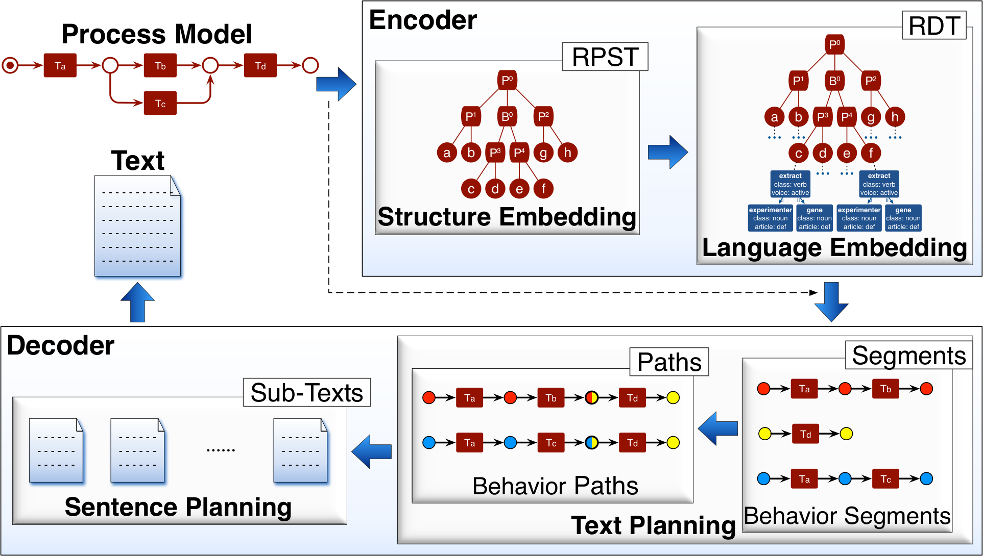
To solve these challenges (C1-C6), we propose BePT which is built on the encoder-decoder framework inspired from machine translation systems (Schulz et al. 2018; Cho et al. 2014b; Cho et al. 2014a). The encoder creates an intermediate tree representation from the original model and the decoder generates its NL descriptions. Figure 3 presents a high-level framework of BePT, including four main phases: Structure Embedding, Language Embedding, Text Planning and Sentence Planning (Leopold et al. 2012a; Leopold et al. 2014; Qian et al. 2017):

Refer to caption — Figure 3. High-level view of BePT’s framework.

1)

Structure Embedding (C1): Embedding the structure information of the original model into the intermediate representation.
2)

Language Embedding (C2): Embedding the language information of the original model into the intermediate representation.
3)

Text Planning (C3, C4): Linearizing the non-linear tree representation into linear representations.
4)

Sentence Planning (C5, C6): Generating NL text by employing pre-defined language templates and NL tools.

4.1. Structure Embedding

We take a simplified model $N_{*}$ , shown in Figure 4, as our running example due to its complexity and representativeness. A complex sub-component (any structure is possible) in the original model is replaced by the black single activity $T_{e}$ . The simplified model $N_{*}$ is also complex since it contains a main path and two loops.

We employ a simplification algorithm from (Qian et al. 2017) to replace each sub-model with a single activity to obtain a simplified but behavior-equivalent one because a model containing many sub-models may complicate the behavior extraction (Qian et al. 2017). In the meantime, the simplification operation causes no information loss (Qian et al. 2017) since the simplified part will be visited in the deeper recursion. We emphasize that this simplification step is easy and extremely necessary for behavior correctness (see Appendix A for proof of behavior correctness).

Next, we analyze its structural skeleton and then create the RPST of $N_{*}$ . Finally, we embed its structural information - RPST - into a tree representation (as shown in the upper part of Figure 5).

Figure 4. A simplified model (

N_{*}

). The original complex component (any structure is possible) is simplified by the black element (a single activity).

4.2. Language Embedding

4.2.1. Extract Linguistic Information

This step sets out to recognize NL labels and extract the main linguistic information (Leopold et al. 2011; Leopold et al. 2012b; Leopold 2013). For each NL label, we first examine prepositions and conjunctions. If prepositions or conjunctions are found, respective flags are set to true. Then we check if the label starts with a gerund. If the first word of the label has an “ing” suffix, it is verified as a gerund verb phrase (e.g., “extracting gene”). Next, WordNet (Miller 1995) is used to learn if the first word is a verb. If so, the algorithm refers it to a verb phrase style (e.g., “extract gene”). In the opposite case, the algorithm proceeds to check prepositions in the label. A label containing prepositions the first of which is “of” is qualified as a noun phrase with of prepositional phrase (e.g., “creation of database”). If the label is categorized to none of the enumerated styles, the algorithm refers it to a noun phrase style (e.g., “gene extraction”). Finally, we similarly categorize each activity label into four labeling styles (gerund verb phrase, verb phrase, noun phrase, noun phrase with of prepositional phrase).

Lastly, we extract the linguistic information - role, action and objects - depending on which pattern it triggers. For example, in $N_{*}$ , the label of $T_{d}$ triggers a verb phrase style. Accordingly, the action lemma “remove” and the noun lemma “impurity” are extracted.

4.2.2. Create DSynTs

Once this main linguistic information is extracted, we create a DSynT for each label by assigning the main verb and main nouns including other associated meta information (Ballesteros et al. 2014; Lavoie and Rambow 1997) (as shown in the lower part of Figure 5).

For better representation, we concatenate each DSynT root node to its corresponding RPST leaf node, and we call this concatenated tree RPST-DSynTs (RDT). The RDT of $N_{*}$ is shown in Figure 5.

Figure 5. The RDT of

N_{*}

. Some parts are replaced by the ellipsis due to the limited space.

So thus far, we have embedded the structural information (RPST) and the linguistic information (DSynTs) of the original process model into the intermediate representation RDT. Then, it is passed to the decoder phase.

4.3. Text planning

The biggest gap between a model and a text is that a model contains sequential and concurrent semantics (Goltz and Reisig 1983), while a text only contains sequential sentences. Thus, this step focuses on transforming a non-linear model into its linear representations.

In order to maintain behavior correctness, we first create the CFP of the original model because a CFP is a complete and minimal behavior-unfolded graph of the original model (McMillan and Probst 1995; Esparza et al. 2002; Engelfriet 1991). Figure 6 shows the CFP of $N_{*}$ . According to Definition 3.6, $T_{d1}$ and $T_{e1}$ are two cut-off transitions, thus, no transitions follow them.

Besides, we introduce a basic concept: shadow place. Shadow places ( $\mathcal{SP}$ ) are those CFP places that are: 1) mutual with CFP boundary places or 2) mapped to the boundary places of the original model.

Example 0.

In Figure 6, the five colored places are shadow places of $\mathbb{N}_{*}$ ( $P_{a1},P_{b1},P_{a2},P_{d1},P_{b2}\in\mathcal{SP}(\mathbb{N}_{*})$ ). Note that theyare mutual with the CFP boundary places, and $P_{d1}$ is mapped to the boundary places of the original model $N_{*}$ ( $\hbar(P_{d1})=P_{d}$ ). Intuitively, a shadow place represents the repetition of a boundary place in the original model or its CFP.

Figure 6. The CFP of

N_{*}

(

\mathbb{N}_{*}

). The five colored places are shadow places. A shadow place is shown in same (different) color as its mutual (non-mutual) places.

4.3.1. Behavior Segment

Since we have obtained the behavior-unfolded graph, i.e., CFP, now, we define (behavior) segments which capture the minimal behavioral characteristics of a CFP to avoid state space explosion problem.

Definition 0 (Behavior Segment).

Given a net $N=(P,T,F)$ and its CFP $\mathbb{N}$ , a behavior segment $\mathbb{S}=(P^{\prime},T^{\prime},F^{\prime})$ is a connected sub-model of $\mathbb{N}$ satisfying:

1)

$\bullet\mathbb{S}\bullet\subseteq\mathcal{SP}(\mathbb{N})\wedge P^{\prime}\backslash\bullet\mathbb{S}\bullet\cap\mathcal{SP}(\mathbb{N})=\varnothing$ , i.e., all boundary nodes are shadow places and all other places are not.
2)

If each place in $\hbar(\bullet\mathbb{S})$ contains one token, after firing all transitions in $\hbar(T^{\prime})$ , each place in $\hbar(\mathbb{S}\bullet)$ contains just one token while other places in $\hbar(\mathbb{N})$ are empty.

Example 0.

According to Definition 4.2, if we put $\hbar(P_{a1})=P_{a}$ (in $N_{*}$ ) a token, $T_{a}$ (in $N_{*}$ ) can be fired, and after this firing, only $P_{b}$ (in $N_{*}$ ) contains a token. Therefore, the sub-model containing nodes $P_{a1},T_{a1},P_{b1}$ (in $\mathbb{N}_{*}$ ) and their adjacency arcs is a behavior segment. All behavior segments of $\mathbb{N}_{*}$ are shown in Figure 8(a) (careful readers might have realized that these four segments belong to sequential structures, i.e., all segments contain only SESE nodes. However, a behavior segment can be a non-sequential structure, i.e., containing multiple-incoming or multiple-outgoing nodes. For example, the behavior segment of a transition-bounded model is homogeneous to itself, containing four multiple-incoming or multiple-outgoing nodes).

4.3.2. Linking Rule

Behavior segments capture the minimal behavioral characteristics of a CFP. In order to portray the complete characteristics, we link these segments to obtain all possible behavior paths by applying the linking rule below.

Definition 0 (Linking Rule).

For two segments $\mathbb{S}_{i}=(P_{i},T_{i},F_{i})$ and $\mathbb{S}_{j}=(P_{j},T_{j},F_{j})$ , if $\hbar(\mathbb{S}_{i}\bullet)\supseteq\hbar(\bullet\mathbb{S}_{j})$ we say they are linkable. If two places $p_{i}\in\mathbb{S}_{i}\bullet,p_{j}\in\bullet\mathbb{S}_{j}$ are mutual, we say $p_{i}$ is the joint place of $p_{j}$ denoted as $\mathcal{J}(p_{j})=p_{i}$ where $\mathcal{J}$ is the joint function. If $n\notin\bullet\mathbb{S}_{j}$ , $\mathcal{J}(n)=n$ . The linked segment of two linkable segments $\wr\mathbb{S}_{i},\mathbb{S}_{j}\wr=(P\wr,T\wr,F\wr)$ satisfies:

1)

$P\wr=P_{i}\cup(P_{j}\backslash\bullet\mathbb{S}_{j})$ , i.e., the places of a linked segment consist of all places in $\mathbb{S}_{i}$ and all non-entry places in $\mathbb{S}_{j}$ .
2)

$T\wr=T_{i}\cup T_{j}$ , i.e., the transitions of a linked segment consist of all transitions in $\mathbb{S}_{i}$ and $\mathbb{S}_{j}$ .
3)

$F\wr=\{\langle\mathcal{J}(u),\mathcal{J}(v)\rangle|\langle u,v\rangle\in F_{i}\cup F_{j}\}$ , i.e., the arcs of a linked segment are the $\mathcal{J}$ -replaced arcs of $\mathbb{S}_{i}$ and $\mathbb{S}_{j}$ .

Similarly, $\wr\mathbb{S}_{1},\mathbb{S}_{2},\cdots,\mathbb{S}_{n}\wr$ denotes the recursive linking of two segments $\wr\mathbb{S}_{1},\mathbb{S}_{2},\cdots,\mathbb{S}_{n-1}\wr$ and $\mathbb{S}_{n}$ . The graphical explanation of the linking rule is shown in Figure 7.

Figure 7. The graphical explanation of linking two segments

\mathbb{S}_{i},\mathbb{S}_{j}

. The joint nodes are shown in red/blue color.

(a) The behavior segments of

\mathbb{N}_{*}

(b) The partial behavior paths of

\mathbb{N}_{*}

Figure 8. The behavior segments and the partial behavior paths of

\mathbb{N}_{*}

4.3.3. Behavior Path

According to the linking rule, we can obtain all linked segments. However, a linked segment might involve infinite linking due to concurrent and loop behaviors (Goltz and Reisig 1983). Hence, we apply truncation conditions to avoid infinite linking, which leads to the definition of a (behavior) path. Behavior paths capture complete behavioral characteristics of a CFP.

Definition 0 (Behavior Path).

A segment $\mathbb{P}=\wr\mathbb{S}_{1},\mathbb{S}_{2},\cdots,\mathbb{S}_{n}\wr$ of $\mathbb{N}$ is a behavior path iff one of the following conditions holds:

1)

$\bullet\mathbb{P}=\bullet\mathbb{N}\wedge\mathbb{P}\bullet\subseteq\mathbb{N}\bullet$ , i.e., $\mathbb{P}$ starts from the entry of $\mathbb{N}$ and ends at one of the exits of $\mathbb{N}$ .
2)

$\hbar(\bullet\mathbb{P})=\hbar(\mathbb{P}\bullet)$ , i.e., $\mathbb{P}$ starts from a shadow node (set) and ends at this node (set), i.e., loop structure.

Example 0.

Take Figure 8(a) as an example. Since $\hbar(\mathbb{S}_{3}\bullet)=\hbar(\{P_{a2}\})$
= $\{P_{a}\}\supseteq\hbar(\bullet\mathbb{S}_{1})=\hbar(\{P_{a1}\})=\{P_{a}\}$ , it follows that $\mathbb{S}_{3}$ and $\mathbb{S}_{1}$ are linkable with $\mathcal{J}(p_{a1})=p_{a2}$ , and $\hbar(\bullet\wr\mathbb{S}_{3},\mathbb{S}_{1}\wr)=\hbar(\wr\mathbb{S}_{3},\mathbb{S}_{1}\wr\bullet)=\{P_{b}\}$ . Thus, the linked segment $\wr\mathbb{S}_{3},\mathbb{S}_{1}\wr$ is a behavior path ( $\mathbb{P}_{4}$ in Figure 8(b)). Partial behavior paths of $N_{*}$ are shown in Figure 8(b).

4.4. Sentence planning

After extracting all behavior paths from a process model. Then, each path is recognized as a polygon component and then put into BePT (a recursive algorithm). The endpoint is a non-decomposable trivial component, i.e., node. When encountering a gateway node (split or join node), the corresponding DSynT (a pre-defined language template) is retrieved from RDT or pre-defined XML-format files. When encountering a SESE node, the corresponding DSynT is extracted from the embedded RDT. After obtaining all DSynTs, the sentence planning phase is triggered.

Sentence planning sets out to generate a sentence for each node. The main idea here is to utilize a DSynT to create a NL sentence (Lavoie and Rambow 1997; Ballesteros et al. 2014; Leopold et al. 2014). The generation task is divided into two levels: template sentence and activity sentence generation.

$\bullet$

Template sentences focus on describing the behavioral information related to the non-terminal RPST nodes. We provide 32 language template DSynTs (including split, join, dead transition, deadlock (van der Aalst et al. 2004) etc,) to represent corresponding semantic(s). The choice of a template depends on three parameters (Leopold et al. 2012a; Leopold et al. 2014; Qian et al. 2017): 1) the existence of a gateway label; 2) the gateway type; 3) the number of outgoing arcs. For instance, for a place with multiple outgoing arcs, the corresponding template sentence “One of the branches is executed” will be retrieved.
$\bullet$

Activity sentences focus on describing a single activity related to the terminal (leaf) RPST nodes. RDT representation has embedded all DSynT messages; thus, for each activity, we can directly access its DSynT from RDT.

After preparing all DSynTs in the text planning phase, we employ three steps to optimize the expression before the final generation:

1)

Checking whether each DSynT lacks necessary grammar meta-information to guarantee its grammatical correctness.
2)

Pruning redundant TARs to ensure that the selected TARs will not be repeated (Pruning Rule). For example, $T_{a}\prec T_{b}$ derived by $\mathbb{P}_{2}$ or $\mathbb{P}_{4}$ in Figure 8(b) is a redundant TAR because it has been concluded in $\mathbb{P}_{1}$ .
3)

Refining the DSynT messages containing the same linguistic component between two consecutive sentences and making use of three aggregation strategies: role aggregation, action aggregation and object aggregation (Leopold et al. 2014; Qian et al. 2017).

After expression optimization, we employ the DSynT-based realizer RealPro (Lavoie and Rambow 1997) to realize sentence generation. RealPro requires a DSynT as input and outputs a grammatically correct sentence (Ballesteros et al. 2014). In a loop, every DSynT is passed to the realizer. The resulting NL sentence is then added to the final output text. After all sentences have been generated, the final text is presented to the end user.

Example 0.

The generated text of $N_{*}$ in Figure 4 is as follows (other state-of-the-art methods cannot handle this model):

\bullet

The following main branches are executed: 2)

\bullet

The experimenter extracts the genes. Then, he sequences the DNA. Subsequently, the experimenter records the data. 3)

\bullet

Attention, there are two loops which may conditionally occur: 4)

\bullet

After sequencing DNA, the experimenter can also remove impurities if it is not clean. Then, he continues extracting genes. 5)

\bullet

After recording the data, there is a series of activities that need to be finished before DNA sequencing: 6)

\bullet

***

Template sentences (1, 3, 7) describe where the process starts, splits, joins and ends. Activity sentences (2, 4, 5) describe each sorted behavior path. The paragraph placeholder (6) can be flexibly replaced according to the sub-text of the simplified component $T_{e}$ . We can see that BePT first describes the main path (“ $T_{a}$ $\rightarrow$ $T_{b}$ $\rightarrow$ $T_{c}$ ”) before two possible loops (“ $T_{a}$ $\rightarrow$ $T_{b}$ $\rightarrow$ $T_{d}$ ”, “ $T_{c}$ $\rightarrow$ $T_{e}$ $\rightarrow$ $T_{b}$ ”). These three paragraphs of the generated text correspond to three correct firing sequences of the original model, the generated text contains just enough descriptions to reproduce the original model without redundant descriptions.

Table 1. Statistics of the evaluation datasets. N=Total number of models per source; SMR=The ratio of structured models to all models; min=The minimum value per source; ave=The average value per source; max=The maximum value per source.

Source	Type	N	SMR $\downarrow$	Place			Transition			Arc			RPST depth
Source	Type	N	SMR $\downarrow$	min	ave	max	min	ave	max	min	ave	max	min	ave	max
SAP	Industry	72	100.00%	2	3.95	13	1	3.12	12	2	6.75	24	1	1.85	5
DG	Industry	38	94.74%	3	7.65	22	2	7.85	17	4	16.02	44	1	2.55	7
TC	Industry	49	81.63%	6	10.10	17	6	10.62	19	14	21.87	38	1	3.92	7
SPM	Academic	14	57.00%	2	7.28	12	1	7.40	15	2	15.49	30	1	2.93	5
IBM	Industry	142	53.00%	4	39.00	217	3	26.46	145	6	79.84	456	1	5.21	12
GPM	Academic	36	42.00%	4	11.15	19	3	11.55	24	6	24.92	48	1	3.22	5
BAI	Academic	38	28.95%	4	10.54	21	2	9.93	24	6	22.92	49	1	3.24	5

4.5. Property Analysis

We emphasize BePT’s three strong properties - correctness, completeness and minimality. Specifically, given a net system $S=(N,M)$ and its TAR set $\mathcal{T}(S)$ . The behavior path set $\mathcal{P}$ of $\mathbb{N}$ by the linking rule (Definition 4.4) satisfies: 1) behavior correctness, $\forall\mathbb{P}\in\mathcal{P}\Rightarrow\mathcal{T}(\mathbb{P})\subseteq\mathcal{T}(S)$ ; 2) behavior completeness, $\forall\tau\in\mathcal{T}(S)\Rightarrow\exists\mathbb{P}\in\mathcal{P},\tau\in\mathcal{T}(\mathbb{P})$ ; 3) description minimality, each TAR $\mathcal{T}(S)$ by the pruning rule is described only once in the final text. Please see Appendices A, B and C for detailed proofs.

5. Evaluation

We have conducted extensive qualitative and quantitative experiments. In this section, we report the experimental results to answer the following research questions:

RQ1

Capability: Can BePT handle more complex model patterns than existing techniques?
RQ2

Detailedness: How much information does BePT express?
RQ3

Consistency: Is BePT text consistent to the original model?
RQ4

Understandability: Is BePT text easy to understand?
RQ5

Reproducibility: Can the original model be reproduced only from its generated text?

5.1. Experimental Setup

In this part, we describe our experimental datasets, the baselines and the experiment settings.

5.1.1. Datasets

We collected and tested on seven publicly accessible datasets: SAP, DG, TC, SPM, IBM, GPM, BAI (Leopold et al. 2012a; Leopold et al. 2014; Qian et al. 2017; Qian and Wen 2018). Among them, SAP, DG, TC, IBM are from industry (enterprises etc,) and SPM, GPM, BAI are from academic areas (literature, online tutorials, books etc,). The characteristics of the seven datasets are summarized in Table 1 (sorted by the decreasing ratio of structured models $\bm{SMR}$ ). There are a total of 389 process models consisting of real-life enterprise models (87.15%) and synthetic models (12.85%). The number of transitions varies from 1 to 145 and the depth of RPSTs varies from 1 to 12. The statistical data is fully skewed due to the different areas, amounts and model structures.

5.1.2. Baseline Methods

We compared our proposed process translator BePT with the following three state-of-the-art methods:

$\bullet$

Leo (Leopold et al. 2012a). It is the first structure-based method focusing mainly on structured components: trivial, bond and polygon.
$\bullet$

Hen (Leopold et al. 2014). It is the extended version of Leo focusing mainly on rigid components with longest-first strategy.
$\bullet$

Goun (Qian et al. 2017). It is a state-of-the-art structured-based method focusing mainly on unfolding model structure without considering its behaviors.

5.1.3. Parameter Settings

We implemented BePT based on jBPT²² 2 https://code.google.com/archive/p/jbpt/. An easy-to-use version of BePT is also publicly available³³ 3 https://github.com/qianc62/BePT. We include an editable parameter for defining the size of a paragraph and predefine this parameter with a value of 75 words. Once this threshold is reached, we use a change of the performing role or an intermediate activity as an indicator and respectively introduce a new paragraph. Besides, we use the default language grammar style of subject-predicate-object and object-be-predicated-by-subject to express a sentence (Leopold et al. 2012a; Leopold et al. 2014; Qian et al. 2017). Finally, we set all parameters to valid for all methods, i.e., to generate intact textual descriptions without any reduction.

5.2. Results

5.2.1. Capability (RQ1)

As discussed earlier, a rigid is a region that captures an arbitrary model structure. Thus, these seven datasets are representative enough as the $SMR$ varies from 100% (structured models) to 28.95% (unstructured complex models). We analyzed and compared all process models. Table 2 reports their handling capabilities w.r.t some representative complex patterns (Qian et al. 2017; Liu and Kumar 2005).

Table 2. The handling capabilities of four P2T methods w.r.t. some representative patterns.

Type	Pattern	Leo	Hen	Goun	BePT
T, B, P	Trivial	✓	✓	✓	✓
	Polygon	✓	✓	✓	✓
	Easy Bond	✓	✓	✓	✓
	Easy Loop	✓	✓	✓	✓
	Unsymmetrical Bond				✓
R	Place Rigid		✓	✓	✓
	Transition Rigid				✓
	Mix Rigid				✓
	Intersectant Loop				✓
	Non-free-choice Construct			✓	✓
	Invisible or Duplicated Task			✓	✓
	Multi-layered Embedded			✓	✓
Extra	Modeling Information				✓
Extra	Multi-layered Paragraph			✓	✓
Total		4	5	9	14

First, we can see that BePT shows the best handling capabilities. Among the 14 patterns, BePT can handle them all, which is better than Goun that can handle 9 patterns. Second, all four methods can handle structured models well, while Goun and BePT can handle unstructured models, and BePT can even further provide extra helpful messages. Third, the R and the Extra parts show that BePT can handle rigids of arbitrary complexity even if the model is unsymmetrical, non-free-choice or multi-layered. From these results, we can conclude that the behavior-based method BePT is sufficiently powerful to address complex structures.

5.2.2. Detailedness (RQ2)

In the sentence planning phase, BePT checks the grammatical correctness of each DSynT so that the generated text can accord with correct English grammar. Here, instead of comparing the grammatical correctness, we summarize the structural characteristics of all generated texts in Table 3.

Table 3. Average number of words and sentences per text. Red numbers denote the maximum and green numbers denote the minimum per dataset.

	Words/Text				Sentences/Text
	Leo	Hen	Goun	BePT	Leo	Hen	Goun	BePT
SAP	38.0	38.0	38.1	38.1	6.0	6.0	6.2	6.2
DG	74.0	79.7	79.6	85.3	13.0	15.0	15.0	15.7
TC	99.2	110.8	112.4	135.0	12.2	15.5	15.7	18.7
SPM	41.5	54.1	55.6	100.9	5.8	7.9	8.1	14.1
IBM	140.2	180.7	182.9	191.9	74.2	80.7	81.7	86.2
GPM	38.3	50.8	53.8	147.0	6.2	7.5	7.9	16.2
BAI	25.7	31.7	32.6	111.3	2.7	4.4	4.6	15.7
Total	66.7	78.0	79.3	115.3	17.2	19.6	19.9	22.3

A general observation is that BePT texts are longer than the other texts. Leo, Hen, and Goun texts contain an average of 66.7, 78.0 and 79.3 word length and 17.2, 19.6, 19.9 sentence length respectively, while BePT texts include an average of 115.3 words and 22.3 sentences. However, this does not imply that BePT texts are verbose, using longer sentences to describe the same content. Rather, Leo, Hen, Goun ignore some modeling-level messages related to soundness and safety (van der Aalst 2000; van der Aalst et al. 2004), but BePT supplements them. Therefore, we conclude that BePT generates more detailed messages to provide additional useful information. Of course, while all parameters are set to be valid in this experiment, BePT is actually configurable, i.e., users can set parameters to determine whether to generate these complementary details or not.

5.2.3. Consistency (RQ3)

A generally held belief is that the hierarchical organization of texts will hugely influence readability since paragraph indentation can reflect the number of components, the modeling depth of each activity, etc. Considering the generated text of the running example (Example 4.7), if the text contains no paragraph indentation, i.e., each paragraph starts from the bullet point " $\bullet$ ", it will be much harder to fully reproduce the model semantics (Leopold et al. 2014; Qian et al. 2017).

In this part, we consider the detection of structural consistency between a process model and its corresponding textual descriptions. This task requires an alignment of a model and a text, i.e., activities in the texts need to be related to model elements and vice versa (de Leoni et al. 2015; Weidlich et al. 2011). For an activity $T$ , its modeling depth $md(T)$ is the RPST depth of $T$ , and its description depth $dd(T)$ is how deep it is indented in the text. For the activity set of a model, the modeling depth distribution is denoted as $\mathcal{X}=[md(T_{1}),md(T_{2}),...,md(T_{n})]$ and the description depth distribution is denoted as $\mathcal{Y}=[dd(T_{1}),dd(T_{2}),...,dd(T_{n})]$ . We employ a correlation coefficient to evaluate the consistency between the two distributions of $\mathcal{X}$ and $\mathcal{Y}$ as follows:

(1)

\rho(\mathcal{X},\mathcal{Y})=\frac{E[(\mathcal{X}-E\mathcal{X})(\mathcal{Y}-E\mathcal{Y})]}{\sqrt{D\mathcal{X}\cdot D\mathcal{Y}}}\in[-1.0,1.0]

where $E$ is the expectation function and $D$ is the variance function. The value of the $\rho(\mathcal{X},\mathcal{Y})$ function ranges from -1.0 (negatively related) to 1.0 (positively related).

Figure 9. The consistency distribution. The red color denotes the positive coefficient while the blue color denotes the negative coefficient.

Figure 9 shows the consistency results of the four P2T methods. First, BePT obtains the highest consistency value in every dataset, meaning that BePT positively follows the depth distribution of original models to the maximum extent. Notice that all methods obtain 1.00 consistency on the SAP dataset since all SAP models are structured. However, on the SPM dataset, BePT achieves 0.86 consistency, while the other methods are only at around 0.25. The main reason is that SPM contains plenty of close-to-structured rigids, which directly reflects the other methods’ drawbacks. Second, with lower $SMR$ , the consistency performance rapidly decreases. The most obvious updates occur in GPM and BAI where Leo, Hen and Goun even produce negative coefficient values, which demonstrates that they negatively relate the distribution of the original models even causing the opposite distribution, while BePT obtains 0.42 and 0.25 which shows that BePT is still positively related even while facing unstructured situations. Hence, we conclude that BePT texts conform better to the original models.

5.2.4. Understandability (RQ4)

In this section, we discuss the perplexity that reflects the textual understandability. It quantifies “how hard to understand” a model-text pair. This information entropy-based metric (Jianhua 1991) is inspired from the natural language processing techniques (Roark et al. 2007).

Consider a model-text pair $\langle\mathcal{M},\mathcal{T}\rangle$ in which the text $\mathcal{T}$ consists of a sequence of paragraphs $\langle S_{1},S_{2},\cdots,S_{n}\rangle$ . $\psi(S_{i})$ denotes the information gain of paragraph $S_{i}$ :

(2)

\psi(S_{i})=e^{|T^{\prime}|log_{2}|T^{\prime}|}\cdot|T^{\prime}|\cdot|U^{\prime}|

where $T^{\prime}$ is the described activity set and $U^{\prime}$ is the neglected activity set. This formula employs information entropy $|T^{\prime}|log_{2}|T^{\prime}|$ to describe the confusion of all activities in a paragraph. Its exponent value has the same magnitude of $|T^{\prime}|$ . We notice that if any activity cannot be generated in the text, the text system should reduce the understandability value with the original model, i.e., improve the perplexity of the text system; hence, it multiplies by $|U^{\prime}|$ .

When describing a single paragraph $S_{1}$ , the information gain (Han et al. 2012) of the text system is $\psi(S_{1})$ . After describing paragraph $S_{2}$ , the information gain changes to $\psi(S_{1})+\psi(S_{2})$ . Similarly, after describing all paragraphs, the information gain is $\Sigma_{i=1}^{n}\psi(S_{i})$ . These values are mapped to $n$ points $(i,\Sigma_{k=1}^{i}\psi(S_{k}))_{i=1}^{n}$ shown in Figure 10(a). We call the broken line linking all points the information gain line $IGL(\langle\mathcal{M},\mathcal{T}\rangle,S)$ . Then, we can define the perplexity of the text system $\mathcal{T}$ (the integral over all sentence perplexities):

(3)

perplexty(\langle\mathcal{M},\mathcal{T}\rangle)=\int_{0}^{n}IGL(\langle\mathcal{M},\mathcal{T}\rangle,s)ds,s\in\mathbb{R}

$IGL(S)$ intuitively measures whether the model-text pair system is understandable where a lower perplexity implies a higher understandability. We calculated this metric for each dataset and reported the results.

Figure 10(b) shows the perplexity results. We can see that BePT achieves the lowest perplexity in all datasets, i.e., best understandability. On average, the perplexity has been reduced from $10^{2.74}$ to $10^{0.98}$ . This results also show that the perplexity trend is Leo $\geq$ Hen $\geq$ Goun $\geq$ BePT, i.e., the understandability trend is Leo $\leq$ Hen $\leq$ Goun $\leq$ BePT.

5.2.5. Reproducibility (RQ5)

This part evaluates the reproducibility of the generated text, i.e., could the original model be reproduced from the generated text?

For each model-text pair ( $\mathcal{M},\mathcal{T}$ ), we manually back-translate (extract) the process model from the generated text and compare the elements between the original and the extracted models. All back-translators are provided only the generated texts without them knowing any information of the original models. They reproduce the original models from the texts according to their own understanding. After translation, we evaluate the structural and behavioral reproducibility between the original model and the extracted one. If an isomorphic model $\mathcal{M}$ can be reproduced, we can believe that the text $\mathcal{T}$ contains enough information to reproduce the original model, i.e., excellent reproducibility. We evaluate the P2T performance using the $F_{1}$ measure (the harmonic average of recall and precision) which is inspired by the data mining field (Han et al. 2012):

(4)

F_{1}=\frac{(1+\beta^{2})\cdot precision\cdot recall}{\beta^{2}\cdot precision+recall}\in[0.0,1.0]

where $\beta$ is the balance weight. In our experiments, equal weights ( $\beta=1.0$ ) are assigned to balance recall and precision. The higher the $F_{1}$ is, the better the reproducibility is.

Structural Reproducibility. Figure 11 shows the results of four dimensions (place, transition, gateway, element). First, we can see that the $F_{1}$ value of the four methods falls from 100% to a lower value w.r.t. decreasing $SMR$ . For GPM and BAI datasets, Leo achieves only around 40%. The low-value cases significantly affect the ability to understand or reproduce the original model, and it reflects the general risk that humans may miss elements when describing a model, i.e., they lose around 60% information. Still, Hen achieves around 90% while BePT hits 100%, i.e., Goun and BePT lose least information. We can conclude that, among the four P2T methods, BePT achieves the highest reproducibility, followed by Goun and then Hen. The structural reproducibility performance also shows the trend, Leo $\leq$ Hen $\leq$ Goun $\leq$ BePT.

Behavioral Reproducibility. Behavioral reproducibility aims to evaluate the extent of correctly expressed behavior, i.e., how many correct behaviors are expressed in the generated texts. We also use $F_{1}$ to evaluate behavioral performance. In this part, we use TAR (local) and trace (global) to reflect the model behaviors. As trace behaviors exist space explosion problem, thus, for trace F-measure, we only evaluate these models without loop behavior.

Figure 12 shows the results for the behavior dimensions (TAR, trace). The results show that BePT outperforms Leo, Hen and Goun significantly in terms of both TAR and trace performance. Leo performance falls sharply with decreasing $SMR$ , while Hen and Goun drop more gently than Leo and they achieve around 70% on BAI for trace $F_{1}$ . BePT gets the highest $F_{1}$ of around 100% for both TAR and trace measures, and BePT also produces a distinct improvement on TAR and trace $F_{1}$ over other methods. From these two performance results, we can conclude that BePT showcases the best reproducibility over the state-of-the-art P2T methods.

6. Conclusion and Future Work

We present a behavior-based process translator. It first combines the structural and linguistic information into an RDT tree before decoding it by extracting the behavior paths. Then, we use NL tools to generate textual descriptions. Our experiments show the significant improvements that result on capability, detailedness, consistency, understandability and reproducibility. This approach can unlock the hidden value that lies in large process repositories in the cloud, and make them more reusable.

We also list some potential limitations of this study. Above all, when the model is unsound, BePT informs the user that the model contains non-sound or wrong parts but without giving any correction advice. Another drawback concerns manual extraction of the NL text because of the limited number of participants. We cannot guarantee that each extraction rule for a generated text is identical. Thus, generating the correction advice and automatic reverse translation would also be of interest in future studies.

Appendices

Appendix A The Proof of Behavior Correctness

Property 1.

Given a net system $S=(N,M)$ and its TAR set $\mathcal{T}(S)$ . The behavior path set $\mathcal{P}$ of its CFP $\mathbb{N}$ by the linking rule (Definition 4.4) satisfies behavior correctness, $\forall\mathbb{P}\in\mathcal{P}\Rightarrow\mathcal{T}(\mathbb{P})\subseteq\mathcal{T}(S)$ .

Proof 1.

Given two Petri nets $N_{i}=(P_{i},T_{i},F_{i}),N_{j}=(P_{j},T_{j},F_{j})$ , we assume $\mathbb{P}=\wr\mathbb{S}_{1},\mathbb{S}_{2},\cdots,\mathbb{S}_{n}\wr$ . Then, consider two situations: a) inside a single segment; b) between the linking of two segments:

a)

The initial (default) marking $\bullet S$ is also the the initial marking of $\hbar(\mathbb{S}_{1})$ , i.e., the marking $\bullet\mathbb{S}_{1}$ is reachable. According to the definition of behavior segment, $\mathbb{S}_{1}\bullet$ is reachable from $\bullet\mathbb{S}_{1}$ , and the firing rule guarantees $\mathcal{T}(\mathbb{S}_{1})\subseteq\mathcal{T}(S)$ . After executing $\mathbb{S}_{1}$ , $\bullet\mathbb{S}_{2}$ is reachable as $\mathbb{S}_{1}\bullet\supseteq\bullet\mathbb{S}_{2}$ , so that $\mathcal{T}(\mathbb{S}_{2})\subseteq\mathcal{T}(S)$ holds. Similarly, $\wr\mathbb{S}_{1},\mathbb{S}_{2},\cdots,\mathbb{S}_{i-1}\wr\bullet\supseteq\bullet\mathbb{S}_{i}\Rightarrow\mathcal{T}(\mathbb{S}_{i})\subseteq\mathcal{T}(S),i\in 1,2\cdots n$ holds.
b)

For two segments $\mathbb{S}_{i},\mathbb{S}_{i+1},i\in 1,2\cdots n-1$ , we use the notation $\mathcal{T}(\mathbb{S}_{i}\wr\mathbb{S}_{i+1})$ to denote the TAR set in the joint points, i.e., $\mathcal{T}(\mathbb{S}_{i}\wr\mathbb{S}_{i+1})=\{a\prec b|a\in\bullet(\mathbb{S}_{i}\bullet)\wedge b\in(\bullet\mathbb{S}_{i+1})\bullet\}$ . Since $\mathbb{S}_{i}\bullet\supseteq\bullet\mathbb{S}_{i+1}$ guarantees that $(\bullet\mathbb{S}_{i+1})\bullet$ can be fired after firing $\bullet(\mathbb{S}_{i}\bullet)$ , i.e., $\mathcal{T}(\mathbb{S}_{i}\wr\mathbb{S}_{i+1})\subseteq\mathcal{T}(S)$ . Therefore, $\mathcal{T}(\wr\mathbb{S}_{i},\mathbb{S}_{i+1}\wr)=\mathcal{T}(\mathbb{S}_{i})\cup\mathcal{T}(\mathbb{S}_{i+1})\cup\mathcal{T}(\mathbb{S}_{i}\wr\mathbb{S}_{i+1})\subseteq\mathcal{T}(S),i\in 1,2\cdots n-1$ .

According to the above two points, we can conclude that $\forall\mathbb{P}\in\mathcal{P}\Rightarrow\mathcal{T}(\mathbb{P})=\mathcal{T}(\mathbb{S}_{1},\mathbb{S}_{2},\cdots,\mathbb{S}_{n})=\mathcal{T}(\mathbb{S}_{1})\cup\mathcal{T}(\mathbb{S}_{2})\cup\cdots\cup\mathcal{T}(\mathbb{S}_{n})\cup\mathcal{T}(\mathbb{S}_{1}\wr\mathbb{S}_{2})\cup\mathcal{T}(\mathbb{S}_{2}\wr\mathbb{S}_{3})\cup\cdots\cup\mathcal{T}(\mathbb{S}_{n-1}\wr\mathbb{S}_{n})\subseteq\mathcal{T}(S)$ .

Appendix B The Proof of Behavior Completeness

Property 2.

Given a net system $S=(N,M)$ and its TAR set $\mathcal{T}(S)$ . The behavior path set $\mathcal{P}$ of its CFP $\mathbb{N}$ by linking rule (Definition 4.4) satisfies behavior completeness, $\forall\tau\in\mathcal{T}(S)\Rightarrow\exists\mathbb{P}\in\mathcal{P},\tau\in\mathcal{T}(\mathbb{P})$ .

Proof 2.

For any TAR $\tau=a\prec b\in\mathcal{T}(S)$ , the place set $a\bullet\cap\bullet b$ is denoted as $\mathscr{P}$ . The sub-model $(\mathscr{P},\{a,b\},\{a\}\times\mathscr{P}\cup\mathscr{P}\times\{b\})$ is denoted as $\mathscr{N}$ . We use $N_{i}\propto N_{j}$ to denote $P_{i}\subseteq P_{j}\wedge T_{i}\subseteq T_{j}\wedge F_{i}\subseteq F_{j}$ , i.e., $N_{i}$ is a sub-model of $N_{j}$ . Then, consider the following situations:

a)

When $\forall p\in\mathscr{P},p\notin\mathcal{SP}(\mathbb{N})$ , there is no $p\in\mathscr{P}$ that can be the boundary node of a segment according to Definition 4.2 ( $\mathcal{SP}$ -bounded). Hence, $\mathscr{N}$ can only exist in the middle of a segment, i.e., $\exists\mathbb{S}_{i},\mathbb{P}_{j}\Rightarrow\mathscr{N}\propto\mathbb{S}_{i}\propto\mathbb{P}_{j}\in\mathcal{P}\Rightarrow\tau\in\mathcal{T}(\mathscr{N})\subseteq\mathcal{T}(\mathbb{P}_{j})$ .
b)

When $\forall p\in\mathscr{P},p\in\mathcal{SP}(\mathbb{N})$ , $\mathscr{P}$ is split, being the sink set of a certain segment $\mathbb{S}_{i}$ and the source set of a certain segment $\mathbb{S}_{j}$ ( $\mathcal{SP}$ -bounded), i.e., $\mathscr{P}=\mathbb{S}_{i}\bullet=\bullet\mathbb{S}_{j}$ always holds. Hence, $\exists\mathbb{S}_{i},\mathbb{S}_{j},\mathbb{P}_{k}\Rightarrow\mathscr{N}\propto\wr\mathbb{S}_{i},\mathbb{S}_{j}\wr\propto\mathbb{P}_{k}\in\mathcal{P}\Rightarrow\tau\in\mathcal{T}(\mathscr{N})\subseteq\mathcal{T}(\mathbb{P}_{k})$ .
c)

When $\exists p_{1},p_{2}\in\mathscr{P},p_{1}\notin\mathcal{SP}(\mathbb{N}),p_{2}\in\mathcal{SP}(\mathbb{N})$ , there is no $p\in\mathscr{P}$ can be the boundary node of a segment, or it contradicts Definition 4.2 (reply-hold). Hence, $\mathscr{N}$ can only exist in the middle of a segment, i.e., $\exists\mathbb{S}_{i},\mathbb{P}_{j}\Rightarrow\mathscr{N}\propto\mathbb{S}_{i}\propto\mathbb{P}_{j}\in\mathcal{P}\Rightarrow\tau\in\mathcal{T}(\mathscr{N})\subseteq\mathcal{T}(\mathbb{P}_{j})$ .
d)

When $\mathscr{P}=\varnothing$ , i.e., $a$ and $b$ are in a concurrent relation. There always exists a concurrent split transition $t$ . According to Definition 4.2, $\exists\mathbb{S}_{i}\Rightarrow t\in\mathbb{S}_{i}\wedge a,b\in\mathbb{S}_{i}$ (reply-hold). Thus, $\exists\mathbb{S}_{i},\mathbb{P}_{j}\Rightarrow\mathscr{N}\propto\mathbb{S}_{i}\propto\mathbb{P}_{j}\in\mathcal{P}\Rightarrow\tau\in\mathcal{T}(\mathscr{N})\subseteq\mathcal{T}(\mathbb{P}_{j})$ .

Appendix C The Proof of Description Minimality

Property 3.

For a net system $S=(N,M)$ , the pruned TARs $\mathcal{T}(S)$ by the Pruning Rule satisfies description minimality.

Proof 3.

According to Appendices B, for any TAR $\tau$ , it can always be derived from a certain behavior path, i.e., $\forall\tau\in\mathcal{T}(S)\Rightarrow\exists\mathbb{P}\in\mathcal{P},\tau\in\mathcal{T}(\mathbb{P})$ . Hence, for two TARs $\tau_{1},\tau_{2}$ of the original model with $\tau_{1}\in\mathcal{T}(\mathbb{P}_{i})\wedge\tau_{2}\in\mathcal{T}(\mathbb{P}_{j}),i<j$ . If $\tau_{1}\neq\tau_{2}$ , $\{\tau_{1},\tau_{2}\}\subseteq\mathcal{T}(S)$ always holds, while $\{\tau_{1}\}=\{\tau_{2}\}\subseteq\mathcal{T}(S)$ always holds if $\tau_{1}=\tau_{2}$ . Therefore, the pruning rule always keeps TARs appearing at the first time, i.e., $\mathcal{T}(S)$ satisfies behavior minimality.

Acknowledgements

The work was supported by the National Key Research and Development Program of China (No. 2016YFB1001101), the National Nature Science Foundation of China (No.71690231, No.61472207), and Tsinghua BNRist. We also would like to thank anonymous reviewers for their helpful comments.

References

(1)
Aysolmaz et al. (2018) Banu Aysolmaz, Henrik Leopold, Hajo A. Reijers, and Onur Demirörs. 2018. A Semi-automated Approach for Generating Natural Language Requirements Documents based on Business Process Models. Information and Software Technology 93 (2018), 14–29.
Ballesteros et al. (2014) Miguel Ballesteros, Bernd Bohnet, Simon Mille, and Leo Wanner. 2014. Deep-Syntactic Parsing. In Proceedings of COLING 2014, the 25th International Conference on Computational Linguistics: Technical Papers. Dublin City University and Association for Computational Linguistics, 1402–1413.
Boulakia and Leser (2011) Sarah Cohen Boulakia and Ulf Leser. 2011. Search, Adapt, and Reuse: The Future of Scientific Workflows. SIGMOD Record 40 (2011), 6–16.
Cho et al. (2014a) Kyunghyun Cho, Bart van Merrienboer, Dzmitry Bahdanau, and Yoshua Bengio. 2014a. On the Properties of Neural Machine Translation: Encoder-Decoder Approaches. In Proceedings of SSST-8, Eighth Workshop on Syntax, Semantics and Structure in Statistical Translation. Association for Computational Linguistics, 103–111.
Cho et al. (2014b) Kyunghyun Cho, Bart van Merrienboer, Caglar Gulcehre, Dzmitry Bahdanau, Fethi Bougares, Holger Schwenk, and Yoshua Bengio. 2014b. Learning Phrase Representations using RNN Encoder–Decoder for Statistical Machine Translation. In Proceedings of the 2014 Conference on Empirical Methods in Natural Language Processing (EMNLP). Association for Computational Linguistics, 1724–1734.
de Leoni et al. (2015) Massimiliano de Leoni, Fabrizio M. Maggi, and Wil M.P. van der Aalst. 2015. An Alignment-based Framework to Check the Conformance of Declarative Process Models and to Preprocess Event-log Data. Inf. Syst. 47, C (Jan. 2015), 258–277.
Engelfriet (1991) Joost Engelfriet. 1991. Branching Processes of Petri Nets. Acta Informatica 28, 6 (1991), 575–591.
Esparza et al. (2002) Javier Esparza, Stefan Römer, and Walter Vogler. 2002. An Improvement of McMillan’s Unfolding Algorithm. Formal Methods in System Design 20, 3 (2002), 285–310.
Gemino (2004) Andrew Gemino. 2004. Empirical Comparisons of Animation and Narration in Requirements Validation. Requirements Engineering 9, 3 (2004), 153–168.
Goble et al. (2010) Carole A Goble, Jiten Bhagat, Sergejs Aleksejevs, Don Cruickshank, Danius Michaelides, David Newman, Mark Borkum, Sean Bechhofer, Marco Roos, Peter Li, and David De Roure. 2010. myExperiment: A Repository and Social Network for the Sharing of Bioinformatics Workflows. Nucleic Acids Res 38, Web Server issue (Jul 2010), W677–82.
Goble and Roure (2007) Carole Anne Goble and David Charles De Roure. 2007. myExperiment: Social Networking for Workflow-using E-scientists. In WORKS@HPDC.
Goecks et al. (2010) Jeremy Goecks, Anton Nekrutenko, James Taylor, and The Galaxy Team. 2010. Galaxy: A Comprehensive Approach for Supporting Accessible, Reproducible, and Transparent Computational Research in the Life Sciences. Genome Biology 11, 8 (2010), R86.
Goltz and Reisig (1983) U. Goltz and W. Reisig. 1983. The Non-sequential Behaviour of Petri Nets. Information and Control 57, 2 (1983), 125–147.
Han et al. (2012) Jiawei Han, Micheline Kamber, and Jian Pei. 2012. Data Mining: Concepts and Techniques. Morgan Kaufmann, Boston, 327–391.
Hull et al. (2006) Duncan Hull, Katy Wolstencroft, Robert Stevens, Carole Goble, Mathew R Pocock, Peter Li, and Tom Oinn. 2006. Taverna: A Tool for Building and Running Workflows of Services. Nucleic Acids Research 34, Web Server issue (07 2006), W729–W732.
Jianhua (1991) Lin Jianhua. 1991. Divergence Measures based on the Shannon Entropy. IEEE Transactions on Information Theory 37, 1 (1991), 145–151.
Lavoie and Rambow (1997) Benoit Lavoie and Owen Rambow. 1997. A Fast and Portable Realizer for Text Generation Systems. In Proceedings of the Fifth Conference on Applied Natural Language Processing (ANLC ’97). Association for Computational Linguistics, Stroudsburg, PA, USA, 265–268.
Leopold (2013) Henrik Leopold. 2013. Parsing and Annotating Process Model Elements. In Natural Language in Business Process Models, Henrik Leopold (Ed.). Springer International Publishing, Cham, 49–80.
Leopold et al. (2012a) Henrik Leopold, Jan Mendling, and Artem Polyvyanyy. 2012a. Generating Natural Language Texts from Business Process Models. In Advanced Information Systems Engineering, Jolita Ralyté, Xavier Franch, Sjaak Brinkkemper, and Stanislaw Wrycza (Eds.). Springer Berlin Heidelberg, Berlin, Heidelberg, 64–79.
Leopold et al. (2014) Henrik Leopold, Jan Mendling, and Artem Polyvyanyy. 2014. Supporting Process Model Validation through Natural Language Generation. IEEE Transactions on Software Engineering 40, 8 (2014), 818–840.
Leopold et al. (2011) Henrik Leopold, Sergey Smirnov, and Jan Mendling. 2011. Recognising Activity Labeling Styles in Business Process Models. Enterprise Modelling and Information Systems Architectures 6 (2011), 16–29.
Leopold et al. (2012b) Henrik Leopold, Sergey Smirnov, and Jan Mendling. 2012b. On the Refactoring of Activity Labels in Business Process Models. Information Systems 37, 5 (2012), 443–459.
Li et al. (2015) Guang Li, Shubo Ma, and Yahong Han. 2015. Summarization-based Video Caption via Deep Neural Networks. In Proceedings of the 23rd ACM International Conference on Multimedia (MM ’15). ACM, New York, NY, USA, 1191–1194.
Liu and Kumar (2005) Rong Liu and Akhil Kumar. 2005. An Analysis and Taxonomy of Unstructured Workflows. In Business Process Management, Wil M. P. van der Aalst, Boualem Benatallah, Fabio Casati, and Francisco Curbera (Eds.). Springer Berlin Heidelberg, Berlin, Heidelberg, 268–284.
Malik and Bajwa (2013) Saleem Malik and Imran Sarwar Bajwa. 2013. Back to Origin: Transformation of Business Process Models to Business Rules. In Business Process Management Workshops, Marcello La Rosa and Pnina Soffer (Eds.). Springer Berlin Heidelberg, Berlin, Heidelberg, 611–622.
McMillan and Probst (1995) K. L. McMillan and D. K. Probst. 1995. A Technique of State Space Search based on Unfolding. Formal Methods in System Design 6, 1 (1995), 45–65.
Meziane et al. (2008) Farid Meziane, Nikos Athanasakis, and Sophia Ananiadou. 2008. Generating Natural Language specifications from UML class diagrams. Requirements Engineering 13, 1 (2008), 1–18.
Miller (1995) George A. Miller. 1995. WordNet: A Lexical Database for English. Commun. ACM 38, 11 (Nov. 1995), 39–41.
Murata (1989) T. Murata. 1989. Petri Nets: Properties, Analysis and Applications. Proc. IEEE 77, 4 (1989), 541–580.
Nielsen et al. (1979) Mogens Nielsen, Gordon Plotkin, and Glynn Winskel. 1979. Petri Nets, Event Structures and Domains. In Semantics of Concurrent Computation, Gilles Kahn (Ed.). Springer Berlin Heidelberg, Berlin, Heidelberg, 266–284.
Qian and Wen (2018) Chen Qian and Lijie Wen. 2018. Solving Algorithm for Scheduling Problem with Control-flow Constraints. Computer Integrated Manufacturing Systems 24, 7 (2018), 1598–1607.
Qian et al. (2017) Chen Qian, Lijie Wen, Jianmin Wang, Akhil Kumar, and Haoran Li. 2017. Structural Descriptions of Process Models Based on Goal-Oriented Unfolding. In Advanced Information Systems Engineering, Eric Dubois and Klaus Pohl (Eds.). Springer International Publishing, Cham, 397–412.
Roark et al. (2007) Brian Roark, Murat Saraclar, and Michael Collins. 2007. Discriminative N-gram Language Modeling. Comput. Speech Lang. 21, 2 (April 2007), 373–392.
Schulz et al. (2018) Philip Schulz, Wilker Aziz, and Trevor Cohn. 2018. A Stochastic Decoder for Neural Machine Translation. In Proceedings of the 56th Annual Meeting of the Association for Computational Linguistics (Volume 1: Long Papers). Association for Computational Linguistics, 1243–1252.
Starlinger et al. (2014) Johannes Starlinger, Bryan Brancotte, Sarah Cohen-Boulakia, and Ulf Leser. 2014. Similarity Search for Scientific Workflows. Proc. VLDB Endow. 7, 12 (Aug. 2014), 1143–1154.
van der Aalst et al. (2004) W. van der Aalst, T. Weijters, and L. Maruster. 2004. Workflow Mining: Discovering Process Models from Event Logs. IEEE Transactions on Knowledge and Data Engineering 16, 9 (2004), 1128–1142.
van der Aalst (1998) W. M. P. van der Aalst. 1998. Three Good Reasons for Using a Petri-Net-Based Workflow Management System. Springer US, Boston, MA, 161–182.
van der Aalst (2000) W. M. P. van der Aalst. 2000. Workflow Verification: Finding Control-Flow Errors Using Petri-Net-Based Techniques. Springer Berlin Heidelberg, Berlin, Heidelberg, 161–183.
Vanhatalo et al. (2008) Jussi Vanhatalo, Hagen Völzer, and Jana Koehler. 2008. The Refined Process Structure Tree. In Business Process Management, Marlon Dumas, Manfred Reichert, and Ming-Chien Shan (Eds.). Springer Berlin Heidelberg, Berlin, Heidelberg, 100–115.
Vinyals et al. (2015) Oriol Vinyals, Alexander Toshev, Samy Bengio, and Dumitru Erhan. 2015. Show and tell: A neural image caption generator. 2015 IEEE Conference on Computer Vision and Pattern Recognition (CVPR) (2015), 3156–3164.
Weidlich et al. (2011) M. Weidlich, J. Mendling, and M. Weske. 2011. Efficient Consistency Measurement Based on Behavioral Profiles of Process Models. IEEE Transactions on Software Engineering 37, 3 (2011), 410–429.
Wu et al. (2018) Huijun Wu, Chen Wang, Jie Yin, Kai Lu, and Liming Zhu. 2018. Sharing Deep Neural Network Models with Interpretation. In Proceedings of the 2018 World Wide Web Conference. 177–186.