Recovery of the fetal electrocardiogram for morphological analysis from two trans-abdominal channels via optimal shrinkage
Abstract.
We propose a novel algorithm to recover fetal electrocardiogram (ECG) for both the fetal heart rate analysis and morphological analysis of its waveform from two or three trans-abdominal maternal ECG channels. We design an algorithm based on the optimal-shrinkage under the wave-shape manifold model. For the fetal heart rate analysis, the algorithm is evaluated on publicly available database, 2013 PhyioNet/Computing in Cardiology Challenge, set A (CinC2013). For the morphological analysis, we analyze CinC2013 and another publicly available database, Non-Invasive Fetal ECG Arrhythmia Database (nifeadb), and propose to simulate semi-real databases by mixing the MIT-BIH Normal Sinus Rhythm Database and MITDB Arrhythmia Database. For the fetal R peak detection, the proposed algorithm outperforms all algorithms under comparison. For the morphological analysis, the algorithm provides an encouraging result in recovery of the fetal ECG waveform, including PR, QT and ST intervals, even when the fetus has arrhythmia, both in real and simulated databases. To the best of our knowledge, this is the first work focusing on recovering the fetal ECG for morphological analysis from two or three channels with an algorithm potentially applicable for continuous fetal electrocardiographic monitoring, which creates the potential for long term monitoring purpose.
Keywords: Fetal ECG morphology; noninvasive fetal ECG; optimal shrinkage; wave-shape manifold; nonlocal median
1. Introduction
Fetal cardiac arrhythmias are detected in at least 2% of pregnancies [1]. While many are transient, some sustained arrhythmias such as supraventricular tachycardia, ventricular tachycardia, and atrioventricular block may have significant consequences for the fetus and can result in fetal heart failure and demise. Therefore, detection and correct identification of fetal rhythm abnormalities is an important component of prenatal management [2]. Postnatal evaluation of the cardiac conduction system is performed by electrocardiography (ECG), with body-surface recording of cardiac electrical signal; however this is not possible in the fetus. The first observation of fetal electrocardiograph (fECG) was reported by Cremer in 1906 [3], when he accidentally recorded a small portion of the fetal tracing while assessing the ECG of a pregnant woman. However, over the ensuing years, multiple methods to obtain a refined non-invasive recording of the fetal ECG have been applied with some successes – some positive outcomes have been reported [4, 5, 6, 7, 8, 9] and there are devices that have obtained FDA clearance, e.g., the Monica AN24 monitor from Monica Healthcare (Nottingham, UK) and the MERIDIAN M110 monitor from MindChild Medical (North Andover, MA, USA) [10]. Fetal magnetocardiography has been developed, and successfully can provide morphology of the fetal ECG, including T wave morphology and QT interval [11, 12, 13]. However, the technique is quite expensive and is very limited in availability, leading to infrequent use. Given these difficulties, fetal echocardiography has been used a surrogate to the actual fECG. Through a combination of 2D imaging, M-mode imaging and Doppler analysis, correct identification of premature beats, tachyarrhythmia, and bradycardia such as heart block can be made and can guide medical management [14]. Despite the success of echocardiography, however, observation of the actual fECG signal would be very useful, especially for the diagnosis of conditions such as long QT syndrome, which may not result in obvious arrhythmias on echocardiography. Acquiring a morphologically refined fECG signal would assist in elucidating the origin and mechanisms of tachyarrhythmias and other conditions. Additionally, there has been some evidence that fetal ST analysis monitoring may help detect and alert fetal hypoxia, although this remains controversial [15].
In this paper, we focus on obtaining fECG from the ECG signal recorded from the mother’s abdomen, where the sensor is close to the fetus so that the fECG signal can be recorded [16, 17]. The signal is called trans-abdominal maternal ECG (ta-mECG). Importantly, the ta-mECG contains not only the fECG, but also the maternal cardiac activity, which we call the maternal abdominal ECG (mECG). Due to the existence of mECG, to obtain the fECG out of ta-mECG, we have to separate the fECG from the mECG. Since the fECG is often weaker than mECG, due to the inevitable noise, the fECG has a low signal-to-noise ratio (SNR). Moreover, due to the wide spectrum of ECG morphology and close heart rates of mother and fetus, the usual linear signal processing techniques do not work. All these facts make this biomedical signal processing challenging.
There have been many attempts to conquer this challenge in the past decades, and we can roughly classify those attempts into three categories – (a) multiple ta-mECG channels, with or without one or more maternal thoracic ECG signals; (b) only single ta-mECG channel; (c) few (two or three) ta-mECG channels. Most attempts fall in category (a), and researchers apply algorithms like blind source separation (BSS) [18, 19, 20, 21], semi-BSS like periodic component analysis [22, 23, 24], adaptive filtering like approaches [25, 26, 27, 28, 29, 30, 31], and others [32, 33, 34]. When there is only a single channel ta-mECG in category (b), researchers consider approaches like template subtraction (TS) [35, 36, 37, 38, 39, 40, 41, 42], time-frequency analysis [43, 44, 45, 46, 47, 48], sequential total variation [49], or state space reconstruction via lag map [50, 51, 52]. Only few papers focus on algorithms based on few (two or three) ta-mECG channels in category (c); for example, in [53], based on the dipole current model, the algorithm SAVER that combines the nonlinear time-frequency analysis and manifold learning achieve an accurate fHR estimation, and [54] applies the commutator of two diffusion operators to enhance the fetal ECG for the sake of fetal R peak detection. For long term monitoring, it is arguably better to have as few channels as possible. However, due to less information being available compared to having a multiple channel setup, the accuracy rate is expected to be lower when there is only one channel. It is shown in [53, 54] that when there are two channels, we have more structure to use compared with the single channel setup, and can obtain significant improvement of the fHR prediction accuracy.
While there is rich literature for the fHR prediction, there are less literature focusing on the fECG recovery from the ta-mECG for the morphological analysis. There are some clinical studies comparing the fetal ST-segment change detected from the multi-channel ta-mECG recordings and the fetal ST analysis monitoring [6]. A scheme of evaluating the accuracy of obtaining the fetal QT measurement from the ta-mECG is proposed in [7]. In [8], two cases of fetus with the second-degree fetal atrioventricular block is reported. In [9], the feasibility of diagnosis of fetal arrhythmias via multi-channel noninvasive fECG is carried out in the clinical setup with encouraging results. In [29], the amplitude ratio of the extracted fECG by the extended state Kalman filtering is studied. In [55], researchers take a simulated data to evaluate the accuracy of estimating the fetal QT and the fetal T/QRS ratio from the ta-mECG. When there are multiple channels, the augmented time-sequenced adaptive filtering [56] is proposed to enhance the fECG for morphological analysis. When there are only one or two channels available, theoretically TS-based and adaptive filter-based algorithms [57] have the potential to recover the fECG for morphological analysis. In [48], the nonlocal median technique is applied to enhance fECG morphology, but morphological analysis is not extensively discussed and quantified.
1.1. Our contribution
In this paper, we propose a novel algorithm to extract fECG for not only fHR estimation, but also for morphological analysis, when there are only two or three ta-mECG channels available. A directly related algorithm is the singular value decomposition (SVD) approach [35, 37, 38, 41] in category (b), which was applied on a matrix of ta-mECG cardiac cycles centralized at maternal R peaks to estimate the mECG, so that the fetal cardiac cycles could be obtained by a direct subtraction of the top singular vector. However, the existence of fetal cardiac activity and noise biases the singular values and singular vectors, as discussed in Section 2.1. Moreover, disregarding singular vectors with smaller singular values also induces loss of morphology information. To solve these problems, the main novelty of this paper is introducing a robust mECG and fECG estimation, based on the currently developed optimal shrinkage (OS) theory for the matrix denoise. The OS theory comes from the fundamental random matrix theory when we handle the high dimensional dataset. With this metric, we obtain a better and more adaptive template for each cardiac cycle, and hence the morphology of the separated fECG is better reconstructed compared with the previous algorithms designed for few ta-mECG channels.
The paper is organized as follows. In Section 2, we discuss the necessary mathematical models and backgrounds. In Section 3, the proposed algorithm is provided with implementation details. The material and evaluation are detailed in Sections 4 and 5. The results are reported in Section 6. The paper is summarized in Section 7 with a discussion.
2. Model and Background
We summarize the necessary mathematical background in this section. Readers having interest in the algorithm can jump to Section 3 without interruption.
2.1. Dipole current model
Recall the dipole current model for the ECG signal [58]. In short, the model says that the recorded ECG signal is a projection of the dipole current, a 3-dim valued time series that is a surrogate of the overall cardiac electrophysiological (EP) activity, in different directions. Based on this model, the maternal ECG signal recorded from the maternal abdomen is
| (1) |
where represents the underlying dipole current of the maternal cardiac EP activity and represents the projection direction, which reflects the relative location of the maternal heart and the lead placement. Similarly, the fetal ECG signal recorded from the maternal abdomen is
| (2) |
where means the underlying dipole current of the fetal cardiac EP activity and means the associated projection direction. We mention that some previous works in this area are based on the assumption that the maternal ECG has 3 statistically independent dimensions, while the fetal ECG is statistically 2-dimensional. However, as is discussed in [59], this assumption about the dimensionality of the fetal ECG might be true for the practical purpose, physiologically there is no reason for the dimensional difference between fetal and adult hearts. The ta-mECG signal is thus modeled as the linear summation of and .
In practice, the signal is sampled at the frequency Hz, and there might exist inevitable baseline wandering and noise. Suppose we place channels on the maternal abdomen. The -th recorded ta-mECG, , is thus saved as that satisfies
| (3) |
where , are the projection directions, is the baseline wandering, and is the noise. In the ta-mECG setup, we have the following important observation regarding the lead setup. If two abdominal leads, , are far apart enough, which we can usually assume, then we know that and are not collinear. On the other hand, since abdominal leads are far away from the maternal heart, the mECG’s, and , are more collinear compared with the fECG’s.
This observation allows us to consider the following linear combination scheme to enhance the fECG analysis. Consider , and define
| (4) |
where , and . We view as the ta-mECG with the projection direction for the mECG and the projection direction for the fECG . By the above observation, since and are more collinear when , by a proper design of the linear combination , we are able to reach a weakened mECG, , in the linearly combined ta-mECG. On the other hand, since and are not collinear, by a properly chosen , the fECG could be enhanced in the new ta-mECG. In order to put this fact into practice, note that searching for the optimal such that is small is equivalent to searching for the optimal such that is strong relative to .
Take as an example. If the two leads are far away enough, and are approximately orthonormal, and hence approximately is a projection. On the other hand, if and are further assumed to be , which means that . Thus, if we choose and if and are not collinear, the mECG is weakened and the order of fECG magnitude is preserved in the linearly combined ta-mECG. See Figure 1 for an illustration when and the effect of canceling the mECG in the linear combination. Note that the y-axis range is different for insets demonstrating mECG canceling. It is clear that when (that is, when we take ), the mECG is weakened so that the fECG is enhanced.

2.2. Spike model and optimal shrinkage under the large large setup
Matrix denoising problem is commonly encountered in several scientific fields. In general it asks if we are able to recover a data matrix from its noisy version , where is a matrix modeling the noise. This seeming irrelevant problem plays a fundamental role in our proposed algorithm.
Obviously, without putting any condition, there is no way to solve this problem. Suppose the data matrix is of low rank, and is assumed to have independent and identical noise in each entry with zero mean, unit variance and finite fourth moment. Under these assumptions, an elegant solution based on the random matrix theory is proposed in [60] to recover the data matrix from . Since is of low rank, a naive approach to recover is applying SVD combined with the noise level estimation. However, this naive approach is not optimal when and are both “large”. Indeed, we cannot recover the singular values and singular vectors without any bias under this setup. Mathematically it is quantified in the following way. When and when , asymptotically the singular vectors of are deviated from the singular vectors of and we do not have an unbiased estimator. Usually, the above setup is understood as the spike model. To denoise the matrix under the spike model, we need to take this bias issue into account. In [60], the authors propose to correct the singular values to achieve a better denoised matrix, where “better” is determined by the loss function determined by the user. For example, we can define the loss function to be , and find the optimal from to minimize . Denote the singular value decomposition of as , where and are the left and right singular vector matrices, contains singular values in the diagonal entries. If the operator norm is considered as the loss function, and , then it is shown in [60] that the optimal denoised matrix is given by
| (5) |
where so that for and is the asymptotically optimal shrinker defined on given by
| (6) |
when and otherwise.
The above setup fits our needs in the fECG extraction algorithm. Take the mECG morphology as an example. It is well known that the R peak amplitude varies due to the impedance changes caused by respiration, and the QT interval changes nonlinearly with related to the RR interval. Therefore, the mECG morphology, including P-QRS-T waveforms, varies from time to time. However, it does follow some physiological rule. This physiological fact says that if we align R peaks of mECG segments associated with maternal cardiac cycles, then we only need few parameters to well parametrize these mECG segments. Mathematically, this fact says that the matrix containing mECG segments, , each of which is of length , is of low rank. For the ta-mECG we have interest, it is contaminated by noise and the existence of fECG. Therefore, the matrix containing all segments containing maternal cardiac cycles can be modeled as a noisy matrix that
| (7) |
where contains purely mECG segments, and contains noise and fECG. Therefore, we could recover from by (5). From the signal processing perspective, unlike the commonly applied Fourier-based filtering technique, this OS approach is an “adaptive” bandpass filtering scheme, where the adaptivity comes from finding a basis adaptive to the dataset via SVD. In practice, this OS approach can be applied to analyze as few as a single ta-mECG channel, or several ta-mECG channels. But in the current work, we focus on the single ta-mECG setup, which comes from a linear combination of few ta-mECG channels. Here, we implicitly make an assumption that the mHR and the fHR do not couple; that is, we assume that the fetal heart cycles can happen at any phase of one maternal heart cycle, and hence the randomness. When the mHR and fHR are coupled, we need more information and it is out of the scope of this paper.
3. Proposed Algorithm
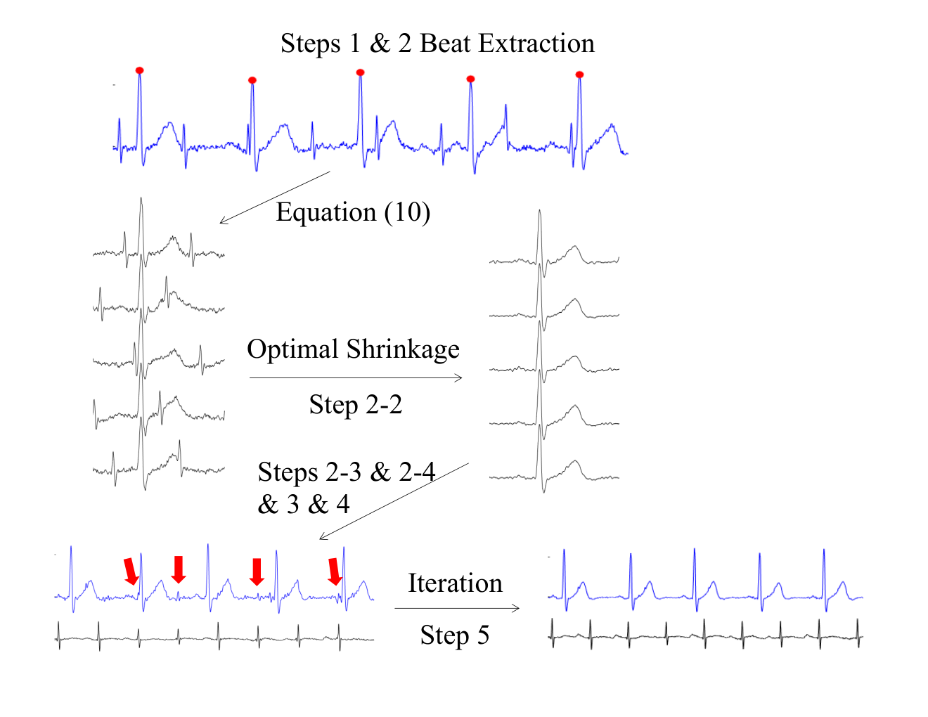
The proposed algorithm falls in the category of single channel blind source separation (scBSS) algorithm for the general purpose. Specifically, the algorithm separates the fetal ECG and maternal ECG out of the recorded ta-mECG. There are three main steps (Steps 2-1, 2-2 and 2-3 below) in addition to the standard pre-processing step (Step 1 below). First, estimate the maternal heart rate based on the nonlinear-type time-frequency analysis called de-shape short-time Fourier transform (dsSTFT) [48, 53]. Then, divide the ta-mECG into pieces so that each piece contains one maternal cardiac cycle. Second, design a metric to compare pieces. The novelty of the proposed algorithm is utilizing the optimal shrinkage (OS) tool that is immune to information not related to the maternal cardiac cycles, like the fetal cardiac activities and noise. With this metric, for each piece, we find other pieces with similar maternal cardiac cycles. Finally, the median of all similar maternal cardiac cycles is evaluated, which recovers the mECG. By repeating these three steps for all pieces, the fECG is recovered. See Figure 2 for a summary illustration of the proposed algorithm. Below we detail the algorithm step by step for the reproducibility purpose.
3.1. Input data
Fix a subject. If the sampling rate of the data from one subject is less than Hz, to enhance the R peak alignment needed in the following steps, the signal is upsampled to Hz [61]. Thus we assume below that all signals are sampled at Hz. Suppose all recordings have simultaneously recorded ta-mECG channels. Denote the -th channel , where and is the number of samples of each channel; that is, the recording is over an interval of seconds.
3.2. Step 1: Preprocessing and linear combination
The Butterworth low-pass filter of order 5 with the cut-off frequency of 100 Hz and a notch filter with the notch centered at 60Hz are applied on each ta-mECG signal to remove high frequency noises and the powerline interference noise. To remove the baseline wandering, which corresponds to low frequency noise caused by a variety of sources including respiration, body movements, and poor electrode contact, we apply the following two stage moving window median filter with window size and ms. This two stage scheme presents higher signal to noise ratio (SNR) in [28] and shows the ability to preserve fECG morphology in [31]. Let and denote the operator of median filter with short and long window size respectively. The baseline wandering of , , is estimated by , and hence the detrended signal .
Following the key idea described in [53], produce a variety of ta-mECG signals constructed by different linear combinations of , . Consider a finite subset , and for each , construct a linear combination:
| (8) |
This construction is based on the dipole current model of ECG signal [58] discussed in Section 2.1. In the following, when , we set , where . Note that when there is only one channel, , and there is no linear combination.
3.3. Step 2-1: Estimate maternal R peaks
In this step we estimate the maternal R peaks. Due to the existence of fetal ECG signal, the traditional R peak detection algorithms might fail. We apply the idea proposed in [48] to obtain the R peaks by taking the beat tracking algorithm into account. We refer readers with interest to [48, 53] for the algorithm details, and [62] for the underlying theory. Denote the collected timestamps of estimated maternal R peak locations of the linearly combined ta-mECG as
| (9) |
where is the timestamp of the -th detected maternal R peak and is the total number of estimated maternal R peaks. As is mentioned in our model, in some linear combinations, it is possible that is too small so that the amplitudes of and are comparable, or even is dominant, which will result in wrong estimation of . To solve this problem, we apply the fusion method [63]. When , out of 14 linear combinations, we collect 5 linear combinations so that the associated detected R peaks have the smallest heart rate variability. Then we apply a voting procedure to determine the final maternal R peaks for all linear combinations. For simplicity, we still denote the final maternal R peaks for each linear combination as .
3.4. Step 2-2. Estimate maternal cardiac cycles by optimal shrinkage
Construct mECG templates. Fix a linear combination , and the -th maternal cardiac cycle determined by the -th R peak. Denote to be the rounding number of the quantile of R to R intervals of . Denote the corresponding ECG segment over the cardiac cycle as
| (10) |
where is the smallest integer larger than and .
Here, the values and are set based on the knowledge of PR and QT duration [64], so that the whole P-QRS-T waveform is covered.
Build up a library for the mECG template, denoted as
.
Remove nuisance variables by optimal shrinkage.
Construct a data matrix of size consisting of all segments of in the columns. To obtain maternal cardiac cycles from , we need to reduce the influence of the fECG and noises. Based on the assumption mentioned in the manifold model, and the low-rank assumption of the mECG inside the data matrix , we
apply the optimal shrinkage [60] as we discussed in 2.2.. Suppose .
Denote the SVD of the data matrix as
| (11) |
where is the matrix rank, and are the -th left and right singular vector corresponding to the singular value , and . Since equation (6) is constructed under the assumption of unit variance of noise level, we normalize with noise level estimated by
| (12) |
where is a constant chosen by the user,
| (13) |
and . We set empirically to avoid underestimating the noise level. Then, we apply the OS as equation (6) as
| (14) |
The columns of are the estimated mECG of each , denoted as .
3.5. Step 2-3. Maternal ECG recovery
After obtaining all estimated maternal cardiac cycles, we reconstruct the estimated mECG signal from by the standard stitching approach [48]. Denote the estimated mECG from as .
3.6. Step 3. Channel Selection by Signal Quality Index
For each linear combination with the estimated mECG , we obtain the rough fECG by a simple subtraction:
| (15) |
Denote to be the collection of rough fECG signals estimated from each linear combination. We apply the bSQI [65] to determine the signal quality index (SQI) for each rough fECG. The optimal linear combination out of , denoted by , is selected as the one that has the highest SQI. From now on, we fix to , and hence to be the rough fECG of the given recording.
3.7. Step 4. Get the fIHR
We repeat Step 2-1 on to acquire the fetal heart beat locations.
3.8. Step 5. Enhance the mECG and rfECG by iteration
Note that to carry out the OS in Step 2-2, we assume that the summation of fECG and noise is a realization of an independent and identical random variable of zero mean, unit variance and finite fourth moment. Recall the underlying theory in Section 2.2. However, this assumption might not be fully satisfies for the fECG. We thus enhance the whole process by iterating Steps 2-2, 2-3 and 4.
Denote the total number of detected fetal R peaks in by . Then repeat Step 2-2 to obtain a set of denoised fetal cardiac cycles, denoted as , where is the -th denoised fetal cardiac cycle. Reconstruct the fECG signal from by the standard stitching approach [48].
Next, improve the mECG estimation by repeating Steps 2-2 and 2-3 on . Note that the fECG component is now suppressed in , so the noise assumption for the OS is better satisfied and we can better recover the mECG, denoted as , and hence the rough fECG, denoted as . Finally, we repeat Step 4 on to acquire the fetal heart beat locations and repeat Step 2-2 on to obtain our proposed estimator of the fECG, denoted as .
3.9. (Optional) Enhance the fECG signal by the nonlocal median
When the fetus is normal sinus rhythmic, we may further improve the fECG morphology by applying the nonlocal median. Denote to be the set of fetal cardiac cycles in . Take , and denote to be those that have the most similar R-R intervals compared with that of . With , we take the entry-wise median of these segments as the estimation of corresponding fetal P-QRS-T waveform; that is, the -th fetal P-QRS-T waveform in is estimated by
| (16) |
Since the median filter is not applied to consecutive cycles, it is called the nonlocal median filter. The nonlocal median filtered fECG is determined by stitching .
4. Material
To validate the proposed algorithm in not only detecting the fetal heart rate, but also recovering the fetal ECG morphology, we use the following databases.
4.1. Real database
The first real database is the database 2013 PhysioNet/Computing in Cardiology Challenge [66]11 1 https://physionet.org/challenge/2013/#data-sets, abbreviated as CinC2013. We focus on the set A, which is composed of 75 recordings with the provided fetal R peak annotations. Each recording includes four ta-mECG channels that were obtained from multiple sources resampled at the sampling rate 1000 Hz and last for 1 minute duration. There is no publicly available information about where the leads are placed on the maternal abdomen. Case a54 is discarded based on the suggestion in [30] since it was discarded by the Challenge organizers. We focus on the remaining 74 recordings.
To demonstrate the performance of recovering fECG morphology, particularly when the fetus is arrhythmic, we also consider the Non-Invasive Fetal ECG Arrhythmia Database (nifeadb) [66]22 2 https://physionet.org/physiobank/database/nifeadb/. The nifeadb contains 12 fetal arrhythmias recordings and 14 normal rhythm recordings. Each recording has one maternal thoracic signals and four or five ta-mECG signals, with the 500 Hz or 1000 Hz sampling rate. The diagnosis information and more details can be found in [9].
4.2. Simulated database
Since there is no gold standard recording of fetal ECG morphology available in any publicly available database, including CinC2013, to validate that our proposed algorithm has the capacity to recover the morphology of fECG from the ta-mECG, we evaluate our algorithm on a set of semi-real simulated ta-mECG data. We consider two databases.
The first one is the MITDB arrhythmia database https://www.physionet.org/physiobank/database/mitdb/, abbreviated as MITDB. This dataset contains 48 half-hour excerpts of two-channel ambulatory ECG recordings, obtained from 47 subjects studied in the Boston’s Beth Israel Hospital Arrhythmia Laboratory between 1975 and 1979. Twenty-three recordings were chosen at random from a set of 4,000 24-hour ambulatory ECG recordings collected from a mixed population of inpatients (about 60%) and outpatients (about 40%) at Boston’s Beth Israel Hospital; the remaining 25 recordings were selected from the same set to include less common but clinically significant arrhythmias that is not well-represented in a small random sample. Each subject has 2 channels with the sampling frequency 360 Hz and the 11-bit resolution over a 10 mV range. The R peak annotations are provided. The second one is the Physikalisch-Technische Bundesanstalt (PTB) Database https://physionet.org/physiobank/database/ptbdb/, abbreviated as PTBDB. The database contains 549 records from 290 subjects aged 17 to 87 with the mean age 57.2. Each subject is represented by one to five records. Each record includes 15 simultaneously measured signals: the conventional 12 leads (I, II, III, AVR, AVL, AVF, V1, V2, V3, V4, V5, V6) together with the Frank lead ECGs (Vx, Vy, Vz). Each signal is digitized with the sampling frequency 1000 Hz and with the 16 bit resolution over a range of mV. Out of 290 subjects, 216 subjects have cardiological disorders, 52 subjects are healthy, and 22 subjects do not have available clinical summary.
To create a mECG in the simulated ta-mECG, we take Vx, Vy, and Vz recordings from healthy subjects in PTBDB, denoted as at time , which are 115 seconds in total. We view the triplet as the maternal vectocardiogram (VCG). We represent the project direction of maternal VCG by a pair of angles, and . The simulated mECG is then created by
| (17) |
Each subject has recordings created with two pairs of directions given by and . In total, 40 mECGs of healthy subjects are generated. Note that in this simulation, we assume that the mECG is arrhythmia-free. The simulated fECG’s of healthy fetus are created from another 40 healthy subjects in the PTBDB, where seconds of the V2 and V4 recordings are taken. The simulated fECG’s of fetus with arrhythmia are created by taking the first seconds from the first and second channel of subjects in the MITDB. The simulated mECG and simulated fECG come from different subjects. Both healthy and arrhythmic signals are resampled at Hz. As a result, the simulated fECG has the same number of data points as the simulated mECG, and has about double the heart rate compared with the simulated mECG if we consider both parts sampled by Hz. The amplitude of the simulated fECG is normalized to the same level of simulated mECG and then multiplied by to make the amplitude smaller then the mECG, consistent with the usual situation of real ta-mECG signals. We generate 40 simulated healthy and arrhythmic fECGs. The clean simulated ta-mECG is generated by directly summing simulated mECG and fECG. The final simulated ta-mECG is generated by adding a Gaussian white noise to the clean simulated ta-mECG according to the assigned signal-to-noise (SNR) ratio. As a result, we acquire recordings of seconds simulated ta-mECG signals with the sampling rate Hz.
We mention that it is likely true that fECG morphology is less diverse compared with adult ECG morphology, in that the QRS duration is narrower, and QRS abnormalities such as bundle branch block, aberrant conduction, polymorphic ventricular ectopy or ventricular tachycardia are less common in the fetus. However, it does not mean that fetus does not have rate-related aberrancy or aberrant conduction following premature atrial beats, and it is not clear how often ventricular ectopy/tachycardia occurs and if this is monomorphic or polymorphic. See, for example, [67, 13], for a report of fetal ventricular ectopy in the setting of complete heart block with and without structural heart disease. If the proposed algorithm could perform well on this more challenging semi-real ta-mECG signal for the morphologic analysis, then it would be reasonable to surmise that it would excel at fetal ECG morphology analysis.
5. Evaluations
5.1. Evaluation of R peak Estimation.
To evaluate the fetal R peak detection performance, a detected R peak is compared with the provided annotations by beat-to-beat comparisons with a matching window of ms [30]; that is, a detected R peak is a true positive if it is close to a true R peak within a ms deviation. We report the score
| (18) |
where TP is the true positive rate (correctly detected R peak), FP is the false positive rate (falsely detected R peak), and FN is the false negative rate (the existing R peak that is not detected). We also compute the mean absolute error (MAE), which is defined by
| (19) |
where is the number of TP detected R peaks, and and are the timestamps of the -th TP detected R peak and the associated true R peak. Here, we follow the common approach [55] to consider only TP R peaks to avoid the evaluation dependence on the R peak detection accuracy. For CinC2013, we report the mean and medium of and MAE for each channel combination over all recordings. For each recording, we evaluate the -quantile, where , of all ’s (respectively MAE’s) of all channel combinations, denoted as (respectively MAE()). Then we report the mean and median of the (respectively MAE()) over all recordings. The practical meaning of (respectively MAE(1)) is the best possible result we can obtain from any combination of channels for a single recording.
5.2. Comparison with other algorithms
When we have more than one channel ta-mECG signals, the fECG decomposition problem falls in the category of the blind source separation (BSS) and its variations [22, 23, 24]. For the comparison purpose, we show the independent component analysis (ICA). There are several approaches to implement ICA, for example, the joint approximation diagonalization of eigen-matrices (JADE), and symmetric and deflationary FAST-ICA approaches. In [55], it is shown that JADE produced slightly better results. Thus, in this work, we only show the JADE result for the ICA approach. We apply the benchmark codes of JADE implementation of ICA provided in http://www.fecgsyn.com, and denote these method as 33 3 Here we follow the nomination proposed in [55].. Another commonly applied method is principle component analysis (PCA). However, as is indicated in [68, Section 3.3.2] that there is no reason for the mECG and fECG to be orthogonal in the observation space, PCA as a BSS approach might not be a suitable approach, so we do not consider it.
A critical step in the BSS approach is identifying the decomposed signal that contains the maternal or fetal ECG [30]. Since there are only two (or three) decomposed signals when we apply to two (or three) ta-mECG channels, it is not feasible to select the optimal channel. For the algorithm, we thus take the ground truth annotation to select the optimal channel that is more likely to be the fECG, and report the detected R peaks from this detected channel. We emphasize that we do not take the ground truth annotation into account in any other algorithms, particularly our proposed algorithm.
When the maternal thoracic-lead ECG signal (mtECG) is available, we can apply the adaptive filter (AF) idea to remove the mECG from the (possibly single channel) ta-mECG, where the maternal thoracic ECG signal (mtECG) is viewed as the reference channel. For example, the least mean square (LMS) [25] or the recursive least square (RLS) [27] and its variations, like the echo state neural network (ESN) [27], blind adaptive filtering [26], extended Kalman filter (EKF) [28], etc. If the mtECG and the mECG in the ta-mECG are linearly related, the LMS or RLS helps to extract the fECG by removing the maternal cardiac activity in the ta-mECG. If the relationship is nonlinear, ESN could help. In our setup, we cannot get the mtECG, so these AF-based algorithms cannot be directly applied. However, recall that we are able to accurately estimate the mECG in the ta-mECG [48, 53]. Therefore, we could view the estimated mECG signal as the reference channel. We mention that this idea is also considered in [33]. Based on this idea, we consider the modified AF-based algorithms proposed in [53]. We replace the direct subtraction step in (15) by the LMS, ESN or EKF, by taking the estimated mECG as the reference channel to get the rough fECG. Note that since other steps are not changed, when there are more than two channels, the bSQI [65] to applied to select the optimal linear combination of multiple channels. Note that this idea can be applied when we have a single channel ta-mECG. We take the publicly available code from http://www.fecgsyn.com for RLS, LMS, ESN and EKF, and follow the suggested parameters accompanying the code. Denote these methods as , , , and respectively.
When we only have a single channel ta-mECG, we compare the proposed algorithm with two benchmark template subtraction (TS) algorithms discussed in [55] and the publicly available code provided in http://www.fecgsyn.com. To run these TS algorithms, we apply Step 2-1 to determine maternal R peaks from the ta-mECG and construct segments associated with all R peaks like (10). For the first TS algorithm, we apply PCA to all segments to determine the principle components. For each segment, the mECG is estimated by selecting suitable principal components and applying a back-propagation step on a beat-to-beat basis. See [55] for details. We denote the first TS algorithm as . For the second TS algorithm, the median of all segments is taken as the template for the mECG. The mECG template is then adapted to each segment using a scalar gain. We denote the second TS algorithm as
Moreover, to appreciate the advantage of the OS step compared with the traditional SVD approach [37, 38, 41], we consider an algorithm that is the same as our proposed algorithm, except (14), where we simply take the top singular vector associated with the largest singular value as the estimated mECG. We denote this algorithm as .
5.3. Evaluation of Morphology Recovery
We evaluate the performance of recovering the fECG morphology on the semi-real simulated ta-mECG signals of healthy fetus, in both the single channel and two channels cases. When there is one channel, the P wave and T peak locations of the simulated fECG and estimated fECG are detected by the algorithm suggested in [64]. When there are two channels, we take the optimal linear combination of two clean simulated fECG’s and the estimated fECG to determine P peaks and T peaks. We view the detected P peak and T peak from the clean simulated fECG as the ground truth. The ECG signals for the clean simulated fECG’s and the detected P peaks and T peaks are visually inspected to confirm the quality of the true annotation. We follow the same way as evaluating the R peak detection by MAE [55] to evaluate the P peak and T peak detection – only those beats with TP R peak detection are considered to evaluate the detected P peak (or T peak). Then the and MAE are also reported.
In addition to reporting the performance of detecting P wave and T peak, we report how the fECG morphology is recovered. The normalized mean amplitude error (NMAE) for R peak morphology recovery is defined as
| (20) |
where is the timestamp of the -th TP estimated R peak, is the timestamp of the associated true R peak, and and represent the whole simulated fECG and its estimation respectively. We also report NMAE for P peaks and T peaks. Similarly, to evaluate the performance of recovering PR (the interval between P peak and R peak), QT (the interval between Q wave and T peak) and ST (the interval between S wave and T peak) intervals, we consider the normalized mean duration error (NMDE):
| (21) |
where is the length of the -th estimated PR interval and is the associated length of the true PR interval. The same formula hold for QT and ST intervals. Again, we follow the same way as evaluating the R peak detection to report NMAE and NMDE – we only consider those beats with TP R peaks to evaluate the estimated peaks and intervals. Clearly, NMAE and NMDE jointly represent how much the morphology of the estimated fECG deviates from the ground truth. The smaller the NMAE and NMDE are, the better the performance of the algorithm. To focus on evaluating the performance of fECG morphology recovery, we take the ground-truth fetal R peak annotation into account to determine which decomposed component is the estimation of the fECG.
6. Results
6.1. Evaluation of R peak location estimation
The performance of the proposed algorithm for 2 channels tested in CinC2013 is summarized in Table 1. The best is , which is achieved in combining channel 1 and channel 4. The associated MAE is msec. On the other hand, the and MAE(1) of all recordings achieves and ms. Clearly, for each recording, if we choose among all combinations, the performance is better. In this table, we also compare the proposed algorithm with SAVER [53] and other algorithms, including , , , , , , , and we see that the proposed algorithm outperforms all other algorithms, including SAVER. Specifically, if we consider the algorithm, that is, we replace the OS step by the top singular vector, the overall performance drops. This indicates the benefit of introducing the OS.
When there are more channels, the proposed algorithm should lead to better results. To confirm this fact, we report the results when we have three channels. The result is summarized in Table 2. The best is , which is achieved when we combine channels 1, 2 and 4. The associated MAE is msec. We see an improvement over the best two-channel combination, channels 1 and 4, when we include channel 2. On the other hand, the and MAE(1) of all recordings achieve and ms. Since there are three channels, we also compare with available blind source separation algorithms. Again, we run the publicly available code provided by [55], and we conclude that our result is consistently better, including and MAE(1).
The proposed algorithm is also applicable when we have only one channel. The result is summarized in Table 3. The best is , which is achieved when channel 2 is considered. The associated MAE is msec. On the other hand, the and MAE(1) of all recordings achieves and ms. Overall, we can see a performance enhancement after introducing OS when compared with the algorithm shown in [48]. We also compare the result with the state-of-the-art template subtraction algorithm. For a fair comparison, we run the publicly available template subtraction code [55]44 4 http://www.fecgsyn.com. Clearly, our result is consistently better over all channels, as well as and MAE(1). Again, the performance of the algorithm, is worse, which again indicates the benefit of the OS step.
To further demonstrate the strength of the proposed algorithm, we consider a more stringent evaluation criteria. In the above reported results, the defined in (18) depends on a matching window of ms [30]. Now we report the based on two smaller matching windows, one of ms and one of ms. The result is shown in Table 4. When the matching window is ms ( ms resp.), the best is ( resp.), which is achieved in combining channel 1 and channel 4. The associated MAE is ( resp.) msec. On the other hand, the and MAE(1) of all recordings achieves and msec ( and msec resp.). Clearly, when the matching window is smaller, the decreases but the MAE also decreases. This result indicates that if we choose the matching window to be msec, the performance is still better than the state-of-the-art algorithm SAVER [53]. Even when the matching window is msec, the result is slightly worse but comparable.
6.2. Demonstration of fECG morphology recovery
See Figure 3 for an illustration of the reconstructed fECG from two single channel simulated ta-mECGs. The SNR is 20dB with the amplitude of the simulated fECG of the simulated mECG in the first case, and the SNR is 10dB with the amplitude of the simulated fECG of the simulated mECG in the second case. Overall, while the morphology is slightly deviated from the simulated one, the main landmarks are easy to identify in the reconstructed signal. We see that even if the maternal and fetal QRS complexes overlap, we can well recover the fetal ECG morphology. However, in some cases, particularly when the fECG amplitude is small and the SNR is low, the morphology may have a large deviation. We can further enhance the rough fECG quality by applying the OS. The results are shown as light red signals in the bottom of Figure 3. We see that the OS does help improve the quality of the rough fECG for the visual inspection purpose.
The decomposition result on the real databases, CinC2013 and nifeadb, are shown in Figures 4 and 5. For the normal fetus from CinC2013, the landmarks P, Q and T can be easily identified, even if the noise level is relatively high for the fECG in the 6-th recording. For the 59-th recording, it is hard to see any fECG in Channel 2 and Channel 3, but after suppressing the mECG by the linear combination idea, we are able to see the fECG in the linearly combined ta-mECG, and hence the extraction of the fECG. In this case, we can see clear P waves in the final recovered fECG, while the T wave is relatively weak.
For the arrhythmic fetus in nifeadb, the results are demonstrated in Figure 5. We show the same cases, ARR 3, ARR 4 and ARR 11, demonstrated in [9, Figures 3, 4 and 5]. In ARR 3, we can easily identify the trigeminy pattern, and the P-waves are visible in most beats, indicated by the blue arrows, allowing perinatal cardiologists to characterize the premature atrial contraction (PACs). Compared with [9, Figure 3], the reconstructed P-waves is more viable from beat to beat. This is expected since we only use two channels. In ARR 4, the blocked P-wave can be easily visualized. Note that compared with the extracted fECG from the multichannel ta-mECG signals shown in [9, Figure 4], the blocked normal P-wave is less clear in our recovery. In ARR 11, the atrial tachycardia with the 2:1 AV conduction can be easily identified. Overall, a side-by-side comparison of the extracted fECG’s by our algorithm with those extracted by the algorithm taking multiple channels into account shown in [9, Figures 3, 4 and 5], we see that the overall quality of our result is not superior but comparable. Particularly, the proposed algorithm could reconstruct most important structure prenatal cardiologists have interest. This result shows the potential of the proposed algorithm for the arrhythmia diagnosis.
6.3. Quantification of fECG morphology recovery
To further quantify the results, , NMAE and NMDE evaluated from the estimated fECG are shown in Figures 6, 7 and 8 under different ratios of fECG and mECG and SNR’s for a direct comparison. Here we follow the report scheme suggested in [55]. In the boxplot, the circle indicates the median, thick line indicates the interquartile range, the dots indicate the outliers, while the thin line indicates the range of the data without the outliers. Here, the outliers are defined as those values that are outside , where and are the -th and -th percentiles of the sample data, and is chosen to be . As expected, the higher the ratio of the fECG and the mECG, and the higher the SNR, the higher the and the lower the NMAE and NMDE. Compared with one channel, the morphology recovery performance is in general better when we have two channels. Since a P wave in general has a smaller amplitude compared with R and T waves, it is not surprising to see that all quantities involving a P wave are less accurate with more outliers and more vulnerable to a small SNR and a small ratio.
7. Discussion and Conclusion
We provide a novel algorithm to recover fECG morphology from few ta-mECG channels. Compared with the traditional algorithms, the main novelty is introducing a new metric to compare cardiac activities based on the OS theory. The algorithm is supported by solid mathematical foundation, and gives a convincing fetal R peak detection result on the publicly available databases compared with those reported in [48, 53, 54], and the fECG morphology recovery result is confirmed on a semi-real simulated database. For the fECG morphology recovery, an important advantage of the proposed algorithm is the ability to recover fECG even when the fetal QRS overlaps a maternal QRS.
7.1. Clinical application and significance
Compared with the state-of-the-art result when we have only few channels [48, 53], the proposed algorithm leads to a more accurate result. This more accurate fetal R peak detection allows better fetal heart rate analysis. Specifically, when two channels are available, the MAE of the best combination is 5.45 4.65 msec. This is equivalent to extracting a R peak to R peak interval from an ECG signal sampled at about 150Hz. With this improvement compared to the state-of-the-art algorithm SAVER when 2 channels are available, we are closer to the recommendation for the ECG sampling rate proposed in [69] for the adult HRV analysis.
To the best of our knowledge, this is the first work showing the possibility to recover the fECG morphology with high accuracy from few ta-mECG channel signals, even when the fetus has an arrhythmia. It has the potential to help fetal ST analysis monitoring that detects and alerts fetal hypoxia, the diagnosis of long QT syndrome that may not result in obvious arrhythmias on echocardiography, and elucidate the origin and mechanisms of tachyarrhythmias and other conditions. Future work will need to focus on real-time clinical data to assess applicability of the method for patient clinical use. Since only few channels are needed, the algorithm has the potential to help long term monitoring of fetal status. This cannot be achieved by periodic fetal echocardiography.
7.2. Comparison with other algorithms
To the best of our knowledge, there are limited algorithms available to analyze fECG when two or three ta-mECG channels are available, except SAVER [53] and the diffusion-based approach [54]. In general, the proposed algorithm falls in the category of the TS method. To have a more systematic comparison and understanding of the relationship, note that the proposed algorithm contains three main ingredients:
- (1)
de-shape short time Fourier transform approach to detect maternal R peaks;
- (2)
linear combination of two or three channels, and the bSQI selection of the best channel;
- (3)
OS approach to determine neighbors for the nonlocal median purpose.
The first ingredient has been extensively discussed in the previous paper [48] and we refer interested readers there. This ingredient is universal and can be combined with other TS methods.
The second ingredient, the linear combination based on the dipole current model, is first proposed in [53] to handle the case when there are only two ta-mECG channels. In [53], the optimal linear combination is determined by combining the lag map and diffusion map [53, (2.2)]. However, we found that a more straightforward bSQI helps determine the optimal linear combination more efficiently – with the bSQI, outperforms SAVER when we have two channels. See Table 1 for details. Thus, in this paper the bSQI is proposed to replace the combination of lag map and diffusion map approach. We mention that this linear combination idea has the potential to be combined with algorithms, like ICA or AF-based algorithms. We will explore this possibility in the future work.
The third ingredient is the main ingredient that can be directly compared with the traditional TS method and its several variations. In the traditional TS method and its variations, the mean, principal components, or singular vectors, of consecutive cardiac activities in the ta-mECG are considered to construct the template of the cardiac activity. These traditional approaches do not take into account the fact that the QRST complex morphology (both maternal and fetal) is time-varying [70]. In the proposed algorithm, we instead model similar QRST complexes located at different time by a low rank model so that the OS can be applied to recover the ECG signal.
7.3. Limitation and future work
The main weak point of this work is the lack of a large scale clinical database with clinical outcome. Specifically, for this study we had to use an existing publicly available benchmark database to demonstrate the potential of the proposed algorithm. While it allows us to compare the fetal R peaks estimation result with other algorithms, it does not contain enough information for us to make further conclusion for the fECG morphology reconstruction. For example, although we have a reasonable reconstruction of PR, ST and QT intervals in the semi-real simulation database with a quantitative measurement in Section 5.3, we do not have the PR, ST or QT interval information commonly used in clinics for the CinC2013 and nifeadb databases. Moreover, while we show several decomposed fECG’s for data in CinC2013 and nifeadb databases in Section 6.2, we do not have a systematic evaluation of the clinical relevance of the reconstructed fECG, like those results shown in [6, 9]. So we cannot conclude how accurate the estimated PR, ST or QT interval is and what clinical information we can provide from the reconstructed fECG morphology. Thus, collecting a large scale and prospective dataset with necessary clinical information and carrying out a clinical application with our clinical team are urgently needed. Moreover, although only two channels are considered, our reconstruction results are in some sense comparable with the results shown in [9, Figures 3, 4 and 5]; specifically, our methods could reconstruct the critical structures. A more systematic study of the nifeadb database, as well as the above-mentioned limitations, will be reported in our future work.
In the simulation, we take the semi-real ta-mECG to evaluate the performance of recovering the fECG morphology by the proposed algorithm. While this semi-real approach is closer to the real world scenario compared with the model-based simulation proposed in [55], it has its own limitation; particularly, note that the projection directions of simulated mECG’s for two channels are fixed, the simulated fECG’s comes from fixed channels, and the respiratory effect on the cardiac axis is not corrected, the simulated signal. Each of these facts may deteriorate the rich physiological dynamics inherited in the real-world ta-mECG. We may combine the model-based simulation [55] to develop a more delicate simulation in the future work.
From the clinical perspective, another unsolved challenge is interpreting the reconstructed fECG signal. Due to the anatomic variation among pregnant women, like uterus position and shape, as well as the fetal size and presentation, even if we could standardize the lead system on the mother’s abdomen, the fECG waveform morphology still varies from subject to subject. Note that the PR interval and QT interval information might be deformed due to this variation, and hence its clinical applicability might be degraded. This situation is more challenging when the gestational age is small. Developing an adaptive algorithm to recover the fetal vectocardiogram for the purpose of establishing an intrinsic fECG lead system is the next challenge we face. From the clinical treatment perspective, we would like to monitor the fECG for medication effects – either medications given to treat the mother or medications given to the mother to treat the fetal arrhythmia. We could monitor fetal heart rates to see if we control the arrhythmia but to the best of our knowledge, so far we have no ability to monitor the effects of medications on fetal conduction.
From the algorithm design perspective, theoretically, we may further take the ECG morphology knowledge into account to design a more robust and accurate OS. This direction involves more theoretical work about “wave-shape manifold” analysis [71]. Due to the nonlocal nature of the proposed algorithm, it can be easily turned into a real-time one for fetal monitoring. Also, when there are multiple channels available, we could modify the proposed algorithm to take all channels into account to achieve a better fECG morphology recovery. Another challenge is an automatic determination of the final fECG estimate from the decomposed two components. This is a commonly encountered channel selection challenge in the BSS algorithm, and usually we need extra information to solve the challenge. In the proposed algorithm, we use a simple approach – select the decomposed component with the smaller median R-R interval as a fECG estimate, and hence the other one as a mECG estimate. However, when the mother has a higher heart rate, particularly when the fetus has a bradycardia, this method would fail. Note that on the bedside, we can count on physicians’ experience to make a decision, but for the real-time diagnosis purpose, we need to find a better criteria to resolve this challenge. In this paper, we follow conventional approach and apply the lowpass filter with the cutoff 100Hz in Step 1. While the proposed algorithm provides an encouraging result, it is not clear how much the lowpass filter impacts the recovered fECG morphology. A more detailed spectral content study of the fECG, following [72], is needed to better understand how to design the optimal lowpass filter to recover the fECG morphology. We leave these challenges to future work.
Reference
References
- [1] R. Weber, D. Stambach, and E. Jaeggib, “Diagnosis and management of common fetal arrhythmias,” Journal of the Saudi Heart Association, vol. 23, no. 2, pp. 61–66, 2011.
- [2] Y. Maeno, A. Hirose, T. Kanbe, and D. Hori, “Fetal arrhythmia: prenatal diagnosis and perinatal management,” Journal of Obstetrics and Gynaecology Research, vol. 35, no. 4, pp. 623–629, 2009.
- [3] M. Cremer, “über die direkte ableitung der aktionstrome des menschlichen herzens vom oesophagus und über das elektrokardiogramm des fetus,” Münchener Medizinische Wochenschrift, vol. 53, pp. 811–813, 1906.
- [4] M. J. Taylor, M. J. Smith, M. Thomas, A. R. Green, F. Cheng, S. Oseku-Afful, L. Y. Wee, N. M. Fisk, and H. M. Gardiner, “Non-invasive fetal electrocardiography in singleton and multiple pregnancies,” BJOG: An International Journal of Obstetrics & Gynaecology, vol. 110, no. 7, pp. 668–678, 2003.
- [5] E. L. Chia, T. F. Ho, M. Rauff, and W. C. Yip, “Cardiac time intervals of normal fetuses using noninvasive fetal electrocardiography,” Prenatal Diagnosis: Published in Affiliation With the International Society for Prenatal Diagnosis, vol. 25, no. 7, pp. 546–552, 2005.
- [6] G. Clifford, R. Sameni, J. Ward, J. Robinson, and A. J. Wolfberg, “Clinically accurate fetal ECG parameters acquired from maternal abdominal sensors,” American Journal of Obstetrics and Gynecology, vol. 205, no. 1, pp. 47.e1–47.e5, 2011.
- [7] J. Behar, T. Zhu, J. Oster, A. Niksch, D. Y. Mah, T. Chun, J. Greenberg, C. Tanner, J. Harrop, R. Sameni, J. Ward, A. J. Wolfberg, and G. D. Clifford, “Evaluation of the fetal QT interval using non-invasive fetal ECG technology,” Physiological Measurement, vol. 37, no. 9, pp. 1392–1403, aug 2016.
- [8] I. Lakhno, J. A. Behar, J. Oster, V. Shulgin, O. Ostras, and F. Andreotti, “The use of non-invasive fetal electrocardiography in diagnosing second-degree fetal atrioventricular block,” Maternal health, neonatology and perinatology, vol. 3, no. 1, p. 14, 2017.
- [9] J. A. Behar, L. Bonnemains, V. Shulgin, J. Oster, O. Ostras, and I. Lakhno, “Noninvasive fetal electrocardiography for the detection of fetal arrhythmias,” Prenatal diagnosis, vol. 39, no. 3, pp. 178–187, 2019.
- [10] G. D. Clifford, I. Silva, J. Behar, and G. B. Moody, “Non-invasive fetal ECG analysis,” Physiological measurement, vol. 35, no. 8, p. 1521, 2014.
- [11] J. F. Strasburger, B. Cheulkar, and R. T. Wakai, “Magnetocardiography for fetal arrhythmias,” Heart Rhythm, vol. 5, no. 7, pp. 1073 – 1076, 2008.
- [12] B. F. Cuneo, J. F. Strasburger, S. Yu, H. Horigome, T. Hosono, A. Kandori, and R. T. Wakai, “In utero diagnosis of long QT syndrome by magnetocardiography,” Circulation, vol. 128, no. 20, pp. 2183–2191, 2013.
- [13] L. K. Hornberger and K. Collins, “New Insights Into Fetal Atrioventricular Block Using Fetal Magnetocardiography,” Journal of the American College of Cardiology, vol. 51, no. 1, pp. 85–86, 2008.
- [14] L. K. Hornberger, “Echocardiographic assessment of fetal arrhythmias,” Heart, vol. 93, no. 11, pp. 1331–1333, 2007.
- [15] M. A. Belfort, G. R. Saade, and et. al., “A randomized trial of intrapartum fetal ECG ST-segment analysis,” N. Engl. J. Med., vol. 373, no. 7, pp. 632–641, 2015.
- [16] H. M. Jenkins, “Thirty years of electronic intrapartum fetal heart rate monitoring: discussion paper,” J. R. Soc. Med., vol. 82, no. 4, pp. 210–4, 1989.
- [17] R. Sameni and G. D. Clifford, “A review of fetal ECG signal processing; issues and promising directions,” Open Pacing Electrophysiol Ther J., vol. 3, pp. 4–20, 2010.
- [18] L. De Lathauwer, B. De Moor, and J. Vandewalle, “Fetal Electrocardiogram Extraction by Blind Source Subspace Separation,” IEEE Trans. Biomed. Eng., vol. 47, no. 5, pp. 567–572, 2000.
- [19] M. Akhbari, M. Niknazar, C. Jutten, M. B. Shamsollahi, and B. Rivet, “Fetal Electrocardiogram R-peak Detection using Robust Tensor Decomposition and Extended Kalman Filtering,” Computing in Cardiology, pp. 189–192, 2013.
- [20] C. Di Maria, C. Liu, D. Zheng, A. Murray, and P. Langley, “Extracting fetal heart beats from maternal abdominal recordings: selection of the optimal principal components.” Physiol. Meas., vol. 35, no. 8, pp. 1649–64, 2014.
- [21] M. Varanini, G. Tartarisco, L. Billeci, A. Macerata, G. Pioggia, and R. Balocchi, “An efficient unsupervised fetal QRS complex detection from abdominal maternal ECG,” Physiol. Meas., vol. 35, no. 8, pp. 1607–19, 2014.
- [22] R. Sameni, C. Jutten, and M. Shamsollahi, “Multichannel electrocardiogram decomposition using periodic component analysis,” IEEE Trans. Biomed. Eng., vol. 55, no. 8, pp. 1935–1940, 2008.
- [23] M. Haghpanahi and D. A. Borkholder, “Fetal ECG Extraction From Abdominal Recordings using Array Signal Processing,” Computing in Cardiology, vol. 40, pp. 173–176, 2013.
- [24] H. Akbari, M. B. Shamsollahi, and R. Phlypo, “Fetal ECG Extraction using Tucker Decomposition,” in International Conference on Systems, Signals and Image Processing. IEEE, 2015.
- [25] B. Widrow, C. S. Williams, J. R. Glover, J. M. McCool, R. H. Hearn, J. R. Zeidler, J. Kaunitz, E. Dong, and R. C. Goodlin, “Adaptive Noise Cancelling: Principles and Applications,” Proceedings of the IEEE, vol. 63, no. 12, pp. 1692–1716, 1975.
- [26] D. Graupe, M. H. Graupe, Y. Zhong, and R. K. Jackson, “Blind adaptive filtering for non-invasive extraction of the fetal electrocardiogram and its non-stationarities,” Proc. Inst. Mech. Eng. H J. Eng. Med., vol. 222, no. 8, pp. 1221–1234, 2008.
- [27] J. Behar, A. Johnson, G. D. Clifford, and J. Oster, “A comparison of single channel fetal ECG extraction methods,” Ann Biomed Eng, vol. 42, no. 6, pp. 1340–1353, 2014.
- [28] R. Sameni, “Extraction of fetal cardiac signals from an array of maternal abdominal recordings,” Ph.D. dissertation, Sharif University of Technology – Institut National Polytechnique de Grenoble, 2008.
- [29] M. Niknazar, B. Rivet, and C. Jutten, “Fetal ECG extraction by extended state Kalman filtering based on single-channel recordings,” IEEE Trans. Biomed. Eng., vol. 60, no. 5, pp. 1345–52, 2013.
- [30] F. Andreotti, M. Riedl, T. Himmelsbach, D. Wedekind, N. Wessel, H. Stepan, C. Schmieder, A. Jank, H. Malberg, and S. Zaunseder, “Robust fetal ECG extraction and detection from abdominal leads.” Physiol. Meas., vol. 35, no. 8, pp. 1551–67, 2014.
- [31] D. Panigrahy and P. K. Sahu, “Extraction of fetal ECG signal by an improved method using extended Kalman smoother framework from single channel abdominal ECG signal,” Australasian Physical & Engineering Sciences in Medicine, vol. 40, no. 1, pp. 191–207, Mar 2017.
- [32] A. Ghaffari, M. J. Mollakazemi, S. A. Atyabi, and M. Niknazar, “Robust fetal QRS detection from noninvasive abdominal electrocardiogram based on channel selection and simultaneous multichannel processing,” Australas Phys Eng Sci Med, vol. 38, no. 4, pp. 581–592, 2015.
- [33] R. Rodrigues, “Fetal beat detection in abdominal ECG recordings: global and time adaptive approaches.” Physiol. Meas., vol. 35, no. 8, pp. 1699–711, 2014.
- [34] J. A. Lipponen and M. P. Tarvainen, “Advanced Maternal ECG Removal and Noise Reduction for Application of Fetal QRS Detection,” Computing in Cardiology, vol. 40, pp. 161–164, 2013.
- [35] A. Damen and J. Van Der Kam, “The use of the singular value decomposition in electrocardiography,” Medical and Biological Engineering and Computing, vol. 20, no. 4, pp. 473–482, 1982.
- [36] S. Cerutti, G. B. Baselli, S. Civardi, E. Ferrazzi, A. M. Marconi, M. Pagani, and G. Pardi, “Variability analysis of fetal heart rate signals as obtained from abdominal electrocardiographic recordings,” J Perinat Med, vol. 14, no. 6, pp. 445–452, 1986.
- [37] A. van Oosterom, “Spatial filtering of the fetal electrocardiogram,” Journal of Perinatal Medicin, vol. 14, no. 6, pp. 411–419, 1986.
- [38] J. Vanderschoot, D. Callaerts, W. Sansen, J. Vandewalle, G. Vantrappen, and J. Janssens, “Two methods for optimal mecg elimination and fecg detection from skin electrode signals,” IEEE Transaction on Biomedical Engineering, vol. 34, no. 3, pp. 233–243, 1987.
- [39] S. M. M. Martens, C. Rabotti, M. Mischi, and R. J. Sluijter, “A Robust Fetal ECG Detection Method for Abdominal Recordings.” Physiol. Meas., vol. 28, pp. 373–88, 2007.
- [40] M. Ungureanu, J. W. M. Bergmans, S. G. Oei, and R. Strungaru, “Fetal ECG extraction during labor using an adaptive maternal beat subtraction technique,” Biomedizinische Technik, vol. 52, no. 1, pp. 56–60, 2007.
- [41] P. P. Kanjilal, S. Palit, and G. Saha, “Fetal ECG extraction from single-channel maternal ECG using singular value decomposition,” IEEE Trans. Biomed. Eng., vol. 44, no. 1, pp. 51–59, 1997.
- [42] I. Christov, I. Simova, and R. Abächerli, “Extraction of the fetal ECG in noninvasive recordings by signal decompositions.” Physiol. Meas., vol. 35, pp. 1713–21, 2014.
- [43] A. H. Khamene and S. Negahdaripoure, “A new method for the extraction of fetal ECG from the composite abdominal signal,” IEEE Trans. Biomed. Eng., vol. 47, no. 4, pp. 507–516, 2000.
- [44] E. C. Karvounis, M. G. Tsipouras, D. I. Fotiadis, and K. K. Naka, “An automated methodology for fetal heart rate extraction from the abdominal electrocardiogram,” IEEE Trans Inf Technol Biomed, vol. 11, no. 6, pp. 628–638, 2007.
- [45] E. Castillo, D. P. Morales, G. Botella, A. Garcia, L. Parrilla, and A. J. Palma, “Efficient wavelet-based ECG processing for single-lead FHR extraction,” Digital Signal Processing, vol. 23, no. 6, pp. 1897–1909, 2013.
- [46] R. Almeida, H. Gonçalves, J. Bernardes, and A. P. Rocha, “Fetal QRS detection and heart rate estimation: a wavelet-based approach.” Physiol. Meas., vol. 35, no. 8, pp. 1723–35, 2014.
- [47] G. Lamesgin, Y. Kassaw, and D. Assefa, “Extraction of Fetal ECG from Abdominal ECG and Heart Rate Variability Analysis,” Advances in Intelligent Systems and Computing, vol. 334, pp. 147–161, 2015.
- [48] L. Su and H.-T. Wu, “Extract fetal ecg from single-lead abdominal ecg by de-shape short time fourier transform and nonlocal median,” Frontiers in Applied Mathematics and Statistics, vol. 3, p. 2, 2017.
- [49] K. Lee and B. Lee, “Sequential Total Variation Denoising for the Extraction of Fetal ECG from Single-Channel Maternal Abdominal ECG,” Sensors, vol. 16, no. 7, p. 1020, 2016.
- [50] M. Richter, T. Schreiber, and D. Kaplan, “Fetal ECG extraction with nonlinear state-space projections,” IEEE Trans. Biomed. Eng., vol. 45, no. 1, pp. 133–137, 1998.
- [51] E. C. Karvounis and M. G. Tsipouras, “Detection of Fetal Heart Rate Through 3-D Phase Recordings,” IEEE Trans. Biomed. Eng., vol. 56, no. 5, pp. 1394–1406, 2009.
- [52] M. Kotas, J. Jezewski, A. Matonia, and T. Kupka, “Towards noise immune detection of fetal QRS complexes,” Comput Methods Programs Biomed, vol. 97, no. 3, pp. 241–256, 2010.
- [53] R. Li, M. G. Frasch, and H.-T. Wu, “Efficient fetal-maternal ecg signal separation from two channel maternal abdominal ecg via diffusion-based channel selection,” Frontiers in Physiology, vol. 8, p. 277, 2017.
- [54] T. Shnitzer, M. Ben-Chen, L. Guibas, R. Talmon, and H.-T. Wu, “Recovering hidden components in multimodal data with composite diffusion operators,” SIAM Journal on Mathematics of Data Science (Accepted for publication), 2019.
- [55] F. Andreotti, J. Behar, S. Zaunseder, J. Oster, and G. D. Clifford, “An open-source framework for stress-testing non-invasive foetal ECG extraction algorithms,” Physiol. Meas., vol. 37, no. 5, pp. 627–648, 2016.
- [56] E. Fotiadou, J. van Laar, S. Oei, and R. Vullings, “Enhancement of low-quality fetal electrocardiogram based on time-sequenced adaptive filtering,” Medical & Biological Engineering & Computing, vol. 56, pp. 2313–2323, 2018.
- [57] R. Vullings, B. de Vries, and J. Bergmans, “An adaptive kalman filter for ecg signal enhancement,” IEEE Trans Biomed Eng, vol. 58, no. 4, pp. 1094–1103, 2011.
- [58] J. Keener, Mathematical Physiology. Springer, 1998.
- [59] R. Sameni, C. Jutten, and M. B. Shamsollahi, “What ica provides for ecg processing: Application to noninvasive fetal ecg extraction,” in 2006 IEEE International Symposium on Signal Processing and Information Technology. IEEE, 2006, pp. 656–661.
- [60] M. Gavish and D. L. Donoho, “Optimal Shrinkage of Singular Values,” IEEE Transactions on Information theory, vol. 63, no. 4, pp. 2137–2152, 2017.
- [61] P. Laguna and L. Sörnmo, “Sampling rate and the estimation of ensemble variability for repetitive signals.” Medical & biological engineering & computing, vol. 38, no. 5, pp. 540–6, 2000.
- [62] C.-Y. Lin, L. Su, and H.-T. Wu, “Wave-shape function analysis – when cepstrum meets time–frequency analysis,” Journal of Fourier Analysis and Applications, vol. 24, no. 2, pp. 451–505, 2018.
- [63] Q. Yu, Q. Guan, P. Li, T.-B. Liu, X.-L. Huang, Y. Zhao, H.-X. Liu, and Y.-Q. Wang, “Fusion of detected multi-channel maternal electrocardiogram (ECG) r-wave peak locations,” Biomedical engineering online, vol. 15, no. 1, p. 4, 2016.
- [64] M. Elgendi, M. Meo, and D. Abbott, “A proof-of-concept study: Simple and effective detection of P and T waves in arrhythmic ecg signals,” Bioengineering, vol. 3, no. 4, 2016.
- [65] A. E. W. Johnson, J. Behar, F. Andreotti, G. D. Clifford, and J. Oster, “Multimodal heart beat detection using signal quality indices,” Physiol. Meas., vol. 36, no. 8, pp. 1665–77, 2015.
- [66] A. Goldberger, L. Amaral, L. Glass, J. Hausdorff, P. Ivanov, R. Mark, J. Mietus, G. Moody, C.-K. Peng, and H. Stanley, “Physiobank, physiotoolkit, and physionet: Components of a new research resource for complex physiologic signals.” Circulation, vol. 101, no. 23, pp. e215–e220, 2000.
- [67] H. Zhao, B. F. Cuneo, J. F. Strasburger, J. C. Huhta, N. L. Gotteiner, and R. T. Wakai, “Electrophysiological Characteristics of Fetal Atrioventricular Block,” Journal of the American College of Cardiology, vol. 51, no. 1, pp. 77–84, 2008.
- [68] J. Behar, “Extraction of clinical information from the non-invasive fetal electrocardiogram,” Ph.D. dissertation, Oxford University, 2014.
- [69] Task Force, “Heart Rate Variability : Standards of Measurement, Physiological Interpretation, and Clinical Use,” Circulation, vol. 93, no. 5, pp. 1043–1065, 1996.
- [70] M. Malik, P. Farbom, V. Batchvarov, K. Hnatkova, and A. Camm, “Relation between QT and RR intervals is highly individual among healthy subjects: implications for heart rate correction of the QT interval,” Heart, vol. 87, no. 3, pp. 220–228, 2002.
- [71] Y.-T. Lin, J. Malik, and H.-T. Wu, “Wave-shape oscillatory model for biomedical time series with applications,” arXiv preprint arXiv:1907.00502, 2019.
- [72] S. Abboud and D. Sadeh, “Spectral analysis of the fetal electrocardiogram,” Computers in Biology and Medicine, vol. 19, no. 6, pp. 409–415, 1989.
| channels | SAVER [53] | Proposed | ||
| (%) | 1+2 | 81.69 25.82 | 86.62 23.34 | 61.05 33.03 |
| 1+3 | 82.93 26.28 | 89.72 21.76 | 57.18 31.88 | |
| 1+4 | 87.93 22.64 | 93.21 14.31 | 63.93 32.42 | |
| 2+3 | 74.40 30.63 | 79.25 31.75 | 58.01 33.85 | |
| 2+4 | 81.50 26.64 | 87.32 24.44 | 62.28 32.16 | |
| 3+4 | 79.83 28.49 | 82.60 28.03 | 56.23 32.90 | |
| (%) | 92.9916.00 | 96.31 10.93 | 73.60 27.73 | |
| (%) | 85.43 22.42 | 87.94 21.30 | 62.32 30.28 | |
| MAE (ms) | 1+2 | 7.72 7.03 | 6.86 6.55 | 11.02 9.30 |
| 1+3 | 7.83 7.45 | 6.43 6.37 | 11.60 9.21 | |
| 1+4 | 6.21 6.03 | 5.44 4.18 | 9.77 8.75 | |
| 2+3 | 9.44 6.88 | 8.61 7.51 | 12.53 9.66 | |
| 2+4 | 7.93 6.62 | 7.11 6.77 | 10.59 8.39 | |
| 3+4 | 7.85 6.85 | 7.27 7.29 | 12.51 9.21 | |
| MAE(1) (ms) | 5.38 4.52 | 4.933.64 | 8.29 7.68 | |
| MAE(0.5) (ms) | 6.54 4.92 | 6.37 5.71 | 9.69 7.46 | |
| channels | ||||
| (%) | 1+2 | 48.27 35.61 | 44.19 34.28 | 83.87 27.53 |
| 1+3 | 49.47 35.35 | 48.73 34.48 | 84.83 26.47 | |
| 1+4 | 55.85 36.10 | 55.47 35.26 | 89.48 21.76 | |
| 2+3 | 51.41 35.84 | 48.71 36.56 | 81.61 29.06 | |
| 2+4 | 55.62 35.51 | 53.37 35.92 | 84.07 27.96 | |
| 3+4 | 48.00 33.62 | 48.92 33.28 | 78.64 31.44 | |
| (%) | 63.2334.22 | 65.18 31.93 | 91.9519.43 | |
| (%) | 52.62 34.29 | 50.7234.04 | 87.10 21.95 | |
| MAE (ms) | 1+2 | 15.67 9.79 | 15.94 9.86 | 9.58 7.30 |
| 1+3 | 16.26 10.33 | 16.00 10.17 | 9.59 7.07 | |
| 1+4 | 12.89 9.45 | 12.60 9.65 | 8.65 6.09 | |
| 2+3 | 15.03 9.50 | 14.82 8.81 | 9.89 7.92 | |
| 2+4 | 12.61 9.51 | 12.93 9.41 | 9.15 7.20 | |
| 3+4 | 15.49 9.57 | 14.82 9.01 | 10.52 8.24 | |
| MAE(1) (ms) | 11.70 9.46 | 10.92 8.73 | 7.93 5.98 | |
| MAE(0.5) (ms) | 13.88 9.12 | 13.55 8.65 | 8.82 6.31 | |
| channels | ||||
| (%) | 1+2 | 83.43 27.78 | 40.92 32.69 | 79.19 31.56 |
| 1+3 | 83.61 27.75 | 38.55 31.89 | 75.26 33.85 | |
| 1+4 | 90.20 18.80 | 40.96 33.21 | 83.57 28.20 | |
| 2+3 | 79.53 30.65 | 38.33 31.41 | 75.38 34.29 | |
| 2+4 | 84.19 27.95 | 38.35 31.56 | 78.00 33.55 | |
| 3+4 | 79.53 30.10 | 36.92 30.73 | 73.45 36.54 | |
| (%) | 94.4213.66 | 39.01 27.31 | 88.3125.28 | |
| (%) | 85.95 23.13 | 38.5029.44 | 80.7730.16 | |
| MAE (ms) | 1+2 | 7.60 7.57 | 18.91 9.06 | 8.55 8.17 |
| 1+3 | 8.28 8.39 | 19.19 8.66 | 9.82 9.10 | |
| 1+4 | 6.11 5.57 | 18.32 9.92 | 7.80 8.02 | |
| 2+3 | 8.78 7.81 | 19.32 8.54 | 10.06 8.75 | |
| 2+4 | 7.98 7.69 | 19.10 8.95 | 8.98 8.55 | |
| 3+4 | 8.33 7.93 | 19.28 8.76 | 10.15 9.25 | |
| MAE(1) (ms) | 5.28 4.01 | 16.33 9.75 | 7.00 7.45 | |
| MAE(0.5) (ms) | 6.80 6.15 | 18.97 8.45 | 8.097.68 | |
| channels | SAVER [53] | Proposed | ||||
| (%) | 1+2+3 | 80.68 29.52 | 89.70 23.46 | 86.33 25.81 | 77.05 34.90 | 22.31 16.50 |
| 1+2+4 | 84.53 26.22 | 93.91 14.83 | 87.24 25.46 | 75.24 35.33 | 25.74 23.69 | |
| 1+3+4 | 83.52 27.98 | 93.62 14.57 | 88.08 23.47 | 80.73 31.86 | 26.66 24.02 | |
| 2+3+4 | 77.51 31.47 | 84.82 27.31 | 80.28 31.23 | 78.01 34.01 | 24.51 21.04 | |
| (%) | 91.20 18.47 | 95.32 13.75 | 89.64 22.94 | 87.16 26.77 | 33.8330.07 | |
| (%) | 82.7926.67 | 91.90 17.38 | 86.8125.06 | 79.50 32.15 | 24.09 19.23 | |
| MAE (ms) | 1+2+3 | 7.15 6.29 | 6.75 7.28 | 6.11 5.05 | 9.74 8.61 | 21.95 5.28 |
| 1+2+4 | 6.44 6.13 | 5.64 5.11 | 6.48 6.76 | 9.68 9.56 | 21.38 7.02 | |
| 1+3+4 | 6.73 6.43 | 5.47 5.09 | 6.11 5.79 | 8.87 8.48 | 20.25 7.47 | |
| 2+3+4 | 7.97 7.08 | 7.82 7.23 | 8.12 8.00 | 9.39 9.01 | 21.61 6.37 | |
| MAE(1) (ms) | 5.22 3.87 | 5.41 5.22 | 5.77 5.23 | 7.58 7.85 | 22.27 8.39 | |
| MAE(0.5) (ms) | 6.67 5.68 | 5.80 5.36 | 6.326.02 | 8.798.24 | 21.76 5.85 | |
| channel | [48] | Proposed | ||
| (%) | 1 | 68.38 33.12 | 66.29 36.76 | 63.57 35.50 |
| 2 | 74.35 29.96 | 75.63 30.96 | 72.47 33.17 | |
| 3 | 64.10 33.58 | 65.75 35.09 | 62.36 36.33 | |
| 4 | 75.68 29.64 | 74.70 32.40 | 71.92 34.12 | |
| (%) | 87.0122.06 | 88.05 23.08 | 83.72 26.27 | |
| (%) | 74.06 27.63 | 72.67 29.92 | 69.6231.83 | |
| MAE (ms) | 1 | 11.33 9.31 | 11.79 9.62 | 12.059.69 |
| 2 | 9.86 7.99 | 8.97 7.77 | 10.538.84 | |
| 3 | 12.17 9.04 | 12.49 9.48 | 12.959.43 | |
| 4 | 8.98 7.95 | 9.06 8.50 | 9.948.81 | |
| MAE(1) (ms) | 5.88 5.14 | 6.085.41 | 7.097.21 | |
| MAE(0.5) (ms) | 9.56 6.86 | 9.69 7.37 | 10.57 7.87 | |
| channel | ||||
| (%) | 1 | 61.17 37.63 | 62.64 38.08 | 61.33 35.34 |
| 2 | 64.47 36.95 | 64.57 36.31 | 67.67 35.88 | |
| 3 | 55.55 37.02 | 56.97 36.78 | 57.32 37.54 | |
| 4 | 67.45 36.34 | 69.08 35.23 | 68.24 35.06 | |
| (%) | 82.7329.32 | 84.47 27.75 | 82.3128.05 | |
| (%) | 68.53 33.13 | 68.36 33.16 | 70.8132.13 | |
| MAE (ms) | 1 | 12.88 10.23 | 12.29 9.68 | 14.63 8.27 |
| 2 | 11.16 8.64 | 10.72 8.30 | 12.22 8.21 | |
| 3 | 13.69 9.55 | 13.25 9.67 | 14.64 8.43 | |
| 4 | 9.30 8.26 | 8.94 8.00 | 12.15 8.03 | |
| MAE(1) (ms) | 6.84 6.91 | 6.646.61 | 9.96 7.24 | |
| MAE(0.5) (ms) | 11.37 8.58 | 11.35 8.52 | 12.537.89 | |
| channel | ||||
| (%) | 1 | 43.04 31.50 | 45.76 34.42 | 47.24 33.91 |
| 2 | 50.87 32.80 | 53.57 35.21 | 51.73 35.09 | |
| 2 | 43.67 33.51 | 45.30 36.43 | 45.15 34.98 | |
| 4 | 49.35 34.23 | 51.78 35.27 | 50.19 34.04 | |
| (%) | 63.7931.80 | 67.34 33.10 | 68.3231.27 | |
| (%) | 47.50 30.16 | 54.43 33.62 | 53.7933.06 | |
| MAE (ms) | 1 | 15.46 9.18 | 14.37 9.65 | 14.23 9.35 |
| 2 | 12.94 8.74 | 11.45 8.17 | 12.67 8.72 | |
| 3 | 15.23 8.11 | 14.95 9.34 | 13.63 8.38 | |
| 4 | 13.33 9.00 | 12.14 9.38 | 12.52 9.64 | |
| MAE(1) (ms) | 10.21 8.70 | 8.927.58 | 8.13 6.67 | |
| MAE(0.5) (ms) | 13.76 7.26 | 12.25 8.25 | 12.388.18 | |
| channels | 10 ms | 25 ms | 50 ms | |
| (%) | 1+2 | 77.45 29.80 | 82.77 27.61 | 86.62 23.54 |
| 1+3 | 81.15 26.55 | 86.2724.51 | 89.72 21.76 | |
| 1+4 | 84.15 20.65 | 89.9516.98 | 93.21 14.31 | |
| 2+3 | 69.13 34.83 | 75.0434.20 | 79.25 31.75 | |
| 2+4 | 78.30 28.69 | 83.2127.13 | 87.32 24.44 | |
| 3+4 | 75.08 32.21 | 78.6731.09 | 82.60 28.03 | |
| (%) | 90.6714.83 | 94.05 13.16 | 96.31 10.93 | |
| (%) | 79.78 25.05 | 84.44 23.94 | 87.94 21.30 | |
| MAE (ms) | 1+2 | 3.39 2.13 | 4.503.26 | 6.86 6.55 |
| 1+3 | 3.58 2.09 | 4.433.01 | 6.43 6.37 | |
| 1+4 | 3.36 2.15 | 4.042.60 | 5.44 4.18 | |
| 2+3 | 3.82 1.99 | 5.543.69 | 8.61 7.51 | |
| 2+4 | 3.45 1.90 | 4.703.18 | 7.11 6.77 | |
| 3+4 | 3.27 2.05 | 4.503.39 | 7.27 7.29 | |
| MAE(1) (ms) | 3.211.99 | 3.922.50 | 4.933.64 | |
| MAE(0.5) (ms) | 3.38 1.85 | 4.362.54 | 6.37 5.71 | |