The digest2 NEO Classification CodeJournal: PASP, Day Month Year

Sonia Keys Affiliation: Harvard-Smithsonian Center for Astrophysics, 60 Garden St., MS 51, Cambridge, MA 02138, USA Peter Vereš Affiliation: Harvard-Smithsonian Center for Astrophysics, 60 Garden St., MS 51, Cambridge, MA 02138, USA Email: peter.veres@cfa.harvard.edu Corresponding author: Peter Vereš Matthew J. Payne OrcID: 0000-0001-5133-6303 Affiliation: Harvard-Smithsonian Center for Astrophysics, 60 Garden St., MS 51, Cambridge, MA 02138, USA Matthew J. Holman OrcID: 0000-0002-1139-4880 Affiliation: Harvard-Smithsonian Center for Astrophysics, 60 Garden St., MS 51, Cambridge, MA 02138, USA Robert Jedicke Affiliation: Institute for Astronomy, 2680 Woodlawn Drive, Honolulu, HI 96822, USA Gareth V. Williams Affiliation: Harvard-Smithsonian Center for Astrophysics, 60 Garden St., MS 51, Cambridge, MA 02138, USA Tim Spahr Affiliation: NEO Sciences, LLC, 1308 Applebriar Lane, Marlborough, MA 01752, USA David J. Asher OrcID: 0000-0003-0423-7112 Affiliation: Armagh Observatory and Planetarium, College Hill, Armagh, BT61 9DG, UK Carl Hergenrother Affiliation: Lunar and Planetary Laboratory, University of Arizona, Tucson, AZ 85721, USA

Abstract

We describe the digest2 software package, a fast, short-arc orbit classifier for small Solar System bodies. The digest2 algorithm has been serving the community for more than 13 years. The code provides a score, $D_{2}{}$ , which represents a pseudo-probability that a tracklet belongs to a given Solar System orbit type. digest2 is primarily used as a classifier for Near-Earth Object (NEO) candidates, to identify those to be prioritized for follow-up observation. We describe the historical development of digest2 and demonstrate its use on real and synthetic data. We find that digest2 can accurately and precisely distinguish NEOs from non-NEOs. At the time of detection, 14% of NEO tracklets and 98.5% of non-NEOs tracklets have $D_{2}{}$ below the critical value of $D_{2}{}=65$ . 94% of our simulated NEOs achieved the maximum $D_{2}=100$ and 99.6% of NEOs achieved $D_{2}{}\geq 65$ at least once during the simulated 10-year timeframe. We demonstrate that $D_{2}{}$ varies as a function of time, rate of motion, magnitude and sky-plane location, and show that NEOs tend to have lower $D_{2}{}$ at low Solar elongations close to the ecliptic. We use our findings to recommend future development directions for the digest2 code.

Keywords:

short-arc orbit determination, asteroids, Near-Earth Object, Minor Planet Center

I Introduction

Near-Earth Objects (NEOs), defined as any small Solar System body having perihelion less than 1.3 $\,\mathrm{au}$ , are of significant interest for a number of reasons. These include planetary defense, spacecraft missions, commercial development, and investigations into the origin and evolution of the Solar System. The NEO discovery rate has risen rapidly in recent decades, driven by the 1998 Congressional mandate to discover 90% of NEOs larger than 1 km (Morrison 1992, the Spaceguard Survey), and the subsequent 2005 Congressional mandate to discover 90% of NEOs larger than 140 m (George E. Brown, Jr. NEO Survey Act ¹¹ 1 Section 321 of the NASA Authorization Act of 2005 (Public Law No. 109-155)).

Solar System objects are typically identified through their apparent motion in a series of images spanning minutes to hours. Given such a sequence of exposures, it is straightforward to identify “tracklets” (Kubica et al. 2007), sets of detections that are consistent with an object with a fixed rate of motion. A related term is an arc, which may contain any number of tracklets, possibly from different observatories. The time span from first to last observation is termed the arc-length.

It is straightforward to determine whether a tracklet represents a known object with a well defined orbit. In that case, the observations coincide with the predicted positions for the known object. Otherwise, the tracklet likely represents a newly discovered object. It is then of interest to determine what type of orbit that object has, and in particular, if it is a new NEO. Given limited telescopic resources, it is not possible to re-observe all objects to immediately determine their orbits. It is therefore essential to identify which objects are more likely to be NEOs and prioritize those for further observation.

Although a tracklet does not uniquely determine an orbit, characteristic sky-plane motion can be used to infer a possible orbit type (Jedicke 1996, e.g.). The tool currently used for this is digest2²² 2 There is no known history of a digest1; this is not version 2 of a program. Also nothing is known about the origin or meaning of the name. The program name is simply digest2.. The digest2 code uses only a single motion vector, derived from a tracklet or short arc, to identify all possible elliptical orbits consistent with that motion. This set of possible orbits is then divided into disjoint orbital categories. Given a population model that represents the number of solar system objects of each type, we can estimate the likelihood that the tracklet represent a member of each category.

With a suitable threshold, digest2 can serve as an NEO binary classifier. Tracklets with high $\emph{digest2}{}$ scores, $D_{2}{}$ , are posted on the Near-Earth Object Confirmation Page (NEOCP³³ 3 http://www.minorplanetcenter.net/iau/NEO/toconfirm_tabular.html). These objects are prioritized by the NEO follow-up community for additional observations.

In this manuscript we describe the digest2 code. The code as implemented has been used by the community for a number of years. Our primary goal is to describe and document the major elements of digest2 and the practical consequences of its design and implementation. Although we highlight possible areas of improvement, these are left for future work.

II Methodology

The observations from a short-arc tracklet directly constrain the position, $(\alpha,\delta)$ , and motion, $(\dot{\alpha},\dot{\delta})$ , of the asteroid in the sky, but the topocentric radial-distance, $\rho$ , and radial-velocity, $\dot{\rho}$ , between the asteroid and the observer are essentially unconstrained. This is the fundamental challenge of orbit determination.

An assumed $\rho$ allows a heliocentric position to be derived (see Appendix A), and with the assumption of a topocentric $\dot{\rho}$ , a heliocentric velocity can also be calculated. Milani et al. 2004 refer to the “admissible region” as being the set of $(\rho,\dot{\rho})$ for which the resultant orbit is heliocentrically bound (elliptical w.r.t. the Sun).

Many authors have addressed the problem of short-arc orbit determination and constraint (e.g. Väisälä 1939; Marsden 1985; Bowell 1989; Bowell et al. 1990; Marsden 1991; Tholen & Whiteley 2000; Milani et al. 2004; Milani & Knežević 2005; Oszkiewicz et al. 2009; Spoto et al. 2018, and discussions therein). Of particular relevance to digest2, in the late 1980s and early 1990s, R. H. McNaught of the Siding Spring Observatory undertook an extensive effort to determine allowable orbital element ranges and class-specific object probabilities based on two observations and a magnitude (McNaught 1999, Pangloss). The method proceeded by stepping through a range of possible topocentric distances and angles (between the velocity vector and the line of sight) which were consistent with the observations and bound to the sun. Pangloss used a population model to assign weights to different orbit classes. The Pangloss code provided the foundation for the digest2 code described in this manuscript.

We review two related methods for addressing the problem of short-arc orbits. The first concerns the technique referred to as “statistical ranging” (Virtanen et al. 2001), in which two observations are selected from the tracklet, thus fixing $(\alpha,\dot{\alpha},\delta,\dot{\delta})$ , and then topocentric ranges at each of the epochs of the two observations are randomly chosen and a corresponding orbit computed from the admissible region that is compatible with the observational tracklet data. This process is repeated over many random topocentric distances to generate a set of compatible orbits.

The second method refers to “systematic ranging”. This method was introduced by Chesley 2005 and is described in detail in Farnocchia et al. 2015. In this method, a systematic raster over $(\rho,\dot{\rho})$ space is performed, generating an orbit for each and comparing to all tracklet observations. The RMS of the fit residuals for each $(\rho,\dot{\rho})$ point indicates the quality of the fit, and $\chi^{2}$ probabilities can be used to derive confidence regions in $(\rho,\dot{\rho})$ space.

While digest2 is not directly derived from either Virtanen et al. 2001 or Chesley 2005 (and the Pangloss ranging code, from which digest2 is derived, predates both), the digest2 code uses the same fundamental approach that is common to both statistical and systematic ranging techniques: sets of bound heliocentric orbits are generated that all satisfy the short-arc observations.

II.1 Historical Development of digest2

As described above, the early origins of the digest2 were the Pangloss code developed by R. McNaught. The current version of digest2 evolved from a FORTRAN 77 code (“223.f”) employed in Jedicke 1996, and then further developed by C. Hergenrother and T. Spahr from the Pangloss code of R. McNaught. It accepted observation files in the MPC’s 80-character format⁴⁴ 4 https://minorplanetcenter.net/iau/info/ObsFormat.html, encoded the vector solution described in section III.2, employed the parabolic limit described in appendix A, and used the model population look-up described in section III.3.

Since the first publication,digest2 has undergone many incremental improvements. In Appendix B.1, we provide a detailed description of the key changes to the digest2.

III Computational elements of digest2

In this section we describe the main components of the current version of digest2 and explain the algorithmic choices in its development. We emphasize that we are providing a factual report of how the code was implemented, and hence how the code has been operating for more than a decade. Significant improvements are possible in future versions, but the focus of this paper is documenting the development, features, and performance of the existing code.

We discuss digest2’s key algorithmic steps in Sections III.1 to III.5, and then summarize them in Section III.6 and Algorithm Table 1.

III.1 Endpoint Synthesis

Refer to caption — Figure 1: Schematic illustration of the construction of two-element tracklets within *digest2* for short-arcs ( $<3\,hrs$ : top-left), space-based data (top-right), and long-arcs ( $\geq 3\,hrs$ : bottom). Detections are plotted as red circles along their underlying path (gray dotted line); The two-element tracklets constructed by *digest2* are the blue squares and dashed lines. A detailed description of the algorithm used to construct the two-element tracklets is provided in the text of §III.1.

The algorithm starts by reading tracklet and population-model data from input files. Since version 11 (June 2011), digest2 considers all observations in the arc and synthesizes end points to define a motion vector, with the aim of improving the robustness of digest2 against both bad observations and statistical observational error. Figure 1 demonstrates a number of cases handled by the code.

Short-Arcs: Panel A illustrates relatively short arcs, with all observations from the same site. At the top, both observations in the two-observation-arc are used as-is. For the second arc, a more typical tracklet with four observations, a great circle linear motion vector is fit to the observations. Endpoints are synthesized near the 17th and 83rd percentile of the observations in the arc, instead of near the extreme endpoints. This is not to account for positional uncertainty, but rather is an approximate method to account for cases in which excessive measurement error or poor astrometry can significantly shift the endpoint, and thus change the shape of the admissible region.⁵⁵ 5 The justification for the particular choice of 17th and 83rd percentiles is unknown to the surviving authors. Moreover, we emphasize that future versions of the digest2 code will improve on the handling of measurement uncertainty and tracklet construction.. For the third arc, synthesizing endpoints near the 17th and 83rd percentile yields synthetic observations within the tracklet. The fourth arc shows significant curvature, with the synthesized linear motion vector exhibiting significant residuals w.r.t all observations.

Space-based observations⁶⁶ 6 https://minorplanetcenter.net/iau/info/SatelliteObs.html: As illustrated in Panel B, space-based observations often show strong curvature on the sky due to parallax as the spacecraft orbits the earth. In this case interpolation on a great circle fit is not meaningful. If any observations in an arc are space-based, two actual observations are selected, near the 17th and 83rd percentile.

Longer-Arcs: Panel C shows cases of longer arcs and/or arcs with multiple observing sites. Here, two sub-arcs are selected where each sub-arc is < 3 hours and all detections in a sub-arc are from the same site. These two sub-arcs are then separately reduced to yield the motion vector end points. In the top arc of Panel C, sub-arcs can be selected to use all available observations. A separate great circle linear motion fit is then applied to each sub-arc and observations are synthesized, again near the 17th and 83rd percentiles. The second arc illustrates how the conditions that sub-arcs be < 3 hours and all from the same site may leave a number of observations unused. The third arc shows a case where the 83rd percentile is outside of the end sub-arc. In this case no point is synthesized outside the sub-arc, rather the first observation of the sub-arc is used as-is.

III.1.1 Dithering and Observational Uncertainty

Once a two-point tracklet has been constructed as described in Section III.1, the end-points are varied within the uncertainties, $\sigma$ , of the input detections. The nominal end-points are varied by adding $\pm 0.5\sigma$ to either (or both) of the RA and Dec values of the initial end points, producing a total of 9 variant tracklets: the initial one, plus the additional 8 variations illustrated in Figure 2.

The astrometric uncertainties used for $\sigma$ can be defined per observatory code in the digest2 configuration file. The current MPC settings of uncertainties and keywords are presented in Table 6 of Appendix D.

While this approach has the effect of producing a range of different motion vectors, it should be emphasized that this method of dealing with astrometric uncertainty is not ideal from a statistical viewpoint, omitting occasional astrometry that is worse than our statistics, or significantly better due to improved astrometric catalog or measurement. Improvements expected in the near future will employ astrometric uncertainties directly reported with the submitted astrometry on an individual detection basis to handle observational uncertainty.

III.2 Orbit Solution

Given a nominated observer-object distance, $D$ , and a nominated angle, $\alpha$ , between the observer-object unit vector, $\vec{d}$ , and the object velocity vector, a specific orbit can be computed (Appendix A). The $H$ -magnitude can be calculated for each orbit using the geocentric vector $\vec{\Delta}=D\,\vec{d}$ and the heliocentric distance of the object, $\vec{r}$ , to get the object phase angle $\Phi$ , which, with the apparent magnitude $V$ , gives $H$ in the IAU adopted H-G magnitude system Bowell et al. 1989.

III.3 Population Model used by digest2

The digest2 code requires a population model against which tracklet-derived-orbits can be compared, representing the number of solar system objects in a variety of dynamical categories. digest2 uses two different population models. The first is a full population model including all objects down to a given diameter. The second is the difference between the full population model and the known orbit catalog, representing the undiscovered population.

Desig.    RMS Int NEO N22 N18 Other Possibilities
 NE00030  0.15 100 100  36   0
 NE00199  0.56  98  98  17   0 (MC 2) (JFC 1)
 NE00269  0.42  24  23   4   0 (MC 7) (Hun 3) (Pho 15) (MB1 <1) (Han <1) (MB2 41) (MB3 5) (JFC 1)

Figure 3: Sample output from the digest2 code showing scores for 3 tracklets. Columns from left: Designation of a tracklet, root-mean-square (RMS) of great-circle-fit of the tracklet in arcseconds, and

D_{2}{}

for the orbit classes (Int, NEO, N22, N18, Other Possibilities) described in Table 8 of Appendix D.

III.3.1 Full Population Model

digest2 uses the term “raw” to indicate when the full population model is used to score tracklet-derived orbits. The current version of digest2 uses the Pan-STARRS Synthetic Solar System Model (S3M) of Grav et al. 2011, consisting of over 14 million simulated Keplerian orbits.

digest2 bins S3M into 15 different orbit classes (Table 8 in Appendix D). The model uses bins in perihelion ( $q$ ), eccentricity ( $e$ ), inclination ( $i$ ) and absolute magnitude ( $H$ ). Binning in perihelion, rather than semi-major axis $a$ , enables a bin cut at $q=1.3$ to directly distinguish NEO orbits from non-NEO orbits. The binning is non-uniform and provides enhanced resolution in higher density regions of parameter space, while simultaneously reducing the number of empty and near-empty bins in low density regions. The bin boundaries and counts for the full population are depicted in Figures 19 in Appendix E. The binned population and model reduction is done by the muk program⁷⁷ 7 muk is available from https://bitbucket.org/mpcdev/d2model/src/master/muk.c.

III.3.2 Unknown Population

digest2 also allows a comparison of tracklet-derived orbits against the likely population of “undiscovered” or “unknown” objects, referred to as the “no ID” model. An argument can be made that “unknown” objects can be more accurately scored against a population model that excludes objects typical of those that are already known.

Given a binned version of a full population model (as described in Section III.3.1), the desired “unknown” population model is constructed by reducing bin populations by the number of cataloged objects with well determined orbits. Given a metric for orbit quality, an orbit is selected from a catalog of known objects and the orbit is graded as to whether it would likely be identified. If the catalog orbit is identifiable, the count of objects in the appropriate bin within the full, modelled population can then be reduced. Repeating this procedure for all well-known objects reduces the full population model to the “unknown” population model. This model reduction and bin selection is performed by the above-mentioned program muk.

The known catalog currently used by muk is astorb.dat⁸⁸ 8 astorb.dat, and is available from ftp://ftp.lowell.edu/pub/elgb/astorb.dat.gz Bowell et al. 1994, Bowell 2018. Its orbit quality metric is astorb field 24 (Muinonen & Bowell 1993), corresponding to the peak ephemeris uncertainty over a ten year period. The Peak ephemeris uncertainty is observationally motivated, offers a direct comparison regarding how secure the object is against getting lost, and is the most generic way to compress the information of the covariance matrix into a scalar. muk considers such an orbit to be determined well enough that its identification with a tracklet would be trivial. For each of these orbits, the corresponding model bin is decremented by one, unless the bin population reaches zero.

A binned population model divided into bins for “raw” and “no id” populations is distributed with the digest2 source code and updated when a new version of digest2 code is available.

III.4 Searching for bins

Given an orbit calculated as described in Section III.2, the next step is to assign the orbit to the appropriate $(q,e,i,H)$ population-bin. The algorithm searches over a range of distances, $D$ , and angles, $\alpha$ , within the admissible region (Section II). There are a number of possible approaches to selecting a set of points for evaluation within this region. digest2 does not use a $\chi^{2}$ (or RMS) approach, nor does it generate a fixed grid of points, but instead utilizes a binary search approach (See Appendix C).

III.5 Class Score

Given the set of bins identified in Section III.4, a “class score” is calculated over those bins. These scores are calculated for any of the classes listed in Section III.3 that are selected by the user at run-time as being of interest.

For a specified orbit class of interest, a sum $\Sigma_{class}$ is accumulated based on the modeled population consistent with the orbit class. Another sum, $\Sigma_{other}$ , is accumulated for the modeled population consistent with orbits not of the class. The class score $S_{c}$ is given by

S_{c}=100\frac{\Sigma_{class}}{\Sigma_{class}+\Sigma_{other}}

(1)

Therefore, the digest2 score, $D_{2}{}$ , ranges from 0 to 100 in any given class. The example in Figure 3 demonstrates a range of $D_{2}{}$ values for three tracklets of different objects, after execution of the compiled $\emph{digest2}{}$ program⁹⁹ 9 https://bitbucket.org/mpcdev/digest2/overview with its supplied sample input files¹⁰¹⁰ 10 https://bitbucket.org/mpcdev/digest2/downloads/.

The output generated by digest2 lists scores for tracklets on individual rows. The number of displayed columns as well as the configuration of digest2 can be controlled using keywords in the configuration file (See Table 7 of Appendix D). The first object (NE00030) appears to be an NEO and an “Interesting” object based on $D_{2}{}=100$ . However, its scores for being a large NEO ( $N22$ , $N18$ ) are rather low, so this object is therefore most likely a small NEO with $H>22$ . The second object ( $NE00199$ ) also has large NEO scores, however, its RMS is large, suggesting either astrometry with large errors or deviation from a great circle motion due to a close encounter with the Earth. The last two columns, in the parentheses, suggest that there is a small probability that this object is a Mars Crosser or a Jupiter Family Comet. The third object ( $NE00269$ ) also has a large RMS and its NEO scores are low ( $D_{2}{}<25$ ). Based on other orbit classes computed for $NE00269$ , this object is most likely a Central Main-Belt asteroid.

III.6 Algorithmic Summary

In Algorithm Table 1, we summarize the key algorithmic steps employed in digest2, These are: (1) the reduction of the tracklet observations to a single motion vector (Line 1), (2) the sampling of the distance, $D$ , and velocity angle, $\alpha$ (Lines 1-1), (3) the generation of orbital elements and population comparison (Lines 1-1), leading to (4) the accumulation of a score (Lines 1-1).

Open observation file

Load binned population model into memory

for each $arc$ of identical $designations$ in file do

Select or derive two positions from

arc

Compute a magnitude

V

from

arc

Initialize score accumulators

for a number of nominated distances $D$ do

Compute distance dependent vectors

\{\vec{v_{D}}\}

Compute angle limits

\alpha_{1},\alpha_{2}

from

\{\vec{v_{D}}\}

Compute

H

from

V

and

\{\vec{v_{D}}\}

for nominated angles $\alpha$ in range $\alpha_{1},\alpha_{2}$ do

Compute state vector at

\alpha

Compute orbital elements from state vector

Look-up bin population for elements

Accumulate values needed for scoring

Compute

score

from accumulated values

Output arc results, minimally

designation

and

score

Algorithm 1 digest2 essential algorithm
See Appendix A and C for more details.

As described in Section III.2, digest2 generates a large number of different observer-object distances ( $D$ ) and angles ( $\alpha$ ) between the observer-object unit vector and the object velocity vector, each pair of $(D,\alpha$ ) yielding different keplerian orbital elements. The distance, $D$ , and angle $\alpha$ , are selected in order to construct a bound heliocentric orbit.

For each candidate orbit, the elements index a bin (Section III.4) of a population model of the Solar System (Section III.3). Indexed bin populations then represent populations of modeled objects consistent with the input arc. For a dynamic class of interest, such as NEOs, population sums can be accumulated that allow score calculation (Section III.5). A score indicates a quasi-likelihood that the input arc represents an object of the class of interest.

IV digest2 score analysis

The primary use of the digest2 code has been as a binary classifier for NEOs, in which a tracklet’s NEO $D_{2}$ score¹¹¹¹ 11 Unless otherwise indicated, in the remainder of this work we will understand $D_{2}{}$ to refer to the NEO ”no id” (NID) digest2 score. is compared to a critical value, $D_{2,crit}$ ¹²¹² 12 Since 2012, $D_{2,crit}=65$ . Tracklets with $D_{2}>D_{2,crit}$ are considered by the MPC to be eligible for submission to the Near-Earth Object Confirmation Page (NEOCP). The rationale and history for selecting a given score is described later at the end of Section IV.3. Submitting newly discovered tracklets to the NEOCP allows them to be prioritized for follow-up by the community, allowing their arcs to be extended, and a more precise orbit to be determined for them, ultimately determining whether the object is indeed an NEO.

The value of $D_{2,crit}$ used to decide whether a tracklet is admissible to the NEOCP has varied since the introduction of digest2. This has changed both the number of tracklets admitted to the NEOCP and the purity of the tracklets (what fraction are NEOs) on the NEOCP. The detailed effects of these changes are discussed at length in Section IV.3.

IV.1 Application of digest2 to Individual Objects

Table 1: Individual NEOs (top) and non-NEOs (bottom) selected for detailed study in Section IV.1.

					$q$	$e$	$i$
Designation	H	PHA	Orbit type		$[au]$	$-$	$[deg]$
(198752)	19.8	No	NEO	Amor	$1.21$	$0.52$	$1.75$
2015 DP155	21.5	Yes	NEO	Amor	$1.02$	$0.22$	$5.38$
2012 HN40	20.4	No	NEO	Apollo	$0.89$	$0.67$	$14.39$
2012 HZ33	20.4	Yes	NEO	Apollo	$0.95$	$0.21$	$23.88$
2006 EW1	16.0	No	non-NEO	MB	$2.80$	$0.12$	$6.03$
2000 ED68	16.4	No	non-NEO	MB	$1.89$	$0.40$	$25.40$
2013 BX45	17.6	No	non-NEO	MC	$1.56$	$0.40$	$29.51$
2017 BG123	19.5	No	non-NEO	HUN	$1.60$	$0.13$	$23.29$
2014 QC158	15.9	No	non-NEO	HIL	$3.12$	$0.22$	$14.19$
2012 RW6	13.1	No	non-NEO	TRO	$4.87$	$0.06$	$16.24$

We provide illustrative examples of the digest2 score for a number of representative objects from the MPC database. The objects and their orbital classifications are listed in Table 1.

Because the observing cadence for object tracklets submitted to the MPC is rather sparse, we generated daily ephemerides and synthesized tracklets for our sample over a period of 10 years. For each object, the orbit was numerically integrated and an ephemeris was generated for two epochs per night, separated by 20 minutes. The pair of points within a night is then transformed into Geocentric (RA,Dec) coordinates, and used to define a tracklet for each night. Each tracklet is then used as an input to the digest2 code, and a score generated.

All of the NEOs plotted in Figure 4 have a maximum digest2 score $\sim 100$ , but all exhibit periods during which their scores are significantly lower, and all spend some time during which their score is $<65$ . The non-NEOs in Figure 4 have a wide range of behaviors. Some, such as the MBA “2006 EW1” always display low digest2 scores. In contrast, some objects such as the Mars-crosser “2013 BX45” spend sizable fractions of the time with a score $>65$ .

Because a critical digest2 score $D_{2,crit}=65$ is used by the MPC to post objects to the NEOCP and prioritize them for observational follow-up, it follows from Figure 4 that, (a) an NEO could fall below $D_{2,crit}$ for some fraction of the time it is visible, and hence “miss-out” on being sent to the NEOCP, and (b) non-NEOs can gain scores higher than $D_{2,crit}$ , and hence be “unnecessarily” sent to the NEOCP. In the following sections we quantify the frequency of such scenarios.

In Figure 5 we plot $D_{2}{}$ as a function of ecliptic coordinates (with respect to opposition) and the rate of motion. The plotted positions are for the time of visibility depicted in Figure 4. It is clear from the middle plot of Figure 5 that the value of the digest2 score is strongly dependent on the rate-of-motion and latitude. While this generally serves to distinguish NEOs from non-NEOs, we can see that some of the non-NEOs spend some fraction of their time with relatively high rates-of-motion and/or high-ecliptic latitudes. This inevitably leads to confusion between NEO and non-NEO, as evidenced by the high $D_{2}{}$ scores for some of the non-NEOs.

IV.2 Application of digest2 to Populations

IV.2.1 Data Sets and Simulations

Table 2: Description of population data sets used in this work. The

MPC_{D,11},MPC_{D,17}

and

MPC_{A,17}

data sets contain real observations, the

Sim

set contains synthetic observations based on real orbits, while

LSST

and

Granvik

contain synthetic observations based on synthetic orbits.

Data Set	Type	Timespan	Tracklets	Objects
$MPC_{D,11}$	Real (All)	1-Year	14,003	14,003
$MPC_{D,17}$	Real (All)	1-Year	18,715	18,715
$MPC_{A,17}$	Real (All)	1-Month	374,406	143,983
$Sim$	Synthetic (NEO)	10-Years	$3.8\times 10^{6}$	16,230
LSST	Synthetic (NEO, MB)	9-days	$14.3\times 10^{6}$	$1.4\times 10^{6}$
Granvik	Synthetic (NEO)	1-Year	618,951	14,458

To investigate the behaviour of $D_{2}{}$ for a large population, we computed $D_{2}{}$ for the data sets listed in Table 2. The data sets $MPC_{D,11}$ and $MPC_{D,17}$ contain all discovery tracklets¹³¹³ 13 A discovery tracklet is the first reported tracklet of an object submitted to the MPC in 2011 and 2017 respectively, thus containing tracklets of all types of orbit. We use both $MPC_{D,11}$ and $MPC_{D,17}$ data sets because in 2011 the MPC used $D_{2,Crit}=50$ for posting to the NEOCP, whereas in 2017 the MPC used $D_{2,Crit}=65$ , allowing us insight into the effects of different value of $D_{2,Crit}$ used in the past.

$MPC_{A,17}$ contains a month’s worth of all tracklets submitted to the MPC, containing all types of submitted orbit. We selected January 2017 as a time when Jupiter’s Trojans were observable near opposition. We only selected tracklets fainter than 18 magnitude, to work in the regime of newly discovered objects.

The $Sim$ data set was obtained by integrating the known catalog of NEOs (as of July 2018) with $H>18$ for 10 years, starting on January 1, 2008 and deriving a daily ephemeris from the Geocenter, providing a two-detection tracklet spanning 1-hour for $D_{2}{}$ computation. To simulate accessibility for ground-based telescopes, we constrained the maximum V-band magnitude to 22.5 and distance from opposition to be within $\pm 100$ degrees in longitude and $\pm 70$ degrees in latitude. 90% of objects in the catalog were observable within the $Sim$ data.

The $LSST$ data set contains tracklets from 9-nights worth of a simulated LSST survey (Vereš & Chesley 2017). The data set contains NEOs from Granvik et al. 2018 and Main-Belt asteroids from Grav et al. 2011.

The $Granvik$ data set contains NEO tracklets for the $H>18$ objects in the synthetic population of Granvik et al. 2018 that we propagated for one calendar year and then used the resulting ephemerides to compute the value of $D_{2}{}$ on a nightly basis. We employed the same observability criteria for the limiting V-band magnitude and the opposition-centered ecliptic coordinates as we used on the $Sim$ data set.

IV.2.2 Distribution of digest2 Scores

The overall distribution of scores for the $MPC_{A,17}$ data set can be seen in Figure 6. This data set contains various object types. We plot histograms of the $D_{2}{}$ score at the top, and fractional cumulative distributions below. Most Main-Belt asteroids have $D_{2}\sim 0$ , and most NEOs have $D_{2}\sim 100$ . However, the long tail of NEOs with low $D_{2}{}$ is interesting because those with $D_{2}<D_{2,Crit}$ are not recognized as NEOs and will not be placed onto the NEOCP for follow-up. In the $MPC_{A,17}$ data set, 14% (98.5%) of NEO (non-NEO) tracklets had $D_{2}<D_{2,Crit}$ . Figure 6 shows that Trojans and Mars-Crossers are objects that “mimic NEOs”, as these two populations of object have the highest fraction with $D_{2}>D_{2,Crit}$ . Trojans dominate numerically for $55<D_{2}<90$ , while Mars-Crossers contribute equally across the entire range of $D_{2}{}$ values.

IV.2.3 Comparison of NEO digest2 Scores Across Data Sets

Figure 7 shows the cumulative distribution of $D_{2}{}$ for the NEOs generated within the data sets of Table 2. The data sets differ at small $D_{2}{}$ , introducing differing biases. The discovery data sets ( $MPC_{D,11}$ , $MPC_{D,17}$ ) have the smallest fraction of tracklets in the low $D_{2}{}$ range and clearly display the effects of imposing a $D_{2,Crit}$ -cut-off on objects submitted to the NEOCP.

The data sets containing all submitted tracklets ( $MPC_{A,11}$ ) or simulated tracklets ( $Granvik$ , $LSST$ , and $Sim$ ) have increased ratios of low-scoring NEOs because (a) they are not subject to the $D_{2,Crit}$ threshold placed on objects sent to the NEOCP, and (b) they contain objects observed repeatedly. The largest fraction of low scoring tracklets comes from the $Sim$ data set, which may be a consequence of the long-term simulation window (10-years) and our optimistic nightly cadence over the entire visible night sky, allowing it to contain objects with large synodic periods, and objects that only occasionally have $D_{2}>D_{2,Crit}$ . The $Sim$ data set has a wide range of NEOs: 28% of all visible tracklets had $D_{2}{}<65$ at any given time. However, we note that within the data set, some NEOs are visible for only a single one night, while others are visible for many months.

IV.2.4 Detailed Analysis of digest2 scores for NEOs

We use the $Sim$ data set to examine the frequency with which NEOs and their subclasses (Amor, Apollo and Aten type orbits, PHAs¹⁴¹⁴ 14 Potentially Hazardous Asteroids have MOID $\leq 0.05\,\mathrm{au}$ and $H\geq 22$ . and low-MOID¹⁵¹⁵ 15 Minimum Orbit Intersection Distance with the Earth. (<0.05 AU) NEOs) have tracklets with low values of $D_{2}$ .

Figure 8 shows the cumulative histograms of the minimum, mean and maximum $D_{2}{}$ per object from the $Sim$ data set, and the differences in $D_{2}{}$ seen between the different orbit classes. NEOs can, at times, have low scores: 53% of NEOs have $D_{2}{}<65$ at some point while observable. But in general, NEOs (and their subclasses) achieve high $D_{2}{}$ in almost all cases: 94% of NEOs reach $D_{2}{}=100$ (Table 3). This ratio is highest for objects that come close to the Earth or the Sun ( Aten, Apollo and low-MOID classes). The ratio is smallest in the case of Amors, only 87% of which ever reach $D_{2}{}=100$ , because Amors remain distant and often mimic Main-belt motion when near aphelion. Only 0.4% of NEOs never reach $D>65$ while visible.

Table 3: Fraction of NEOs that achieved a given

D_{2}{}

in the

Sim

data set.

Orbit type	min $D_{2}{}>65$	max $D_{2}{}<65$	max $D_{2}{}=100$
	(%)	(%)	(%)
NEO	46.7	0.4	93.9
PHA	22.8	0.4	99.2
Aten	65.9	0.2	99.6
Apollo	46.4	0.2	99.5
Amor	43.8	0.6	86.4
Low-MOID	59.9	0.1	99.5

To understand the NEOs with low $D_{2}{}$ , in Figure 9 we plot the rate-of-motion and sky-plane location (in ecliptic coordinates centered at opposition ) of each tracklet from the $Sim$ data set. There are two regions in the morning and evening sky where NEOs tend to have lower $D_{2}{}$ . NEOs in these regions are moving very slowly and mimic the Main-belt rate. These regions are coincident with so-called “sweet-spots” at low solar elongations, that are the only regions of the sky in which many NEOs become observable (Stokes & Yeomans 2003; Chesley & Spahr 2004; Boattini et al. 2007, e.g.). There is also an area near opposition where low digest scores are possible for NEOs moving with rates of motion similar to those of MBAs. Interestingly, if the object moves even slower, e.g. below 0.1 degree per day, its score is very high. All fast moving objects (rates above $\sim 0.8$ degrees/day), and all objects at large observed ecliptic latitudes, have $D_{2}{}=100$ .

IV.3 Accuracy, Precision and the NEOCP

To understand how accurate $D_{2}{}$ is when used as an NEO classifier, we can calculate the value of $D_{2}{}$ for tracklets from a population of known objects (both NEOs and non-NEOs). We can then compare $D_{2}{}$ to an imposed critical value $D_{2,Crit}$ , and calculate for the population the rate of “True Positives”( $TP$ ), “False Positives” ( $FP$ ), “False Negatives” ( $FN$ ), and “True Negatives” ( $TN$ ). Repeating this gives the values of these quantities as a function of $D_{2,Crit}$ . We have summarized these quantities (and some additional metrics) in Table 4.

Table 4: Top: Error matrix for digest2 when used as a classifier, i.e. when the digest2 score,

D_{2}

, is compared to a critical value

D_{2,Crit}

. Bottom: Definition of additional useful metrics.

	NEO	Non-NEO
$D_{2}>=D_{2,Crit}$	True Positives, $TP$	False Positives, $FP$
$D_{2}<D_{2,Crit}$	False Negatives, $FN$	True Negatives, $TN$
False Positive Rate, $FPR=FP/(FP+TN)$
False Negative Rate, $FNR=FN/(FN+TP)$
Precision, $PRE=TP/(TP+FP)$
Accuracy, $ACC=(TP+TN)/(TP+TN+FP+FN)$

As described in Section IV, unknown tracklets with $D_{2}{}>D_{2,Crit}$ are submitted to the NEOCP, increasing the likelihood of follow-up observations being obtained and hence of the object being confirmed as real. The precision, $PRE$ , is a measure of the purity of the tracklets that will end-up on the NEOCP (i.e. what fraction of the tracklets on the NEOCP will actually be NEOs).

In Figure 10 we plot the False Positive Rate, False Negative Rate, Precision, and Accuracy as functions of the critical digest2 score, $D_{2,Crit}$ . We do this for both real ( $MPC_{D,11}$ , $MPC_{D,17}$ and $MPC_{A,17}$ ) and synthetic ( $LSST$ ) data sets. These plots show that the discovery data sets ( $MPC_{D,11}$ and $MPC_{D,17}$ ) both display “kinks” in the various performance metrics at the values of $D_{2,Crit}$ used at the time of submission. Above the threshold, most NEOs are followed-up and orbits computed. However, NEOs below the threshold at the time of first observation are less likely to be immediately followed-up. In contrast, no selection effects are imposed on either the $MPC_{A,17}$ or $LSST$ data sets, hence no kinks appear.

We find that the false negative rate is the largest in the $MPC_{A,17}$ and $LSST$ data sets, essentially because tracklets with $D_{2}{}<D_{2}{}_{,crit}$ are absent from the other ( $MPC_{D,11}\&MPC_{D,17}$ ) data-sets.

We note that the value of $D_{2,Crit}=65$ was chosen with the aim of generating approximately half of the objects on the NEOCP being NEOs. In 2010, the $D_{2,Crit}$ was lowered to $D_{2,Crit}=50$ based on the request of the community and availability of more follow-up and discovery assets. After a year, due to the lack of follow-up of the low-scoring NEO candidates, MPC increased $D_{2,Crit}$ back to $D_{2,Crit}=65$ in mid-2012. It is clear from both the curves in Figure 10 and by Vereš et al. 2018 that this choice was successful in generating the approximate desired level of precision. If members of the community wish to advocate for changes to the adopted value of $D_{2,Crit}=65$ , they should weigh-up the pros and cons of such a change: Increasing the value of $D_{2,Crit}$ will cause the false positive rate to drop (cutting down on the number of non-NEOs “unnecessarily” followed-up), but the false negative rate will rise (hence losing NEOs).

IV.4 Nuances of Practical digest2 Usage

There are a number of practical details relating to the algorithmic design of digest2 that should be considered when using the digest2 code in practice.

IV.4.1 Effects of Random-Choice of $\alpha$

The digest2 code uses a pseudo-Monte Carlo method to generate a range of variant orbits (see Appendix A). By default, the pseudo random number generator is seeded randomly. Therefore, even though the admissible region is the same, the sampling of available orbits could hit different population bins during an independent instance of the program. We demonstrate an extreme example of the $D_{2}{}$ variation using a real NEO candidate (P10Gj15) that was observed on January 17, 2018 as a 3-detection tracklet. The tracklet had $D_{2}{}=66$ and therefore it was posted to the NEOCP. When we re-ran digest2 1000-times on the tracket, the distribution of $D_{2}{}$ in the left-panel of Figure 11 shows that on many occasions the $D_{2}{}$ value was below 65.

To understand this result, we show two specific runs, one leading to $D_{2}=66$ and one to $D_{2}{}=60$ in the center of Figure 11, demonstrating that the sampled orbits inhabit almost identical regions of phase space. However, counting the bins hit by generated variant orbits in the two runs (illustrated in the right-hand side of Figure 11), we see that different population bins were hit, giving different scores. In the case of $P10Gj15$ , further follow-up observations allowed the orbit determination of the object that became announced as $2018\,BE1$ - a Hungaria-class asteroid.

We repeated this analysis for 1000 randomly selected tracklets from the $Granvik$ NEO data set, running the $\emph{digest2}{}$ code 100-times for each. We found that 82% of the tracklets had no change in the integer value of $D_{2}{}$ . In particular, tracklets with $D_{2}{}\sim 0$ or $D_{2}{}\sim 100$ had almost no variation in $D_{2}{}$ . Only a small fraction of tracklets, 0.7%, had a variation $\Delta D_{2}{}>3$ . Most of the varying $D_{2}{}$ -tracklets were in the range $40<D_{2}<60$ , the region where both NEO and Main-Belt populations seem to be probable for a given velocity vector.

The small variation is caused by the binned-population model and the algorithmic design. Future versions of the code should reduce/eliminate this effect.

We emphasize that if the user wishes to suppress these variations, the keyword repeatable can be added to the configuration file. The random angle $\alpha$ is then reseeded with a constant value for each tracklet, yielding repeatable scores in independent runs.

IV.4.2 Effects of Observational Uncertainty

As illustrated in Section III.1.1, “dithered” tracklets are constructed from two end-points or two generated points of the tracklet. The dithering itself is governed by the expected astrometric uncertainty. The default astrometric uncertainty used by digest2 is 1.0 arcsecond. However, in our work and at the MPC, astrometric uncertainties are assigned in the $\emph{digest2}{}$ configuration file, using the long-term average for each observatory code (Table 6, Appendix D).

To demonstrate the effect of changing the assumed uncertainty on a single tracklet, we again chose the Pan-STARRS tracklet $P10Gj15$ . Figure 12 shows how $D_{2}{}$ depends on the assumed uncertainty. The variation in score is driven by the same effect demonstrated in Section IV.4.1 (Figure 11): varying the uncertainty changes the population bins included in the tracklet score calculation. In the example illustrated, when the astrometric uncertainty is overestimated, $P10Gj15$ $D_{2}{}$ leads to more variant orbits that hit the Main-Belt bins.

To study the significance of the assumed astrometric uncertainties for a large data set, we selected 30,000 NEOs from the $Granvik$ data set, generated two-detection tracklets with 0.2" astrometric errors and computed $D_{2}{}$ using three different assumed astrometric uncertainties: underestimated (0.05"), nominal (0.2") and overestimated (1.0"). Note, that the analysis was undertaken with the digest2 keyword “repeatable” set to avoid variation due to angle $\alpha$ randomness.

When the astrometric uncertainty is overestimated by 0.8" (underestimated by 0.15"), the value of $D_{2}{}$ varies by an amount $\Delta D_{2}{}\approx-1$ ( $\Delta D_{2}{}\approx+0.2$ ). This effect is particularly obvious for intermediate values of $D_{2}{}$ (20 to 80), where overestimation (underestimation) lead to $\Delta D_{2}{}\approx-5$ ( $\Delta D_{2}{}\approx+1.0$ ). $D_{2}{}$ values near zero and 100 do not show any variation. Overall there was no change for 90% of the "underestimated" and 78% of the "overestimated" tracklets.

IV.4.3 Great Circle Departure

As described in Section III.1.1, the digest2 algorithm uses a pair of synthetic detections derived from the set of observed positions. In a typical short arc tracklet spanning $\sim 1$ hour, the motion is mostly linear. However, when the object is close to the Earth, the effect of diurnal parallax for the topocentric observer can cause discernible curvature that is seen as a deviation from the great circle, even within one hour. Using the keyword "rms" will cause the digest2 code to output the root-mean-square of the great circle residuals for the positions reported in a tracklet (if the tracklet has $\geq 3$ detections). If the $rms$ score is within the expected astrometric uncertainties, then, linear motion is a good approximation for the digest2 method. A large $rms$ can be due to either bad astrometry, or to diurnal parallax.

To test the effect of great circle deviations we selected close approach events from the CNEOS web site¹⁶¹⁶ 16 https://cneos.jpl.nasa.gov/ca/ for asteroids that approached the Earth within $0.2\,\mathrm{au}$ during 2006-2018. We generated 16,800 events for 11,828 NEOs. We generated 4-detection tracklets spanning 1 hour for each event. We selected the Pan-STARRS1 $F51$ observatory code as the topocentric position and “smeared” the generated astrometry by an expected astrometric uncertainty of 0.2 arc-second. Only tracklets $>60$ degrees from the Sun were considered.

Figure 13 illustrates the rate of motion, the $rms$ of the great-circle-residuals, and the geocentric distance of each tracklet. As expected, the $rms$ increases with decreasing geocentric distance. In addition, the correlation between rate of motion and $rms$ , as well as between rate of motion and geocentric distance is obvious. Low scoring NEOs had $rms<0.2"$ , their rate of motion was consistent with the rate of Main-belt asteroids and were distant at the same time.

IV.5 Earth quasi-satellites, co-orbitals and Trojans

Although the Moon is the only known natural satellite of the Earth, temporarily captured NEOs, NEOs in 1:1 mean-motion resonance with the Earth, Earth Trojans or proposed minimoons(Granvik et al. 2012; Bolin et al. 2014) can follow geocentric orbits for days or months. (469219) 2016 HO3 is the closest and most stable Earth’s quasi-satellite (de la Fuente Marcos & de la Fuente Marcos 2016). The only Earth Trojan discovered so far is 2010 TK7(Connors et al. 2011; Mainzer et al. 2012). We selected a small group of known quasi-satellites or co-orbitals¹⁷¹⁷ 17 (3753) Cruithne, (164207), (277810), (419624), (469219), 2002 AA29, 2006 RH120, 2010 TK7, generated daily ephemerides from 2000 until 2020, created 20-minute tracklets and simulated sky-plane visibility down to +22.5 $V-band$ magnitude. Their sky-plane motion and digest2 score are shown in Figure 14. The analyzed co-orbitals typically display large valuess of $D_{2}{}$ , unless they are in the low-scoring “sweet-spots”. The overall distribution of $\emph{digest2}$ scores is similar to $MPC_{A,17}$ and $Granvik$ from Figure 7 in Section IV.2.3. The only known Earth Trojan 2010 TK7 has a $\emph{digest2}{}$ value oscillating between 93 and 100, and $40\%$ of its tracklets had $DD{}=100$ .

IV.6 NEOs at low Solar elongations

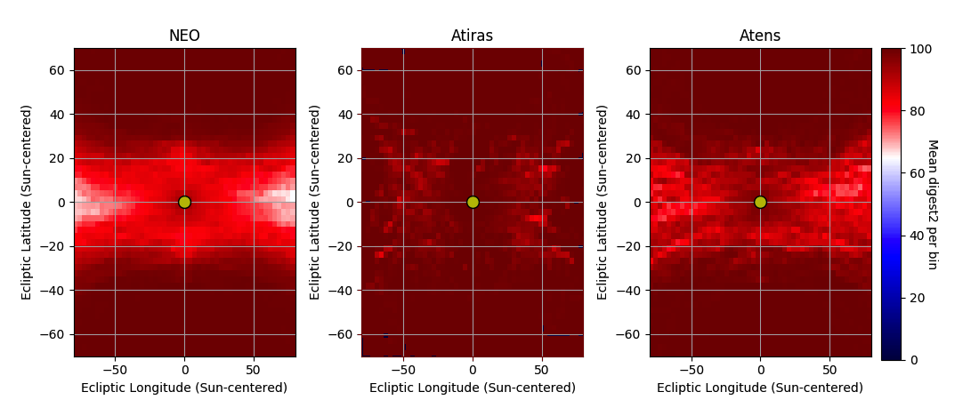
Most of our analyses were focused on NEOs observed in favorable locations of the sky within 100 degrees of the opposition (e.g. Figure 9). In Section IV.2.4 we identified regions near the ecliptic roughly 100 to 60 degrees from the opposition where the mean digest2 score is relatively low. However, some orbit types, such as Atens or Atiras, rarely or never cross the opposition region. Searches close to the Sun are required to find these objects. Ground-based observations near the Sun are limited by large airmass and associated target brightness losses, as well as limited observing time at dawn or dusk. Low Solar elongation observations are ideal for space-based observatories. Figure 15 shows the mean digest2 score for the $Sim$ data set in the Sun-centered ecliptic coordinates. Interestingly, closer to the Sun digest2 is almost always above 65 and Atiras have particularly very large $D_{2}{}$ values. We demonstrated that $\emph{digest2}{}$ score can identify NEOs in low-solar elongations.

IV.7 Interstellar Objects and digest2

The interstellar object (ISO) 1I/’Oumuamua (Bacci et al. 2017) was discovered by the Pan-STARRS NEO survey and its first tracklet was reported to the NEOCP as a $D_{2}{}=100$ tracklet. Subsequent follow-up quickly revealed its hyperbolic orbit. However, without a large NEO $\emph{digest2}{}$ score, it would never have appeared on the NEOCP or been followed-up. As mentioned earlier, one of the key constraints of digest2 are orbits bound to the Sun. Previous work (Engelhardt et al. 2017) showed that the NEO digest2 score could be used to identify ISOs, demonstrating that 2/3 of ISOs in a simulated Pan-STARRS survey achieved $D_{2}{}>90$ at some time while visible.

Figure 16 shows the $D_{2}{}$ , rate of motion and magnitude of all reported 1I/’Oumuamua tracklets. From the time of discovery to November 12, 2017, 1I/’Oumuamua had $D_{2}{}=100$ at all times, and in addition, 1I/’Oumuamua had $D_{2}{}=100$ for the entire time it was visible to the main NEO surveys ( $V\lower 3.01385pt\hbox{$\;\stackrel{{\scriptstyle\textstyle<}}{{\sim}}\;$}22$ ).

V Discussion

We have described the algorithm underlying the digest2 code, as well as its usage to calculate the score of a short-arc tracklet with respect to a given orbit class. We focused on the NEO digest2 score, $D_{2}{}$ , as used by the Minor Planet Center (MPC) to classify the likelihood that submitted sets of detections are NEOs. We showed that $D_{2}{}$ changes for each object as it moves across the sky and its brightness and rate of motion vary. For NEOs, the maximum $D_{2}{}$ reaches the extreme value of $D_{2}{}=100$ for more than 93% of NEOs, and over $99\%$ of NEOs have $D_{2,crit}>65$ at some point while visible. Thus, the vast majority of NEOs have sufficiently high $D_{2}{}$ to allow them to be posted to the NEOCP and be rapidly followed-up by observers around the world.

While the digest2 code identifies short-arc NEOs correctly in the vast majority of cases, there are a small number of cases when $D_{2}{}$ is below the critical threshold, currently set to $D_{2,crit}>65$ . We identify the two locations on the sky, on the ecliptic and at low solar elongations, where the mean $D_{2}{}$ is significantly lower than elsewhere on the sky. This is due to the observing geometry and rates of motion of the objects, that cause them to be confused with Main-Belt objects.

We also demonstrate that without the "repeatable" parameter the digest2 code can generate varying output for the same tracklet due to its random selection of variant orbits. However, the variation in $D_{2}{}$ is small and does not affect scores near extremes ( $D_{2}{}=0$ and $D_{2}{}=100$ ). The MPC uses digest2 without the "repeatable" parameter to avoid bias.

V.1 Future directions

As we move into an era of large surveys that can obtain huge volumes of high-precision observations and utilize highly-precise stellar catalogues, it is clear that the digest2 code must evolve. Future developments to the code will include:

•

It will be possible to characterize observational uncertainties on a per-observation basis, as provided for in the ADES format¹⁸¹⁸ 18 https://minorplanetcenter.net/iau/info/ADES.html.
•

A python wrapper and API to provide simplified usage.
•

A new NEO population model, such as the high-fidelity Granvik et al. 2018 model, will be required. Catalog of known orbits used for unknown population reduction would be generated more frequently.
•

The discrete population bins (in $q,e,i,H$ ) need to be replaced with a smooth 4-dimensional function, perhaps also incorporating additional orbital elements to allow improved discrimination of (e.g.) Hildas and Jupiter Trojans.
•

Replacing the synthetic two-detection approach with a robust statistical treatment of all submitted detections, allowing for a significantly improved handling of NEOs that exhibit non-linear motion during close-approach.
•

Further tests and improvements of the code are needed for space-based NEO surveys, such the proposed NEOCam mission (Mainzer et al. 2015).
•

Replacing the $astorb$ known orbit catalog and its orbit quality metric (Muinonen & Bowell 1993) with the MPC’s orbit catalog¹⁹¹⁹ 19 https://minorplanetcenter.net/iau/MPCORB.html and orbit uncertainty parameter²⁰²⁰ 20 https://minorplanetcenter.net/iau/info/UValue.html.

We emphasize that digest2 constitutes an evolving code-base and that we welcome reports from the community of any bugs found, or of suggestions for future directions²¹²¹ 21 At the time of submission, the digest2 team are currently diagnosing the cause of a rare output-formatting error that appears to afflict approximately 1 in every 50,000 evaluation attempts when running digest2 in a multi-core environment. We anticipate that the solution of this issue will lead to a future version release..

We are grateful to Rob McNaught for his insights regarding the history of the Panglosscode, and for his many clarifications regarding the historical development of ranging. MJH and MJP gratefully acknowledge NASA grants NNX12AE89G, NNX16AD69G, and NNX17AG87G, as well as support from the Smithsonian 2015-2017 Scholarly Studies programs. DJA acknowledges the N. Ireland Dept. for Communities support at Armagh. We are saddened to report that during the course of the work on this manuscript, lead author Sonia Keys died on 13 August 2018 at the age of 57, after a long struggle with cancer. Sonia worked as a commercial software developer from 1983 to 2001 and then began working with the Astronomical Society of Kansas City, specializing in the tracking of Near-Earth Objects (NEOs). Her skill and reliability with NEO astrometry caught the attention of the Minor Planet Center (MPC), and that led to a position as an astronomer and software developer for the MPC. During her tenure at the MPC, Sonia was the lead developer of the digest2 software and was the point-of-contact for the many people in the NEO community that utilized it for over a decade. We deeply regret Sonia’s passing, and we hope that we have completed this manuscript in a manner she would have approved of. We hope this publication and note will serve as a small token of the esteem in which we held her. Sonia was the conscience of the MPC. Her clarity of thought, her willingness to ask difficult questions, and her tenacity will be sorely missed.

Appendix A Variant Orbits

In the following algorithmic description, all line references relate to Algorithm 1 of Section III.

The input file for the digest2 program contains astrometry of short-arc tracklets, such as those illustrated in Appendix F. The file can contain one or many tracklets (Line 1). After the input data are loaded, binned population model is loaded into memory as well (Line 1, Section III.3). Each tracklet is subsequently treated individually (Line 1):

Two observations of an arc are insufficient for a determination of its orbit, or when the observation arc is too short. However, even very short arcs with few observations can be used to derive a range of possible orbits and assess the probability of the asteroid being in a certain region of the Solar system. Because each tracklet has two or more detections (N), as described in Section III.1, two detections either selected ( $N=2$ ) or generated ( $N>2$ ).

The two observables, or detections, $A_{1}$ and $A_{2}$ of the same object (Line 1), are defined by $A_{t_{i}}$ =[ $\alpha_{i},\delta_{i},V_{i}$ ], where $\alpha_{i}$ is the right ascension, $\delta_{i}$ the declination, $V_{i}$ is the apparent magnitude at the time of observation $t_{i}$ .

Because the tracklet consists of $N\geq 2$ data points with unique photometry, either due to photometric errors or rotation of the object, the mean tracklet magnitude $V_{1}$ is computed (line 1) in the Johnson-Cousins V-band photometric system. The transformation to V-band is simple (Vereš et al. 2018), the correction is $-0.8$ if the reported band was $B$ , or $+0.4$ for other bands, except of $V$ , where no correction is applied. If no photometry is provided, $V_{1}=21$ is assumed as a typical magnitude limit of the current asteroid surveys.

We can easily transform the observation [ $\alpha_{i},\delta_{i}$ ] to its topocentric cartesian unit vector (Figure 17) $\vec{d_{i}}=[x_{i},y_{i},z_{i}]$ :

(x_{i},y_{i},z_{i})=(\cos{\alpha_{i}}\cos{\delta_{i}},\,\,\,\sin{\alpha_{i}}\cos{\delta_{i}},\,\,\,\sin{\delta_{i}})

(A1)

For further analysis, we will need to transform unit vectors from equatorial to ecliptic coordinate system (See Figure 17):

\vec{d_{i}}=R_{\epsilon}^{T}\cdot\vec{d_{i}}

(A2)

where $R_{\epsilon}$ is the rotation matrix defined by obliquity of the ecliptic $\epsilon$ :

R_{\epsilon}=\begin{pmatrix}1&0&0\\ 0&\cos{\epsilon}&\sin{\epsilon}\\ 0&-\sin{\epsilon}&\cos{\epsilon}\\ \end{pmatrix}

(A3)

To derive the position state vector $\vec{r}$ , we have to assume a topocentric distance $D$ to the asteroid. In line 1 of Algorithm 1, Sun-observer vectors (labeled $\vec{R_{1}},\vec{R_{2}}$ in Figure 17) in ecliptic Cartesian coordinates are computed by local sidereal time and observer site parallax constants. Observer’s topocentric positions are loaded from MPC-managed list of observatory codes²²²² 22 https://minorplanetcenter.net/iau/info/ObservatoryCodes.html. Also the observer-object unit vectors $\vec{d_{1}},\vec{d_{2}}$ are computed in ecliptic Cartesian coordinates.

Then, the topocentric vector to the first observation, $\vec{\Delta_{1}}$ , will be a scalar multiple of $D$ and the unit vector $\vec{d_{1}}$ . $D$ is one of the values selected recursively (Appendix C) between the minimum (0.05 au) and maximum (100 au) distances within the allowed admissible region:

\vec{\Delta_{1}}=D\,\vec{d_{1}}

(A4)

Knowing the position vectors of the observer with respect to the Sun at the time of the two observations ( $R_{1}$ and $R_{2}$ ) in ecliptic coordinates, we can easily derive the heliocentric state vector $\vec{r_{1}}$ as:

\vec{r_{1}}=\vec{R_{1}}+\vec{\Delta_{1}}

(A5)

After the position vectors are derived, the algorithm continues in investigation of the velocity vectors. The observed motion of the asteroid on the celestial sphere is a projection of the actual velocity vector to the tangent plane. While we do not know the angle between the tangent plane and the velocity vector $\vec{v_{1}}$ , we can make progress by computing the possible ranges of angles (Figure 17 - bottom) under the assumption that the object is bound to the Sun. At a given distance from the Sun, $r_{1}$ , an orbit is bound if its specific orbital energy $\epsilon<0$ . We will find the angles of the $\vec{v_{1}}$ for the parabolic orbits from:

\epsilon=\frac{v_{1}^{2}}{2}-\frac{U}{r_{1}}=0

(A6)

where $U=k^{2}$ is the Gaussian gravitational constant squared²³²³ 23 $k=0.01720209895\,au^{3/2}\,day^{-1}\,(solar\,mass)^{-1/2}$ .

To find $\vec{v_{1}}$ one has to solve triangle $E_{2},A_{1},A_{2}$ on figure 17. The velocity vector will be derived as $\vec{v_{1}}=(\vec{\Delta_{2}}-\vec{\Delta_{21}})/(t_{2}-t_{1})$ .

The angle $\theta$ (Figure 17 - bottom) can be derived by computing the intermediate vector $\vec{\Delta_{21}}$ from vector difference of $\vec{r_{1}}$ and $\vec{R_{2}}$ and the dot product of known unit vector $\vec{d_{2}}$ and derived $\vec{\Delta_{21}}$ :

\displaystyle\begin{split}\vec{\Delta_{21}}=\vec{r_{1}}-\vec{R_{2}}\\ \cos{\theta}=\frac{\vec{\Delta_{21}}\cdot\vec{d_{2}}}{{|\Delta_{21}||1|}}\end{split}

(A7)

Then, by using the cosine rule, substituting $v_{1}=s_{1}/(t_{2}-t_{1})$ and using equation (A6), we can derive the length of the vector $\Delta_{2}$ as follows. Line 1 of Algorithm 1 involves solving a quadratic that gives two values for $\alpha$ corresponding to state vectors $\vec{s}$ and $\vec{s^{*}}$ that represent parabolic orbits:

\displaystyle\begin{split}{\Delta_{21}}^{2}+{\Delta_{2}}^{2}-{s_{1}}^{2}-2{{\Delta_{21}}\Delta_{2}}\cos{\theta}=0\\ {\Delta_{2}^{2}}-2{{\Delta_{2}}{\Delta_{21}}}\cos{\theta}+\left({\Delta_{21}}^{2}-2\frac{U{(t_{2}-t_{1})}^{2}}{{r_{1}}}\right)=0\end{split}

(A8)

Equation (A8) has two roots for $\Delta_{2}$ after doing simple substitution (A, B, C) solving:

\displaystyle\begin{split}(A,B,C)&=(1,\,\,\,-2\Delta_{2}\cos{\theta},\,\,\,{\Delta_{21}}^{2}-2\frac{U{(t_{2}-t_{1})}^{2}}{{r_{1}}})\\ \Delta_{2}&=\frac{-B\pm\sqrt{B^{2}-4AC}}{2A}\end{split}

(A9)

Two roots of $\Delta_{2}$ lead to the extreme solutions of angles at which the vector ${v_{1}}$ of an asteroid is equal to escape velocity:

Based on figure 17 and cosine rules and law of sines:

\displaystyle\begin{split}s_{1}&=\sqrt{\Delta_{2}^{2}+\Delta_{21}^{2}-2\Delta_{21}\Delta_{2}\cos{\theta}}\\ \cos{\alpha}&=\frac{{s_{1}}^{2}+{\Delta_{21}}^{2}-{\Delta_{2}}^{2}}{2{s_{1}}{\Delta_{21}}}\\ \sin{\alpha}&=\frac{{\Delta_{2}}\sin{\theta}}{{s_{1}}}\\ \alpha&=\arctan{\left(\frac{\sin{\alpha}}{\cos{\alpha}}\right)}\end{split}

(A10)

Having the topocentric ( $\vec{r_{1}}$ ) and heliocentric ( $\vec{\Delta_{1}}$ ) distance, the mean V-band magnitude $V_{1}$ and geometry ( $\alpha$ ), we are now able to compute the object’s absolute magnitude $H$ (Line 1) of Algorithm 1 by equation:

H=V_{1}-5\log(\Delta_{1}r_{1})+f(\Phi_{1},G)

(A11)

where the phase angle $\Phi_{1}$ is the angle between $\vec{\Delta_{1}}$ and $\vec{r_{1}}$ and $G$ is the slope parameter. The form of the phase function $f(\Phi,G)$ is based on Bowell et al. 1989 and $G=0.15$ is assumed.

In the next step (Line 1) of Algorithm 1, the algorithm picks angles randomly for a selected topocentric distance $D$ in a range between the two extremes of $\alpha$ that represent a bound elliptical orbit.

With any valid $\alpha$ and $D$ , we can derive the velocity vector, again by using the rule of sines (Figure 17 - bottom):

\displaystyle\begin{split}\Delta_{2}=\frac{\Delta_{21}\sin{\alpha}}{\sin{(\pi-\alpha-\theta)}}\end{split}

(A12)

The heliocentric velocity vector $\vec{v}$ in ecliptic coordinates is

\vec{v}=\frac{{\Delta_{2}}\vec{d_{2}}-\vec{\Delta_{21}}}{t_{2}-t_{1}}

(A13)

Having $\vec{r_{1}}$ , $\vec{v}$ at a given epoch, we have the orbit defined through its state vector (Line 1 of Algorithm 1) which is easy to convert into a set of Keplerian elements (Line 1 of Algorithm 1).

The entire procedure is repeated for a range of assumed distances, $D_{j}$ that lead to set of unique position vectors, $\vec{r_{j}}$ , and velocity vectors, $\vec{v_{j}}$ . Example of variant orbits generated by digest2 in a phase space of $\alpha$ and $\Delta_{1}$ is shown in Figure 18.

Appendix B digest2 Software

B.1 Detailed Historical Evolution

In Section II.1 we provided a brief outline of the historical development of the digest2 algorithm. In Table 5 of this appendix, we provide the interested reader with a more detailed, chronologically-ordered description of the key changes made to the digest2 code.

Table 5: Significant Changes and Versions of Digest2. Archived (and operational) code for the majority of the versions listed in this table are available in https://bitbucket.org/mpcdev/digest2/src/master/archive/.

Date	Version	Description
pre-2002	0.0223	Original FORTRAN 77 code (“223.f”) built on Pangloss
Aug 2005	0.1	MIT-style license, catalog-reduced model.
Sep 2005	0.2	Bin search algorithm (App. C)
Feb 2010	0.3	Pan-STARRS S3M model, multiple orbit classes, improved scoring (§ III.3). Parallelized across multiple CPU cores.
Feb 2010	0.4	Supported space-based observations.
Feb 2010	0.5	Great circle RMS output. Stand-alone GCR utility.
Mar 2010	0.6	Improved stand-alone GCR utility.
Nov 2010	0.7	Orbit classes H18, H22, bug fixes.
Apr 2011	0.8	More flexible output, new config options. Removed stand-alone GCR utility, bug fixes.
Apr 2011	0.9	Bug fixes.
Apr 2011	0.10	Bug fixes.
May 2011	0.11	Endpoint synthesis (§ III.1). Observational Error (§ IV.4.2).
May 2012	0.12	Bug fixes.
Jun 2012	0.13	Bug fixes.
Jan 2013	0.14	Bug fixes.
Feb 2014	0.15	Allow more obscodes.
Feb 2015	0.16	Command line option to limit parallelism.
Jun 2015	0.17	CSV model, bug fixes.
Jun 2015	0.18	Minor usability improvements. Bug fixes.
Aug 2017	0.19	Bug fixes, including a serious uninitialized data problem.

B.2 Software Availability and Usage

The digest2 source code and the documentation is freely available at https://bitbucket.org/mpcdev/digest2/overview. The download section contains a zip archive of digest2 and the population model tar achive d2model.

The synthetic solar system model binning and reduction source code MUK is freely available at https://bitbucket.org/mpcdev/d2model/src/master/muk.c.

The digest2 code can be executed directly after its compilation using the supplied input observation file (sample.obs) and configuration file (MPC.config) as follows:

digest2 -c MPC.config sample.obs

Further detailed instructions for the operation of digest2 can be found in https://bitbucket.org/mpcdev/digest2/src/master/OPERATION.md.

Appendix C Binary Search Algorithm for Population Bins

The initial algorithm (version 0.1) for constructing class scores was as in Algorithm 2.

…

for distance $D\leftarrow$ .025 AU to 7 by .025 do

for $\alpha\leftarrow\alpha_{1}$ to $\alpha_{2}$ by $2\arcdeg$ do

Look-up

BinPopn(a,e,i,H)

if $Interesting(a,e,i)$ then

neo\mathrel{+}=BinPopn

else

mb\mathrel{+}=BinPopn

score

\leftarrow 100*neo/(neo+mb)

Algorithm 2 digest2 scoring version 0.1

On line 2 the function $Interesting$ tests if candidate elements are in the class of interest. The single class of interest defined in digest2 versions-0.1 and -0.2 corresponded to the Minor Planet Center’s definition of “interesting” which included not just NEOs ( $q<1.3$ ) but also high eccentricity ( $e>0.5$ ) and high inclination ( $i>40$ ) orbits which would also lead to a discovery MPEC. The current code uses the classes described in Table 8 of Appendix D.

Version-0.2 contained an improved score formula. The goal of the new score formula was to change the computation of the variables neo and mb (Algorithm 2 lines 2 and 2) to be more like,

	$\displaystyle neo$	$\displaystyle=\text{ sum of bin populations over all represented NEO bins}$		(C1)
	$\displaystyle mb$	$\displaystyle=\text{ sum of bin populations over all represented non-NEO bins},$		(C1)

where a best effort is made to locate all the population bins represented by the input arc. The reasons for this change ultimately stem from a desire to (a) avoid double-counting population bins, and (b) avoid omitting population bins due to the use of overly large distance and/or angle step-sizes in Algorithm 2.

Per-class binning enables enhancements to the bin tagging and scoring algorithms. In the current version of digest2, separate bin tags are accumulated per class. Further, for each class, two sets of tags are accumulated per class. An in-class tag is set for a bin when a candidate orbit meets the class definition. A separate out-of-class tag is set otherwise. Two population sums are then computed for each class, a sum of bin populations with in-class tags and sum of bin populations with out-of-class tags. The first represents the sum of class bin populations where a candidate orbit of class was found. The second represents the sum of out-of-class bin populations where a candidate orbit out of class was found.

Computations at a single distance follow algorithm 1 steps 1 through 1, but then call a recursive function to subdivide the angle space between $\alpha_{1}$ and $\alpha_{2}$ .

At each call, a state vector and then orbital elements are computed, but then rather than accessing the indicated bin population, the corresponding tag is simply checked (in the distance-specific tags). If the tag was already set, subdivision ends and the recursive function returns. If the tag was not set, then the angle space is subdivided further and the recursive function is called for each subdivision.

The distance, $D$ , is subdivided similarly with a separate recursive function. On each call, computations are performed for a single distance as just described, then the distance-specific tags are checked. If all bins tagged at that distance had previously been tagged in the overall result, the recursive function simply returns. If new bins were tagged, they are merged into the overall result, the distance space is subdivided further, and the recursive (distance) function is called for each subdivision. After all subdivision functions return, the formulas above for $neo$ and $mb$ are computed as described in Algorithm 3.

for each tag of overall tags do

if tag set then

if interesting bin then

neo\leftarrow neo+BinPop(a,e,i,H)

if non-interesting bin then

mb\leftarrow mb+BinPop(a,e,i,H)

Algorithm 3 Tag accumulation

Appendix D Tabulated Values and Settings for digest2

In Table 6 we list the assumed astrometric uncertainties adopted in the latest version of the digest2 code. The values are set in the file MPC.config and can be altered by the user.

Table 6: Astrometric uncertainties currently used by digest2 by the MPC and digest2 code, based on long-term statistics²⁵²⁵ 25 https://minorplanetcenter.net/iau/special/residuals.txt.

observatory	astrometric	observatory	astrometric
code	uncertainty	code	uncertainty
106	0.4"	D29	0.5"
291	0.4"	E12	0.5"
568	0.1"	F51	0.2"
691	0.4"	F52	0.2"
703	0.7"	G96	0.3"
704	0.7"	H15	0.5"
A50	0.5"	J75	0.4"
C51	0.7	other	1.0"

digest2 is configurable with keywords that allow control of the output and setup of some input variables. The keywords are set in the same file (MPC.config) as the astrometric uncertainties (Table 6). The available keywords are described in Table 7.

Table 7: Keywords available in digest2.

keyword	meaning
headings	show heading
noheadings	hide heading
rms	show residual RMS from linear motion along a great circle in arc-seconds
norms	do not show RMS
raw	show raw digest2 (Section III.3.1)
noid	show noid digest2 (Section III.3.2)
repeatable	random seed is defined and always the same (Section IV.4.1)
random	pseudo-random generation of $\alpha$ and resulting digest2 (Section IV.4.1)
obserr	fixed astrometric uncertainty set to a value in arc seconds
poss	show other non-zero resulting scores in addition to specified classes digest2
any orbit class(es) defined in Table 8	e.g. NEO
user defined astrometric uncertainty (arc seconds) per MPC observatory code	e.g. obserrF51=0.2
default keywords: noid, rms, headings, N22, N18, NEO, Int, obserr=1.0

The orbit classes used by digest2 are defined by the orbital elements and absolute magnitudes listed in Table 8.

Table 8: Definitions of orbital classes in digest2.

orbit class	abbreviation	definition in keplerian elements and absolute magnitude
MPC Interesting	Int	q < 1.3 \|\| e >= 0.5 \|\| i >= 40 \|\| Q > 10
Near-Earth Object	NEO	q < 1.3
Large Near-Earth Object	N18	q < 1.3 & H<18.5
Intermediate-size Near-Earth Objects	N22	q < 1.3 & H<22.5
Mars-Crossers	MC	q < 1.67 & q >= 1.3 & Q > 1.58
Hungarias	Hun	a < 2 & a > 1.78 & e < 0.18 & i > 16 & i < 34
Phocaeas	Pho	a < 2.45 & a > 2.2 & q > 1.5 & i > 20 & i < 27
Inner Main Belt	MB1	q > 1.67 & a < 2.5 & a > 2.1 & i < ((a - 2.1) / 0.4) * 10 + 7
Pallas family	Pal	a < 2.8 & a > 2.5 & e < 0.35 & i > 24 & i < 37
Hansas	Han	a < 2.72 & a > 2.55 & e < 0.25 & i > 20 & i < 23.5
Central Main Belt	MB2	a < 2.8 & a > 2.5 & e < 0.45 & i < 20
Outer Main Belt	MB3	e < 0.4 & a > 2.8 & a < 3.25 & i < ((a - 2.8) / 0.45) * 16 + 20
Hildas	Hil	a > 3.9 & a < 4.02 & i < 18 & e < 0.4
Jupiter Trojans	JTr	a > 5.05 & a < 5.35 & e < 0.22 & i < 38
Jupiter Family Comets	JFC	q > 1.3 & $T_{J}>2$ & $T_{J}<3$
$T_{J}$ - Tisserand parameter with respect to Jupiter, a - semimajor axis (AU), e - eccentricity, i - inclination (deg)
Q - aphelion distance (AU), q - perihelion distance (AU), H - absolute magnitude

Appendix E Population bins

In Figure 19 we illustrate the population model used by digest2 (see Section III.3 above for further description).

Appendix F Example Tracklet

We provide an example of a tracklet taken from a a typical Hungaria-group asteroid. The data is presented in a standardized 80-column format²⁶²⁶ 26 https://minorplanetcenter.net/iau/info/ObsFormat.html - Minor Planet Packed Designation (K18B01E), Mode of Observation ("C" for CCD), Time of observations (Year, Month, Day), Right Ascension (Hours, Minutes, Seconds) and Declination (Degrees, Minutes, Seconds), Magnitude, Band ("w"), Catalog Code ("U"), Packed Reference (" $\sim$ 2VXl") and Observatory Code ("F51").

     K18B01E* C2018 01 17.42780 08 01 58.347+41 29 48.20         21.4 wU~2VXlF51
     K18B01E  C2018 01 17.43919 08 01 57.028+41 29 44.58         21.2 wU~2VXlF51
     K18B01E  C2018 01 17.46196 08 01 54.365+41 29 37.55         21.2 wU~2VXlF51

References

Bacci et al. (2017) Bacci, P., Maestripieri, M., Tesi, L., et al. 2017, Minor Planet Electronic Circulars, 2017
Boattini et al. (2007) Boattini, A., Milani, A., Gronchi, G. F., Spahr, T., & Valsecchi, G. B. 2007, in IAU Symposium, Vol. 236, Near Earth Objects, our Celestial Neighbors: Opportunity and Risk, ed. G. B. Valsecchi, D. Vokrouhlický, & A. Milani, 291–300
Bolin et al. (2014) Bolin, B., Jedicke, R., Granvik, M., et al. 2014, Icarus, 241, 280, doi: 10.1016/j.icarus.2014.05.026
Bowell (1989) Bowell, E. 1989, in BAAS, Vol. 21, Bulletin of the American Astronomical Society, 969
Bowell (2018) Bowell, E. 2018, The Asteroid Orbital Elements Database. ftp://ftp.lowell.edu/pub/elgb/astorb.html
Bowell et al. (1989) Bowell, E., Hapke, B., Domingue, D., et al. 1989, in Asteroids II, ed. R. P. Binzel, T. Gehrels, & M. S. Matthews, 524–556
Bowell et al. (1994) Bowell, E., Muinonen, K., & Wasserman, L. H. 1994, in IAU Symposium, Vol. 160, Asteroids, Comets, Meteors 1993, ed. A. Milani, M. di Martino, & A. Cellino, 477–481
Bowell et al. (1990) Bowell, E., Skiff, B. A., & Wasserman, L. H. 1990, in Asteroids, Comets, Meteors III, ed. C. I. Lagerkvist, H. Rickman, & B. A. Lindblad, 19
Chesley (2005) Chesley, S. R. 2005, in IAU Colloq. 197: Dynamics of Populations of Planetary Systems, ed. Z. Knežević & A. Milani, 255–258
Chesley & Spahr (2004) Chesley, S. R., & Spahr, T. B. 2004, in Mitigation of Hazardous Comets and Asteroids, ed. M. J. S. Belton, T. H. Morgan, N. H. Samarasinha, & D. K. Yeomans, 22
Connors et al. (2011) Connors, M., Wiegert, P., & Veillet, C. 2011, Nature, 475, 481, doi: 10.1038/nature10233
de la Fuente Marcos & de la Fuente Marcos (2016) de la Fuente Marcos, C., & de la Fuente Marcos, R. 2016, MNRAS, 462, 3441, doi: 10.1093/mnras/stw1972
Engelhardt et al. (2017) Engelhardt, T., Jedicke, R., Vereš, P., et al. 2017, AJ, 153, 133, doi: 10.3847/1538-3881/aa5c8a
Farnocchia et al. (2015) Farnocchia, D., Chesley, S. R., & Micheli, M. 2015, Icarus, 258, 18, doi: 10.1016/j.icarus.2015.05.032
Granvik et al. (2012) Granvik, M., Vaubaillon, J., & Jedicke, R. 2012, Icarus, 218, 262, doi: 10.1016/j.icarus.2011.12.003
Granvik et al. (2018) Granvik, M., Morbidelli, A., Jedicke, R., et al. 2018, Icarus, 312, 181, doi: 10.1016/j.icarus.2018.04.018
Grav et al. (2011) Grav, T., Jedicke, R., Denneau, L., et al. 2011, PASP, 123, 423, doi: 10.1086/659833
Jedicke (1996) Jedicke, R. 1996, AJ, 111, 970, doi: 10.1086/117844
Kubica et al. (2007) Kubica, J., Denneau, L., Grav, T., et al. 2007, Icarus, 189, 151, doi: 10.1016/j.icarus.2007.01.008
Mainzer et al. (2015) Mainzer, A., Grav, T., Bauer, J., et al. 2015, AJ, 149, 172, doi: 10.1088/0004-6256/149/5/172
Mainzer et al. (2012) Mainzer, A., Grav, T., Masiero, J., et al. 2012, ApJ, 760, L12, doi: 10.1088/2041-8205/760/1/L12
Marsden (1985) Marsden, B. G. 1985, AJ, 90, 1541, doi: 10.1086/113867
Marsden (1991) —. 1991, AJ, 102, 1539, doi: 10.1086/115979
McNaught (1999) McNaught, R. 1999, Journal of the British Astronomical Association, 109, 294
Milani et al. (2004) Milani, A., Gronchi, G. F., Vitturi, M. D., & Knežević, Z. 2004, Celestial Mechanics and Dynamical Astronomy, 90, 57, doi: 10.1007/s10569-004-6593-5
Milani & Knežević (2005) Milani, A., & Knežević, Z. 2005, Celestial Mechanics and Dynamical Astronomy, 92, 1, doi: 10.1007/s10569-005-3314-7
Morrison (1992) Morrison, D., ed. 1992, The Spaceguard survey
Muinonen & Bowell (1993) Muinonen, K., & Bowell, E. 1993, Icarus, 104, 255, doi: 10.1006/icar.1993.1100
Oszkiewicz et al. (2009) Oszkiewicz, D., Muinonen, K., Virtanen, J., & Granvik, M. 2009, Meteoritics and Planetary Science, 44, 1897, doi: 10.1111/j.1945-5100.2009.tb01999.x
Spoto et al. (2018) Spoto, F., Del Vigna, A., Milani, A., et al. 2018, ArXiv e-prints. https://arxiv.org/abs/1801.04004
Stokes & Yeomans (2003) Stokes, G. H., & Yeomans, D. K. 2003, AGU Fall Meeting Abstracts, P51E
Tholen & Whiteley (2000) Tholen, D. J., & Whiteley, R. J. 2000, in Bulletin of the American Astronomical Society, Vol. 32, AAS/Division for Planetary Sciences Meeting Abstracts #32, 1018
Väisälä (1939) Väisälä, Y. 1939, Ann. Acad. Sci. Fenn. A : Astron.-Optika Inst. Univ. Turku Informo No. 1., 52, 2
Vereš & Chesley (2017) Vereš, P., & Chesley, S. R. 2017, AJ, 154, 12, doi: 10.3847/1538-3881/aa73d1
Vereš et al. (2018) Vereš, P., Payne, M. J., Holman, M. J., et al. 2018, AJ, 156, 5, doi: 10.3847/1538-3881/aac37d
Virtanen et al. (2001) Virtanen, J., Muinonen, K., & Bowell, E. 2001, Icarus, 154, 412, doi: 10.1006/icar.2001.6592

The digest2 NEO Classification CodeJournal: PASP, Day Month Year

Abstract

Keywords:

I Introduction

II Methodology

II.1 Historical Development of digest2

III Computational elements of digest2

III.1 Endpoint Synthesis

III.1.1 Dithering and Observational Uncertainty

III.2 Orbit Solution

III.3 Population Model used by digest2

III.3.1 Full Population Model

III.3.2 Unknown Population

III.4 Searching for bins

III.5 Class Score

III.6 Algorithmic Summary

IV digest2 score analysis

IV.1 Application of digest2 to Individual Objects

IV.2 Application of digest2 to Populations

IV.2.1 Data Sets and Simulations

IV.2.2 Distribution of digest2 Scores

IV.2.3 Comparison of NEO digest2 Scores Across Data Sets

IV.2.4 Detailed Analysis of digest2 scores for NEOs

IV.3 Accuracy, Precision and the NEOCP

IV.4 Nuances of Practical digest2 Usage

IV.4.1 Effects of Random-Choice of α\alpha

IV.4.2 Effects of Observational Uncertainty

IV.4.3 Great Circle Departure

IV.5 Earth quasi-satellites, co-orbitals and Trojans

IV.6 NEOs at low Solar elongations

IV.7 Interstellar Objects and digest2

V Discussion

V.1 Future directions

Appendix A Variant Orbits

Appendix B digest2 Software

B.1 Detailed Historical Evolution

B.2 Software Availability and Usage

Appendix C Binary Search Algorithm for Population Bins

Appendix D Tabulated Values and Settings for digest2

Appendix E Population bins

Appendix F Example Tracklet

References

IV.4.1 Effects of Random-Choice of $\alpha$