Disagreement-based Active Learning in
Online SettingsThanks: This work was supported by the National Science Foundation under Grant CCF-1815559.

The above problem falls under the general framework of active learning. In contrast to passive learning where labeled examples are given a priori or drawn at random, active learning asserts control over which labeled examples to learn from by actively querying the labels for carefully selected instances. The hope is that by learning from the most informative examples, the same level of classification accuracy can be achieved with much fewer labels than in passive learning.

We consider a general instance space $\mathcal{X}$, a general hypothesis space $\mathcal{H}$ of Vapnik-Chervonenkis (VC) dimension $d$ , and the Tsybakov noise model parameterized by $\alpha\in(0,1]$ [28]. We develop an online active learning algorithm and establish its $O(dT^{\frac{2-2\alpha}{2-\alpha}}\log^{2}T)$ label complexity and uniformly bounded regret in prediction errors with respect to the best classifier $h^{*}$ in $\mathcal{H}$. More specifically, the total expected classification errors in excess to $h^{*}$ over a horizon of length $T$ is bounded below $1/2$ independent of $T$, demonstrating that the proposed algorithm offers practically the same level of classification accuracy as $h^{*}$ with a sublinear label complexity in $T$. We further establish a matching (up to a poly-logarithmic factor) lower bound, demonstrating the order optimality of the proposed algorithm. We address the tradeoff between label complexity and regret and show that the algorithm can be modified to operate at a different point on the tradeoff curve. Below we contextualize this work with respect to the existing literature by highlighting the differences in three aspects: algorithm design, analysis techniques, and performance comparison.

Let $\{X_{t}\}_{t\geq 1}$ be a streaming sequence of instances, each drawn from an instance/sample space $\mathcal{X}$ and characterized by its feature vector. Each subset of $\mathcal{X}$ is a concept. There is a target concept $\mathcal{C}\subset\mathcal{X}$ that the learner aims to learn (e.g., learning the concept “table” from household objects). Relating to the target concept $\mathcal{C}$, each instance $X_{t}$ has a hidden label $Y_{t}$, indicating whether $X_{t}\in\mathcal{C}$ (i.e., a positive example wherein $Y_{t}=1$) or $X_{t}\notin\mathcal{C}$ (a negative example with $Y_{t}=0$). The label $Y_{t}$ relates probabilistically to $X_{t}$ according to an unknown conditional distribution $\mathbb{P}_{Y|X}$.

The learner is characterized by its hypothesis space $\mathcal{H}$ consisting of all classifiers under consideration. Each hypothesis $h\in\mathcal{H}$ is a measurable function mapping from $\mathcal{X}$ to $\{0,1\}$. The complexity of the hypothesis space $\mathcal{H}$ is measured by its VC dimension $d$.

Recall that $\mathbb{P}_{Y|X}$ denotes the conditional distribution of the true label $Y$ for a given $X$. Let $\mathbb{P}_{X}$ denote the unknown marginal distribution of instances $X$ and $\mathbb{P}=\mathbb{P}_{X}\times\mathbb{P}_{Y|X}$ the joint distribution of an example $(X,Y)$. The error rate of a hypothesis $h$ is given by

which is the probability that $h$ misclassifies a random instance. Define the pseudo-distance and the disagreement between two hypotheses as, respectively,

where the distance is the difference in error rates and the disagreement is the probability mass of the instances over which the two hypotheses disagree. Lastly, $\mathcal{D}(h_{1},h_{2})=\{x\in\mathcal{X}:h_{1}(x)\neq h_{2}(x)\}$ denotes the disagreement region between two hypotheses $h_{1}$ and $h_{2}$.

Let $h^{*}$ be the Bayes optimal classifier that minimizes the error rate, i.e., for all $x\in\mathcal{X}$, $h^{*}(x)$ is the label that minimizes the probability of classification error:

where $\mathbbm{1}[\cdot]$ is the indicator function. Let

It is easy to see that

We assume that $h^{*}\in\mathcal{H}$.

The function $\eta(x)$ given in (4) is a measure of the feature noise level at $x$. The noise-free case is when labels are deterministic: $\mathbb{P}_{Y|X=x}$, hence $\eta(x)$, assumes only values of $0$ and $1$. In this case, the optimal classifier $h^{*}$ is error-free. This is referred to as the realizable case with perfectly separable data.

In a general agnostic case with arbitrary $\mathbb{P}_{Y|X}$, consistent classifiers may not exist, and even $h^{*}$ suffers a positive error rate. A particular case, referred to as the Massart bounded noise condition [32], is when $\eta(x)$ is discontinuous at the boundary between positive examples $\mathcal{X}^{*}_{1}\triangleq\{x\in\mathcal{X}:h^{*}(x)=1\}$ and negative examples $\mathcal{X}^{*}_{0}\triangleq\{x\in\mathcal{X}:h^{*}(x)=0\}$. Specifically, there exists $\gamma>0$ such that $|\eta(x)-\frac{1}{2}|\geq\gamma$ for all $x\in\mathcal{X}$.

A more general noise model is the Tsybakov noise condition [28], for which the Massart bounded noise condition is a special case. It allows $\eta(x)$ to pass $\frac{1}{2}$ with a continuous change across the decision boundary and parameterizes the slope around the boundary. Specifically, the Tsybakov noise condition states that there exist $\alpha\in(0,1]$, $c_{0}\geq 0$, such that for all $h$, we have

At $\alpha=1$, the Tsybakov noise reduces to the more benign Massart noise. In terms of the slope around the decision boundary, the above condition can be restated as

for some constant $c_{0}^{\prime}\geq 0$.

An online active learning strategy $\pi$ consists of a sequence of query rules $\{\upsilon_{t}\}_{t\geq 1}$ and a sequence of prediction rules $\{\lambda_{t}\}_{t\geq 1}$, where $\upsilon_{t}$ and $\lambda_{t}$ map from causally available information consisting of past actions, instances, and queried labels to, respectively, the query decision of $0$ (no query) or $1$ (query) and a predicted label at time $t$. With a slight abuse of notation, we also let $\upsilon_{t}$ and $\lambda_{t}$ denote the resulting query decision and the predicted label at time $t$ under these respective rules.

The performance of policy $\pi=(\{\upsilon_{t}\},\,\{\lambda_{t}\})$ over a horizon of length $T$ is measured by the expected number of queries and the expected number of classification errors in excess to that of the Bayes optimal classifier $h^{*}$. These two performance measures, referred to as label complexity $\mathbb{E}[Q(T)]$ and regret $\mathbb{E}[R(T)]$, are given as follows.

where the expectation is with respect to the stochastic process induced by $\pi$. Note that regret measures the expected difference in the cumulative classification errors over the entire horizon between a learner employing $\pi$ and an oracle that uses $h^{*}$ all through the horizon.

The objective is a learning algorithm that minimizes the label complexity $\mathbb{E}[Q(T)]$ with a constraint on the regret $\mathbb{E}[R(T)]$. The constraint, for example, can be either bounded by a constant independent of $T$ or in a logarithmic order of $T$.

The algorithm operates under an epoch structure. When a fixed number $M$ of labels have been queried in the current epoch, this epoch ends and the next one starts. Note that the epoch length, lower bounded by $M$, is random due to the real-time active query decisions. The algorithm maintains two sets in each epoch $k$: the version space $\mathcal{H}_{k}$ and the RoD $\mathcal{D}(\mathcal{H}_{k})$ defined as the region of instances for which there is disagreement among hypotheses in the current version space $\mathcal{H}_{k}$. More specifically,

The initial version space is set to the entire hypothesis space $\mathcal{H}$, and the initial RoD is the instance space $\mathcal{X}$. At the end of each epoch, these two sets are updated using the $M$ labels obtained in this epoch, and the algorithm iterates into the next epoch.

At each time instant $t$ of epoch $k$, the query and prediction decisions are as follows. If $x_{t}\in\mathcal{D}(\mathcal{H}_{k})$, its label is queried. Otherwise, the learner predicts the label of $x_{t}$ using an arbitrary hypothesis in $\mathcal{H}_{k}$.

At the end of the epoch, $\mathcal{H}_{k}$ is updated as follows. Let $\mathcal{Z}_{k}$ denote the set of the $M$ queried examples in this epoch. For a hypothesis $h$ in $\mathcal{H}_{k}$, define its empirical error over $\mathcal{Z}_{k}$ as

Let $h^{*}_{k}=\arg\min_{h\in\mathcal{H}_{k}}\epsilon_{\mathcal{Z}_{k}}(h)$ be the best hypothesis in $\mathcal{H}_{k}$ in terms of empirical error over $\mathcal{Z}_{k}$. The version space is then updated by eliminating each hypothesis $h$ whose empirical error over $\mathcal{Z}_{k}$ exceeds that of $h^{*}_{k}$ by a threshold $\Delta_{\mathcal{Z}_{k}}(h,h_{k}^{*})$ that is specific to $h$, $h_{k}^{*}$, and $\mathcal{Z}_{k}$. Specifically,

The new RoD $\mathcal{D}(\mathcal{H}_{k+1})$ is then determined by $\mathcal{H}_{k+1}$ as in (10).

We now discuss the key issue of designing the threshold $\Delta_{\mathcal{Z}_{k}}(h,h_{k}^{*})$ for eliminating suboptimal hypotheses. This elimination threshold controls the tradeoff between two conflicting objectives: quickly shrinking the RoD (thus reducing label complexity) and managing the irreversible risk of eliminating good classifiers (thus increasing future classification errors).

In OLA, we obtain a more aggressive threshold design focusing on empirical errors incurred over significant $(X,Y)$ examples determined by the current RoD.

Specifically, for a pair of hypotheses $h_{1},h_{2}$, define

which is the probability that $h_{1}$ misclassifies a random instance but $h_{2}$ successfully classified. For a finite set $\mathcal{Z}$ of $(x,y)$ samples, the empirical excess error of $h_{1}$ over $h_{2}$ on $\mathcal{Z}$ is defined as

The elimination threshold $\Delta_{\mathcal{Z}_{k}}(h,h_{k}^{*})$ is set to:

where $\beta_{\mathcal{H}^{\prime},n}=\sqrt{(4/n)\ln(16T^{2}\mathcal{S}(\mathcal{H}^{\prime},2n)^{2})}$ for an arbitrary hypothesis space $\mathcal{H}^{\prime}$ and positive integer $n$. Here $\mathcal{S}(\mathcal{H}^{\prime},n)$ is the $n$-th shattering coefficient of $\mathcal{H}^{\prime}$. By Sauer’s lemma [33], $\mathcal{S}(\mathcal{H}^{\prime},n)=O(n^{d^{\prime}})$ with $d^{\prime}$ being the VC dimension of $\mathcal{H}^{\prime}$.

The choice of this specific threshold function will become clear in Sec. IV-A when the relationship between the empirical error difference of two hypotheses and the ensemble error rate difference under $\mathbb{P}$ is analyzed.

A detailed description of the algorithm is given in Algorithm 1. The algorithm parameter $M$ is set to $\lceil mdT^{\frac{2-2\alpha}{2-\alpha}}\log T\rceil$, where $m$ is a positive integer whose value will be discussed in Sec. IV-B. We point out that while the horizon length $T$ is used as an input parameter to the algorithm, the standard doubling trick can be applied when $T$ is unknown.

Next, using Theorem 1 we show that the expected regret of the proposed OLA algorithm is bounded by $1/2$.

For the purpose of label complexity analysis, we define the following online disagreement coefficient, which is slightly different from the disagreement coefficient defined for offline active learning in [5].

Recall the psuedo-metric $\rho$ defined in (2). The online disagreement coefficient $\theta=\theta(\mathbb{P},\mathcal{H})$ is defined as

where $B(h,r)=\{h\in\mathcal{H}:\rho(h,h^{\prime})<r\}$ is a “hypothesis ball” centered at $h$ with radius $r$.

The quantity $\theta$ bounds the rate at which the disagreement mass of the ball $B(h^{*},r)$ grows with the radius $r$. It is bounded by $\sqrt{d}$ when $\mathcal{H}$ is $d$-dimensional homogeneous separators [5].

Next we upper bound the label complexity for the proposed online active learning algorithm.

Note that $m$ is a constant determined by the algorithm, the label complexity $\mathbb{E}[Q(T)]$ has an order of $O(dT^{\frac{2-2\alpha}{2-\alpha}}\log^{2}T)$. For the Massart noise condition at $\alpha=1$, the label complexity is $O(d\log^{2}T)$.

We now establish the order optimality of the label complexity of OLA under a bounded regret constraint. This is obtained by establishing a lower bound on the label complexity feasible under any policy with a bounded regret.

Note that a lower bound on the noise (i.e., an upper bound specified through the constant $c_{2}$ on the slope of $\eta(x)$ passing $1/2$) is further imposed in order to establish a tight lower bound on label complexity for a specific noise level. We point out that while we focused on the constraint of a bounded regret, the analysis can be easily modified to obtain lower bounds under regret constraints of different orders. Specifically, we can show a lower bound of $\Omega\left(\min\{T^{2(1-\alpha)(1-\epsilon)},T^{\frac{2-2\alpha}{2-\alpha}}\}\right)$ under a regret constraint of order $O(T^{\epsilon})$ for some $\epsilon>0$. It is also straightforward to modify the lower bound analysis to accommodate different problem models (e.g., those studied in [26, 27]).

For the case of Massart Noise, we can establish a lower bound of $\Omega(\log T)$ under the constraint of a sublinear regret budget. The basic proof technique follows similar ideas as that for the Tsybakov noise but with a simplified analysis (See Appendix D). We summarize the lower bound for the case of Massart Noise in the following theorem.

For constraints of sublinear but unbounded regret, the above lower bound is tight since it matches with the upper bound on the label complexity of RW-OLA (see Sec. V). Under the constraint of bounded regret, however, we conjecture a $\Omega(\log^{2}T)$ lower bound on label complexity for a general hypothesis space with an infinite number of hypotheses. ²² 2 The intuition behind this conjecture is as follows. Let $N(\epsilon)$ denote the $\epsilon$-covering number of $\mathcal{H}$ and $\mathcal{C}$ be an associated $\epsilon$-cover that has $N(\epsilon)$ hypotheses. Specifically, an $\epsilon$-cover $\mathcal{C}$ of $\mathcal{H}$ is a subset of hypothesis $\{h_{1},\dots,h_{N}\}$ such that for any $h\in\mathcal{H}$ there exists an $i\in\{1,2,\dots,N\}$ such that $\rho(h,h_{i})\leq\epsilon$ and the $\epsilon$-covering number of $\mathcal{H}$ is the size of the smallest $\epsilon$-cover of $\mathcal{H}$. Following the same line of arguments in the proof of Theorem 5, we can show that for a hypothesis $h\in\mathcal{C}$, the policy needs to query $\Omega(\log T)$ instances in $\mathcal{D}(h,h^{*})$ to ensure a bounded regret and this needs to hold simultaneously for all $h\in\mathcal{C}$ by the end of the time horizon. Using the uniformity of the cover $\mathcal{C}$, we can show that the expected number of queries to hit $\Omega(\log T)$ queries in $\mathcal{D}(h,h^{*})$ for all $h\in\mathcal{C}$ is $\Omega(\log T\log N(\epsilon))$. Choosing $\epsilon\sim T^{-1/2}$ results in a bound of $\Omega(\log^{2}T)$ on label complexity.

In this section, we show that OLA can be modified to operate on a different point on the tradeoff curve of regret vs. label complexity.

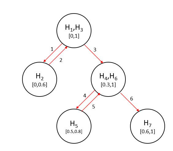
In OLA, the threshold for elimination is constructed conservatively to achieve a bounded regret. More specifically, the outage probability of eliminating $h^{*}$ from the version space (i.e., the parameter $\delta$ in Theorem 1) in each epoch is capped at a small value $1/T^{2}$ that diminishes with $T$. We now consider a variant of OLA in which the elimination probability $\delta$ is set to a constant in order to quickly shrink RoD for a lower label complexity. To mitigate the high probability of $h^{*}$ being eliminated, which may result in a linear regret order, we build in a verification stage at the beginning of each epoch for the algorithm to self recognize and recover from the event of $h^{*}$ being eliminated. The key idea is to devise a biased random walk on the version spaces that allows the algorithm to trace back to a previous version space in the event of $h^{*}$ being eliminated. We refer to this variant of OLA as RW-OLA.

Before delving into the details of the verification stage, we define the parent and child relationship between version spaces. For each epoch $k$, if $\mathcal{H}_{k}$ is obtained by eliminating some of the hypotheses in the version space $\mathcal{H}_{r(k)}$ of a previous epoch $r(k)$, we say that $\mathcal{H}_{r(k)}$ is the parent of $\mathcal{H}_{k}$ and $\mathcal{H}_{k}$ is a child of $\mathcal{H}_{r(k)}$. Note that $\mathcal{H}_{k}$ is a subset of $\mathcal{H}_{r(k)}$.

There are several steps in OLA and RW-OLA that can be computational expensive, which is inherent to the disagreement-based approach. Specifically, maintaining the version space and RoD, and computing the best empirical hypothesis $h^{*}_{k}$ can be costly. We discuss here approximate implementations with manageable computational complexity for homogeneous linear classification, drawing inspiration from techniques of using surrogate loss [13] and the Query-by-Committee approaches [35, 14].

In homogeneous linear classification, $\mathcal{X}$ is the surface of the $d$-dimension unit Euclidean sphere. Each hypothesis, as a linear separator that passes the origin, is given by a unit vector $\mathbf{u}\in\mathbb{R}^{d}$ such that the corresponding concept is $\{\mathbf{x}\in\mathcal{X}:\mathbf{u}\mathbf{x}\geq 0\}$.

To estimate the best empirical hypothesis $h^{*}_{k}$, we use hinge loss function $l(z)=\max\{1-z,0\}$ to replace the 0-1 loss function in (11). Then, the best empirical hypothesis $\hat{h}^{*}_{k}$ under hinge loss is given by

Then standard linear classification algorithms such as SVM can be employed to compute $\hat{h}^{*}_{k}$.

The version space is approximated with $N$ constituent hypotheses sampled uniformly at random. Specifically, at $t=1$, we sample $N$ hypotheses uniformly at random from the entire hypothesis space $\{\mathbf{u}\in\mathbb{R}^{d},||\mathbf{u}||=1\}$ and form $\hat{\mathcal{H}_{1}}$. At each epoch $k$, for each hypothesis $h\in\hat{\mathcal{H}}_{k}$, we check whether it should be eliminated based on (12) and label them as +1 or -1 accordingly. Then, we run a linear classification algorithm to find a linear classifier $\mathbf{\omega}\mathbf{u}+b\geq 0$ that separates them. To obtain an approximate of the new version space $\hat{\mathcal{H}}_{k+1}$, we again sample $N$ hypotheses uniformly at random from $\{\mathbf{u}:\mathbf{\omega}\mathbf{u}+b\geq 0\}$ to form the next version space $\hat{\mathcal{H}}_{k+1}$.

Since the version space is estimated by a finite number of hypotheses, instead of maintaining the RoD explicitly, we check whether $x_{t}\notin\mathcal{D}_{k}$ by checking whether all $h\in\hat{\mathcal{H}}_{k}$ agree on $x_{t}$. A detailed description of the algorithm is given in Algorithm 3.

For RW-OLA, both the verification stage and elimination stage can be implemented similarly. In particular, the elimination stage of RW-OLA is exactly the same as OLA except the threshold will be different. Therefore, it can be done by replacing the threshold in step 2 to maintain the version space and RoD. For the verification stage, which involves finding the best empirical hypothesis inside and outside of $\mathcal{H}_{k}$, can be done using the hinge loss replacement in (28) with a standard linear classification algorithm as well.

References

- [1] D. Cohn, L. Atlas, and R. Ladner, “Improving generalization with active learning,” Machine learning, vol. 15, no. 2, pp. 201–221, 1994.
- [2] S. Dasgupta, “Two faces of active learning,” Theoretical computer science, vol. 412, no. 19, pp. 1767–1781, 2011.
- [3] S. Hanneke et al., “Theory of disagreement-based active learning,” Foundations and Trends® in Machine Learning, vol. 7, no. 2-3, pp. 131–309, 2014.
- [4] M.-F. Balcan, A. Beygelzimer, and J. Langford, “Agnostic active learning,” in Proceedings of the 23rd international conference on Machine learning. ACM, 2006, pp. 65–72.
- [5] S. Hanneke, “A bound on the label complexity of agnostic active learning,” in Proceedings of the 24th international conference on Machine learning. ACM, 2007, pp. 353–360.
- [6] ——, “Adaptive rates of convergence in active learning.” in COLT. Citeseer, 2009.
- [7] V. Koltchinskii, “Rademacher complexities and bounding the excess risk in active learning,” Journal of Machine Learning Research, vol. 11, no. Sep, pp. 2457–2485, 2010.
- [8] S. Hanneke et al., “Rates of convergence in active learning,” The Annals of Statistics, vol. 39, no. 1, pp. 333–361, 2011.
- [9] A. Beygelzimer, S. Dasgupta, and J. Langford, “Importance weighted active learning,” arXiv preprint arXiv:0812.4952, 2008.
- [10] A. Beygelzimer, D. J. Hsu, J. Langford, and T. Zhang, “Agnostic active learning without constraints,” in Advances in Neural Information Processing Systems, 2010, pp. 199–207.
- [11] A. Beygelzimer, D. Hsu, N. Karampatziakis, J. Langford, and T. Zhang, “Efficient active learning,” in ICML 2011 Workshop on On-line Trading of Exploration and Exploitation, 2011.
- [12] S. Dasgupta, D. J. Hsu, and C. Monteleoni, “A general agnostic active learning algorithm,” in Advances in neural information processing systems, 2008, pp. 353–360.
- [13] S. Hanneke and L. Yang, “Surrogate losses in passive and active learning,” arXiv preprint arXiv:1207.3772, 2012.
- [14] S. Dasgupta, A. T. Kalai, and C. Monteleoni, “Analysis of perceptron-based active learning,” in International Conference on Computational Learning Theory. Springer, 2005, pp. 249–263.
- [15] M.-F. Balcan, A. Broder, and T. Zhang, “Margin based active learning,” in International Conference on Computational Learning Theory. Springer, 2007, pp. 35–50.
- [16] M.-F. Balcan and P. Long, “Active and passive learning of linear separators under log-concave distributions,” in Conference on Learning Theory, 2013, pp. 288–316.
- [17] P. Awasthi, M. F. Balcan, and P. M. Long, “The power of localization for efficiently learning linear separators with noise,” in Proceedings of the forty-sixth annual ACM symposium on Theory of computing. ACM, 2014, pp. 449–458.
- [18] P. Awasthi, M.-F. Balcan, N. Haghtalab, and R. Urner, “Efficient learning of linear separators under bounded noise,” in Conference on Learning Theory, 2015, pp. 167–190.
- [19] C. Zhang, “Efficient active learning of sparse halfspaces,” arXiv preprint arXiv:1805.02350, 2018.
- [20] C. Cortes, G. DeSalvo, C. Gentile, M. Mohri, and N. Zhang, “Region-based active learning,” in The 22nd International Conference on Artificial Intelligence and Statistics, 2019, pp. 2801–2809.
- [21] B. Settles, “Active learning,” Synthesis Lectures on Artificial Intelligence and Machine Learning, vol. 6, no. 1, pp. 1–114, 2012.
- [22] J. Haupt, R. M. Castro, and R. Nowak, “Distilled sensing: Adaptive sampling for sparse detection and estimation,” IEEE Transactions on Information Theory, vol. 57, no. 9, pp. 6222–6235, 2011.
- [23] T. Tsiligkaridis, B. M. Sadler, and A. O. Hero, “Collaborative 20 questions for target localization,” IEEE Transactions on Information Theory, vol. 60, no. 4, pp. 2233–2252, 2014.
- [24] J. Lipor, B. P. Wong, D. Scavia, B. Kerkez, and L. Balzano, “Distance-penalized active learning using quantile search,” IEEE Transactions on Signal Processing, vol. 65, no. 20, pp. 5453–5465, 2017.
- [25] N. Cesa-Bianchi, A. Conconi, and C. Gentile, “Learning probabilistic linear-threshold classifiers via selective sampling,” in Learning Theory and Kernel Machines. Springer, 2003, pp. 373–387.
- [26] G. Cavallanti, N. Cesa-Bianchi, and C. Gentile, “Linear classification and selective sampling under low noise conditions,” in Advances in Neural Information Processing Systems, 2009, pp. 249–256.
- [27] L. Yang, “Active learning with a drifting distribution,” in Advances in Neural Information Processing Systems, 2011, pp. 2079–2087.
- [28] A. B. Tsybakov et al., “Optimal aggregation of classifiers in statistical learning,” The Annals of Statistics, vol. 32, no. 1, pp. 135–166, 2004.
- [29] V. Koltchinskii et al., “Local rademacher complexities and oracle inequalities in risk minimization,” The Annals of Statistics, vol. 34, no. 6, pp. 2593–2656, 2006.
- [30] R. M. Castro and R. D. Nowak, “Minimax bounds for active learning,” IEEE Transactions on Information Theory, vol. 54, no. 5, pp. 2339–2353, 2008.
- [31] S. Hanneke and L. Yang, “Minimax analysis of active learning,” The Journal of Machine Learning Research, vol. 16, no. 1, pp. 3487–3602, 2015.
- [32] P. Massart, É. Nédélec et al., “Risk bounds for statistical learning,” The Annals of Statistics, vol. 34, no. 5, pp. 2326–2366, 2006.
- [33] O. Bousquet, S. Boucheron, and G. Lugosi, “Introduction to statistical learning theory,” in Advanced lectures on machine learning. Springer, 2004, pp. 169–207.
- [34] V. N. Vapnik and A. Y. Chervonenkis, “On the uniform convergence of relative frequencies of events to their probabilities,” in Measures of complexity. Springer, 2015, pp. 11–30.
- [35] Y. Freund, H. S. Seung, E. Shamir, and N. Tishby, “Selective sampling using the query by committee algorithm,” Machine learning, vol. 28, no. 2-3, pp. 133–168, 1997.
- [36] M. Anthony and P. L. Bartlett, Neural Network Learning: Theoretical Foundations. Cambridge University Press, 1999.
- [37] S. Greenberg and M. Mohri, “Tight lower bound on the probability of a binomial exceeding its expectation,” Statistics & Probability Letters, vol. 86, pp. 91 – 98, 2014.