The MASSIVE Survey XIII – Spatially Resolved Stellar Kinematics in the Central 1 kpc of 20 Massive Elliptical Galaxies with the GMOS-North Integral-Field Spectrograph
Abstract
We use observations from the GEMINI-N/GMOS integral-field spectrograph (IFS) to obtain spatially resolved stellar kinematics of the central kpc of 20 early-type galaxies (ETGs) with stellar masses greater than in the MASSIVE survey. Together with observations from the wide-field Mitchell IFS at McDonald Observatory in our earlier work, we obtain unprecedentedly detailed kinematic maps of local massive ETGs, covering a scale of kpc. The high () signal-to-noise of the GMOS spectra enable us to obtain two-dimensional maps of the line-of-sight velocity, velocity dispersion , as well as the skewness and kurtosis of the stellar velocity distributions. All but one galaxy in the sample have profiles that increase towards the center, whereas the slope of at one effective radius () can be of either sign. The is generally positive, with 14 of the 20 galaxies having positive within the GMOS aperture and 18 having positive within . The positive and rising towards small radii are indicative of a central black hole and velocity anisotropy. We demonstrate the constraining power of the data on the mass distributions in ETGs by applying Jeans anisotropic modeling (JAM) to NGC 1453, the most regular fast rotator in the sample. Despite the limitations of JAM, we obtain a clear minimum in black hole mass, stellar mass-to-light ratio, velocity anisotropy parameters, and the circular velocity of the dark matter halo.
Keywords:
galaxies: elliptical and lenticular, cD — galaxies: evolution — galaxies: formation — galaxies: kinematics and dynamics — galaxies: structureI Introduction
As the final product of multiple merger events, massive early-type galaxies (ETGs) in the local universe provide excellent insight into how galaxies evolve. ETGs are complex, multi-component systems, and a full description of their evolutionary processes must take into account the stars, dark matter, supermassive black holes (SMBHs), and any gas present in the galaxies.
Significant recent progress on understanding local ETGs has been made by surveys using integral field spectrographs (IFS), e.g., SAURON (Emsellem et al. 2004), ATLAS3D (Cappellari et al. 2011), SAMI (Croom et al. 2012), CALIFA (Sánchez et al. 2012), and MaNGA (Bundy et al. 2015). These surveys use wide-field IFS to produce two-dimensional maps of the stellar and gas kinematics and investigate fundamental galaxy properties such as the dichotomy between fast and slow rotators, early-type galaxy morphologies, and molecular and ionized gas content. The ETGs targeted by these surveys are predominantly fast-rotating S0 or elliptical galaxies with . The spatial sampling of these survey is limited by the IFS fiber diameter (, , for SAMI, MaNGA, CALIFA, respectively) or lenslet size ( for SAURON/ATLAS3D). A few other recent IFS or long-slit studies of a smaller number of ETGs specifically targeted brightest cluster galaxies (BCGs; e.g. Brough et al. 2011; Jimmy et al. 2013; Loubser et al. 2018), and the SLUGGS survey used multi-slits to reach a sky coverage of effective radii for a subset of ATLAS3D galaxies (Brodie et al. 2014).
We initiated the volume-limited MASSIVE survey (Ma et al. 2014) to investigate the most massive galaxies located up to a distance of 108 Mpc in the northern sky. The survey targets a complete sample of ETGs with an absolute -band magnitude brighter than mag, or a stellar mass greater than , a parameter space little explored previously. Wide-field kinematics and stellar population studies from this survey have been published in Greene et al. 2015, Pandya et al. 2017, Veale et al. 2017b; Veale et al. 2017a; Veale et al. 2018, Ene et al. 2018, and Greene et al. 2019 based on IFS data from the Mitchell Spectrograph on the 2.7-m Harlan J. Smith Telescope at McDonald Observatory. These two-dimensional kinematics have a spatial resolution of (fiber diameter) and cover a field of view (FOV) of . Paper V (Veale et al. 2017b) found a dramatic increase in the fraction of slow-rotating ETGs with increasing , reaching % at . Paper VII (Veale et al. 2017a) examined the relationship of galaxy spin, and environment and found that galaxy mass, rather than environment, is the primary driver of the apparent kinematic morphology-density relation for local ETGs. The physical processes responsible for building up the present-day stellar masses of massive ETGs must be very efficient at reducing their spin, in any environment. Paper VIII (Veale et al. 2018) investigated the environmental dependence of the stellar velocity dispersion profiles and found the fraction of galaxies with rising outer profiles to increase with and environmental density, a trend likely due to total mass variations rather than velocity anisotropies. Paper X (Ene et al. 2018) analyzed substructures in the stellar velocity maps and found kinematic twists and large scale () kinematically distinct components.
In this paper (Part XIII), we present the first results from the high angular-resolution spectroscopic portion of the MASSIVE survey. While the earlier wide-field IFS studies offered insight to galaxies’ global dynamics and assembly histories, kinematics of the innermost regions of galaxies are critical for measuring the masses of the SMBHs and for elucidating the symbiotic relations among black holes, baryons and dark matter near galactic centers. To achieve these goals, we observed the central of 20 MASSIVE galaxies using Gemini Multi Object Spectrograph (GMOS, Hook et al. 2004) with lenslets on the 8.1 m Gemini North Telescope. The exposure times were chosen to yield stellar spectra with signal-to-noise ratio (S/N) of for each spatial bin. These high-quality spectra enable us to obtain detailed two-dimensional maps of the velocity, velocity dispersion, as well as the skewness and kurtosis of the stellar line-of-sight velocity distribution (LOSVD). Depending on the galaxy, the maps contains from 50 to 300 spatial bins (with an average of 130 bins) and cover a scale from kpc to a few kpc.
The size of the sample and the IFS spatial coverage in this paper is similar to that of McDermid et al. 2006, who studied the central region of 28 ETGs in the SAURON survey using the OASIS spectrograph with a spatial sampling of . The fine spatial sampling enabled them to identify two types of kinematically distinct components (KDCs) in lower-mass ETGs: old, kpc-scale KDCs that exist in slow rotating ETGs, and young, small ( pc scale), almost counter-rotating KDCs in fast rotators. However, their kinematics were obtained from spectra with a lower S/N of 60. Their sample is in the range of , where 68% are fast rotators and many show emission lines. By contrast, the galaxies studied here are mostly slow rotators and few have emission lines. There is no overlapping galaxy with the two samples
The remaining sections of the paper are organized as follows. In Section II we present the sample of 20 MASSIVE galaxies with high resolution IFS observations. In Section III we describe the observations and the data reduction pipeline. Section IV provides an overview of how we use the IFS data sets to measure stellar kinematics. Sections V, VI, and VII examine the behavior of the stellar kinematics in the galaxies’ nuclei: Section V explores the velocity profiles, Section VI looks at the radial behavior of velocity dispersion, and Section VII studies the higher order moments and . In Section VIII we showcase how the combined set of small and large scale kinematics can be use to constrain dynamical models of the fast rotator NGC 1453. Section IX summarizes our main conclusions.
II Galaxy sample
An in-depth description of the selection of the parent sample of 116 galaxies is given in Ma et al. 2014. In summary, MASSIVE is a volume-limited survey of the most luminous early-type galaxies with mag (from 2MASS; Skrutskie et al. 2006) corresponding to , that are within a distance of 108 Mpc in the northern sky (declination ).
| Galaxy | PAphot | IFU PA | Semester | Exposure | ||||||||
|---|---|---|---|---|---|---|---|---|---|---|---|---|
| [Mpc] | [deg] | [′′ (kpc)] | [km s-1] | [km s-1] | [deg] | |||||||
| NGC0057 | 76.3 | -25.75 | 40.2 | 17.1 (6.31) | 0.028 | 257 2 | 0.025 | 301 2 | -0.120 0.006 | 41 | 2016B | 12 1150s |
| NGC0315 | 70.3 | -26.30 | 44.3 | 27.0 (9.20) | 0.063 | 341 1 | 0.027 | 325 1 | -0.025 0.007 | 0 | 2012B | 10 1200s |
| NGC0410 | 71.3 | -25.90 | 35.8 | 21.9 (7.57) | 0.048 | 258 1 | 0.052 | 288 2 | -0.070 0.006 | 35 | 2016B | 7 1150s |
| NGC0545 | 74.0 | -25.83 | 57.2 | 27.1 (9.71) | 0.081 | 236 2 | 0.034 | 236 1 | -0.101 0.005 | 60 | 2013B | 8 1200s |
| NGC0547 | 71.3 | -25.90 | 98.8 | 30.5 (10.55) | 0.081 | 230 2 | 0.024 | 246 3 | -0.139 0.008 | 94 | 2016B | 8 1200s |
| NGC0741 | 73.9 | -26.06 | 88.0 | 27.2 (9.74) | 0.050 | 289 3 | 0.037 | 274 1 | -0.025 0.010 | 177 | 2012B | 6 1200s |
| NGC0777 | 72.2 | -25.94 | 148.6 | 16.8 (5.89) | 0.060 | 293 2 | 0.027 | 320 2 | -0.068 0.004 | 148 | 2015B | 8 1050s |
| NGC0890 | 55.6 | -25.50 | 53.7 | 24.5 (6.62) | 0.136 | 196 2 | 0.027 | 206 1 | 0.013 0.007 | 55 | 2015B | 6 850s |
| NGC1016 | 95.2 | -26.33 | 42.8 | 20.5 (9.47) | 0.040 | 279 1 | 0.015 | 300 2 | -0.069 0.007 | 40 | 2013B | 6 600s |
| NGC1060 | 67.4 | -26.00 | 74.8 | 19.5 (6.38) | 0.048 | 282 2 | 0.034 | 301 2 | -0.050 0.008 | 74 | 2016B | 7 1150s |
| NGC1129 | 73.9 | -26.14 | 61.7 | 45.0 (16.13) | 0.124 | 267 2 | 0.350 | 228 3 | -0.105 0.031 | 5 | 2016B | 18 1200s |
| NGC1453 | 56.4 | -25.67 | 30.1 | 21.9 (6.00) | 0.204 | 276 1 | 0.199 | 293 2 | -0.082 0.011 | 20 | 2015B | 6 850s |
| NGC1573 | 65.0 | -25.55 | 31.7 | 17.2 (5.43) | 0.056 | 270 2 | 0.026 | 282 2 | -0.057 0.011 | 35 | 2013B | 6 600s |
| NGC1600 | 63.8 | -25.99 | 8.8 | 29.6 (9.14) | 0.035 | 299 1 | 0.045 | 337 1 | -0.048 0.008 | 15 | 2014B | 9 1230s |
| NGC1700 | 54.4 | -25.60 | 90.6 | 16.9 (4.45) | 0.198 | 227 1 | 0.119 | 227 1 | -0.062 0.005 | 90 | 2015B | 13 850s |
| NGC2258 | 59.0 | -25.66 | 150.8 | 20.2 (5.76) | 0.071 | 258 3 | 0.034 | 285 1 | -0.084 0.007 | 135 | 2016B | 14 1200s |
| NGC2274 | 73.8 | -25.69 | 165.0 | 18.4 (6.57) | 0.073 | 261 1 | 0.042 | 270 1 | -0.077 0.007 | 169 | 2015B | 8 1050s |
| NGC2340 | 89.4 | -25.90 | 80* | 32.9 (14.27) | 0.032 | 234 1 | 0.042 | 230 2 | -0.092 0.013 | 170 | 2012B | 11 1200s |
| NGC2693 | 74.4 | -25.76 | 161.3 | 15.6 (5.63) | 0.294 | 296 2 | 0.337 | 291 2 | -0.073 0.011 | 166 | 2016B | 6 1200s |
| NGC4874 | 102.0 | -26.18 | 40* | 38.8 (19.20) | 0.072 | 260 1 | 0.018 | 270 2 | -0.110 0.008 | 145 | 2015A | 18 1220s |
Note. — (1) Galaxy name. (2) Distance from Paper I (Ma et al. 2014). (3) Absolute -band magnitude from Paper I (Ma et al. 2014). (4) Photometric position angle, taken from Paper IX (Goullaud et al. 2018). *Values for NGC 2340 and NGC 4874 are from 2MASS and NSA, respectively. (5) Effective radius from CFHT deep -band photometry (Quenneville et al, in preparation). (6) Spin parameter within a circular aperture of radius from Paper X (Ene et al. 2018). (7) Luminosity-weighted average velocity dispersion within a radius of (from column 5), measured from the Mitchell IFS. (8) Spin parameter within a radius of 1 kpc measured from the GMOS IFS. (9) Luminosity-weighted average velocity dispersion within a radius of 1 kpc measured from GMOS data. (10) Power law slope of measured from GMOS data. See Sec. VI.4 for definition. (11) Position angle of the long axis of the GMOS IFU. (12) Semester when the GMOS data were taken. (13) Science exposure times.
In this paper we present results for 20 galaxies that were chosen for follow-up observations with high spatial resolution spectroscopy with GMOS. The key properties of these galaxies are summarized in Table 1. The 20 galaxies are located at a distance in the range of 54.4 Mpc to 102.0 Mpc (with a median distance of Mpc) and have , which corresponds to stellar mass . Since they were selected based on the ability to obtain high- GMOS data for dynamical mass modeling, this sample of 20 galaxies tends to be the closer and more massive part of the general MASSIVE sample: they represent of galaxies within 80 Mpc and of galaxies more massive than .
III GMOS-N observations and data reduction
Our galaxies were observed using the GMOS integral field unit (IFU, Allington-Smith et al. 2002) on the 8.1 m Gemini North telescope. The observations were taken in queue mode over six semesters between 2012 – 2016 under the programs GN-2012B-Q-31, GN-2013B-Q-29, GN-2013B-Q-68, GN-2014B-DD-6, GN-2015A-Q-19, GN-2015B-Q-59, and GN-2016B-Q-18. Total exposure times were chosen to ensure a S/N of (after spatial binning) and vary between 1 and 6 hours (see Table 1). All galaxies presented here were observed after the GMOS-N upgrade to e2v deep depletion detectors in 2011 (Roth et al. 2012), but before the upgrade to Hamamatsu fully-depleted detectors in 2017 (Scharwächter et al. 2018).
All observations were taken using the two-slit mode of the GMOS-N IFU. This provides a FOV of consisting of 1000 hexagonal lenslets with a projected diameter of . An additional 500 lenslets observe a region of the sky displaced by arcmin from the science field. The lenslets are coupled to fibers that map the focal plane into two pseudo-slits (each covering half of the FOV) through which light is passed to the rest of the spectrograph. Each pseudo-slit covers the same spectral range and is projected across the full spatial dimension of the detector array (perpendicular to the dispersion direction). In the spectral dimension of the array, the two pseudo-slits are projected with an offset in the central wavelength and thereby avoid overlap if the spectral range is sufficiently narrow. We use the R400-G5305 grating + CaT filter combination to avoid spectral overlap on the detector. This results in a clean wavelength range of 7800 Å – 9330 Å that has good coverage of the CaII triplet and NaI absorption features used for measuring stellar kinematics and stellar populations, respectively.
The detector array consists of three 2k 4k e2v deep depletion CCDs placed in a row with unbinned pixels gaps in between. To mitigate the loss of spectral information to the chip gaps, we use spectral dithering with a grating central wavelength for half of the exposures and Å for the other half. For most galaxies, a typical value of is between 8600 Å and 8700 Å. We carefully choose this value to ensure that the CaII triplet lines do not fall on either of the two chip gaps.
The basic reduction of the raw data frames is performed using the Gemini package within the image reduction and analysis facility (IRAF) software. For an in-depth example of how to reduce GMOS IFU data using IRAF (and potential pitfalls) see Lena 2014. We use the standard GMOS data reduction procedure. The science, flat lamp, and twilight raw frames are bias subtracted. The arc frames are taken in fast-read mode so they are only overscan subtracted. The Gemini calibration unit (GCAL) flat lamp frames (taken before and after the science exposures) are used to identify and extract the trace of each fiber on the detector array and to determine the flat-field response map. The twilight exposure is used to correct for illumination. The GCAL arc lamp frames are used to determine the wavelength solution by fitting a fourth-order Chebyshev polynomial to known CuAr arc lamp lines spanning the wavelength range of the observations. The science spectra are extracted using the fiber traces identified in the flat lamp exposures. The spectra are then corrected for flat-fielding and illumination. Cosmic ray artifacts are removed from the spectra and spectral processing is performed using the arc lamp wavelength solution. We use a custom routine to perform sky subtraction. For each pseudo-slit, we subtract an average spectrum computed from the dedicated sky fibers corresponding to that particular pseudo-slit. The end result of this step is a reduced science frame that contains the one-dimensional spectrum corresponding to each GMOS lenslet.
For all galaxies observed in semester 2013B or later, arc lamp exposures were recorded immediately adjacent to science exposures of each galaxy, with the telescope at the same pointing. For three galaxies observed in semester 2012B (NGC 315, NGC 741, and NGC 2340), arc lamp exposures were recorded in daytime with the telescope parked. The arc-calibrated science frames from 2012B exhibit residual wavelength errors, most readily apparent as a sharp wavelength offset between bright sky lines in the two GMOS pseudo-slits. For each arc-calibrated science frame (prior to sky subtraction), we parameterized the residual wavelength offset in each GMOS lenslet by fitting bright sky lines and fitting a polynomial function across the observed wavelength range. To mitigate the low signal-to-noise of sky lines in individual lenslets, we fit as a first-order polynomial in each lenslet independently. The resulting two-dimensional map of in each science frame is interpolated to a wavelength of interest (i.e. centered on the CaII triplet), smoothed using a 20-lenslet boxcar, and applied to a convolution kernel for the stellar template spectrum during kinematic fitting (Section IV). These calibration steps simultaneously measure the wavelength- and lenslet-dependent instrumental resolution . Since we account for this instrumental term during kinematic fitting and we ultimately measure kinematics from co-added galaxy spectra, the corresponding instrumental kernels for (, ) in individual lenslets are co-added as well.
The individual reduced science exposures are not stacked or mosaicked. Instead, we use a suite of custom routines to extract and co-add one-dimensional spectra from multiple exposures. We construct collapsed (along the wavelength direction) images of the galaxy and determine the location of the galactic center by fitting a Moffat profile to the light profiles of the collapsed images. Then, we extract the one-dimensional spectra and tag each of them by the exposure number and that lenslet’s spatial coordinates relative to the galaxy center. We interpolate the extracted spectra to a common wavelength basis and perform a heliocentric velocity correction if the exposures were recorded over multiple nights.
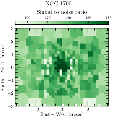
To increase the S/N of the data, we use the Voronoi binning procedure of Cappellari & Copin 2003. The one-dimensional spectra are irregularly spaced in galactocentric coordinates, due to dithers and pointing offsets between individual frames, and the hexagonal shape of the IFU lenslets. Since Voronoi binning requires regularly spaced coordinates, we construct a square grid in (x,y) with a grid spacing of , equal to the width of a hexagonal lenslet. We then tag each spectrum to the nearest grid point. We do not consider overlap with multiple grid points – each spectrum is given 100% weight at a single grid position.
The Voronoi binning procedure does not co-add the spectra, but merely defines the bins based on the estimated signal and noise of each point on the regular grid. For each grid point, we estimate the fluxes and the pixel-to-pixel variance of all contributing spectra by using the residuals between the observed spectra and boxcar-smoothed spectra over a 10 pixel window. The signal assigned to each grid point is then the sum of the fluxes of all contributing spectra, while the noise is the quadrature sum of the contributing spectra noise. We use a custom implementation of the binning step that imposes spatial symmetry over four galaxy quadrants. The bin boundaries are then used to create symmetric bins in the remaining three quadrants. The data (i.e. the 1-D spectra) is never folded during this step. We use a Voronoi binning target S/N of 125, which results in high quality spectra that do not sacrifice the spatial resolution of the innermost bins. The resulting S/N per bin values generally scatter around the target, with a typical RMS scatter of , as can be seen in Fig. 1.
In most cases, a Voronoi bin is composed of multiple grid segments, each affiliated with multiple one-dimensional spectra, usually from different exposures. The final step is to co-add all of the one-dimensional spectra in each Voronoi bin and to create a corresponding Gaussian kernel for the instrumental resolution of the co-added spectrum. This is done with a clipped 3- mean and rescaling for regions overlapping the chip gaps at one of the two wavelength settings.
IV Measuring stellar kinematics
The stellar LOSVD is extracted using the penalized pixel-fitting (pPXF) method of Cappellari & Emsellem 2004, which convolves a set of template stellar spectra with the LOSVD function . The latter is modeled as a Gauss-Hermite series of order up to (Gerhard 1993; van der Marel & Franx 1993):
| (1) |
where , is the mean velocity, is the velocity dispersion, and is the Hermite polynomial as defined in Appendix A of van der Marel & Franx 1993.
For each binned spectrum we fit all six Gauss-Hermite moments, although for brevity we only show the first four moments in our kinematic plots. We run pPXF with an initial guess of 0 for and through , and 300 km s-1 for . As our model continuum fit, we use an additive polynomial of degree zero (i.e. an additive constant) and a multiplicative polynomial of degree three. In cases where the LOSVD is undersampled or the S/N is low, it is important to use the pPXF penalty term to suppress the large uncertainties of the higher order moments (Cappellari & Emsellem 2004). Since the galaxies in our sample have large velocity dispersions and the data have high S/N, it is not critical that we penalize deviations from a Gaussian solution – hence we set the pPXF keyword BIAS to zero.
Prior to fitting, we center the spectra on the triplet of calcium absorption features by cropping close to the wavelength range 8420 – 8770 Å. We also mask any prominent residual sky lines. That is, we mask small wavelength regions centered on the locations where the sky lines occur. Overall, this corresponds to excluding or less of the fit region. We present example pPXF fits at the nucleus, in an intermediate and in an outer spatial bin for NGC 1700 in Fig. 2.
Barth et al. 2002 tested the robustness of using the Ca triplet spectral region for velocity dispersion measurements. Similar to Dressler 1984, they found little sensitivity in the measurements to the choice of template stars. We performed our own template mismatch tests using two different sets of template stars chosen from the CaT Library of 706 stars in Cenarro et al. 2001. The first template set contains the identical 15 K and G stars as in Table 2 of Barth et al. 2002. The second template set contains all G and K stars in the CaT Library. For the latter, we ran pPXF for all the bins in one of our 20 galaxies and examined the 40 stars that were assigned the highest weights. Only one of the 40 stars is in common with the 15 stars in Barth et al. 2002. Despite the difference in the two template choices, we find that the rms difference in the kinematic moments measured from the two sets of templates is km s-1 for and , and for and , well within the measurement errors of km s-1 and , respectively. We therefore confirm that our kinematic measurements are robust to template choices. The results reported in this paper use the 15 template stars in Barth et al. 2002.
We note that we performed similar tests in Veale et al. 2017b for the Mitchell IFU data in the wavelength range Å. The results there also indicated that our kinematic measurements are relatively insensitive to the choice of input template library.
The stellar spectra in the CaT Library cover the wavelength range 8348 – 9020 Å with a spectral resolution of 1.5 Å FWHM. To match the spectral resolution of our binned spectra, we convolve the templates with a Gaussian distribution with appropriate dispersion. We determine the instrumental resolution of our data by using the known sky lines prior to sky subtraction, as described in Section III, or arc lines from the CuAr calibration lamp. We first fit a Gaussian to each individual sky or arc line. Then we fit a low-order polynomial to the full width at half-maximum (FWHM) of the lines versus wavelength and determine the corresponding FWHM for our fit region centered at Å. We determine this best-fitting FWHM for each individual lenslet of each exposure. Typical values for the FWHM are Å, with variations of Å with lenslet position. This corresponds to an instrumental resolution of km s-1 at 8600 Å with a sampling of 0.67 Å per pixel. Finally, we generate a Gaussian kernel for each binned spectrum by averaging the kernels of each individual lenslet assigned to that bin. While it is possible for the line spread function to deviate mildly from a Gaussian shape (e.g., slightly flat-topped for the KCWI spectrograph; Morrissey et al. 2018; van Dokkum et al. 2019), in practice the uncertainty in the LSF introduces non-negligible bias in the recovery of the kinematic moments only when the measured velocity velocity dispersion is smaller than the instrumental dispersion (Cappellari 2017). Typical velocity dispersions for MASSIVE galaxies are km s-1, much higher than the spectral resolution of GMOS ( km s-1). Uncertainties in the LSF are therefore subdominant to other sources of systematic error.
The error bars on the kinematic moments are obtained through a bootstrap approach. This choice is motivated by the fact that each Voronoi bin contains tens (inner bins) to hundreds (outer bins) of individual lenslet spectra from different science exposures that have different noise properties. A bootstrap trial consists of taking the individual lenslet spectra that belong to a Voronoi bin and drawing a sample with replacement, then using this sample to generate a new co-added spectrum, which we run through pPXF to determine the best-fitting Gauss-Hermite moments. We repeat this process 100 times. Finally, the error for each kinematic moment is computed as the standard deviation of the pPXF results for the 100 bootstrap trials. Using this bootstrap approach, we find errors that are larger than the errors from a simpler Monte Carlo approach.
The Monte Carlo approach assumes the noise of the co-added galaxy spectrum to be representative of the noise for all the individual lenslets spectra that make up the co-added spectrum. Since the individual lenslets that make up a bin often come from exposures that were taken several days (or months) apart, it is very likely that there exist significant differences in the noise properties from one lenslet spectrum to the next (caused by variations in nighttime conditions, instrument performance, or spatially within the galaxy). This variation is captured only to a lesser extent by the noise estimates that are used in the Monte Carlo approach, since these are generated from the final spectrum after co-adding all the input lenslet spectra. We believe that the errors from the bootstrap approach are instead more realistic since this approach doesn’t make any assumptions about the noise properties of the data and incorporates any systematic differences between spectra extracted from different science frames and lenslets prior to co-adding.
V Velocity features
Fig. 3 (left panel) shows the radial velocity profiles measured from our GMOS IFS data along the photometric major axis of the central region of each of the 20 galaxies. Sixteen of the 20 galaxies have low rotation velocities with km s-1. Three galaxies exhibit fast central rotation, with reaching values of km s-1: NGC 1129 (light blue), NGC 1453 (orange), and NGC 2693 (magenta). The rotation speeds at to 1.5 kpc ( to ) of these three galaxies in Fig. 3 are maintained at a similar level out to one effective radius and beyond in our wide-field Mitchell IFS data, which measured a maximum of 70 km s-1, 95 km s-1, and 150 km s-1 for NGC 1129, NGC 1453, and NGC 2693, respectively (Table 1, Ene et al. 2018).
To quantify the importance of rotation relative to dispersion in the central region probed by the GMOS IFS, we compute the spin parameter measured within a circular aperture of radius 1 kpc, , where , and the brackets refer to luminosity-weighted averages. Individual values of are listed in Table 1 (column 8) and plotted in the right panel of Fig. 3. When compared to the larger-scale spin measured within one effective radius, (column 6 of Table 1), Fig. 3 (right panel) shows that the galaxies with higher featured in the left panel also have larger as well as larger . The majority of our sample galaxies, however, has both low central and low global spins and clusters in a distinct part of the - parameter space in Fig. 3.

The fourth galaxy highlighted in the left panel of Fig. 3, NGC 1700 (dark blue), shows a prominent KDC in our GMOS data. This component rotates in exactly the opposite direction of the main body rotation (see Fig. 4). The existence of this counter rotating core (CRC) was first pointed out by Franx et al. 1989 and later examined through detailed stellar kinematics up to four effective radii of Statler et al. 1996. Both studies used long-slit spectroscopic observations and neither achieved the high angular resolutions and high presented here.
Previous works have also uncovered kinematically distinct features at the center of ETGs. Ricci et al. 2016 studied the stellar kinematics of the circumnuclear regions of 10 massive, nearby ETGs and found a KDC with an extent of pc, while McDermid et al. 2006 found that some fast rotating SAURON ETGs have central small scale counter-rotating KDCs and that these KDCs have stellar populations that are younger than those of the main galaxy body. This is also the case for the NGC 1700 KDC, which Kleineberg et al. 2011 found to have a distinct stellar population, much younger than the main body and suggest that it formed as the result of a merger between the main galaxy and a small stellar companion on a retrograde orbit. On larger scales (), two KDCs in MASSIVE galaxies NGC 507 and NGC 5322 were detected in our wide-field Mitchell IFS data (Ene et al. 2018). The rotation axis of the inner component of NGC 507 was misaligned by from the rotation axis of the outer component, while for NGC 5322 the two components are misaligned by almost . We noted in Ene et al. 2018 that more MASSIVE galaxies may contain KDCs on smaller scales not resolvable by the diameter fibers of the Mitchell IFS. NGC 1700 is one such example.
Kinematic features such as central KDCs and any misalignment between the kinematic and the photometric axes provide useful clues about the merger history of massive ellipticals. Visual inspections of the 20 GMOS velocity maps in Appendix A suggest that the kinematic axis of the central region – when rotation is detected – is not necessarily aligned with the photometric axis (which is typically the long axis of the GMOS FOV). The relative angle ranges from well aligned (e.g., the 3 galaxies with high core rotations) to almost maximally misaligned (e.g., NGC 1700). In addition, the GMOS data now enable us to quantify how the kinematic features in the central regions of massive galaxies are connected to and aligned with the large-scale kinematic features measured from our Mitchell data in Ene et al. 2018. A detailed analysis of these properties will be presented in a separate work.
VI Velocity dispersion
VI.1 Central velocity dispersion
The high spatial sampling of the GMOS IFS enables us to measure the stellar velocity dispersion within apertures of different sizes. We measure the central stellar velocity dispersion by taking a luminosity-weighted average of within a circular aperture of radius 1 kpc. The resulting values are listed in column 9 of Table 1. We find that 6 of the 20 galaxies have high central velocity dispersion km s-1, 4 have km s-1, and the rest is in between. NGC 890 has the lowest value with km s-1.
As another measure of central , we take a luminosity-weighted average of the GMOS within an aperture of diameter, which is the size of one Mitchell IFS fiber. This GMOS can then be compared directly to the Mitchell measured from the central Mitchell fiber. Fig. 5 shows an excellent overall agreement, with a median fractional difference of .
The observed rms scatter in the difference of the two velocity dispersion measurements is km s-1, while the estimated scatter computed from the individual measurement errors is km s-1. Since the GMOS is an average of the velocity dispersion over many spatial bins, each of which is measured from a high S/N spectrum, the statistical errors on the GMOS in Fig. 5 are very small ( km s-1) and are likely subdominant to various systematic errors. Using the measurement errors on individual GMOS bins ( km s-1) instead of the luminosity-averaged statistical erros, we find that the scatter in the difference of the velocity dispersions is in good agreement with the scatter estimated from the errors. Keeping this in mind and considering that the GMOS and Mitchell are measured using data from different instruments and telescopes over different spectral regions using different template libraries, the agreement shown in Fig. 5 is nonetheless reassuring. A similar comparison for the higher-order moments and finds that the observed rsm scatter is while the scatter estimated from the measurement errors is . Once again, accounting for the fact that the luminosity-averaged statistical errors are underestimating the observed errors (), we recover a much better agreement between the observed and estimated scatter.
We note that measuring the GMOS as a luminosity-weighted average over the dispersions from individual bins within some spatial region is not identical to measuring from a single co-added spectrum within the same spatial region (e.g., a Mitchell fiber sized aperture). To quantify this difference, we use the GMOS data to generate a co-added spectrum (where we sum all the individual lenslet spectra that fall within a diameter aperture) and derive the pPXF best-fitting kinematic moments for the co-added spectrum. Although the values computed through these two methods (luminosity-weighted average and from a co-added spectrum) are not identical, we found the differences to be small, on the order of . A few outliers correspond to galaxies with large velocity gradients in the region probed by GMOS, which the diameter Mitchell fibers do not resolve. The unresolved high velocity leads to an increase in the recovered value of Mitchell velocity dispersion. If we instead compute , we find better agreement with the Mitchell value. Veale et al. 2017b also found agreement between computed from these two methods.
VI.2 Comparison with literature
To compare the GMOS measurements with literature values of compiled in the HyperLeda catalog (Paturel et al. 2003), we compute the GMOS as a luminosity-weighted average within the aperture used by HyperLeda (0.595 kpc radius). The left panel of Fig. 6 shows good agreement between GMOS and HyperLeda values, with a median fractional difference of . The HyperLeda values are compiled from heterogeneous measurements in the literature and usually have large error bars.
Deviations of more than occur for three galaxies: NGC 315 ( km s-1 versus km s-1 in HyperLeda), NGC 1129 ( km s-1 versus km s-1 in HyperLeda), and NGC 2693 ( km s-1 versus km s-1 in HyperLeda). We note that the HyperLeda catalogue contains a large range of values for NGC 315 (260 km s-1 to 360 km s-1) and NGC 2693 (270 km s-1 to 400 km s-1).
For 18 galaxies in our sample, we can also compare the GMOS with those reported in the HET catalogue (van den Bosch et al. 2015). The HET catalogue provides stellar kinematic parameters for 1022 galaxies measured from long-slit spectra in the wavelength range 4200 – 7400 Å taken with the Marcario Low Resolution Spectrograph (Hill et al. 1998) on the Hobby-Eberly Telescope (HET) at McDonald Observatory. The HET values are measured using a aperture and the typical S/N inside the aperture is greater than 100. The right panel of Fig. 6 compares the HET with our GMOS measured within an equivalent circular aperture with radius . The median fractional difference is . We also note that for the 3 outliers with HyperLeda mentioned in the previous paragraph, our values agree better with HET: km s-1 for NGC 315, km s-1 for NGC 1129, and km s-1 for NGC 2693.
VI.3 Aperture correction
Aperture correction relations are used frequently to transform velocity dispersions measured with fiber-fed spectrographs such as SDSS to values measured within a uniform aperture of a standard physical size. These correction relations are important for systematic studies of galaxies at different distances and particularly so in the case of high redshift studies where the typical IFS fiber size covers a significant fraction of the small apparent size of the galaxies. A typical application consists of correcting the velocity dispersion of galaxies to apertures with sizes related to the effective radius, e.g., , , or . Our GMOS and Mitchell IFS data together span a wide radial coverage (from to beyond ) of each galaxy and can be used to derive an aperture correction relation between velocity dispersions measured within two commonly used radii, and .
For most of our galaxies, the coverage of the GMOS FOV corresponds to a radial extent of kpc from the center of each galaxy, allowing us to measure the value of within . Here we use measured from deep -band photometric data taken with WIRCam on the Canada-France-Hawaii Telescope as part of the MASSIVE Survey (Quenneville et al. in prep). To determine , the photometry package ARCHANGEL (Schombert 2007) is used to fit elliptical isophotes to the stacked image of each galaxy. A curve of growth is then constructed from the aperture luminosity for each isophote as a function of radius. The total luminosity and half-light radius are then measured from the curve of growth. The values of for our sample of 20 galaxies are given in column 5 of Table 1. They range from to , with the average being ( kpc).
In Fig. 7 we present the aperture correction relation between the velocity dispersion at (measured from GMOS data) and the velocity dispersion at (measured from Mitchell data). We find the mean correction to be only 4.4% but the scatter is large:
| (2) |
The fact that the average of the ratio of at the two radii is close to unity by no means implies that the radial profiles of are flat between and . The diverse radial profiles of are evident in Figs. 16-25 of Appendix A and are reflected in the the large scatter in Eqn. 2.
Four galaxies in our sample were identified in Veale et al. 2018 as having rising outer velocity dispersion profiles (green points in Fig. 7). These galaxies have higher at than at . When these four galaxies are excluded, the ratio increases to .
The fact that the ratio of the two measurements is so close to unity could also be caused by luminosity-weighting, which biases to higher values by assigning more weight to the inner bins. On average, the luminosity-weighted is km s-1 higher than the corresponding arithmetic average. Using the arithmetic average value for for all 20 galaxies leads to a ratio of .
The aperture correction reported here is in agreement with our earlier measurement of using the Mitchell data for the 41 brightest MASSIVE galaxies (Veale et al. 2017b). For 40 ETGs with lower mass than our sample, the SAURON IFU data gave a higher mean aperture correction but a comparably large scatter: (Cappellari et al. 2006). Other aperture correction studies for nearby ETGs found a ratio of 1.087 using a compilation of kinematic and photometric data from literature for 51 E and S0 galaxies (Jorgensen et al. 1995), and a ratio of 1.133 from long-slit spectroscopic data for 35 ETGs in the Coma cluster (Mehlert et al. 2003), but neither work reported error bars.
VI.4 Velocity dispersion radial profiles
Fig. 8 shows the velocity dispersion as a function of radius from to from our GMOS (purple circles) and Mitchell (green squares) IFS data. For more details, see the individual kinematic maps and radial profiles (unfolded along the IFU PA) of the four velocity moments , and in Appendix A. In the inner few arcsecs, the profiles for most galaxies in our sample decrease from peak values close to the galaxy centers to smaller values further out.
In the transition region at – , the GMOS values are well matched to the Mitchell values, with the exception of a few cases such as NGC 1129 and NGC 2693. These galaxies represent the outliers mentioned at the end of Section VI.1 with high GMOS velocity gradients that cannot be resolved by the diameter Mitchell fiber(s) and for which the velocity dispersion of the inner few Mitchell fibers should be compared to measured from the GMOS data. It should also be noted that the exact location of the innermost Mitchell data point in each radial plot in Fig. 8 is uncertain to within a few arcsecs due to the large diameter of the Mitchell fiber.
For most galaxies continues to decrease in the region probed by Mitchell data. We find that at large radii is typically smaller than near the center by – 150 km s-1. Four galaxies – NGC 545, NGC 741, NGC 1129 and NGC 4874 – have rising profiles towards larger radii, with NGC 1129 and NGC 4874 showing the most prominent rise. The one outlier is NGC 890, whose has a peak value at and decreases gently both towards smaller and larger radii.
We quantify in the central region probed by GMOS using a single power law: . The best-fit logarithmic slope for each galaxy is given in column 10 of Table 1, and each best-fitting profile is shown as a blue straight line over the radial range used in the fit in Fig. 8. We use only data points beyond for the fit to mitigate the effects of seeing that can flatten the shape of in the innermost part. The profiles from to are reasonably approximated by a single power law, with the exception of NGC 315 and NGC 1700, which show a break at . For these two galaxies we restrict the fit to . Our aim here is to find a simple form to approximate the shape of the GMOS outside of , and for this purpose, a single power-law provides a reasonable fit to the data. All galaxies have per degree of freedom (DOF) or less, with the exception of NGC 1129 which has per DOF . We do not think it is worthwhile to attempt to find a closer fit to the diverse shapes of using a more complicated functional form with PSF convolution. Instead, we will perform full dynamical modeling using the complete 2D measurements of as well as other kinematic moments and will report the results in later papers.
We find that 19 out of the 20 galaxies have negative , i.e., increases from inward. To compare the central behavior of with that at larger radii, we compare with the logarithmic slope of at the effective radius. For the latter, we measure using the wide-field Mitchell data to fit a broken power law to (Veale et al. 2018), and then use the asymptotic logarithmic slopes and to compute the local logarithmic slope at . The two slopes and are plotted in Fig. 9. In contrast to the negative , is spread out from to . Furthermore, more than half of the galaxies have , i.e., changes logarithmic slopes in the inner and rises more steeply towards the galaxy’s center.
Loubser et al. 2018 measured the slopes of the velocity dispersion profiles using long-slit spectroscopic observations of a combined sample of brightest cluster galaxies (BCGs) and brightest group galaxies (BGGs). The radial coverage of their long-slit data extends up to kpc for BGGs and kpc for BCGs. For the five GMOS galaxies in common with their BGG sub-sample, Loubser et al. 2018 found negative slopes. The values are shown in Table 2, along with our own measurements of and . The Loubser et al. 2018 values of the velocity dispersion slope are in good agreement with our own for all five galaxies and in moderate agreement with , except for NGC 410.
| Galaxy | |||
|---|---|---|---|
| NGC0315 | |||
| NGC0410 | |||
| NGC0777 | |||
| NGC1060 | |||
| NGC1453 |
Note. — (1) Galaxy name. (2) Velocity dispersion logarithmic slope at 1 kpc, measured from the GMOS IFS data. (3) Velocity dispersion logarithmic slope at the effective radius, measured from the Mitchell IFS data. (4) Velocity dispersion logarithmic slope measured by Loubser et al. 2018.
An increase in the line-of-sight towards small radii can be accounted for by the presence of either a central mass concentration (e.g., a black hole) or radial anisotropy at small radii (Binney & Mamon 1982; Gerhard et al. 1998). This mass-velocity anisotropy degeneracy can be broken somewhat by using information about the LOSVD kurtosis , which we will discuss in Section VII. Our dynamical modeling of the full set of kinematic moments () will determine which combination of velocity anisotropy and mass profiles would best fit the data presented in this paper. Prior such modeling of a handful of massive elliptical galaxies have found tangential velocity anisotropy and massive black holes in the central regions and radial velocity anisotropy at larger radii (Gebhardt et al. 2000; Gebhardt et al. 2003; Shen & Gebhardt 2010; Gebhardt et al. 2011; McConnell et al. 2012; Thomas et al. 2014; Thomas et al. 2016).
VII Higher-Order Velocity Moments
VII.1 Skewness
In Fig. 10 of Veale et al. 2017b, we examined the behavior of the two odd velocity moments and on scales of kpc up to kpc measured from the Mitchell IFS data for a sample of MASSIVE galaxies. For the fast rotators (), we found a clear anti-correlation between the spatially-resolved and within each galaxy. The slope of the anti-correlation, , ranged between and . The slow rotators (), on the other hand, showed positive, negative or no correlations between the two odd moments. This result is consistent with the interpretation that anti-correlations between and within a galaxy are associated with its internal disc kinematics (Bender et al. 1994), and only fast-rotating ETGs exhibit such features.
The high-resolution GMOS IFS data now enable us to extend this analysis to the core regions of 20 ETGs in the MASSIVE survey. As shown in Fig. 10 (top panel), we find a clear anti-correlation between and for the four galaxies (NGC 1129, NGC 1453, NGC 1700, NGC 2693) with noticeable core rotations in Fig. 3. Since the rotations continue from kpc to and beyond (see Section V), these four galaxies have relatively high spin parameters (measured at both 1 kpc and ): and and , respectively.
The slope of the spatially-resolved and measured within each galaxy is plotted against the galaxy spin parameter for all 20 MASSIVE galaxies in the bottom panel of Fig. 10. For the faster rotators with above 0.1, the anti-correlation slopes are between and , similar to the range measured on larger scales in Veale et al. 2017b. The large spread in the slopes with both positive and negative values for the remaining galaxies is also similar to that seen on large scales for slow rotators in Veale et al. 2017b.
As described in Section V, NGC 1700 has a counter-rotating core that rotates in exactly the opposite direction from the main body rotation. Despite its relatively low central rotation ( km s-1; Fig. 3), the and within the core region of NGC 1700 show a steep anti-correlation with a slope of . Hints of anti-correlation for galaxies with counter-rotating cores or kinematically decoupled components have also been found in lower-mass ETGs in the ATLAS3D survey (Krajnović et al. 2011).
VII.2 Kurtosis
In Fig. 11 we compare the luminosity-weighted average measured within kpc using the GMOS data to the luminosity-weighted average measured within one effective radius using the Mitchell data. On both small and large scales, we find that the average is predominantly positive: 14/20 galaxies have and 18/20 galaxies have . We have previously found that MASSIVE galaxies show predominantly positive large scale average that is in of cases accompanied by a rising outer velocity dispersion profile (Veale et al. 2017b; Veale et al. 2018).
As mentioned in Section VI, can help break the degeneracy between the effects of mass and velocity anisotropy on the behavior of the line-of-sight velocity dispersion. For example, Veale et al. 2018 found a statistically significant positive correlation between the radial gradient in and the velocity dispersion outer logarithmic slope for a sample of 90 MASSIVE galaxies. They argue that this trend is more likely due to mass profile variations than to velocity anisotropy, since radial anisotropy at large radii would imply that a positive gradient comes along with a more negative gradient. Their arguments applied to the behavior of and (and the implications for mass and velocity anisotropy) at large radii, where the dominant contribution comes from the dark matter halo mass.
By contrast, the GMOS data studied here probe the central regions of galaxies in which stars and possibly black holes dominate the mass. In Fig. 12 we plot the radial gradient versus the velocity dispersion logarithmic slope for the core region of the galaxies in our sample. We do not find any significant correlation between the radial gradient and the velocity dispersion slope for the sample as a whole. Even after excluding the outlier NGC 890, the -value of the significance of correlation for a linear fit to the data (with slope ) is . However, we note that 14 out of 19 galaxies with negative have positive gradients (and positive values in general, as shown in Fig. 11).
For galaxies without central black holes, the information about can be used to infer the velocity dispersion anisotropy: at small radii close to the galaxy center, various types of models predict that tangential anisotropy produces a peaked LOSVD (), while radial anisotropy gives a flat-top LOSVD () (Bender et al. 1994 and references therein). However, using information about alone to estimate the effect of a black hole on the LOSVD and/or the anisotropy profile is not as straightforward. For example, Baes et al. 2005 studied a two-parameter family of isotropic models with a central black hole. They found that the profile is significantly affected by the presence of a central black hole for the isotropic models with shallow central density profiles (i.e. the central regions show positive peaks), but didn’t see any effects for models with steep density cusps. Additionally, there are several cases of SMBHs with measured negative where Schwarzschild orbit modeling predicts tangential anisotropy in the galaxy center (Pinkney et al. 2003; Gebhardt et al. 2003; McConnell et al. 2012). This behavior was also reproduced by merger simulations of dynamical systems with central SMBHs that have produced cases with central tangential anisotropy and negative , particularly in the systems with higher SMBH masses (Rantala et al. 2018).
Comparing to the isotropic models of Baes et al. 2005, the fact that our galaxies do not exhibit central positive peaks suggests that, if the data resolve the black hole SOI, then the galaxies are unlikely to be isotropic. The simulations of Rantala et al. 2018 further suggest that central tangential anisotropy could explain the low observed , but detailed dynamical modeling is needed to make any robust statements about the behavior of the velocity anisotropy in the center of galaxies.
VIII Jeans modeling
The stellar kinematics over the large radial coverage of the combined GMOS and Mitchell datasets provide powerful constraints on the mass components in ETGs. Here we apply the computationally simple method of Jeans Anisotropic Modeling (JAM; Cappellari 2008) to illustrate how the two datasets can be used to infer the central black hole mass, the stellar mass-to-light ratio and the dark matter halo content of the regular fast rotator NGC 1453 in our sample.
We choose NGC 1453 due to its regular photometric properties and almost purely elliptical isophotes (Fig. 13; Goullaud et al. 2018). In addition to being a regular fast-rotator, Ene et al. 2018 showed that the photometric and kinematic position angles of NGC 1453 are almost perfectly aligned, suggesting that the galaxy may be modeled as an axisymmetric system. As an interesting note, NGC 1453 also contains a large () warm ionized gas disc that is rotating almost perpendicularly to the stellar kinematic axis, suggesting that the gas accreted through external processes (Pandya et al. 2017).
The rest of our sample is either slowly rotating and/or shows kinematic and photometric twists. The orbit superposition model (Schwarzschild 1979) is likely a more suitable method for determining the dynamical masses of these galaxies. Orbit modeling results are beyond the scope of the present paper and will be reported in future work.
VIII.1 Mass Model
We assume that the mass in each galaxy consists of three parts: a central black hole, a stellar mass component and a dark matter halo. To model the stellar component we use the Hubble Space Telescope Wide Field Camera 3 (WFC3) IR photometry in the filter F110W from Goullaud et al. 2018. The surface brightness is fitted using the Multi-Gaussian Expansion (MGE) method (Emsellem et al. 1994; Cappellari 2002) with a sum of 2-dimensional Gaussian components that share a common center and position angle:
| (3) |
where and are projected coordinates measured from the galaxy center, with being along the photometric major axis. The subscript labels the individual Gaussian components, , , are the luminosity, dispersion and projected axis ratio of each Gaussian respectively. To obtain the MGE fit, the model predictions need to be convolved with the point spread function (PSF), which is taken from Goullaud et al. 2018, and is also expressed as an MGE using 5 nearly-circular Gaussian components (with axis ratios ). Our best-fit MGE to the surface brightness of NGC 1453 consists of 11 Gaussian components, which are summarized in Table 3 and plotted in Fig. 13. The small fitting residuals (bottom panel) demonstrate that the MGE model agrees very well with the data.


Given an inclination and stellar mass-to-light ratio , the 2-dimensional MGE fit can be deprojected and converted into a realistic 3-dimensional stellar mass density profile. Throughout this work we assume an edge-on orientation (inclination of ) and a spatially constant .
We parametrize the dark matter halo using a two-parameter logarithmic potential:
| (4) |
where is the characteristic radius of the halo potential and is the circular speed at (such a DM description was, e.g., favored by orbit-based models of M87 in Murphy et al. 2011). The logarithmic potential corresponds to a density profile given by (Binney & Tremaine 2008):
| (5) |
Before being passed to JAM, the dark matter density profile is fitted using a 1-dimensional MGE model.
VIII.2 Modeling velocity anisotropy
We augment the four parameters describing the mass profile with a description for the anisotropy,
| (6) |
which quantifies the flattening of the velocity ellipsoid along the minor axis.
Previous works with JAM have typically assumed a globally constant , although there have been some attempts at introducing moderate spatial variation, by having vary between the different Gaussian components of the MGE (e.g., Cappellari et al. 2015). The large radial span of our combined two data sets motivates including at least some spatial dependence. Perhaps most importantly, our model should distinguish between the core and the outskirts of the galaxy. The core-like part of the light profile of massive galaxies is commonly interpreted as being the result of black hole scouring (Faber et al. 1997), which in turn predicts a bias towards tangential orbits in the centre and more radial orbits in the outskirts (Quinlan & Hernquist 1997; Milosavljević & Merritt 2001). In order to at least partially replicate orbit-type variation, we assign separate anisotropies to the Gaussians with and the Gaussians with . The choice of is motivated by the fact that the light profile of NGC 1453 starts to fall off more steeply once (see bottom panel of Fig. 13).
VIII.3 Fitting the kinematic data
Our mass model is specified by six parameters: , , , , and . JAM places constraints on these parameters by comparing the model predictions for (including instrumental PSF convolution) to the observed for each Voronoi bin. We use the GMOS PSF (modeled as a Gaussian with dispersion ) since the PSF is most important near the center, at the locations of the GMOS data points. We compute the PSF by fitting a Gaussian function to point sources from the GMOS acquisition images, which are usually taken before a group of 3 – 4 science exposures. The final PSF estimate is a weighted average of the Gaussian FWHMs, weighed by the total exposure time of the group of science exposures that each acquisition image precedes. In the fit, we exclude the few Mitchell kinematic points with since this region is better measured by GMOS.
We find the JAM parameters by first running a broad regular-grid search, followed by a best-fit estimation using Bayesian inference. We calculate the posterior probability distribution using an implementation (Cappellari 2013) of the Adaptive Metropolis algorithm of Haario et al. 2001. The best-fitting model (with 3 errors) is , , , , and .
The of a large suite of JAM models shows a clear minimum for each of the six mass model parameters (Fig. 14). The constraints on the two dark matter halo parameters are weaker primarily because at , . As a result, there is significant degeneracy between the two halo parameters. The negative and positive of our best-fit model indicate a radially increasing profile (the profile that can be obtained from the best-fit is not a step function, but smoothly increasing from at small radii to outside of the core) 11 1 We also ran JAM with the two-component replaced by a single, constant . The resulting best-fit model (, , , , ) produces a worse fit, with .. JAM’s cannot be directly related to tangential/radial anisotropy (defined in spherical coordinates), but our data clearly favors a velocity anisotropy that is different in the inner and outer parts of the galaxy. Figure 15 shows our best-fitting predictions, demonstrating that the trends in both the GMOS () and Mitchell () data sets can be well reproduced by JAM and a model without a central black hole fails to reproduce the observed kinematics at small radii.
While JAM is plausibly a suitable method for NGC 1453 and other fast rotators, the utility of JAM is limited by its assumptions of axisymmetry, cylindrically aligned velocity ellipsoids and by the issue that its solutions could be unphysical. These assumptions are not well motivated in slowly rotating, triaxial ETGs, which constitute the majority of our galaxies. Furthermore, the MGE-based anisotropy profiles, which are globally constant or with limited spatial variation, may be too simplistic for representing a galaxy’s true anisotropy structure. Future papers in the MASSIVE survey series will present results from full-scale dynamical mass modeling using stellar orbit libraries that take advantage of the full set of kinematic moments from GMOS and Mitchell observations (Liepold et al. in preparation; Quenneville et al. in preparation).
IX Conclusions
We have presented the first results from the high spatial-resolution spectroscopic component of the MASSIVE survey. The spatially-resolved spectroscopic observations were obtained with the Gemini GMOS-N IFS for the central (about 2 kpc across) regions of 20 ETGs in the MASSIVE survey. These galaxies have () and are located at a median distance of Mpc. We measured the stellar kinematics from high- () spectra using a Gauss-Hermite parameterization of the LOSVD. We obtained two-dimensional maps of the first four kinematic moments (, , , and ) and compared them to the large-scale stellar kinematics obtained from the Mitchell IFS (Veale et al. 2017b; Veale et al. 2017a; Veale et al. 2018). The two IFS datasets together cover a length scale of , or kpc. Our main findings are as follows:
- •
The velocity maps of most galaxies in the sample show some level of rotation in the central regions (upper left panel in Figs. 16-25 of Appendix A). Three galaxies (NGC 1129, NGC 1453, and NGC 2693) exhibit fast rotations with rising up to km s-1 within 1 kpc, and a fourth galaxy (NGC 1700) has a counter-rotationg core that rotates in the opposite direction of the main body rotation (Fig. 3 and Fig. 4). These 4 galaxies also have noticeable rotation out to one effective radius, . The rest of the galaxies have central rotations (if detected) with km s-1, as well as low velocity rotation up to (). The kinematic axis of the central rotation is not necessarily aligned with the photometric axis or the large-scale kinematic axis, indicating a diverse merger history within this sample of 20 high-mass ETGs.
- •
The velocity dispersion within kpc reaches km s-1 or beyond in 6 of the 20 galaxies and is greater than 250 km s-1 for 14 galaxies. We measure the luminosity-weighted average within an aperture of radius versus and find an aperture correction relation of (Fig. 7).
- •
For all but one galaxy, the velocity dispersion profiles in the radial range of are well fit by a single power law form with negative logarithmic slope (Fig. 8). A rising towards smaller radii is indicative of the presence of a central SMBH but can also be caused by central radial anisotropy in the stellar velocities. On large scales, by contrast, the logarithmic slope of at ranges from to , reflecting varying degrees of contributions from dark matter mass as well as velocity anisotropies. We will use the observed higher-order velocity moment to break this mass-anisotropy degeneracy in future dynamical mass modeling work.
- •
For the galaxies with clear rotation in the inner kpc, the spatially-resolved skewness in this region is anti-correlated with the velocity, i.e., the spatial bins with higher values have more negative . The slope of this correlation, , ranges between and for the galaxies with relatively high spins in our sample (). The - anti-correlation within a galaxy indicates disc-like kinematics in both the core and main body of fast-rotating massive ETGs.
- •
The kurtosis is generally positive, with 14 of the 20 galaxies having a positive average within kpc, and 18 of them having positive average within (Fig. 11). Most galaxies also show a rising or flat radial profile . In the absence of a central mass, peaked LOSVDs () at small radii are often associated with tangential anisotropy, which tends to lower the central line-of-sight . Yet 19 out of the 20 galaxies in this study are observed to have that increase towards the center. The presence of central black holes is a possible explanation. We will perform full-scale stellar orbit modeling to determine the velocity structures, stellar and dark matter mass distributions, and black hole masses in these galaxies.
- •
Using the GMOS and Mitchell stellar kinematics, we applied the Jeans modeling method to measure the mass distributions in NGC 1453, the most regular fast rotator in our sample. To partially account for spatial variations in the stellar velocity anisotropy, we allow the anisotropy parameter in the inner and outer parts of the galaxy to be different. The JAM results show that our kinematics point towards a nonzero central black hole mass and a spatially varying velocity anisotropy. The best-fit mass model (with 3 errors) has a black hole mass of , a stellar mass-to-light ratio of (in WFC3 F110W band), and a circular velocity of km s-1 for the dark matter halo.
High spatial-resolution kinematics that resolve the sphere of influence of the SMBH are a key requirement for any attempt at black hole mass determination through dynamical modeling. Combining the small scale results presented here with the large-scale kinematics of previous MASSIVE papers will allow us to model the mass distributions of nearby massive ETGs and study their assembly histories. New SMBH mass measurements will help refine the various correlation relations between black holes and their host galaxy properties. In particular, the high-mass range sampled by our galaxy sample may be relevant for the exploration of the saturation at high (e.g., Lauer et al. 2007; McConnell et al. 2011; McConnell et al. 2012; McConnell & Ma 2013; Kormendy & Ho 2013).
Appendix A Kinematic moments plots


References
- Allington-Smith et al. (2002) Allington-Smith, J., Murray, G., Content, R., et al. 2002, PASP, 114, 892, doi: 10.1086/341712
- Baes et al. (2005) Baes, M., Dejonghe, H., & Buyle, P. 2005, A&A, 432, 411, doi: 10.1051/0004-6361:20041907
- Barth et al. (2002) Barth, A. J., Ho, L. C., & Sargent, W. L. W. 2002, AJ, 124, 2607, doi: 10.1086/343840
- Bender et al. (1994) Bender, R., Saglia, R. P., & Gerhard, O. E. 1994, MNRAS, 269, 785, doi: 10.1093/mnras/269.3.785
- Binney & Mamon (1982) Binney, J., & Mamon, G. A. 1982, MNRAS, 200, 361, doi: 10.1093/mnras/200.2.361
- Binney & Tremaine (2008) Binney, J., & Tremaine, S. 2008, Galactic Dynamics, 2nd edition), p. 75
- Brodie et al. (2014) Brodie, J. P., Romanowsky, A. J., Strader, J., et al. 2014, ApJ, 796, 52, doi: 10.1088/0004-637X/796/1/52
- Brough et al. (2011) Brough, S., Tran, K. V., Sharp, R. G., von der Linden, A., & Couch, W. J. 2011, 414, L80, doi: 10.1111/j.1745-3933.2011.01060.x
- Bundy et al. (2015) Bundy, K., Bershady, M. A., Law, D. R., et al. 2015, ApJ, 798, 7, doi: 10.1088/0004-637X/798/1/7
- Cappellari (2002) Cappellari, M. 2002, MNRAS, 333, 400, doi: 10.1046/j.1365-8711.2002.05412.x
- Cappellari (2008) Cappellari, M. 2008, MNRAS, 390, 71, doi: 10.1111/j.1365-2966.2008.13754.x
- Cappellari (2013) —. 2013, ApJ, 778, L2, doi: 10.1088/2041-8205/778/1/L2
- Cappellari (2017) Cappellari, M. 2017, MNRAS, 466, 798, doi: 10.1093/mnras/stw3020
- Cappellari & Copin (2003) Cappellari, M., & Copin, Y. 2003, MNRAS, 342, 345, doi: 10.1046/j.1365-8711.2003.06541.x
- Cappellari & Emsellem (2004) Cappellari, M., & Emsellem, E. 2004, PASP, 116, 138, doi: 10.1086/381875
- Cappellari et al. (2006) Cappellari, M., et al. 2006, MNRAS, 366, 1126, doi: 10.1111/j.1365-2966.2005.09981.x
- Cappellari et al. (2011) —. 2011, MNRAS, 413, 813, doi: 10.1111/j.1365-2966.2010.18174.x
- Cappellari et al. (2015) Cappellari, M., Romanowsky, A. J., Brodie, J. P., et al. 2015, ApJ, 804, L21, doi: 10.1088/2041-8205/804/1/L21
- Cenarro et al. (2001) Cenarro, A. J., Cardiel, N., Gorgas, J., et al. 2001, MNRAS, 326, 959, doi: 10.1046/j.1365-8711.2001.04688.x
- Croom et al. (2012) Croom, S. M., Lawrence, J. S., Bland-Hawthorn, J., et al. 2012, MNRAS, 421, 872, doi: 10.1111/j.1365-2966.2011.20365.x
- Dressler (1984) Dressler, A. 1984, ApJ, 286, 97
- Emsellem et al. (1994) Emsellem, E., Monnet, G., & Bacon, R. 1994, A&A, 285, 723
- Emsellem et al. (2004) Emsellem, E., Cappellari, M., Peletier, R. F., et al. 2004, MNRAS, 352, 721, doi: 10.1111/j.1365-2966.2004.07948.x
- Ene et al. (2018) Ene, I., Ma, C.-P., Veale, M., et al. 2018, MNRAS, 479, 2810, doi: 10.1093/mnras/sty1649
- Faber et al. (1997) Faber, S. M., Tremaine, S., Ajhar, E. A., et al. 1997, Astronomical Journal, 114, 1771, doi: 10.1086/118606
- Franx et al. (1989) Franx, M., Illingworth, G., & Heckman, T. 1989, ApJ, 344, 613, doi: 10.1086/167830
- Gebhardt et al. (2011) Gebhardt, K., Adams, J., Richstone, D., et al. 2011, ApJ, 729, 119, doi: 10.1088/0004-637X/729/2/119
- Gebhardt et al. (2000) Gebhardt, K., Richstone, D., Kormendy, J., et al. 2000, AJ, 119, 1157, doi: 10.1086/301240
- Gebhardt et al. (2003) Gebhardt, K., Richstone, D., Tremaine, S., et al. 2003, ApJ, 583, 92, doi: 10.1086/345081
- Gerhard et al. (1998) Gerhard, O., Jeske, G., Saglia, R. P., & Bender, R. 1998, in Astronomical Society of the Pacific Conference Series, Vol. 136, Galactic Halos, ed. D. Zaritsky, 248. http://adsabs.harvard.edu/abs/1998ASPC..136..248G
- Gerhard (1993) Gerhard, O. E. 1993, Monthly Notices of the Royal Astronomical Society, 265, 213, doi: 10.1093/mnras/265.1.213
- Goullaud et al. (2018) Goullaud, C. F., Jensen, J. B., Blakeslee, J. P., et al. 2018, ApJ, 856, 11, doi: 10.3847/1538-4357/aab1f3
- Greene et al. (2015) Greene, J. E., Janish, R., Ma, C. P., et al. 2015, ApJ, 807, 11, doi: 10.1088/0004-637X/807/1/11
- Greene et al. (2019) Greene, J. E., Veale, M., Ma, C.-P., et al. 2019, arXiv e-prints, arXiv:1901.01271. https://arxiv.org/abs/1901.01271
- Haario et al. (2001) Haario, H., Saksman, E., & Tamminen, J. 2001, Bernoulli, 7, 223
- Hill et al. (1998) Hill, G. J., Nicklas, H. E., MacQueen, P. J., et al. 1998, in Proc. SPIE, Vol. 3355, Optical Astronomical Instrumentation, ed. S. D’Odorico, 375–386
- Hook et al. (2004) Hook, I. M., Jørgensen, I., Allington-Smith, J. R., et al. 2004, PASP, 116, 425, doi: 10.1086/383624
- Jimmy et al. (2013) Jimmy, Tran, K.-V., Brough, S., et al. 2013, ArXiv e-prints. https://arxiv.org/abs/1310.7587
- Jorgensen et al. (1995) Jorgensen, I., Franx, M., & Kjaergaard, P. 1995, MNRAS, 276, 1341, doi: 10.1093/mnras/276.4.1341
- Kleineberg et al. (2011) Kleineberg, K., Sánchez-Blázquez, P., & Vazdekis, A. 2011, ApJ, 732, L33, doi: 10.1088/2041-8205/732/2/L33
- Kormendy & Ho (2013) Kormendy, J., & Ho, L. C. 2013, ARA&A, 51, 511, doi: 10.1146/annurev-astro-082708-101811
- Krajnović et al. (2011) Krajnović, D., Emsellem, E., Cappellari, M., et al. 2011, MNRAS, 414, 2923, doi: 10.1111/j.1365-2966.2011.18560.x
- Lauer et al. (2007) Lauer, T. R., et al. 2007, ApJ, 662, 808, doi: 10.1086/518223
- Lena (2014) Lena, D. 2014, ArXiv e-prints. https://arxiv.org/abs/1409.8264
- Loubser et al. (2018) Loubser, S. I., Hoekstra, H., Babul, A., & O’Sullivan, E. 2018, MNRAS, 477, 335, doi: 10.1093/mnras/sty498
- Ma et al. (2014) Ma, C.-P., Greene, J. E., McConnell, N., et al. 2014, ApJ, 795, 158, doi: 10.1088/0004-637X/795/2/158
- McConnell & Ma (2013) McConnell, N. J., & Ma, C.-P. 2013, ApJ, 764, 184, doi: 10.1088/0004-637X/764/2/184
- McConnell et al. (2011) McConnell, N. J., Ma, C.-P., Gebhardt, K., et al. 2011, Nature, 480, 215, doi: 10.1038/nature10636
- McConnell et al. (2012) McConnell, N. J., Ma, C. P., Murphy, J. D., et al. 2012, ApJ, 756, doi: 10.1088/0004-637X/756/2/179
- McDermid et al. (2006) McDermid, R. M., Emsellem, E., Shapiro, K. L., et al. 2006, MNRAS, 373, 906, doi: 10.1111/j.1365-2966.2006.11065.x
- Mehlert et al. (2003) Mehlert, D., Thomas, D., Saglia, R. P., Bender, R., & Wegner, G. 2003, A&A, 407, 423, doi: 10.1051/0004-6361:20030886
- Milosavljević & Merritt (2001) Milosavljević, M., & Merritt, D. 2001, ApJ, 563, 34, doi: 10.1086/323830
- Morrissey et al. (2018) Morrissey, P., Matuszewski, M., Martin, D. C., et al. 2018, ApJ, 864, 93, doi: 10.3847/1538-4357/aad597
- Murphy et al. (2011) Murphy, J. D., Gebhardt, K., & Adams, J. J. 2011, ApJ, 729, 129, doi: 10.1088/0004-637X/729/2/129
- Pandya et al. (2017) Pandya, V., Greene, J. E., Ma, C.-P., et al. 2017, The Astrophysical Journal, 837, 1, doi: 10.3847/1538-4357/aa5ebc
- Paturel et al. (2003) Paturel, G., Petit, C., Prugniel, P., et al. 2003, A&A, 412, 45, doi: 10.1051/0004-6361:20031411
- Pinkney et al. (2003) Pinkney, J., Gebhardt, K., Bender, R., et al. 2003, ApJ, 596, 903, doi: 10.1086/378118
- Quinlan & Hernquist (1997) Quinlan, G. D., & Hernquist, L. 1997, New Astronomy, 2, 533 , doi: https://doi.org/10.1016/S1384-1076(97)00039-0
- Rantala et al. (2018) Rantala, A., Johansson, P. H., Naab, T., Thomas, J., & Frigo, M. 2018, ApJ, 864, 113, doi: 10.3847/1538-4357/aada47
- Ricci et al. (2016) Ricci, T. V., Steiner, J. E., & Menezes, R. B. 2016, MNRAS, 463, 3860, doi: 10.1093/mnras/stw2318
- Roth et al. (2012) Roth, K., Schiavon, R., Chiboucas, K., & Gimeno, G. 2012, in American Astronomical Society Meeting Abstracts, Vol. 219, American Astronomical Society Meeting Abstracts #219, 422.18
- Sánchez et al. (2012) Sánchez, S. F., Kennicutt, R. C., Gil de Paz, A., et al. 2012, A&A, 538, A8, doi: 10.1051/0004-6361/201117353
- Scharwächter et al. (2018) Scharwächter, J., Chiboucas, K., Gimeno, G., et al. 2018, in Society of Photo-Optical Instrumentation Engineers (SPIE) Conference Series, Vol. 10702, 107022T
- Schombert (2007) Schombert, J. 2007, arXiv e-prints, astro. https://arxiv.org/abs/astro-ph/0703646
- Schwarzschild (1979) Schwarzschild, M. 1979, ApJ, 232, 236, doi: 10.1086/157282
- Shen & Gebhardt (2010) Shen, J., & Gebhardt, K. 2010, ApJ, 711, 484, doi: 10.1088/0004-637X/711/1/484
- Skrutskie et al. (2006) Skrutskie, M. F., Cutri, R. M., Stiening, R., et al. 2006, AJ, 131, 1163, doi: 10.1086/498708
- Statler et al. (1996) Statler, T. S., Smecker-Hane, T., & Cecil, G. N. 1996, AJ, 111, 1512, doi: 10.1086/117893
- Thomas et al. (2016) Thomas, J., Ma, C.-P., McConnell, N. J., et al. 2016, Nature, 532, 340, doi: 10.1038/nature17197
- Thomas et al. (2014) Thomas, J., Saglia, R. P., Bender, R., Erwin, P., & Fabricius, M. 2014, ApJ, 782, 39, doi: 10.1088/0004-637X/782/1/39
- van den Bosch et al. (2015) van den Bosch, R. C. E., Gebhardt, K., Gültekin, K., Yıldırım, A., & Walsh, J. L. 2015, ApJS, 218, 10, doi: 10.1088/0067-0049/218/1/10
- van der Marel & Franx (1993) van der Marel, R. P., & Franx, M. 1993, The Astrophysical Journal, 407, 525, doi: 10.1086/172534
- van Dokkum et al. (2019) van Dokkum, P., Wasserman, A., Danieli, S., et al. 2019, arXiv e-prints, arXiv:1904.04838. https://arxiv.org/abs/1904.04838
- Veale et al. (2017a) Veale, M., Ma, C.-P., Greene, J. E., et al. 2017a, MNRAS, 471, 1428, doi: 10.1093/mnras/stx1639
- Veale et al. (2018) —. 2018, MNRAS, 473, 5446, doi: 10.1093/mnras/stx2717
- Veale et al. (2017b) Veale, M., Ma, C.-P., Thomas, J., et al. 2017b, MNRAS, 464, 356, doi: 10.1093/mnras/stw2330