Blue, white, and red ocean planets
Abstract
Context. An exoplanet’s habitability will depend strongly on the presence of liquid water. Flux and/or polarization measurements of starlight that is reflected by exoplanets could help to identify exo-oceans.
Aims. We investigate which broadband spectral features in flux and polarization phase functions of reflected starlight uniquely identify exo-oceans.
Methods. With an adding-doubling algorithm, we compute total fluxes and polarized fluxes of starlight that is reflected by cloud-free and (partly) cloudy exoplanets, for wavelengths from 350 to 865 nm. The ocean surface has waves composed of Fresnel reflecting wave facets and whitecaps, and scattering within the water body is included.
Results. Total flux , polarized flux , and degree of polarization of ocean planets change color from blue, through white, to red at phase angles ranging from to for , and from to for , with cloud coverage fraction increasing from 0.0 (cloud-free) to 1.0 (completely cloudy) for , and to 0.98 for . The color change in only occurs for ranging from 0.03 to 0.98, with the color crossing angle ranging from to . The total flux of a cloudy, zero surface albedo planet can also change color, and for , an ocean planet’s will not change color for surface pressures 8 bars. Polarized flux of a zero surface albedo planet does not change color for any .
Conclusions. The color change of of starlight reflected by an exoplanet, from blue, through white, to red with increasing above 88∘, appears to identify a (partly) cloudy exo-ocean. The color change of polarized flux with increasing above 123∘ appears to uniquely identify an exo-ocean, independent of surface pressure or cloud fraction. At the color changing phase angle, the angular distance between a star and its planet is much larger than at the phase angle where the glint appears in reflected light. The color change in polarization thus offers better prospects for detecting an exo-ocean.
Key Words.
Radiative transfer – Polarization – Techniques: polarimetric – Planets and satellites: oceans – Planets and satellites: terrestrial planets1 Introduction
Liquid water is considered to be a prerequisite for life as we know it. The presence of liquid water on the surface of an exoplanet will depend on the planet’s surface temperature and therefore on the separation between the planet and its host star, the stellar luminosity, the surface albedo, the composition and structure of the planetary atmosphere (which also strongly influence the planet’s albedo) and the atmospheric surface pressure. While the amount of stellar flux that is incident on the planet can be measured, the surface albedo, and the atmospheric properties are more difficult to determine. Yet they are crucial factors in determining a planet’s habitability.
Some information about the composition and structure of the upper atmosphere of exoplanets can be derived using transit spectroscopy, where the spectral variation of the stellar flux that is transmitted through the atmosphere of a planet during its transit, is measured. Indeed, detections have been reported of water vapor in the atmospheres of hot Jupiter-like planets (Tinetti et al. 2007; Deming et al. 2013; Kreidberg et al. 2014, see for example) and a low-mass Neptune sized planet (Fraine et al. 2014). A large number of transiting exoplanets is already known, mostly thanks to the space observatories Corot (’Convection, Rotation and planetary Transits,’ by ESA/CNES) and, of course, especially Kepler (NASA). New and upcoming space observatories, like TESS (’Transiting Exoplanet Survey Satellite,’ NASA, launched in 2018, Ricker et al. 2015) and PLATO (’PLAnetary Transits and Oscillations of stars,’ ESA, planned for launch in 2026, Rauer et al. 2014), and ground-based telescope networks like WASP (’Wide Angle Search for Planets’) (Ricker et al. 2015) and MASCARA (’Multi-site All-Sky CAmeRA’) (Talens et al. 2017) are designed to search for transiting exoplanets around bright, nearby stars. Such transiting exoplanets will be excellent targets for follow-up transit spectroscopy measurements with, e.g. the JWST (the ’James Webb Space Telescope,’ NASA) and ARIEL (’Atmospheric Remote-sensing Infrared Exoplanet Large-survey,’ ESA, planned for launch after PLATO).
Transit spectroscopy, however, does not provide information about the lower atmospheric layers because the optical path-length through these layers is too large to allow the transmission of starlight, in particular in the presence of clouds. And, rocky exoplanets are so small compared to their star, and their atmospheres are so thin compared to the planetary radius, that obtaining a reliable signal-to-noise ratio could take several tens to hundreds of planetary transits. For rocky exoplanets in the habitable zones of solar-type stars, that would thus take several tens to hundreds of Earth-years (Kaltenegger & Traub 2009).
A secondary eclipse spectrum, derived from the change in the total flux spectrum when a planet starts to disappear behind and/or reappears from behind its star as seen from the observer, could provide information about the planetary albedo, and thus potentially about the planet’s surface albedo, the atmospheric gaseous scattering, and the presence of clouds (not their actual composition), although all blended together due to the lack of spatial resolution. Unless the atmospheric gaseous optical thickness, the cloud coverage fraction and the cloud physical properties (especially cloud optical thickness) are known, a secondary eclipse spectrum will thus not provide information about the planet’s surface albedo (thus, without the atmosphere) and the probability of liquid surface water (which is expected to have a very small albedo) will thus remain elusive in secondary eclipse measurements.
For identifying liquid surface water, measuring the light of the parent star that is reflected by an orbiting exoplanet, appears to be the most straightforward tool. The spectral and temporal variations of this reflected light as the planet orbits its parent star, holds information about the composition and structure of the planetary atmosphere and/or the surface (if present). This is particularly true for the state of polarization of the reflected light (see Wiktorowicz & Stam 2015, and references therein). The angular distribution of the degree of polarization of singly scattered light is much more sensitive to the size, composition and shape of the scattering particles in the exoplanet’s atmosphere than the total flux (unpolarized + polarized fluxes) is (Hansen & Travis 1974), and in addition, the angular distribution of the polarized signal is preserved when multiple light is added. In particular, the phase angles11 1 A planetary phase angle is the angle between the directions towards the parent star and the observer as measured from the center of the planet. where the degree of polarization of the reflected starlight attains a local maximum value or where it equals zero (the so-called ’neutral points’) can be directly translated into the scattering angles where the degree of polarization of the singly scattered light attains a local maximum value or zero22 2 Given a planetary phase angle , the single scattering angle equals 180.. And, because the degree of polarization is a relative measure (i.e. the ratio of the polarized flux to the total flux), it is insensitive to parameters such as distance, planetary radii, and the incoming flux. The degree of polarization is also relatively insensitive to the Earth’s atmosphere for ground-based observations, as the transmission of light through the Earth’s atmosphere is virtually independent of the state of polarization of the light (, , and are equally affected by scattering and/or absorption) and it is insensitive to several instrumental parameters (depending on the instrument design), such as the degradation of filters or lenses in time.
A famous application of these advantages of polarimetry is the characterisation of the particles composing the main cloud deck on Venus by Hansen & Hovenier 1974. They used disk-integrated polarization measurements at wavelengths across the 0.34 - 1.00 m region of Venus with Earth-based telescopes at a wide range of phase angles to determine that the clouds particles consist of 75% sulfuric acid solution, and have an effective radius of 1.05 m with an effective variance of 0.07. Because, as seen from Earth, Venus is an inner planet, it can be observed at phase angles ranging from almost 0∘ to almost 180∘, while outer Solar System planets can only be observed at small phase angles (except of course from a spacecraft in the vicinity of an outer planet). The phase angle range at which an exoplanet can be observed depends on the orbital inclination angle (defined such that for a face-on orbit), as seen from Earth: . In particular, transiting exoplanets, which TESS (Ricker et al. 2015) and PLATO (Rauer et al. 2014) are and will be searching for, will be observable across a broad phase angle range with direct detection techniques.
Simulations of orbital variations of the (polarized) flux and degree of polarization of starlight that is reflected by habitable exoplanets explore the potential observables of these planets, are crucial for the design and optimization of future instruments and telescopes aimed at the direct detection of planetary signals, and can be used to devise observational strategies (such as integration times and temporal coverage) and (future) data analysis algorithms. An example of a direct detection instrument that is designed to measure polarization of starlight reflected by exoplanets is the Exoplanet Imaging Camera and Spectrograph (EPICS) for the European Extremely Large Telescope (E-ELT) (Kasper et al. 2010). EPOL is the imaging polarimeter for EPICS (Keller et al. 2010). NASA’s LUVOIR (Large UV Optical Infrared Surveyor) space telescope concept (The LUVOIR Team 2018) includes POLLUX, a polarimeter for the ultraviolet wavelength region (Bouret et al. 2018). Another concept study by NASA is the Habitable Exoplanet Observatory (HabEx) (Gaudi et al. 2018), that, as far as we know, does not (yet) include a polarimeter.
In this paper, we focus on the numerical simulations of the total and polarized fluxes and the degree of polarization of starlight that is reflected by Earth-like exoplanets that are covered by a liquid ocean with surfaces that are rough due to the presence of waves. Fresnel reflection of light by an ocean on an exoplanet results in two main observable phenomena: a glint on the ocean surface, whose size increases with increasing surface roughness (i.e. increasing wind speed), and a maximum degree of polarization at the Brewster angle. Indeed, as the strength of both phenomena depends on the local reflection angles, they are strongly phase angle dependent.
The signatures of an ocean in the orbital variations of the total flux of starlight that is reflected by an exoplanet have been studied before. Robinson et al. 2010 modeled the phase curves of the total flux of the Earth as an exoplanet, and Oakley & Cash 2009, Cowan et al. 2009 and Lustig-Yaeger et al. 2018 aim to reconstruct a surface type map from modeled total flux phase curves at a single or multiple wavelength(s). Those papers, however, did not include the polarization of the reflected starlight. Stam 2008 computed the total flux and degree of polarization as functions of the wavelength and planetary phase angle for Earth-like exoplanets some of which with a Fresnel reflecting ocean, but did not include wind-driven waves on the ocean surface, thus yielding an infinitely narrow beam of reflected light representing the stellar glint (the spatial distribution of this glint was lost upon integration of the reflected starlight across the illuminated and visible part of the planetary disk). Williams & Gaidos 2008 presented the phase curves of an ocean planet with a rough surface and found strong signatures of Fresnel reflection in the phase angle dependence of the degree of polarization . They, however, neglected atmospheric contributions such as Rayleigh scattering and scattering by clouds. Zugger et al. 2010; Zugger et al. 2011a; Zugger et al. 2011b did include atmospheric Rayleigh scattering, and the reflection by clouds modeled as horizontal, Lambertian (i.e. isotropic and non-polarizing) reflecting surfaces33 3 Indeed, the ’rainbow peaks’ in the degree of polarization phase curves in the papers of Zugger et al. 2010; Zugger et al. 2011a; Zugger et al. 2011b are caused by their assumption of spherical maritime aerosols, not by their model clouds. It should be noted, however, that maritime (sea-salt) aerosols may be non-spherical (Mishchenko et al. 2000, see Chap. 18 of). (not only ignoring gas below and in the clouds, but also above the clouds), and scattering by maritime aerosols (modeled as spherical particles) in the cloud-free atmosphere above a rough ocean surface. They found that the ocean signature in is limited by the scattering by maritime aerosols and clouds.
The model planets of Zugger et al. 2010; Zugger et al. 2011a; Zugger et al. 2011b are horizontally homogeneous, that is, the atmosphere and surface are invariant with latitude and longitude. Therefore, they could, for example, not study the signatures of the glint appearing and hiding behind patchy clouds, which are clouds of varying horizontal shapes distributed across the planetary disk. Rossi & Stam 2017 showed the features that could potentially be observed in the flux and polarization phase curves of horizontally inhomogeneous ocean planets using various cloud cover types. Their ocean surface was, however, still a flat air-water interface, without waves, and thus with an infinitely narrow glint. Also, Karalidi et al. 2012a and Karalidi & Stam 2012 presented computed flux and polarization phase curves for horizontally inhomogeneous, cloudy Earth-like exoplanets, focusing on the signatures of the clouds, and representing the ocean by a flat, zero albedo (i.e. black) surface (without the glint).
In this paper, we present the computed planetary phase curves of the total and polarized fluxes and the degree of polarization of starlight that is reflected by oceanic exoplanets with rough, wavy surfaces beneath terrestrial-type atmospheres. We fully include scattering of (unpolarized and polarized) light within the water body (i.e. below the rough ocean surface) and the reflection by wind-generated foam on the ocean surface. We compute the phase curves for various wind speeds and surface pressures, at wavelengths ranging from 350 to 865 nm. We use two types of model ocean planets: cloud-free planets, and cloudy planets. The clouds are patchy and embedded within the gaseous atmosphere (there is thus gas below, within and above the clouds), just like those on Earth, and our model clouds consist of liquid water droplets.
This paper is structured as follows. In Sects. 2.1 and 2.2, we provide our definitions and describe our numerical method to compute both the total and polarized fluxes, and the degree of polarization of starlight that is reflected by our model ocean planets. In Sect. 2.3, we describe the physical and optical properties of the atmosphere and the ocean surface and water body below. In Sect. 3, we present the computed reflected total and polarized fluxes and for our model planets for various atmospheric and surface parameters, and we describe the influence of these parameters on the planet’s color change in total flux , polarized flux , and . In Sect. 4, we discuss the color change and with that the detectability of an ocean beneath clouds. In Sect. 5, finally, we summarize our results.
2 Numerical method
2.1 Definitions of fluxes and polarization
We describe light as the following column vector (Hansen & Travis 1974; Hovenier et al. 2004, see e.g.)
| (1) |
where describes the total flux, and the linearly polarized fluxes, and the circularly polarized flux. The dimension of these fluxes is Wm-2 or in Wm-3, when accounting for the dependence on the wavelength , but because of our normalization (see below), we do not use these dimensions explicitly. Linearly polarized fluxes and are defined with respect to a reference plane. For our computations of starlight that is reflected by a planet as a whole, we use the planetary scattering plane, i.e. the plane that contains the centers of the star, the planet, and the observer, as the reference plane. Fluxes and can be redefined with respect to another reference plane, such as an instrument’s optical plane, using a so-called rotation matrix (Hovenier & van der Mee 1983, see).
We assume that the starlight that is incident on the planet is unidirectional and unpolarized. The latter is based on the very small disk–integrated polarized fluxes of solar-type stars, as measured for active and inactive FGK–stars by Cotton et al. 2017 (with, respectively, 23 2.2 ppm and 2.9 1.9 ppm polarized flux) and Kemp et al. 1987 for the Sun itself, and the very small degree of stellar linear polarization (on the order of ) that is expected from symmetry-breaking disturbances such as spots and/or flares (Berdyugina et al. 2011; Kostogryz et al. 2015). The incident starlight is thus described as , with the stellar flux measured perpendicular to the direction of propagation, and the unit column vector.
Starlight that is reflected by a planet will become polarized by scattering by gases and aerosol or cloud particles in the planetary atmosphere and/or by reflection off the surface. We define the degree of polarization of the reflected starlight as
| (2) |
Unlike and , is independent of a reference plane. We ignore the circularly polarized flux of the reflected starlight. This flux is expected to be very small (for examples for rocky exoplanets, see Rossi & Stam 2018; García Muñoz 2015, and references therein), and ignoring circular polarization in the radiative transfer computations yields only very small errors in the total and linearly polarized fluxes (Stam & Hovenier 2005).
2.2 Calculating reflected starlight
We compute starlight that is reflected by different types of exoplanets, both the total flux and polarization, and for a range of wavelengths . Given a planet orbiting a star, with the flux vector that is incident on the planet, we compute the flux vector that is reflected by the planet as a whole and that arrives at an observer situated at a large distance of the planet and star, by integrating the locally reflected light across the illuminated and visible part of the planetary disk. We perform this integration using a grid of pixels that cover the planetary disk (Rossi et al. 2018, see), and by summing the fluxes reflected by each of the pixels that are both illuminated by the parent star and visible to the observer, as follows:
| (3) |
Here is the planetary phase angle, which is defined as the angle between the star and the observer measured from the center of the planet (at , the planet is thus behind the star as seen from the observer, and at , the planet is precisely in front of the star). Angle and the location on the planetary disk determine the local illumination and viewing angles across the planet: , with the local viewing zenith angle, , with the local illumination angle, and , the local azimuthal angle (see de Haan et al. 1987, for the precise definitions of these angles).
Matrix in Eq. 3, is a local reflection matrix, i.e. it describes how the area that pixel covers on the planet, reflects the incident light. This matrix depends on the composition and structure of the local atmosphere and the underlying surface (see Sect. 2.3), on the wavelength, as the optical properties of the atmosphere and surface are wavelength dependent, and on the local illumination and viewing angles (hence, on phase angle and/or the location of the pixel on the planet). Matrix is a rotation matrix (Hovenier & van der Mee 1983, see) that rotates each locally reflected flux vector, that is defined with respect to the local meridian plane through the local zenith and the local direction towards the observer, to the planetary scattering plane. Angle is the local rotation angle. Furthermore, is the area that grid pixel covers on the 3D-planet. The area a pixel covers on the 3D-planet depends on the local viewing angle . Indeed, equals the pixel size, which we choose the same for all pixels.
With Eq. 3, we can compute the flux vectors reflected by locally horizontally homogeneous planets, i.e. where the surface and atmosphere are the same for each pixel across the planetary disk, and by horizontally inhomogeneous planets, i.e. where the surface and atmosphere can be different for different pixels. The error that results from using the summation of Eq. 3 for the integration across the planetary disk depends on the size of the pixels, on the horizontal variations of the surface and atmosphere, and on the phase angle (Rossi et al. 2018, see). For our computations, we use a minimum of 40 pixels across the planetary equator for every , which provides a good relation between the integration error and the computing time.
To compute , we first assign an atmosphere and surface model to each pixel on the planetary disk. Then, given the phase angle , and thus the local illumination and viewing angles, the local matrices are computed and rotated using the local rotation angles . Then, the summation in Eq. 3 is evaluated. The computation of the matrices is performed with an efficient adding–doubling algorithm (de Haan et al. 1987; Stam 2008), extended with reflection by and transmission through a rough ocean surface and scattering in the ocean body (see Sect. 2.3), fully including polarization for all orders of scattering. Our adding–doubling algorithm is a multi-stream radiative transfer code. To accurately capture the angular variations in the reflected light signals, we use 130 streams for our simulations and a Fourier-series representation for the azimuthal direction (de Haan et al. 1987; Rossi et al. 2018, for details, see).
We normalize computed reflected flux vectors such that at , the total reflected flux equals the planet’s geometric albedo (Stam et al. 2006; Rossi et al. 2018, see, e.g.). The total and polarized fluxes presented in this article can thus straightforwardly be scaled to the relevant parameters of a given star-planet system. The degree of polarization is a relative measure and thus independent of the stellar flux, planetary radius, and/or the distance to the planet.
2.3 The planetary surface–atmosphere models
Each pixel on the planetary disk has an atmosphere bounded below by a surface. The local atmosphere and surface are horizontally homogeneous, and rotationally symmetric around the local vertical. In principle, every pixel can have a unique atmosphere and surface model. In practice, we limit the number of different models across the disk to two. Detailed descriptions of the atmosphere and surface models are given below.
2.3.1 The atmosphere
Our model atmosphere is Earth–like. Locally, the planetary atmosphere is composed of a stack of horizontally homogeneous layers, each containing either only gas or gas with a cloud added. The gas molecules scatter as anisotropic Rayleigh scatterers with a wavelength independent depolarization factor equal to 0.03 (see Stam 2008, for details regarding their scattering properties). We perform our computations at wavelengths where absorption by the gas is small, and can safely be ignored. The standard surface pressure is 1 bar, the acceleration of gravity 9.81 m/s2, the mean molecular mass 29 g/mole, and we assume hydrostatic equilibrium, which yields a total atmospheric gas optical thickness of 0.096 at nm (see Stam 2008, and references therein for the relevant equations).
| Atmosphere parameter | Symbol | Value |
|---|---|---|
| Surface pressure [bar] | 1.0 | |
| Depolarization factor | 0.03 | |
| Mean molecular mass [g/mole] | 29 | |
| Acceleration of gravity [m/s2] | 9.81 | |
| Gas optical thickness (at = 550 nm) | 0.096 | |
| Cloud particle effective radius [m] | 10.0 | |
| Cloud particle effective variance | 0.1 | |
| Cloud optical thickness (at nm) | 4.926 | |
| Cloud-top pressure (bar) | 0.7 | |
| Cloud-bottom pressure (bar) | 0.8 |
Clouds strongly affect the signal of the glint on a planet, because they prevent light from reaching the ocean and they will block the light reflected by the ocean from reaching the observer. Our model clouds are composed of spherical particles, which we choose to be made of liquid water. The particles are distributed in size according to a two-parameter gamma distribution (Hansen & Travis 1974; De Rooij & van der Stap 1984, see), with the cloud particle effective radius equal to 10 m and the effective variance equal to 0.1. The optical properties of the cloud particles are computed using Mie-theory as described by De Rooij & van der Stap 1984 and a wavelength independent refractive index of 1.33. Table 1 lists the parameters describing the atmosphere model including the clouds. Note that the reflection by cloudy regions on the planet models used by Zugger et al. 2010; Zugger et al. 2011a; Zugger et al. 2011b is described by the reflection by white, Lambertian surfaces, and scattering by gas below, in and above the clouds is ignored by Zugger et al. 2010; Zugger et al. 2011a; Zugger et al. 2011b.
The influence of clouds on the planet signals will not only depend on the cloud physical properties, but also on the location of the cloudy pixels on the planetary disk. We will investigate the effect of the cloud cover on the planet’s flux and polarization signals for patchy clouds, modelling them as horizontal slabs with optical thickness that are distributed across the planetary disk. The location of the clouds is determined by the cloud fraction (defined on the full disk, not only on the illuminated part) and asymmetry parameters that describe a zonal-oriented pattern similar to that observed on Earth (Rossi & Stam 2017, for the algorithm, see). Examples for different cloud coverage fractions can be seen in Fig. 7.
2.3.2 The surface
The reflection by the surface is either Lambertian, i.e. isotropic and completely depolarizing, or oceanic, i.e. the reflection is described by a Fresnel reflecting and transmitting air-water interface and sub-interface water layers.
The air-water interface can be rough due to wind-driven waves. The roughness is modeled with a Gaussian distribution for the wave facet inclinations, with a standard deviation determined by the horizontally isotropic wind speed (Cox & Munk 1954). Unless stated otherwise, we use a wind speed of 7 m/s which corresponds to a moderate breeze44 4 See for example https://www.metoffice.gov.uk/guide/weather/marine/beaufort-scale. and is a reasonable value for above the Earth’s oceans where the long-term annual mean wind speed varies approximately between 5 m/s and 9 m/s (Mishchenko & Travis 1997; Hsiung 1986). The reflection and transmission matrices for polarized light for a flat wave facet follow from the Fresnel equations and a proper treatment of the changing solid angle of the light beam when traveling from one medium to another (Garcia 2012a; Zhai et al. 2012; Garcia 2012b; Zhai et al. 2010). We use the shadowing function of Smith 1967 and Sancer 1969 to account for the energy budget across the rough air-water interface at grazing angles caused by neglecting wave shadowing (Tsang et al. 1985; Mishchenko & Travis 1997, see also). The interface reflection and transmission matrices are corrected for the energy deficiency caused by neglecting reflections of light between different wave facets (Nakajima 1983). The elements of our matrix describing light reflected by the air-water interface have been verified against the code of Mishchenko & Travis 1997, and the energy balances across the interface (i.e. the sum of the reflection and transmission, for both illumination from below and above) are compared to Fig. 4 of Nakajima 1983. The elements of our reflection and transmission matrices have been verified against those of Zhai et al. 2010.
The sub-interface ocean is modeled as a stack of horizontally homogeneous layers bounded below by a black surface. The reflection matrix of the sub-interface ocean is computed with the adding-doubling algorithm (de Haan et al. 1987). Scattering of light in pure seawater is caused by small density fluctuations. However, the matrix describing the single scattering in this water may be approximated by that for anisotropic Rayleigh scattering (Hansen & Travis 1974), using a depolarization factor of 0.09 (Morel 1974; Chowdhary et al. 2006). The single scattering albedo of the water is computed according to
| (4) |
where and are the wavelength dependent scattering and absorption coefficients for pure seawater, respectively, which are both expressed in m-1. For , we use the values tabulated by Smith & Baker 1981 and for the values of Pope & Fry 199755 5 The wavelength range is extended from nm to nm with the values of Sogandares & Fry 1997. Between nm and 800 nm, we use the values of Smith & Baker 1981. For nm, the sub-interface ocean albedo is set equal to zero.. The ocean optical thickness is computed from the beam attenuation coefficient and the ocean’s geometric depth. Note that the ocean water does not include hydrosols (such as phytoplankton, detritus and bubbles). This would require a determination of the hydrosol scattering matrix elements (Chowdhary et al. 2006, see e.g.), which is beyond the scope of this study. We compared our wavelength dependent sub-interface ocean albedo at a local solar zenith angle of 30∘ with the bio-optical model for the so-called Case 1 Waters of Morel & Maritorena 2001 and find our ocean albedos, at the wavelengths employed in this paper, correspond to those of water with phytoplankton chlorophyll concentrations between 0 and 0.1 mg m-3.
| Ocean parameter | Symbol | Value |
| Wind speed [m/s] | 7.0 | |
| Foam albedo | 0.22 | |
| Depolarization factor | 0.09 | |
| Real air refractive index | 1.0 | |
| Real water refractive index | 1.33 | |
| Chlorophyll concentration [mg/m3] | [Chl] | 0 |
| Ocean depth [m] | 100 | |
| Ocean bottom surface albedo | 0 |
The reflection by the ocean system, i.e. by both the air-water interface and the sub-interface ocean, is computed with the adding equations described by de Haan et al. 1987 and by assuming an infinitely thin interface (Xu et al. 2016, see also). Light traveling from the atmosphere into the water is refracted into a sharp cone, resulting in a lower angular resolution in the cone compared to the resolution in the atmosphere. In order to accurately cover the sharp cone, we use rectangular super-matrices (see de Haan et al. 1987, for the use of the super-matrices) for the interface in the adding-doubling algorithm, allowing us to employ more and different Gaussian quadrature points inside the ocean layers than inside the atmosphere layers (Chowdhary 1999, see also Section 3.2.4 by).
Finally, we adapt the hence obtained ’clean’ ocean reflection for the reflection by wind-generated foam, or white caps, using a weighted sum of the clean ocean reflection matrix and the Lambertian (i.e. isotopic and non-polarizing) reflection matrix by foam. As a baseline, we assume an effective foam albedo of 0.22 (Koepke 1984) and the empirical relation of Monahan & Ó Muircheartaigh 1980 for the wind speed dependent fraction of white caps.
In App. A, we provide the governing equations that we use to compute the ocean reflection of polarized light as described in this section. The ocean parameters are listed in Tab. 2. Note that the real refractive index of air is set equal to 1.0 in the air-water interface computations, while in reality, it will vary slightly with the wavelength (this variation is indeed taken into account in the computation of the scattering optical thickness of the atmospheric layers, see Sect. 2.3.1). The refractive index of water is assumed to be wavelength independent and equal to 1.33 (Hale & Querry 1973). Varying this refractive index between 1.34 (representative for liquid water and short wavelengths) and 1.31 (representative for water ice) yielded negligible differences in the phase angle dependent, disk-integrated, reflected fluxes and degree of polarization.
3 Results
Here, we present the results of our computations of the flux and polarization phase curves of ocean planets, starting with horizontally homogeneous, cloud-free planets (Sect. 3.1), followed by planets with different cloud coverage fractions (Sect. 3.2).
3.1 Horizontally homogeneous, cloud-free planets
Figure 1 shows the phase curves of an ’ocean planet’, i.e. a planet with a rough, Fresnel reflecting interface on top of a 100 m deep ocean that is bounded below by a black surface, and a ’black surface planet’, i.e. a planet with a black surface. The wind speed is 7 m/s, and the percentage of white caps thus 0.28% (Monahan & Ó Muircheartaigh 1980, see). The planets have the same gaseous atmosphere, with a 1 bar surface pressure. The curves are shown for ranging from 350 to 865 nm. Because these model planets are symmetric with respect to the reference plane, their polarized flux (see Eq. 1) is zero at all phase angles. Also included in Fig. 1, are the phase curves of a planet with the same rough Fresnel reflecting interface, but without an atmosphere and without an ocean (on this planet, the Fresnel interface is thus bounded below by a black surface). While such a planet is physically impossible (without atmosphere, there would be no liquid water), its curves are included for comparison. Because we assume a wavelength independent refractive index for the Fresnel interface and because this planet has no atmosphere, its phase curves are wavelength independent.
The phase curves for the black surface planet (with atmosphere) are as expected (Buenzli & Schmid 2009; Stam 2008, see e.g.): with increasing , the contribution of the gaseous atmosphere decreases because of the dependence of the Rayleigh scattering cross-section, hence fluxes and decrease with at all phase angles. Degree of polarization increases with , because of the decreasing amount of multiple scattering, which usually lowers , and the non-reflecting, black surface. The maximum occurs around for all ( where is maximum increases slightly with ). With increasing surface albedo, the location of this maximum would shift to much larger phase angles while the maximum would decrease (see e.g. Fig. 4 of Stam 2008).
Up to , the flux phase curves for the ocean planet are very similar to those of the black surface planet, although the ocean planet is somewhat brighter, especially at shorter wavelengths, where the ocean is a more efficient reflector. In particular, at 443 nm, the ocean planet’s geometric albedo is more than 20% larger than that of the black surface planet. Retrieving such small geometric albedo differences from observational data would require knowing the planetary radius to within a few percent.
With increasing , the differences between the black surface and the ocean planet increase. To start with, at the longer wavelengths, where the atmosphere scatters less, the Fresnel reflection significantly brightens up the planet. This can also be seen from the phase curves of the planet with the Fresnel interface but without the atmosphere. Also, the ocean planet’s flux curves for the different wavelengths cross each other at . Indeed, while at smaller phase angles, the ocean planet is blue, around 134∘ it would appear white. With further increasing , the ocean planet would turn red, before darkening completely when . The ocean planet’s polarized flux shows a similar crossing of the phase curves, and hence a color change from blue, through white, to red in polarization, except the crossing happens at a smaller phase angle: at about .
This color change of the total and polarized fluxes with phase angle could be used to identify an ocean on an exoplanet, as the black surface planet does not show this color change with phase angle. Note that a color change in the total reflected flux only, thus without a detection of a color change in the polarized flux, would be ambiguous because a color change in the total flux can also occur in the presence of clouds (see Sect. 3.2) or for planets without an ocean and with a non-zero surface albedo66 6 The total flux, , phase curves of planets with cloud-free atmospheres and a surface albedo higher than 0.8 show two phase angles where the phase curves for different wavelengths slightly cross (’slightly’ because the curves are almost parallel at those crossings).. Because the black surface planet does not show a crossing in in the presence of clouds (Fig. 6), a color change in would indicate an exo-ocean. Zugger et al. 2010 emphasize that it will be difficult to distinguish between a liquid and a frozen water surface when measuring total flux , because of the small difference in refractive index (see Sect. 2.3.2). Measuring a crossing in , however, would allow such a distinction to be made, because Fresnel reflection by an icy surface strong enough to allow confusion with a liquid water surface will only occur when the ice is clean, i.e. not covered by rocks, snow or other rough materials.
The color change can be attributed to the wavelength dependence of the molecular scattering cross-section: with increasing , the average atmospheric gaseous optical path-length encountered by the light that is received by the distant observer increases. While the light with short wavelengths (blue) is scattered in the higher atmospheric layers, the light with the long wavelengths (red) will reach the surface and is reflected by the ocean, back towards space and the observer. Without the gaseous atmosphere, all colors of incident light would be reflected by the ocean at the larger phase angles, as can be seen from the curves of the planet without atmosphere but with a Fresnel reflecting interface. Such an atmosphere-free planet would thus appear white at the largest phase angles. The influence of the atmospheric optical thickness (i.e. the surface pressure) on the color change of a planet will be discussed in Sect. 3.1.1.
We assume the incident starlight to be white: a strong wavelength dependent stellar spectrum would influence the planet’s actual color in total and polarized flux. On the other hand, in the case of real observations, the planet’s fluxes can be normalized to the spectrum of the incident starlight to retrieve the normalized planetary color shown in our figures.
Up to , the phase curves of the degree of polarization for the ocean planet are very similar to those of the black surface planet, although the ocean planet’s is slightly lower at the same wavelength and phase angle. At the shorter wavelengths, the maximum of the ocean planet is smaller than that of the black surface planet due to the increased amount of multiple scattered, thus low polarized light in the ocean planet’s reflected signal. With increasing , the influence of the atmosphere on the planet signal decreases and that of the Fresnel reflecting surface increases, shifting the maximum to larger phase angles. The maximum shifts towards twice the Brewster angle, thus towards for our water ocean. This is indeed the phase angle of maximum for the ocean planets without an atmosphere, as can be seen in Fig. 1, and as was also shown by Zugger et al. 2010.
The degree of polarization is of course a relative measure and usually not associated with colors, although the color of polarization has also been used by, for example, Sterzik et al. 2019 in their analysis of polarized Earth-shine observations. Translating the phase curves of as shown in Fig. 1 into colors, both the black surface and the ocean planet would be white at smaller phase angles, and red at intermediate angles. With increasing phase angle, the ocean planet would remain red in , while the black surface planet would return to its white color.
3.1.1 Influence of the surface pressure
To have a better look at the color changing ocean planets, Fig. 2 shows the phase curves of and reflected by the ocean planet and the black surface planet for surface pressures ranging from 0.5 to 10 bar. The curves are shown in a Red-Green-Blue (RGB) color-scheme, in which the fluxes at various wavelengths are combined to mimic the actual perceived color. Figure 3 shows a few cross-sections of Fig. 2 for , , and (the latter is not shown in Fig. 2) for surface pressures of 0.5, 5.0, and 10.0 bar. Note that the boiling temperatures of water at these pressures are, respectively, 354 K (81 ∘C), 425 K (152 ∘C), and 452 K (179 ∘C).
Figure 2 clearly shows that a cloud-free, black surface planet will appear mostly blue in and across this surface pressure range. Only at the largest phase angles and surface pressures, it will appear white. The figure also shows the color change of an ocean planet from blue, through white, to red, and back to white, with increasing , in both and .
The difference between the total fluxes reflected by the black surface planet and the ocean planet starts to disappear with increasing surface pressure, because with increasing pressure, the contribution of the surface reflection to the planetary signal decreases, as the scattering within the atmosphere increases and less light reaches the surface and subsequently the top of the atmosphere and the observer. The color change of the ocean planet thus also starts to disappear: for surface pressure higher than about 8 bar, the ocean planet will no longer be obviously red in any phase angle range and the presence of liquid surface water would not be recognizable in . For surface pressures decreasing below 0.5 bar (not shown), the planet will become whitish at all phase angles because the influence of the atmosphere will disappear completely, while the Fresnel reflection is wavelength independent.
Interestingly, in polarized flux , the ocean planet’s color change from blue, through white, to red, and back to white with increasing , remains strong, and is even still present at a surface pressure of 10 bar. At such high surface pressures, the best approach to detecting an ocean appears to be using a combination of a short wavelength ( nm) and a long wavelength ( nm) filter, because the strength of the color change (i.e. not the relative but the absolute polarized fluxes) decreases with increasing . This can be seen in Fig. 3: with increasing pressure, at intermediate phase angles increases for all . At phase angles beyond the crossing, decreases because of the increase of the atmospheric path length, with at longest (reddest) wavelengths remaining the largest, because the red light is still more likely to reach the surface than the blue light. The phase angle where the crossing takes place is approximately conserved for surface pressures above 2 bar (see upper right plot in Fig. 2). In addition, the phase angle range across which the ocean planet would be red in is much wider than the range across which the planet would be red in . Indeed, with the color transition in occurring around , the angular distance between the planet and the star would be larger than at , where the color transition in occurs, i.e. 0.83” versus 0.72” for a planet orbiting its star at 1 AU, with a 1 pc distance between the observer and the star. Note that of the black surface planet also shows a color change from blue to red and back to blue/white at large phase angles, but the actual values of are very small here, for all wavelengths, as can also be seen in Fig. 1.
Zugger et al. 2010 suggested that the shift of the maximum towards larger due to the Fresnel reflection (see Fig. 1) could be used for identifying an exo-ocean. However, as can be seen in Fig. 3, this shift of the maximum will depend on the surface pressure. Indeed, with increasing pressure, the maximum of an ocean planet shifts towards . Thus, a shift of the maximum towards larger ’s would reveal the presence of an exo-ocean and indicate, necessarily, a small surface pressure , as with a high surface pressure, there would be no observable phase angle shift of the maximum .
3.1.2 Influence of the wind speed
Figure 4 shows the phase curves of the ocean planet for various wavelengths and three wind speeds : 1 m/s, 7 m/s (our baseline wind speed), and 13 m/s. Larger wind speeds create higher waves and thus a wider glint pattern on the planet (see also the disk-resolved planets in Fig. 7) and more white caps (Monahan & Ó Muircheartaigh 1980, see). Higher waves, however, also increase extent of shadows.
First, as can be seen in the figure, for nm, the curves for and do not show the glint for any because of the large atmospheric gas optical thickness. For nm, the glint feature is the sharpest because at long wavelengths, this optical thickness is very small and thus most of the incident sunlight will reach the surface and, after being reflected, space without being scattered in the atmosphere. The wind speed does not affect the phase curves of and , except slightly at the largest wavelengths, up to at least the crossing phase angles, where the curves for the different ’s coincide, i.e. for and for . Indeed, the crossing phase angles themselves are virtually independent of . At phase angles beyond the crossing, and do depend on : the strength (amplitude) of the glint in and increases with decreasing at every . The main reason is that the smaller , the smaller the variation in wave angles, and hence the less diffuse the reflection, and the contribution of shadows will be smaller.
Figure 4 also shows of the ocean planet. For nm, the maximum decreases slightly with increasing wind speed . With increasing , the location of the maximum also shifts to slightly larger phase angles (i.e. from 100∘ at 865 nm and 1 m/s, to 108∘ at 865 nm and 13 m/s). The decrease and shift of the maximum are not directly due to the increase of the surface roughness with increasing . Indeed, in the absence of foam and without an atmosphere (or with an optically thin atmosphere), the phase curve of is actually independent of (see Appendix A) because the probability distribution function describing the wave facet inclinations (Cox & Munk 1954; Cox & Munk 1956) influences and in the same way, thus leaving undisturbed. In the presence of an atmosphere, however, light that has been reflected by the Fresnel interface can subsequently be scattered in the atmosphere, and such scattering processes can influence and differently, and thereby influence .
Another factor that influences and in particular the decrease and shift of the maximum with increasing is the increasing surface coverage by reflecting foam. Indeed, the white cap percentages are %, % and % for 1 m/s, 7 m/s, and 13 m/s, respectively. An increase in white caps slightly increases (although in Fig. 4, the influence of the ocean roughness on is much larger at the large phase angles), and only slightly decreases because the white cap reflection is assumed to be Lambertian. In Appendix B, we provide some more results, such as for different white cap albedos.
3.1.3 Influence of the ocean color
In Fig. 1, we showed that the flux that is reflected by the ocean planet is larger than that reflected by the black surface planet at the same phase angle, in particular at small phase angles. As described in Sect. 2.3, the water body below the Fresnel interface is not black (the surface below the water body is). Here, we will show the influence of the water body’s color on the reflected signals.
Figure 5 shows the phase curves of the ocean planet with the reflection of the water body below the Fresnel interface described by Rayleigh scattering, together with the curves for a planet with the same, cloud-free atmosphere and the same Fresnel interface, but with a black surface below the interface (thus without the water body). The difference between the curves shows how the scattering within the water increases and at the shorter wavelengths: the largest effect is seen for nm, while there is virtually no effect for nm. Concluding, the blueness of the ocean is a main contributor to the increase in at small phase angles and for , as shown in Fig. 1.
In , the influence of the water body decreases with : a global ocean makes a planet slightly more blue for . In polarized flux , the influence is largest for . The scattering in the water decreases somewhat at the shorter wavelengths and intermediate phase angles. Zugger et al. 2010 mention that the maximum is limited by scattering within the water. They, however, model the reflection by the water body below the interface as a Lambertian surface (which scatters isotropically and unpolarized), and their results cannot be directly compared against ours that do include (polarized) scattering within the water body.
3.2 Cloudy planets
The planets in the previous sections were cloud-free. A planet with an ocean on its surface, will, however, very likely also have clouds. Here, we will discuss the influence of the clouds on the detectability of the ocean, starting with the influence of a horizontally homogeneous cloud deck (Sect. 3.2.1), followed by the influence of broken clouds (Sect. 3.2.2).
3.2.1 Influence of horizontally homogeneous clouds
Figure 6 shows the phase curves of an ocean planet that is completely covered by a horizontally homogeneous cloud deck for different wavelengths and wind speeds (white caps are included). The details on the cloud deck parameters can be found in Tab. 1. The curves for a completely cloudy planet with a black surface () are also shown.
At all wavelengths, of the cloudy ocean planet is somewhat higher than that of the cloudy black surface planet, thanks to the added reflection by the Fresnel interface and the ocean body. As can be seen, of the cloudy ocean planet is virtually independent of at all phase angles. For up to about 134∘, this was to be expected, as of the cloud-free ocean planet was also virtually independent of (see Fig. 4). For the larger phase angles, clouds apparently smooth out the flux differences that were due to the wind on the cloud-free ocean planet.
While for the cloud-free ocean planets, the phase curves of crossed at (see Fig. 4), those for the cloudy ocean and the cloudy black surface planet cross at . Analogous to the reflection by the cloud-free ocean planets (Sect. 3.1), the crossing is due to the combination of Rayleigh scattering above the clouds and the reflection by the clouds, with more light with longer wavelengths reaching the clouds and subsequently, after reflection by the clouds, the top of the atmosphere than light with shorter wavelengths. A completely cloudy ocean or black surface planet will thus change color from blue, through white, to red with increasing . With increasing cloud optical thickness and at ’s below the crossing, a planet’s blueness decreases, as the contribution of light that has been scattered by cloud particles increases. With increasing cloud top altitude (i.e. decreasing cloud top pressure) and at the largest ’s, a planet’s redness decreases, as more blue light will reach the cloud and the top of the atmosphere after reflection.
The bumps in the flux phase curves around are due to the primary rainbow: light that has been reflected once within the spherical water cloud droplets (Hansen & Travis 1974; Karalidi et al. 2012a; Bailey 2007). There is only a very slight wavelength dependence in the position of this rainbow, it will thus be mostly white. Indeed, as pointed out earlier by Karalidi et al. 2011, the colors of this rainbow due to scattering by the small cloud droplets (the blue rainbow occurs at a larger than the red rainbow) are reverse from those of the rainbow in rain droplets (red at a larger than blue). The phase curves of and also show the primary rainbow feature and indeed, at , also a small bump for the secondary rainbow. The and phase curves for the completely cloudy ocean planet are very similar to those of the cloudy black surface planet. Also, shows no color crossing point, and there is no shift of the maximum value of towards twice the Brewster angle, like for a cloud-free ocean planet (see Figs. 1 - 4). Our model clouds have an optical thickness of about 5.0 at 550 nm (see Table 1), which is a normal value for Earth-like clouds. With optically thin clouds, the ocean signal will be stronger. However, we can conclude that it will be impossible to detect an exo-ocean when it is covered by a homogeneous, optically thick cloud deck.
3.2.2 Influence of an inhomogeneous cloud deck
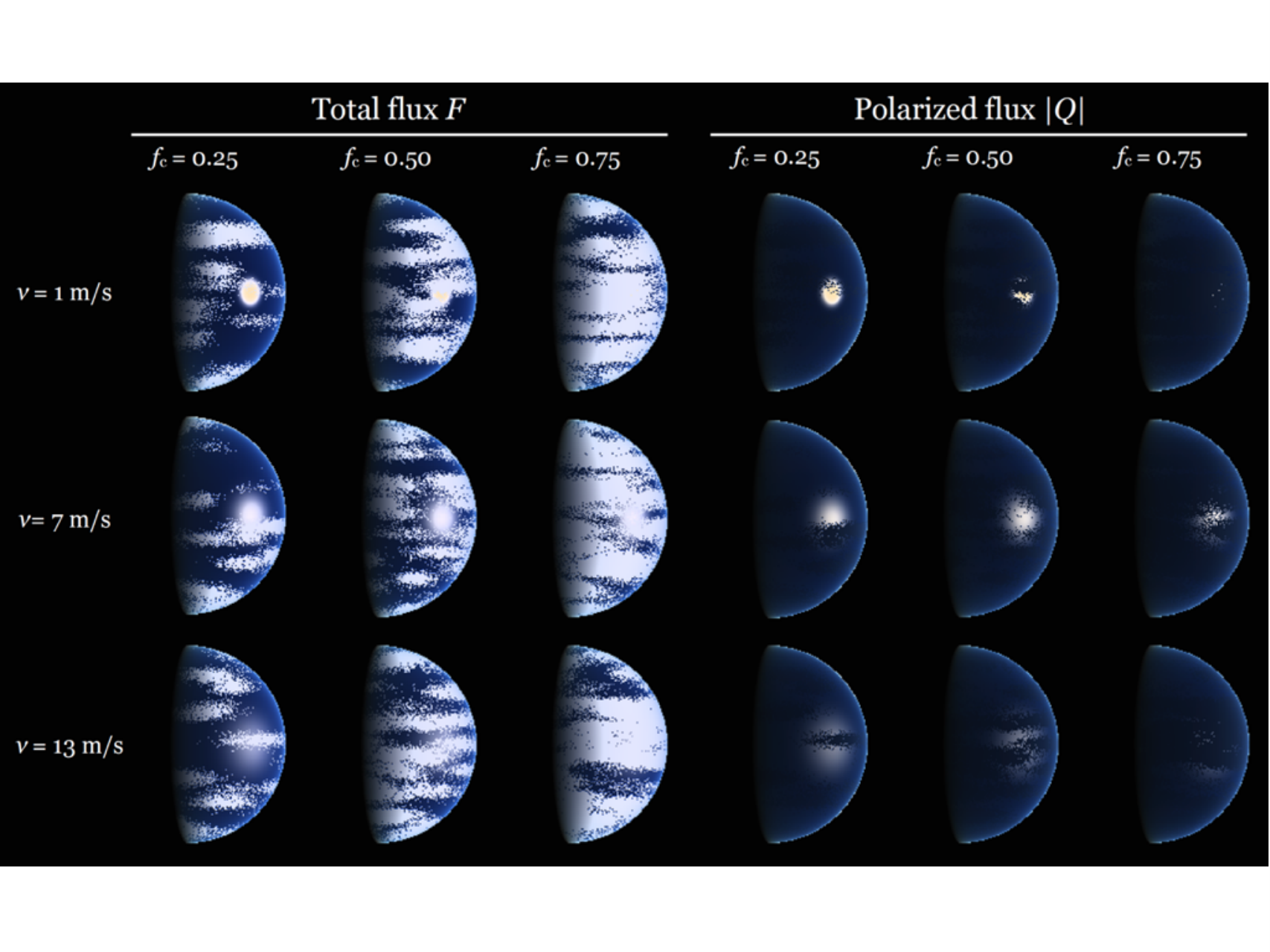
With patchy clouds, both the location and the cloud coverage fraction influences the reflected light signal (assuming for simplicity that the clouds are all the same and at the same altitude). Here, we show the influence of a horizontally inhomogeneous cloud deck on , , and of light reflected by an ocean planet. Like on Earth, our model cloud deck consists of patches of clouds, as described in Sect. 2.3.1 with a cloud coverage fraction . Figure 7 shows the disk-resolved RGB colors of the reflected and for model planets with different cloud coverage fractions and wind speeds (for every combination of and , the model planet has a different cloud pattern) at . The glint can be seen to appear between the clouds, and with increasing , the width of the glint pattern increases while its peak value decreases.
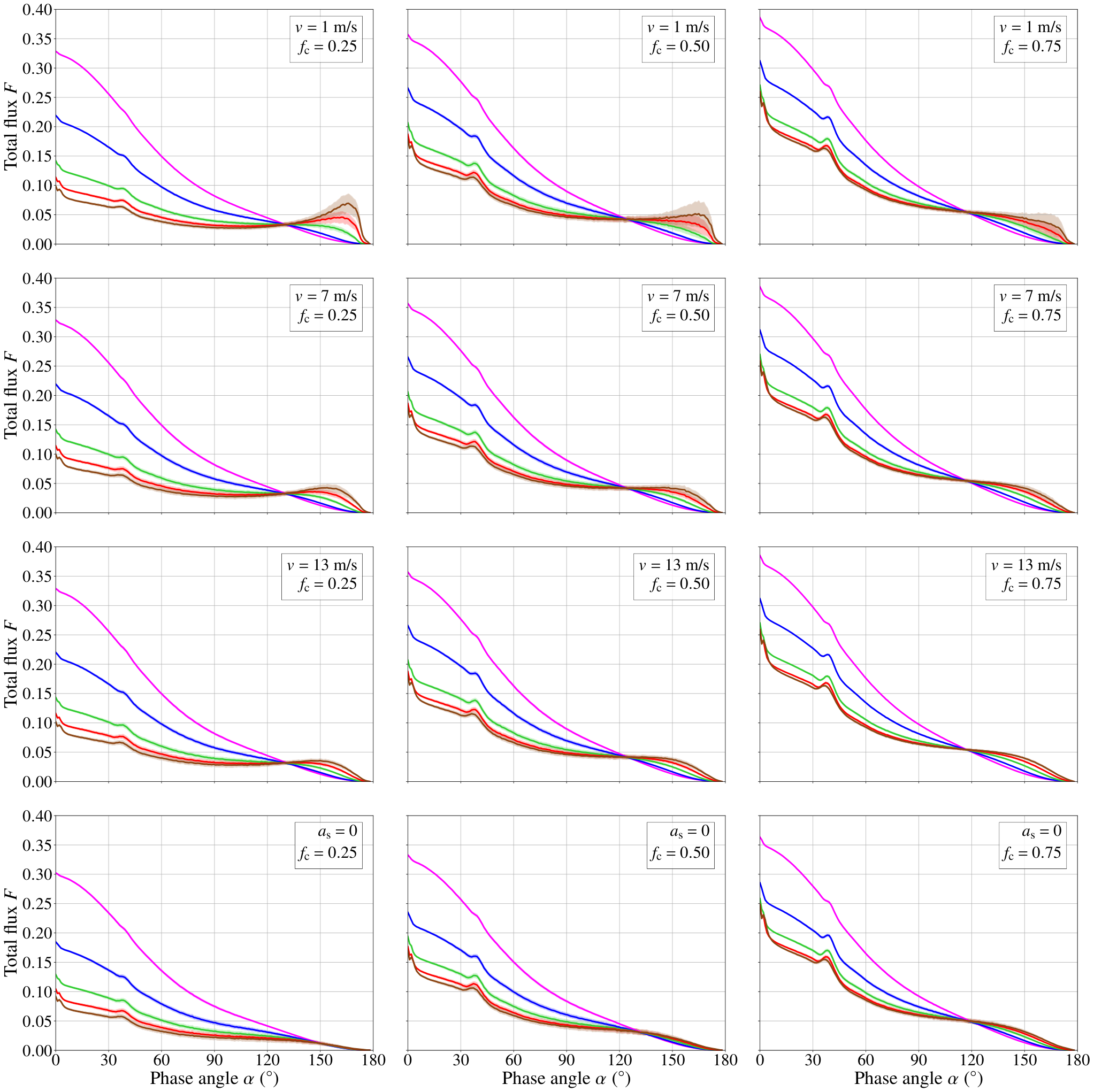
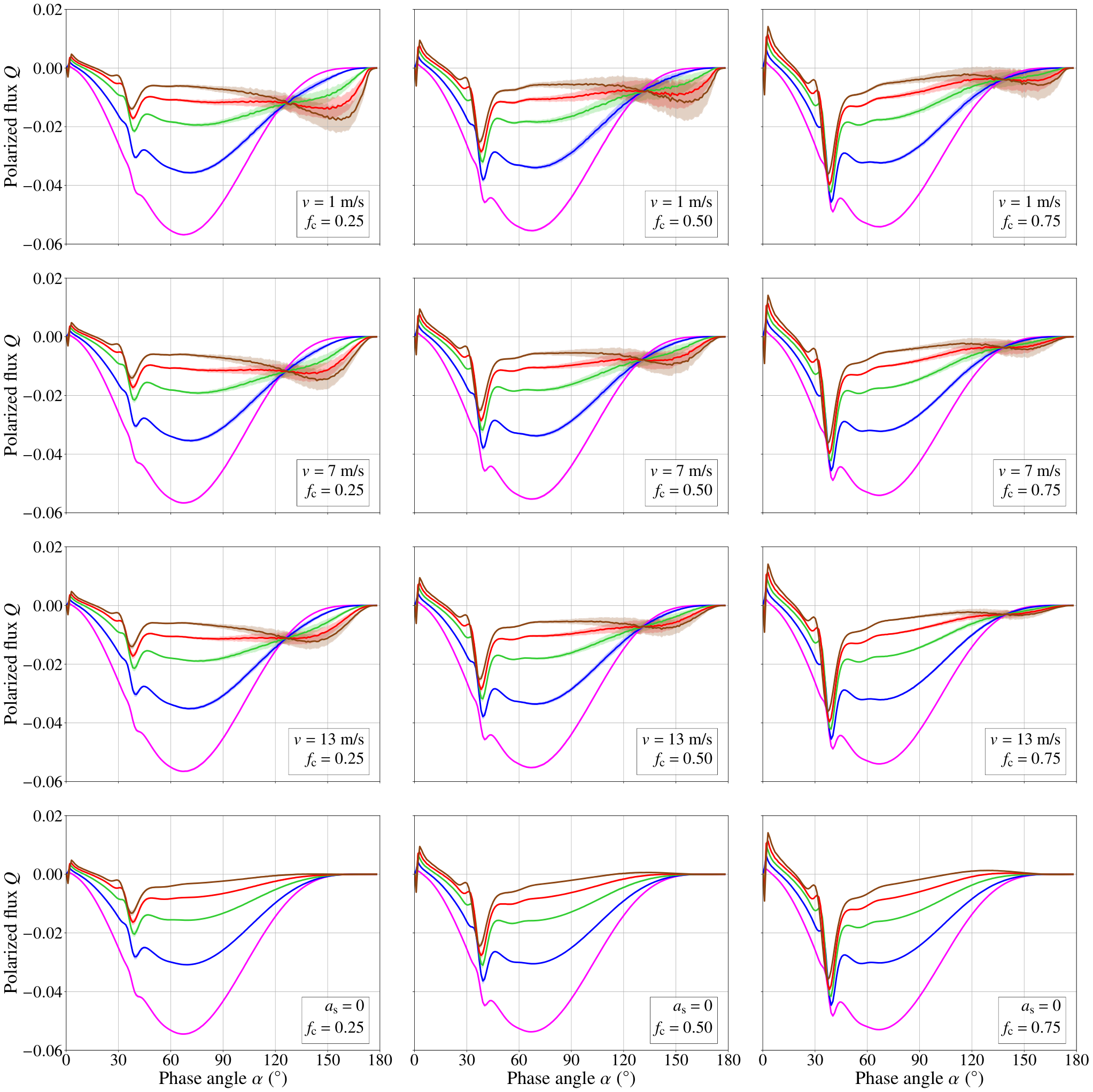
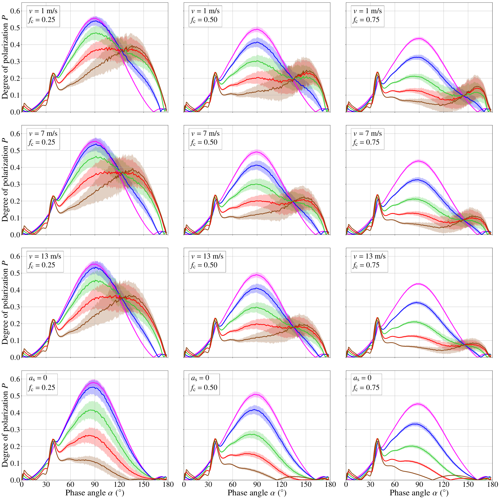
Figures 8-10 show , , and for the ocean planet for different values of and . Also included are the curves for a black surface planet beneath the clouds. We used 160 pixels across the equator, just like in Fig. 7. For every , we computed , , and (since planets with patchy clouds are usually not symmetric with respect to the reference plane) for 300 different patchy cloud patterns. The figures show the averages and the 1- standard deviation (the variability). Despite the non-symmetric cloud patterns, the disk-integrated linearly polarized flux appears to be smaller than 0.00003 for all model planets, across all phase angles. We thus do not show in the figures (even though it is very small, is included in the computation of ).
As can be seen in Fig. 8, total flux generally increases with increasing , and the curves for the ocean planet are somewhat higher than for the black surface planet. The influence of the variability of the cloud coverage for a given value of is small and only apparent at the longest wavelengths and the largest ’s. At the smallest wavelengths, the significant Rayleigh scattering above and between the clouds subdues the contrast between the bright clouds and the dark background, thus reducing the variability. At the largest phase angles, the surface area on the disk that provides the signal is smallest, and there is more variability in the coverage of cloudy pixels across that area ( is defined on the whole disk). A more in-depth discussion of the relation between and variability can be found in Rossi & Stam 2017.
Polarized flux generally decreases with increasing (Fig. 9), and is slightly larger for the ocean planet than for the black surface planet. The curves for the black surface planet show virtually no variability, while the variability in of the ocean planet is significant for the longer wavelengths and ’s larger than 90∘, in particular for small wind speeds.
Like the and phase curves of the cloud-free and completely cloudy ocean planets, the and phase curves of the ocean planets with patchy clouds for the different ’s cross each other at a given phase angle (see Figs. 8 and 9). Around that (which is different for and ), the planets thus appear white in total and polarized fluxes. The crossing is also present in for large cloud fractions () over a black surface planet, in agreement with the earlier results for completely cloudy black surface planets (Fig. 6). A black (or dark) surface planet with patchy clouds will, however, appear more whitish than red at the largest phase angles, because the spectral dispersion of is small.

Figure 10 shows the phase curves of the ocean and black surface planets with patchy clouds. The largest variation in is seen at the longest wavelengths, where the contribution of the gaseous atmosphere is smallest and the contribution of the surface is largest, and at intermediate to large ’s, where the contribution of the glint is strongest, and thus where the location of a cloud is relatively more important than at the smaller ’s (cf. Fig. 7). There appears to be little dependence of both the average curves and the variability in on wind speed , except for .
For ocean planets with patchy clouds, the curves of show crossings, i.e. the planet will show a color change, just like the curves for and . While this crossing in does not occur for the completely cloudy planet (), as was shown in Fig. 6, it does show up for (see Fig. 10). The black surface planet with patchy clouds does not show a color change. Measuring a color change in in the relevant phase angle range would thus indicate the presence of an ocean, even in the presence of patchy clouds.
Apart from the crossing in the phase curve for a cloudy ocean planet, there are more differences from the phase curve of the cloudy black surface planet. For example, Fig. 10 shows that for nm and both up to (at least) 0.50, the slope of for the ocean planet is positive between , while that for the black surface planet is negative. Additionally, the variability in is much larger for the ocean planet than for the black surface planet because of the appearance and disappearance of the polarized glint between the clouds.
Figure 11 shows the disk-resolved and of the ocean planet and the black surface planet with patchy clouds () at a range of phase angles to illustrate the reddening of both planets in and the reddening of the ocean planet in . It can also be seen that the glint makes the ocean planet somewhat lighter in blue than the black surface planet. In the images of the black surface planet at the largest phase angles the reddening of the planet in due to the clouds is visible. This cloud reddening also happens with the ocean planet, but there the reddening of the glint is more significant.
4 Discussion of the color change
Our results show that the presence of an exo-ocean could be revealed through a color change in the polarized flux of starlight that is reflected by a planet, except when the planet is completely covered by a thick cloud deck. The total reflected flux and degree of polarization can also show color changes. The crossing ’s, or ’s, where the color change takes place, are generally different for , , and , and depend on the cloud fraction .
An indication of such a crossing in measured phase curves of of sunlight that is reflected by the Earth, has recently been presented by Sterzik et al. 2019. They measured for ranging from to as derived from Earth-shine data obtained with ESO’s Very Large Telescopes in Chile. The phase angle range of these Earth-shine data is limited by the lunar phase during the observations77 7 Small phase angles of the Earth require observations at a large lunar phase angle, and thus with large background sky brightness, while large phase angles of Earth can only be done at small lunar phase angles, where the dark part of the lunar surface is relatively small., so unfortunately, the phase curves do not include the rainbow angle, which would have provided an interesting comparison with the strength of the rainbow in our simulations. In the Earth-shine measurements, appears to vary from about 120∘ to 135∘. The observations span a period of about two years and during the observations either South America and the Atlantic Ocean (east of Chile) were turned towards the moon or the Pacific Ocean (west of Chile) (Sterzik et al. 2019). The of about 135∘ was measured over the Pacific Ocean.
Figure 12 shows RGB color phase curves of and reflected by the ocean planet and the black surface planet for cloud fractions ranging from 0.0 to 1.0 in steps of 0.01. The phase curves for each wavelength are computed using so-called quasi horizontally inhomogeneous ocean planets, in the weighted sum approach as described by Stam 2008. In this approach, and of a horizontally inhomogeneous planet are computed by taking a weighted sum of the ’s and ’s computed for horizontally homogeneous planets with the atmosphere-surface combinations that occur on the inhomogeneous planet. Each weighting factor equals the fraction of the planetary disk that is covered by a given atmosphere-surface combination. A careful comparison (see App. C) shows that while the weighted sum approach does not directly provide variances due to the spatial distribution of cloud patches across the disk, it does indeed allow us to rapidly and accurately compute the average phase curves of , , and hence the respective values of ’s, using a small step size for . Fig. 12 illustrates that the color change in (i.e. where the RGB color changes from blue, through white, to red) is unique for ocean planets for up to 0.98. For , the crossing of the phase curves at the RGB wavelengths is too small to detect.
Figure 13 shows for , , and as functions of the cloud fraction , using the weighted sum approach. The of the inhomogeneous planet is computed from the summed total and ( of such a quasi horizontally inhomogeneous planet is always zero). The figure also includes ’s for the ocean planets as shown in Figs. 8 - 10, and thus computed for actual horizontally inhomogeneous planets. A comparison between these data points (the symbols) and the data computed assuming quasi horizontally inhomogeneous planets (the lines) in Fig. 13, shows that the weighted sum approach predicts with a maximum deviation of 0.35∘ (in for ). Also shown in Fig. 13, is computed for higher clouds (with a cloud top pressure, , of 0.5 bar) and optically thicker clouds (with = 10). Note that we did not include curves for planets with black surfaces in Fig. 13, because there are no color changes in and for such planets (cf. the bottom rows of Figs. 9 and 10), while the color change in is not very strong due to the small dispersion. The horizontal axis at the top indicates the minimum inclination angle orbital that is required to be able to observe an exoplanet at that particular phase angle; i.e. a color change expected to take place at can be observed if the inclination angle of the planetary orbit is at least 50∘.
Increasing the cloud coverage on an ocean planet decreases for the total flux , as can be seen in the figure, because more long wavelength light will be reflected at a given : ranges from for cloud-free planets () to for a fully cloudy planet (). Increasing the cloud top altitude for a given , increases , because the higher the clouds, the smaller the contribution of short wavelength (Rayleigh scattered) light at a given . An optically thicker cloud reflects more light, and will thus decrease in .
Increasing increases for the polarized flux , because more light will be reflected by the clouds, and less by the ocean at a given : ranges from for cloud-free planets () to , where the color change starts to disappear for an almost fully cloudy planet (). Increasing the cloud top altitude (i.e. decreasing ) at a given , increases because with higher clouds, a longer atmospheric path length, thus a more slanting incoming direction, is required for the short wavelength light to be sufficiently scattered out of the incident beam. Increasing the cloud optical thickness, , has virtually no effect on of , because a thicker cloud will add mostly unpolarized light to the reflected signal.
For the degree of polarization , Fig. 13 shows that increasing , increases . Indeed, the range of appears to be largest for : for as small as 0.03, , while for , the color change starts to disappear at (cf. Fig. 6). There is no crossing in for , which is consistent with our conclusion that a crossing in indicates an ocean that is partly covered by clouds: without clouds, there is no color change. Increasing the cloud top altitude, decreases for , while increasing the cloud optical thickness , increases slightly and only for .
The crossings in the phase curves of derived from Earth-shine measurements by Sterzik et al. 2019 occurred between about 120∘ to 135∘. Taking into account the order of magnitude of the variation in with the 1- standard deviation of the phase curve, the cloud coverage fraction would have ranged between 0.2 and 0.6. The later value pertains specifically to observations with the Pacific Ocean (west of Chile) turned towards the moon. Observations taken when South America and the Atlantic Ocean were turned towards the moon (east of Chile) would be influenced not only by the reflection by the ocean but also by South America. The influence of land surface reflection (albedo, reflection properties and coverage fraction) on will be part of a future study.
Finally, our model clouds consist of liquid water particles only, but on Earth, high altitude clouds can of course also contain ice particles. If these particles are flat and horizontally oriented, they will produce their own glint feature (Marshak et al. 2017; Bréon & Dubrulle 2004; Chepfer 1999; Noel & Chepfer 2004, examples from Earth-observations, are described in). Whether or not the polarization signature of the glint due to such (usually optically thin) ice clouds will mimic and/or influence that of a surface ocean should be part of a future study. In particular, the influence of bright surface areas, such as high planetary latitudes that could be covered by ice and/or snow, on the disk–integrated fluxes and polarization would be interesting to investigate further. Cowan et al. 2012 postulated that the larger relative contribution of light reflected by polar regions at a planet’s crescent phase (assuming the light equator coincides more or less with the planet’s true equator), could yield a false positive for the glint of light reflected by an ocean. However, unless such snow and ice covered surfaces are very clean, we would mostly expect an increase in total flux , not in and/or , and thus a decrease of . Such an increase in and decrease in would mainly happen at the longest wavelengths, and would thus not result in a color change in and/or and a false-positive exo-ocean detection.
5 Summary and outlook
We have presented computed total and (linearly) polarized fluxes, and , and the degree of (linear) polarization, , of starlight that is reflected by ocean planets, i.e. planets with a liquid ocean ruffled by the wind on their surfaces, with the aim of identifying observables for the presence of an ocean, by comparing their signals against those of so-called black surface planets, with the same atmosphere but with a black surface.88 8 For planets that are symmetric with respect to the reference plane of the polarized fluxes (the plane through the centers of the star, the planet and the observer) only the polarized flux will be non-zero. While planets with patchy clouds will usually not be symmetric with respect to the reference plane, the disk-integrated polarized flux appears to be very small and while it is included in the computation of , we do not explicitly discuss it. Below, we summarize and reflect on our results.
The total flux of light reflected by an ocean planet will be slightly larger than that of a black surface planet, up till phase angles of about 100∘. Across these phase angles, both ocean and black surface planets will appear blue, for every cloud coverage fraction . With increasing from about , the color of a black surface planet will change from blue to white, while that of an ocean planet will change from blue to white, then to red, and then back to white (but extremely dark) at the largest phase angles.
The crossing phase angle , i.e. the where the planet’s color changes from blue, through white, to red, increases with increasing surface pressure: at 1 bar, , while at 6 bar, . The phase angle where the cloud-free ocean planet changes back from red to white, decreases with increasing surface pressure . For increasing up from about 6 bars, the planet’s reddish phase fades and with that the difference between the ocean planet and the black surface planet starts to disappear.
Angle decreases with increasing : while for a cloud–free planet () and bar, , for a fully cloudy planet (), . Angle is insensitive to the wind speed over the ocean, although the strength of the color change does depend on : the smaller , and thus the lower the waves and the less whitecaps, the redder the ocean planet would appear.
The polarized flux of light reflected by an ocean planet shows a similar color change from blue, through white, to red with increasing as the total flux . Crucially, for , the color change does not occur for black surface planets, only for ocean planets, independent of the cloud coverage fraction . Detecting a color change in would thus indicate the presence of an ocean on the surface of a planet. Angle for increases with increasing . For , , while for almost completely cloudy planets (), the color change starts to disappear at . Also, the color change in remains strong at higher surface pressures, and is even still present (somewhat) at a surface pressure of 10 bar. Furthermore, for bar, the crossing angle is more or less independent of both . Angle also appears to be independent of , although, like with , the smaller , the redder the ocean planet would appear in .
For ocean planets with patchy clouds (), the variability of due to variation in the location of the clouds is, at each , much larger than a black surface planet with a similar value of , in particular at longer wavelengths. This variability is caused by the highly polarized glint appearing and disappearing from behind the patchy clouds.
The degree of polarization of light reflected by a cloud-free ocean planet is slightly lower at nm, 443 nm, and 550 nm compared to that of a cloud-free black surface planet, mostly due to the larger flux that is reflected by the ocean. Because the probability distribution of the slopes of the wave facets and the shadow function affect fluxes and in the same way, the dependence of on the wind speed is only due to the white cap distribution and scattering within the atmosphere, and thus relatively small. Indeed, for m/s, the maximum is about 5% smaller than for m/s at nm and using a whitecap albedo of 0.22. The phase angle where is maximum, increases from around to almost twice the Brewster angle of 106∘ with increasing , as the optical thickness of the atmosphere decreases and the contribution of the ocean to the reflected signal becomes more dominant. The location of the maximum , however, depends on the surface pressure . Indeed, an ocean-induced shift of the phase angle where is maximum towards larger values only occurs if is small (if is large, the presence of an ocean does not lead to a phase angle shift).
Like in , the variability in of an ocean planet, especially at the longer wavelengths and for all wind speeds, due to the glint appearing and disappearing from behind the clouds, would be much larger than the variability in of a black surface planet. A measurement of such variability could thus be used to identify an exo-ocean.
An ocean planet will change color in , but only if there are clouds. The color change phase angle strongly increases with , from about 88∘ for to about 161∘ for . Note that this range of is much broader than that for or , and it includes phase angles with a favorite planet-star separation. For , an ocean planet does not change color in . It would be interesting to investigate whether such low cloud fractions were to be expected in the presence of an ocean. The phase curves as derived from Earth-shine measurements by (Sterzik et al. 2019) show crossings that indicate cloud coverage fractions between 0.2 and 0.6.
While these cloud coverage fractions appear to be realistic for the Earth, the Earth-shine measurements covered a time period of several years, and two regions on Earth: the Pacific ocean (west of Chile) and the Atlantic ocean and South America (east of Chile). In addition, although Sterzik et al. 2019 took careful measures to correct their observations for the depolarizing reflection by the lunar surface, the Earth’s polarization phase functions might still include some unknown, and possibly wavelength dependent residual of the reflection by the moon, that could influence as derived from the curves. Indeed, flux and polarization measurements of sunlight that is reflected by the whole Earth, across the visible spectrum, covering our planet’s daily rotation and all phase angles, would allow the confirmation of using the color change of, in particular, for identifying the presence of an ocean. Such measurements (which would also show the rainbow feature that is not covered in the Earth-shine data) could be performed from the lunar surface or from a lunar orbiter (Karalidi et al. 2012b; Hoeijmakers et al. 2016, for measurement concepts, see).
Our simulations only include scattering by the atmospheric gas and by clouds consisting of liquid water droplets. Scattering and absorption by aerosol particles has not been included. Over the ocean, most aerosol particles are expected to be sea salt particles. Note that most of these aerosol particles will reside in the boundary layer, below the clouds. The influence of aerosols on the color change of a planet would depend on the aerosol column number density, and the aerosol microphysical properties, such as size, shape, and composition. The observation of the color change in in Earth-shine measurements by Sterzik et al. 2019 strongly suggests that the influence of aerosol particles will be minor, but a follow-up study with realistic ocean-type aerosols added to our atmosphere model, will give more insight into their role. In such a follow-up study, also the influence of oriented ice crystals can be investigated.
In our numerical simulations, we assume that the incident starlight is wavelength independent. This assumption is irrelevant for our results, as measured fluxes and could straightforwardly be normalized to the color of the incident stellar light99 9 By doing that, inelastic scattering processes, such as rotational Raman scattering, would be ignored, but this would only affect high spectral resolution features, such as absorption lines and Fraunhofer lines.. The degree of polarization is of course independent of any wavelength dependence of the incident stellar spectrum1010 10 Again, apart from high spectral resolution features due to e.g. rotational Raman scattering..
Our simulations provide yet another example of the value of polarimetry as a tool for exoplanet characterization: especially the detection of a color change of the polarized flux would uniquely identify a liquid surface ocean, and a color change in would indicate an ocean that is at least partly covered by clouds. The phase angle at which the color change in takes place depends on the cloud coverage fraction : for a cloud-free planet () and for an almost fully clouded planet () where the color change starts to disappear. The color change in takes place at phase angles from about for to for . Whether or not an exoplanet ever attains the phase angle at which a color change takes place, depends on the inclination angle of the planetary orbit, as can be seen in Fig. 13. A phase angle of 123∘ is attained along orbits with an inclination angle of at least 33∘, while for a phase angle of 161∘, the orbital inclination angle has to be at least 71∘. For intermediate cloud fractions, such as that on Earth, inclination angles larger than about 40∘ are required.
Current and near future space missions such as NASA’s TESS (Ricker et al. 2015) and ESA’s PLATO mission (Rauer et al. 2014) will provide transiting exoplanets, thus with close to 90∘, around bright, nearby stars. These planets will be excellent targets for searching for a color change in the polarized light signal. This color change can be measured at smaller phase angles, where the angular separation between the star and the planet is larger, than the glint, i.e. the increased reflected flux of starlight on the ocean surface, that was proposed as exo-ocean identifier by e.g. Williams & Gaidos 2008 and Robinson et al. 2010 (our Fig. 8 shows the glint in around for a wind speed of 1 m/s). Thus, using polarization to identify exo-oceans is not limited to crescent planetary phase angles.
We have shown that the color change in total flux can also occur with a zero surface albedo planet, with clouds below a Rayleigh scattering gas layer, while color changes in and only occur for the ocean planets. We have also shown that the lack of a color change in could mistakenly be interpreted as a negative for an exo-ocean in case of high surface pressures. The color change in remains present at high surface pressures (see Fig. 2). Furthermore, as shown by Cowan et al. 2012, the relative contribution of high planetary latitudes, which are more likely to be covered by ice and/or snow, to the disk-integrated fluxes increases with increasing phase angle towards the crescent phase, creating a false-positive detection of the glint. However, unless the ice is perfectly clean, we would not expect this increased contribution to yield a color change in and/or . Polarimetry would thus be a more robust tool against the false-positive identification of exo-oceans. Dedicated numerical simulations would be required to confirm this.
The crucial role that liquid water plays for life on Earth should spur feasibility studies into measuring the color change of an exoplanet in polarized flux and/or degree of polarization by future telescopes that are designed to measure starlight that is reflected by exoplanets. Apart from EPOL (Keller et al. 2010), the imaging polarimeter for EPICS, the Exoplanet Imaging Camera and Spectrograph for the European Extremely Large Telescope (Kasper et al. 2010), current space telescope concepts, such as LUVOIR (The LUVOIR Team 2018) and HabEx (Gaudi et al. 2018) do not include polarimetry across the visible,1111 11 LUVOIR does include POLLUX, a polarimeter at ultraviolet wavelengths (Bouret et al. 2018) and will thus not be able to measure the color changes.
While our numerical simulations pertain to the planet-signal only, and do not include any background starlight, the color change in polarized flux and/or degree of polarization could also be searched for in the combined light of the star and the planet. Obviously, of this combined light would be very small because of the added, mostly unpolarized stellar flux, but extracting this very small planet signal from the background stellar signal and noise could possibly be facilitated using the variation of along the planetary orbit, and the knowledge that the color change would be limited to the planetary signal.
Acknowledgements.
The authors thank Johan de Haan, Jacek Chowdhary, and Mike Zugger for sharing their knowledge and insights on the topic of this paper, and they thank the anonymous referee and the editor for their constructive comments.References
- Bailey (2007) Bailey, J. 2007, Astrobiology, 7, 320
- Berdyugina et al. (2011) Berdyugina, S. V., Berdyugin, A. V., Fluri, D. M., & Piirola, V. 2011, ApJ, 728, L6
- Bouret et al. (2018) Bouret, J.-C., Neiner, C., Gómez de Castro, A. I., et al. 2018, in Society of Photo-Optical Instrumentation Engineers (SPIE) Conference Series, Vol. 10699, Space Telescopes and Instrumentation 2018: Ultraviolet to Gamma Ray, 106993B
- Breón (1993) Breón, F. M. 1993, Remote Sensing of Environment, 43, 179
- Bréon & Dubrulle (2004) Bréon, F.-M. & Dubrulle, B. 2004, Journal of Atmospheric Sciences, 61, 2888
- Buenzli & Schmid (2009) Buenzli, E. & Schmid, H. M. 2009, A&A, 504, 259
- Chepfer (1999) Chepfer, H. 1999, J. Quant. Spec. Radiat. Transf., 63, 521
- Chowdhary (1999) Chowdhary, J. 1999, PhD thesis, Columbia University
- Chowdhary et al. (2006) Chowdhary, J., Cairns, B., & Travis, L. D. 2006, Applied Optics, 45, 5542
- Cotton et al. (2017) Cotton, D. V., Marshall, J. P., Bailey, J., et al. 2017, MNRAS, 467, 873
- Cowan et al. (2012) Cowan, N. B., Abbot, D. S., & Voigt, A. 2012, ApJ, 752, L3
- Cowan et al. (2009) Cowan, N. B., Agol, E., Meadows, V. S., et al. 2009, ApJ, 700, 915
- Cox & Munk (1954) Cox, C. & Munk, W. 1954, Journal of the Optical Society of America (1917-1983), 44, 838
- Cox & Munk (1956) Cox, C. & Munk, W. 1956, Slopes of the sea surface deduced from photographs of sun glitter, Bulletin of the Scripps Institution of Oceanography of the University of California (University of California Press & Cambridge University Press)
- de Haan et al. (1987) de Haan, J. F., Bosma, P. B., & Hovenier, J. W. 1987, AAP, 183, 371
- De Rooij & van der Stap (1984) De Rooij, W. A. & van der Stap, C. C. A. H. 1984, A&A, 131, 237
- Deming et al. (2013) Deming, D., Wilkins, A., McCullough, P., et al. 2013, ApJ, 774, 95
- Fraine et al. (2014) Fraine, J., Deming, D., Benneke, B., et al. 2014, Nature, 513, 526
- Garcia (2012a) Garcia, R. D. M. 2012a, Journal of Quantitative Spectroscopy and Radiative Transfer, 113, 306
- Garcia (2012b) Garcia, R. D. M. 2012b, Journal of Quantitative Spectroscopy and Radiative Transfer, 113, 2251
- García Muñoz (2015) García Muñoz, A. 2015, International Journal of Astrobiology, 14, 379
- Gaudi et al. (2018) Gaudi, B. S., Seager, S., Mennesson, B., et al. 2018, arXiv e-prints, arXiv:1809.09674
- Hale & Querry (1973) Hale, G. M. & Querry, M. R. 1973, Applied Optics, 12, 555
- Hansen & Hovenier (1974) Hansen, J. E. & Hovenier, J. W. 1974, Journal of Atmospheric Sciences, 31, 1137
- Hansen & Travis (1974) Hansen, J. E. & Travis, L. D. 1974, Space Science Reviews, 16, 527
- Hoeijmakers et al. (2016) Hoeijmakers, H. J., Arts, M. L. J., Snik, F., et al. 2016, Optics Express, 24, 21435
- Hovenier et al. (2004) Hovenier, J. W., van der Mee, C., & Domke, H. 2004, Transfer of Polarized Light in Planetary Atmospheres; Basic Concepts and Practical Methods (Kluwer, Dordrecht; Springer, Berlin)
- Hovenier & van der Mee (1983) Hovenier, J. W. & van der Mee, C. V. M. 1983, A&A, 128, 1
- Hsiung (1986) Hsiung, J. 1986, Journal of Geophysical Research, 91, 10,585
- Kaltenegger & Traub (2009) Kaltenegger, L. & Traub, W. A. 2009, ApJ, 698, 519
- Karalidi & Stam (2012) Karalidi, T. & Stam, D. M. 2012, A&A, 546, A56
- Karalidi et al. (2011) Karalidi, T., Stam, D. M., & Hovenier, J. W. 2011, A&A, 530, A69
- Karalidi et al. (2012a) Karalidi, T., Stam, D. M., & Hovenier, J. W. 2012a, A&A, 548, A90
- Karalidi et al. (2012b) Karalidi, T., Stam, D. M., Snik, F., et al. 2012b, Planet. Space Sci., 74, 202
- Kasper et al. (2010) Kasper, M., Beuzit, J.-L., Verinaud, C., et al. 2010, in Proc. SPIE, Vol. 7735, Ground-based and Airborne Instrumentation for Astronomy III, 77352E–77352E–9
- Keller et al. (2010) Keller, C. U., Schmid, H. M., Venema, L. B., et al. 2010, in Proc. SPIE, Vol. 7735, Ground-based and Airborne Instrumentation for Astronomy III, 77356G
- Kemp et al. (1987) Kemp, J. C., Henson, G. D., Steiner, C. T., & Powell, E. R. 1987, Nature, 326, 270
- Koepke (1984) Koepke, P. 1984, Applied Optics, 23, 1816
- Kostogryz et al. (2015) Kostogryz, N., Yakobchuk, T., & Berdyugina, S. 2015, ApJ, 806, 97
- Kreidberg et al. (2014) Kreidberg, L., Bean, J. L., Désert, J.-M., et al. 2014, ApJ, 793, L27
- Lustig-Yaeger et al. (2018) Lustig-Yaeger, J., Meadows, V. S., Tovar Mendoza, G., et al. 2018, ApJ, 156, 301
- Marshak et al. (2017) Marshak, A., Várnai, T., & Kostinski, A. 2017, Geochim. Res. Lett., 44, 5197
- Mishchenko et al. (2000) Mishchenko, M. I., Hovenier, J. W., & Travis, L. D. 2000, Light scattering by nonspherical particles : theory, measurements, and applications (Sand Diego: Academic Press)
- Mishchenko & Travis (1997) Mishchenko, M. I. & Travis, L. D. 1997, Journal of Geophysical Research, 102, No.D14:16989
- Monahan & Ó Muircheartaigh (1980) Monahan, E. C. & Ó Muircheartaigh, I. 1980, Journal of Physical Oceanography, 10, 2094
- Morel (1974) Morel, A. 1974, Optical Aspects of Oceanography, 1, 1
- Morel & Maritorena (2001) Morel, A. & Maritorena, S. 2001, Journal of Geophysics Research, 106, 7163
- Nakajima (1983) Nakajima, T. 1983, Journal of Quantitative Spectroscopy and Radiative Transfer, 29, 521
- Noel & Chepfer (2004) Noel, V. & Chepfer, H. 2004, Journal of Atmospheric Sciences, 61, 2073
- Oakley & Cash (2009) Oakley, P. H. H. & Cash, W. 2009, ApJ, 700, 1428
- Pope & Fry (1997) Pope, R. M. & Fry, E. S. 1997, Applied Optics, 36, 8710
- Rauer et al. (2014) Rauer, H., Catala, C., Aerts, C., et al. 2014, Experimental Astronomy, 38, 249
- Ricker et al. (2015) Ricker, G. R., Winn, J. N., Vanderspek, R., et al. 2015, Journal of Astronomical Telescopes, Instruments, and Systems, 1, 014003
- Robinson et al. (2010) Robinson, T. D., Meadows, V. S., & Crisp, D. 2010, ApJ, 721, L67
- Rossi et al. (2018) Rossi, L., Berzosa-Molina, J., & Stam, D. M. 2018, A&A, 616, A147
- Rossi & Stam (2017) Rossi, L. & Stam, D. M. 2017, A&A
- Rossi & Stam (2017) Rossi, L. & Stam, D. M. 2017, A&A, 607, A57
- Rossi & Stam (2018) Rossi, L. & Stam, D. M. 2018, A&A, 616, A117
- Sancer (1969) Sancer, M. 1969, IEEE Transactions on Antennas and Propagation, 17, 577
- Smith (1967) Smith, B. 1967, IEEE Transactions on Antennas and Propagation, 15, 668
- Smith & Baker (1981) Smith, R. C. & Baker, K. S. 1981, Applied Optics, 20, 177
- Sogandares & Fry (1997) Sogandares, F. M. & Fry, E. S. 1997, Applied Optics, 36, 8699
- Stam (2008) Stam, D. M. 2008, A&A, 482, 989
- Stam et al. (2006) Stam, D. M., de Rooij, W. A., Cornet, G., & Hovenier, J. W. 2006, A&A, 452, 669
- Stam & Hovenier (2005) Stam, D. M. & Hovenier, J. W. 2005, A&A, 444, 275
- Sterzik et al. (2019) Sterzik, M. F., Bagnulo, S., Stam, D. M., Emde, C., & Manev, M. 2019, A&A, 662, A41
- Sun & Lukashin (2013) Sun, W. & Lukashin, C. 2013, Atmospheric Chemistry & Physics, 13, 10303
- Talens et al. (2017) Talens, G. J. J., Spronck, J. F. P., Lesage, A. L., et al. 2017, A&A, 601, A11
- The LUVOIR Team (2018) The LUVOIR Team. 2018, arXiv e-prints, arXiv:1809.09668
- Tinetti et al. (2007) Tinetti, G., Vidal-Madjar, A., Liang, M.-C., et al. 2007, Nature, 448, 169
- Tsang et al. (1985) Tsang, L., Kong, J. A., & Shin, R. T. 1985, Theory of microwave remote sensing (New York: Wiley Interscience)
- Wiktorowicz & Stam (2015) Wiktorowicz, S. J. & Stam, D. M. 2015, Exoplanets, ed. L. Kolokolova, J. Hough, & A.-C. Levasseur-Regourd, 439
- Williams & Gaidos (2008) Williams, D. M. & Gaidos, E. 2008, Icarus, 195, 927
- Xu et al. (2016) Xu, F., Dubovik, O., Zhai, P.-W., et al. 2016, Atmospheric Measurement Techniques, 9, 2877
- Zhai et al. (2010) Zhai, P.-W., Hu, Y., Chowdhary, J., et al. 2010, Journal of Quantitative Spectroscopy and Radiative Transfer, 111, 1025
- Zhai et al. (2012) Zhai, P.-W., Kattawar, G. W., & Hu, Y. 2012, Journal of Quantitative Spectroscopy and Radiative Transfer, 113, 1981
- Zugger et al. (2010) Zugger, M. E., Kasting, J. F., Williams, D. M., Kane, T. J., & Philbrick, C. R. 2010, ApJ, 723, 1168
- Zugger et al. (2011a) Zugger, M. E., Kasting, J. F., Williams, D. M., Kane, T. J., & Philbrick, C. R. 2011a, ApJ, 739, 55
- Zugger et al. (2011b) Zugger, M. E., Kasting, J. F., Williams, D. M., Kane, T. J., & Philbrick, C. R. 2011b, ApJ, 739, 12
Appendix A The reflection matrix of the ocean
Because we fully include the polarization of light, we describe scattering, reflection and transmission processes by matrices1212 12 When ignoring circular polarization, the matrices will be . instead of by scalars. The reflection of light by a gas-liquid interface (in our case, an air-liquid water interface), with waves shaped by randomly oriented, flat facets, is described by the following matrix (Mishchenko & Travis 1997; Zhai et al. 2010, see)
| (5) | |||||
with the matrix describing the Fresnel reflection by a flat wave facet, with and the refractive indices of air and water, respectively (see Zhai et al. 2010, Eq. 47). In Eq. 5, , , , and , with , , , and the angles between the local zenith direction and the direction of propagation of the reflected light, the incident light (not only the direct beam but also the diffuse incident light), the normal on the wave facet, and the Fresnel reflection angle, respectively.
The matrices are rotation matrices that are used to rotate the reference plane for the incident light (through the local zenith direction and the direction of incidence) to the reference plane for the reflection by the wave facet (through the local normal on the facet, and the directions of incidence and reflection), and next to the reference plane of the reflected light (through the local zenith direction and the direction of reflection) (Hovenier & van der Mee 1983, see), given by
| (6) |
with the angle between the two reference planes, measured rotating in the anti-clockwise direction from the old to the new reference plane when looking in the direction of propagation (thus clockwise for an observer that looks towards the planet) (). The first rotation in Eq. 5 is over angle and the second rotation over angle .
Furthermore in Eq. 5, is the probability density function of the wave facet inclination angles, as follows (Breón 1993; Zhai et al. 2010, see)
| (7) |
The variance of the slopes of the wave facets, , depends on the wind speed (in m/s) and is given by (Cox & Munk 1954, see)
| (8) |
A larger wind speed thus increases the variance in the slopes.
in Eq. 5 describes the shadowing, i.e. the blockage of incident light and reflected light due to inclined wave facets. For this function we use (Smith 1967; Sancer 1969, see)
| (9) |
where
Here, is the complementary error function.
Part of the light that is incident on the Fresnel reflecting interface will be transmitted into the liquid ocean. Once in the ocean, this light can be scattered, or absorbed, or it can be absorbed by the black surface that we assume below the water body. The transmission of incident light from above (the star/sun or the sky) through the rough interface into the water, is described by the following transmission matrix:
| (10) | |||||
where , with the transmission angle at the wave facet, and is the Fresnel transmission matrix for a flat interface. Note that contains a factor to account for the changing solid angle of the light beam as it is transmitted through the air-water interface and for the changing flux because of the different permittivity of water compared to that of air (Zhai et al. 2010, see Eq. 48 of). The interface reflection and transmission matrices for illumination from below, and , respectively, may readily be derived following a similar approach (Zhai et al. 2010, see).
The matrix describing the reflection by the water below the interface, , is computed using the adding-doubling algorithm (see Sect. 2.3.2). The water body is bounded below by a black surface (the algorithm can also handle non-black surfaces, for example, when modeling reflection by shallow waters above lightly colored sand).
We compute the reflection matrix, , of the ’clean’ ocean body as a whole, i.e. of the rough interface and the water body, but without white caps, according to (Xu et al. 2016)
| (11) | |||
| (12) | |||
| (13) | |||
| (14) | |||
| (15) | |||
| (16) | |||
| (17) |
where , , and are rectangular super-matrices (see Sect. 2.3.2) and describes the reflection by the sub-interface water body (including the reflections between the water body and the interface).
Finally, we compute , the reflection matrix of the entire ocean (interface plus water body plus black surface below the water), and including white caps as follows (Koepke 1984; Sun & Lukashin 2013)
| (18) |
where is the matrix describing the Lambertian reflection by the white caps with a foam albedo and is the fraction of white caps as determined by the empirical relation of Monahan & Ó Muircheartaigh 1980
| (19) |
The influence of the white caps and the white cap albedo will be discussed in Appendix B.
Appendix B The reflection by white caps
Wind blowing across an ocean generates waves on the surface and with that, white caps or foam. The reflection matrix of the ocean as a whole (interface, water body, surface below the water) is computed using a weighted sum of the reflection matrix of the ocean without white caps, with its surface described by wave facets reflecting as Fresnel surfaces, and the reflection matrix of the white caps (see Eq. 18).
The reflection by the white caps or foam is assumed to be Lambertian, thus isotropic and non-polarizing, and the surface that is covered by white caps is flat. As baseline, we assume an effective foam albedo, , of 0.22, as empirically derived by Koepke 1984. Figure 14 shows the total and polarized fluxes and the degree of polarization of the ocean planet at 865 nm, for a wind speed of 7 m/s and our standard whitecap albedo of 0.22, for m/s and , for m/s and (the latter value is based on the uncertainty in the foam albedo value proposed by Koepke 1984), and for m/s and no whitecaps. The curves clearly show that the effect of the whitecap reflection is very small when m/s, as only 0.0003% of the surface is covered by whitecaps; the Lambertian reflection by the foam only slightly ( 1%) decreases the maximum as compared to the case without whitecaps. For m/s, the whitecaps cover 2.46% of the surface, and decrease the maximum by about 5 and 10% for and 0.33, respectively. The whitecaps shift the maximum from to about 103∘ and 108∘, respectively. We conclude that the smaller at m/s for = 865 nm in Fig. 4, compared to at m/s, is indeed caused by the whitecaps.
If white caps are ignored ( in Eq. 18), the degree of polarization of light that is reflected by the ocean is independent of the wind speed . The reason is that both the shadow function and the probability density function for the wave facet inclination angles , that depend on (see Eqs. 5-10), influence all elements of the ocean’s reflection matrix (and, if , matrix ) equally. The degree of polarization of an ocean planet as a whole can, however, depend (slightly) on , because when is large enough such that white caps cannot be ignored, light that is reflected by the foam and that is subsequently scattered within the atmosphere, will influence the total and polarized fluxes, and hence of the light that emerges from the top of the atmosphere.
Appendix C Horizontally inhomogeneous planets and the weighted sum approach
A fast way to estimate the average flux and polarization phase curves of a partly cloudy planet, for any cloud coverage fraction , is to compute the weighted sum of horizontally homogeneous planets (Stam 2008). That is, the total and polarized fluxes of a partly cloudy planet are derived from the respective total and polarized fluxes of a completely cloudy planet, , and a cloud-free planet, , according to
| (20) |
Because and have to be computed only once, Eq. 20 can be evaluated very fast for arbitrary cloud coverage fractions .
When using a weighted sum, the locations of cloud patches on a planet are not taken into account, while the locations can influence the total and polarized fluxes, and hence . In this appendix, we compare results of Eq. 20 to the average phase curves of planets with various distributions of horizontally inhomogeneous patchy clouds (for which the locations of the patches are thus fully accounted for) (see Sect. 3.2.2).
Figure 15 shows that the average phase curves of , , and for partly cloudy ocean planets with randomly distributed cloud patterns follow the phase curves computed using the weighted sum very accurately. For the curves in this figure, the wind speed is 7 m/s and the cloud coverage fraction 0.50. However, we find that for any combination of (1 m/s, 7 m/s, or 13 m/s) and (0.25, 0.50, or 0.75) the agreement between the average phase curves and the weighted sums is excellent.
It should be emphasized that we use random patchy cloud cover patterns. Hence, in the case of a planet with a non-random cloud pattern, e.g. a cloud pattern that is correlated to underlying continents, horizontally inhomogeneous planet models as presented in this paper may be needed to accurately model measured phase curves. In addition, using a weighted sum of horizontally homogeneous planets to compute phase curves of horizontally inhomogeneous planets does not provide information about the variability in the phase curves that is due to the variability in the cloud pattern, as shown by the shaded areas around the phase curves in Figs. 8-10.