A Framework to Control Functional Connectivity in the Human Brain

The structural (i.e., matrix of anatomical connections between brain regions) and functional (i.e., matrix of correlation coefficients between the activity of brain regions) connectivity of the brain vary across healthy individuals and those affected by neurological or psychiatric disorders, and can be used as biomarkers to detect or predict pathological conditions. While structural connectivity changes rather slowly over time and can be measured accurately via diffusion imaging techniques [1], functional connectivity depends on the instantaneous neural activity and is affected, for instance, by the tasks being performed and external stimuli [2]. Today, common measures of functional connectivity rely on resting-state functional magnetic resonance imaging (rs-fMRI) timeseries to quantify the level of correlated activity between brain regions. The relationships between structural and functional connectivity have recently received considerable attention [3, 4], and the tantalizing idea of controlling functional states by leveraging or modifying brain structure has given birth to a new, thrilling, field of research [5, 6, 7].

In this paper, we leverage the connection between structural and functional connectivity, and propose a framework to control functional connectivity by selectively modifying structural connectivity and the regions’ intrinsic frequencies (see Fig. 1). In particular, building on prior studies [8, 9], we model the brain’s neural activity as the phases of a collection of interconnected Kuramoto oscillators, and postulate that the level of functional connection between two regions is proportional to the level of synchronization between the phases of the oscillators associated with the two regions. Then, we derive conditions and methods to tune the oscillators’ interconnection weights and natural frequencies so as to enforce arbitrary synchronization patterns and, consequently, brain-wide functional connectivity. We remark that the control mechanisms used in our framework are biologically plausible. For instance, changes in the spontaneous neural activity (i.e., oscillators’ frequencies) are typical of the brain, involve natural modifications in regional metabolism of the neurons, and can alternatively be induced by a number of non-invasive stimulation techniques [10]. Changes to the structural interconnections (i.e., oscillators’ interconnections), instead, can arise from different chemical or electrical mechanisms including, at the microscale, Hebbian plasticity [11] and short-term synaptic facilitation [12].

At the core of our framework to model and control functional connectivity is the concept of cluster synchronization in a network of oscillators, where groups of oscillators behave cohesively but independently from other clusters. For the case of oscillators with Kuramoto dynamics as used in this work, [19, 20] explore approximate notions of cluster synchronization in simplified configurations, while [21] provides exact invariance conditions for arbitrary cluster synchronization manifolds. Our recent work introduces rigorous [22] and approximate [23] stability conditions for cluster synchronization, which are also used here. Compared to the above references, this paper focuses on the control of cluster synchronization, rather than on its enabling conditions.

On the application side, this work contains the first mathematically rigorous and neurologically plausible framework to control functional connectivity in the brain, and takes a significant step to fill the gap between empirical studies on oscillatory neural activity [8, 24, 9] and the recent technical body of work inspired by neural synchronization [19, 21, 22, 23]. In Section V, we apply our control technique to an empirically-reconstructed structural brain network, and validate our results by computing the correlation of resting-state fMRI signals obtained through a realistic hemodynamic model. As a minor contribution, our work extends [9] by allowing heterogeneous Kuramoto dynamics.

The aim of this work is to control network parameters so that groups of brain regions exhibit a high degree of functional connectivity. In this context, functional interactions are defined as the pairwise correlation between hemodynamic signals recorded in two brain regions. One model used to simulate such hemodynamic signals is described by a set of nonlinear differential equations [25] that can be approximated in the frequency domain as a linear low-pass filter [9]. Because the only input to such hemodynamic model is the oscillatory neural activity, the formation of strongly (functionally) connected brain regions can be promoted by controlling the synchronization level of their neural dynamics. We follow [9] to model such neural dynamics with a sparse network of heterogeneous Kuramoto oscillators that are connected to each other according to the anatomical architecture of the human brain, more specifically known as white matter tracts.¹¹ 1 We assume that at each node of a structural brain network there exists a community of excitatory and inhibitory neurons whose dynamical state is in a regime of self-sustained oscillation. In other words, the neurons’ firing rates delineate a limit cycle, and their dynamics can be approximated by a single variable, which is the angle (or phase) on this cycle. Ultimately, the problem of generating desired patterns of functional connectivity reduces to the one of controlling cluster synchronization in a network of heterogeneous Kuramoto oscillators.

To be precise, let $\mathcal{G}=(\mathcal{V},\mathcal{E})$ be a weighted digraph, where $\mathcal{V}=\{1,\dots,n\}$ and $\mathcal{E}\subseteq\mathcal{V}\times\mathcal{V}$ represent the oscillators, or nodes, and their interconnection edges, respectively. The $i$-th oscillator’s dynamics reads as:

where $\omega_{i}\in\mathbb{R}_{>0}$ denotes the natural frequency of the $i$-th oscillator, $\theta_{i}\in\mathbb{S}^{1}$ is its phase, $a_{ij}\in\mathbb{R}_{>0}$ is the weight of the edge $(j,i)\in\mathcal{E}$, with $a_{ij}=0$ when $(j,i)\not\in\mathcal{E}$, and $A=[a_{ij}]$ is the weighted adjacency matrix of $\mathcal{G}$.

To characterize synchronized trajectories among subsets of oscillators, let $\mathcal{P}=\{\mathcal{P}_{1},\dots,\mathcal{P}_{m}\}$ be a nontrivial partition of $\mathcal{V}$, where each cluster contains at least two oscillators and its graph is strongly connected.²² 2 As the brain is densely connected [26], this assumption is not restrictive. We say that a network exhibits cluster synchronization when the oscillators can be partitioned so that the phases of the oscillators in each cluster evolve identically. Formally, we define the cluster synchronization manifold associated with the partition $\mathcal{P}$ as

Then, the network is cluster-synchronized with partition $\mathcal{P}$ when the phases of the oscillators belong to $\mathcal{S}_{\mathcal{P}}$ at all times. Without loss of generality, the oscillators are labeled so that $\mathcal{P}_{k}=\{\sum_{\ell=1}^{k-1}|\mathcal{P}_{\ell}|+1,\dots,\sum_{\ell=1}^{k}|\mathcal{P}_{\ell}|\}$, where $|\mathcal{P}_{\ell}|$ denotes the cardinality of the set $\mathcal{P}_{\ell}$.

Because our control framework leverages conditions for the invariance and stability of the cluster synchronization manifold to modify the network weights and oscillators’ natural frequencies, we briefly recall useful preliminary results that have recently been established in [21, 22, 23]. Specifically, given a desired network partition $\mathcal{P}=\{\mathcal{P}_{1},\dots,\mathcal{P}_{m}\}$, invariance of $\mathcal{S}_{\mathcal{P}}$ is guaranteed by the following conditions:

• (C1)

  The natural frequencies satisfy $\omega_{i}=\omega_{j}$ for every $i,j\in\mathcal{P}_{k}$ and $k~\in~\{1,\dots,m\}$. Equivalently, $B_{\text{span}}^{\mathsf{T}}\omega=0$,

where $B_{\text{span}}\in\mathbb{R}^{|\mathcal{V}|\times|\bigcup_{k}\mathcal{E}_{\text{span},k}|}$ is the incidence matrix of $\bigcup_{k=1}^{m}\mathcal{T}_{k}$, with $\mathcal{T}_{k}=(\mathcal{P}_{k},\mathcal{E}_{\text{span},k})$ being a spanning tree of the digraph $\mathcal{G}_{k}$ of the isolated cluster $\mathcal{P}_{k}$;

• (C2)

  The network weights satisfy $\bar{V}_{\mathcal{P}}^{\mathsf{T}}\bar{A}V_{\mathcal{P}}=0$,

where $V_{\mathcal{P}}\in\mathbb{R}^{n\times m}$ is the characteristic matrix of the network defined as $V_{\mathcal{P}}=\left[{v_{1}}/{\|v_{1}\|},\dots,{v_{m}}/{\|v_{m}\|}\right]$, with

$\bar{V}_{\mathcal{P}}\in\mathbb{R}^{n\times(n-m)}$ is an orthonormal basis of the orthogonal subspace to the image of $V_{\mathcal{P}}$, and $\bar{A}=A-A\circ V_{\mathcal{P}}V_{\mathcal{P}}^{\mathsf{T}}$ is the matrix of inter-cluster connections only (see also [21]).

We assume that the isolated clusters are locally stable:

• (A$1$)

  The dynamics (1), with $a_{ij}=0$ when $i,j$ belong to different clusters, converges exponentially fast to $\mathcal{S}_{\mathcal{P}}$.

Notice that Assumption (A$1$) is satisfied when $\mathcal{G}_{k}$ has symmetric weights and condition (C$1$) holds [22, Lemma 3.1][27, Theorem 5.1]. In our case, (A$1$) is not restrictive because structural brain networks are typically symmetric [5].³³ 3 In a general case, one can ensure that Assumption (A$1$) is satisfied simply by pairing the control mechanism developed in the next session with an independent one that makes intra-cluster connections symmetric.

Let $\omega^{(k\ell)}$ denote the natural frequency difference between any two nodes in disjoint clusters $\mathcal{P}_{k}$ and $\mathcal{P}_{\ell}$. If (C$1$) and (C$2$) hold, then a tight approximate condition for $\mathcal{S}_{\mathcal{P}}$ to be locally exponentially stable is [23]:

• (C3)

  The natural frequencies and the network weights are such that $\lambda_{\text{max}}(\Xi(A,\omega))<1$, with $\Xi=[\xi_{k\ell}]$ and

where $G_{k}(s)=(sI-J_{k})^{-1}$, $J_{k}$ is the Hurwitz stable Jacobian matrix of the intra-cluster phase difference dynamics and $\nu_{k\ell}$ is a function of the inter-cluster weights. Due to space constraints, we refer the interested reader to [21, 23] for a detailed discussion on conditions (C1), (C2), and (C3).

In this section, we propose a control mechanism to obtain a prescribed and robust configuration of synchronized oscillatory patterns. Towards this aim, we consider a network $\mathcal{G}=(\mathcal{V},\mathcal{E})$ and an arbitrary partition $\mathcal{P}=\{\mathcal{P}_{1},\dots,\mathcal{P}_{m}\}$ of $\mathcal{V}$. The proposed control technique is minimally invasive in the sense that it looks for the smallest correction (in the Frobenius norm sense) of inter-cluster network weights and oscillators’ natural frequencies that renders the cluster synchronization manifold $\mathcal{S}_{\mathcal{P}}$ invariant and locally stable. In practice, a modification of the network parameters will require either the exploitation of neural plasticity or localized surgical intervention for the modification of the network weights and structure, and pharmacological or electromagnetic influence for the refinement of the brain regions’ natural frequencies. In mathematical terms, the approach is encoded into solving the following constrained minimization problem:

where $\Delta$ is the correction of the network matrix, $\mu$ is the correction of the natural frequencies vector, and the $(i,j)$-th entry of $\Delta$ is zero if $i$, $j$ belong to the same partition $\mathcal{P}_{k}$, $k\in\{1,\dots,m\}$. Further, $H$ is the $0$-$1$ adjacency matrix of $\mathcal{H}=(\mathcal{V},\mathcal{E}_{\mathcal{H}})$, which is the graph encoding the set of edges $\mathcal{E}_{\mathcal{H}}\subseteq\mathcal{E}$ that is allowed to be modified, and $H^{\text{c}}=\mathds{1}\mathds{1}^{\mathsf{T}}-H$. That is, the $(i,j)$-th entry of a solution $\Delta^{*}$ to problem (3) is zero when the corresponding $(i,j)$-th entry of $H$ is zero. The optimization problem (3) is illustrated in Fig. 2.

Constraints (3a) and (3b) are equivalent to conditions (C$2$) and (C$1$), respectively, for the invariance of $\mathcal{S}_{\mathcal{P}}$. Constraint (3c) restricts the corrective action to a subset of all the possible interconnections, in affinity with the practical limitations of localized interventions. Constraints (3d) and (3e) are due to biological compatibility and require the inter-cluster weights of the perturbed network and oscillators’ natural frequencies to be nonnegative. Finally, Constraint (3f) corresponds to (C3) and guarantees the (local) stability of $\mathcal{S}_{\mathcal{P}}$. In particular, the latter constraint makes the above problem non-convex and, therefore, potentially intractable from a numerical viewpoint. To overcome this issue, we next propose a suboptimal, yet numerically more tractable, control strategy. Specifically, we decouple (3) into two simpler subproblems. The first one solves for the smallest correction of inter-cluster weights satisfying (3a), (3c), and (3d), whereas the second one solves for the smallest correction of the oscillators’ natural frequencies satisfying (3b), (3e) and (3f).

In this section, we show that the control framework described in Section III, and in fact the stability property of the cluster synchronization manifold $\mathcal{S}_{\mathcal{P}}$, is robust to perturbations of the network parameters. That is, small changes in the oscillators’ natural frequencies and network weights yield a small deviation from cluster-synchronized trajectories. In light of this, the proposed control mechanism lends itself to practical applications, where the network parameters are not known exactly and the neural dynamics is subject to noise.

Consider the dynamics (1) with perturbed parameters:

where $\tilde{\omega}_{i}=\omega_{i}+\delta\omega_{i}$ and $\tilde{a}_{ij}=a_{ij}+\delta a_{ij}$. Notice that, if $\delta\omega_{i}=0$ and $\delta a_{ij}=0$, the dynamics (8) is equivalent to (1). From (8), the perturbed intra-cluster difference dynamics of nodes $i,j\in\mathcal{P}_{k}$, with $k\in\{1,\dots,m\}$, reads as:

where $\delta_{ij}=\delta\omega_{j}-\delta\omega_{i}+\sum_{z=1}^{n}[\delta a_{jz}\sin(\theta_{z}-\theta_{j})$ $-\delta a_{iz}\sin(\theta_{z}-\theta_{i})]$. Finally, let $\delta$ be the vector of all $\delta_{ij}$ that affect the nominal intra-cluster dynamics as in (IV).

We are now ready to present the main result of this section, which resorts to the prescriptive stability condition derived in [22] that we recall in the Appendix B for completeness.

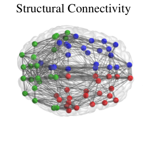
We conclude this paper with the application of the control mechanism presented in Section III to the brain network estimated in [1], which is publicly available at http://umcd.humanconnectomeproject.org/umcd. In these data, structural connectivity is proportional to large-scale connection pathways between cortical regions, and the gray matter is subdivided into $n=66$ cortical regions ($33$ per hemisphere). To show the effectiveness of our proposed method in enforcing desired functional connectivity by means of arbitrary synchronization patterns, we partition the structural brain network in $3$ clusters, i.e. $\mathcal{P}=\{\mathcal{P}_{1},\mathcal{P}_{2},\mathcal{P}_{3}\}$, each one comprising $22$ regions that do not belong to any known functionally connected resting-state network. The three clusters are highlighted with different colors in Fig. 3 and Fig. 3. Furthermore, following our goal of providing a method to enhance the synchronization properties of a diseased or damaged brain, we simulate the effects of brain damage, e.g., a stroke, by damping the connectivity of one cluster [31]. That is, we weaken the intra-cluster connections of the first cluster by a scaling factor $10^{-2}$ to echo reduced structural connectivity, and we show that our technique can in fact recover stability of the cluster synchronization manifold associated with the desired network partition.⁶⁶ 6 Specifically, weakening the intra-cluster connections of one cluster is likely to make $\mathcal{S}_{\mathcal{P}}$ unstable [23].

Before presenting our results, we describe the methodology used to simulate human rs-fMRI functional connectivity.

In this work, we propose a minimally invasive technique to obtain robust synchronization patterns in sparse networks of heterogeneous Kuramoto oscillators. To the best of our knowledge, this is the first attempt at blending mathematically rigorous methods with physiological models of brain activity with the goal of steering whole-brain synchronization dynamics. Specifically, we cast a constrained optimization problem whose solution not only satisfies mathematical conditions for invariance and stability of an arbitrary cluster synchronization manifold, but also meets biological constraints. We decompose the complete optimization problem into two simpler subproblems, and provide efficient methods to solve them. When applying our technique to correct the network parameters of empirically-reconstructed anatomical brain data, we find that our solution, although suboptimal, provides a result that is well within the range of physiologically plausible parameters. Additionally, we show that cluster synchronization is robust to small parameter mismatches and numerical inaccuracies. This result complements previous prescriptive studies on cluster synchronization and enables the use of our framework in practical situations.

References

- [1] P. Hagmann, L. Cammoun, X. Gigandet, R. Meuli, C. J Honey, V. J Wedeen, and O. Sporns. Mapping the structural core of human cerebral cortex. PLoS Biology, 6(7):e159, 2008.
- [2] A. Zalesky, A. Fornito, and E. Bullmore. On the use of correlation as a measure of network connectivity. Neuroimage, 60(4):2096–2106, 2012.
- [3] C. J. Honey, R. Kötter, M. Breakspear, and O. Sporns. Network structure of cerebral cortex shapes functional connectivity on multiple time scales. Proceedings of the National Academy of Sciences, 104(24):10240–10245, 2007.
- [4] C. O. Becker, S. Pequito, G. J. Pappas, M. B. Miller, S. T. Grafton, D. S. Bassett, and V. M. Preciado. Spectral mapping of brain functional connectivity from diffusion imaging. Scientific Reports, 8(1):1411, 2018.
- [5] S. Gu, F. Pasqualetti, M. Cieslak, Q. K. Telesford, B. Y. Alfred, A. E. Kahn, J. D. Medaglia, J. M. Vettel, M. B. Miller, S. T. Grafton, and D. S. Bassett. Controllability of structural brain networks. Nature Communications, 6, 2015.
- [6] T. Menara, D. S. Bassett, and F. Pasqualetti. Structural controllability of symmetric networks. IEEE Transactions on Automatic Control, 64(9):3740–3747, 2019.
- [7] J. Stiso, A. N. Khambhati, T. Menara, A. E. Kahn, J. M. Stein, S. R. Das, R. Gorniak, J. Tracy, B. Litt, K. A. Davis, F. Pasqualetti, T. Lucas, and D. S. Bassett. White matter network architecture guides direct electrical stimulation through optimal state transitions. Cell Reports, 28(10):2554–2566, September 2019.
- [8] G. Deco, V. Jirsa, A. R. McIntosh, O. Sporns, and R. Kötter. Key role of coupling, delay, and noise in resting brain fluctuations. Proceedings of the National Academy of Sciences, 106(25):10302–10307, 2009.
- [9] J. Cabral, E. Hugues, O. Sporns, and G. Deco. Role of local network oscillations in resting-state functional connectivity. Neuroimage, 57(1):130–139, 2011.
- [10] R. Polanía, M. A. Nitsche, and C. C. Ruff. Studying and modifying brain function with non-invasive brain stimulation. Nature Neuroscience, page 1, 2018.
- [11] A. Kirkwood and M. F. Bear. Hebbian synapses in visual cortex. Journal of Neuroscience, 14(3):1634–1645, 1994.
- [12] A. M. Thomson. Facilitation, augmentation and potentiation at central synapses. Trends in Neurosciences, 23(7):305–312, 2000.
- [13] P. A. Tass. A model of desynchronizing deep brain stimulation with a demand-controlled coordinated reset of neural subpopulations. Biological Cybernetics, 89(2):81–88, 2003.
- [14] A. Franci, A. Chaillet, E. Panteley, and F. Lamnabhi-Lagarrigue. Desynchronization and inhibition of Kuramoto oscillators by scalar mean-field feedback. Mathematics of Control, Signals, and Systems, 24(1-2):169–217, 2012.
- [15] L. M. Pecora, F. Sorrentino, A. M. Hagerstrom, T. E. Murphy, and R. Roy. Cluster synchronization and isolated desynchronization in complex networks with symmetries. Nature Communications, 5, 2014.
- [16] M. Jafarian, X. Yi, M. Pirani, H. Sandberg, and K. H. Johansson. Synchronization of Kuramoto oscillators in a bidirectional frequency-dependent tree network. In IEEE Conf. on Decision and Control, pages 4505–4510, Miami Beach, FL, USA, Dec 2018.
- [17] Y. Qin, Y. Kawano, and M. Cao. Partial phase cohesiveness in networks of communitinized Kuramoto oscillators. In European Control Conference, pages 2028–2033, Limassol, Cyprus, 2018.
- [18] E. Nozari and J. Cortés. Oscillations and coupling in interconnections of two-dimensional brain networks. In American Control Conference, pages 193–198, Philadelphia, PA, USA, Jul 2019.
- [19] C. Favaretto, A. Cenedese, and F. Pasqualetti. Cluster synchronization in networks of Kuramoto oscillators. In IFAC World Congress, pages 2433–2438, Toulouse, France, July 2017.
- [20] Y. Qin, Y. Kawano, and M. Cao. Stability of remote synchronization in star networks of Kuramoto oscillators. In IEEE Conf. on Decision and Control, pages 5209–5214, Dec 2018.
- [21] L. Tiberi, C. Favaretto, M. Innocenti, D. S. Bassett, and F. Pasqualetti. Synchronization patterns in networks of Kuramoto oscillators: A geometric approach for analysis and control. In IEEE Conf. on Decision and Control, pages 481–486, Melbourne, Australia, December 2017.
- [22] T. Menara, G. Baggio, D. S. Bassett, and F. Pasqualetti. Stability conditions for cluster synchronization in networks of heretogeneous Kuramoto oscillators. IEEE Transactions on Control of Network Systems, 2019. In press.
- [23] T. Menara, G. Baggio, D. S. Bassett, and F. Pasqualetti. Exact and approximate stability conditions for cluster synchronization of Kuramoto oscillators. In American Control Conference, pages 205 – 210, Philadelphia, PA, USA, July 2019.
- [24] C. D. Hacker, A. Z. Snyder, M. Pahwa, M. Corbetta, and E. C. Leuthardt. Frequency-specific electrophysiologic correlates of resting state fmri networks. NeuroImage, 149:446–457, 2017.
- [25] D. Mantini, M. G. Perrucci, C. Del Gratta, G. L. Romani, and M. Corbetta. Electrophysiological signatures of resting state networks in the human brain. Proceedings of the National Academy of Sciences, 104(32):13170–13175, 2007.
- [26] D. S. Bassett, P. Zurn, and J. I. Gold. On the nature and use of models in network neuroscience. Nature Reviews Neuroscience, pages 566–578, 2018.
- [27] F. Dörfler and F. Bullo. Synchronization in complex networks of phase oscillators: A survey. Automatica, 50(6):1539–1564, 2014.
- [28] T. Menara, V. Katewa, D. S. Bassett, and F. Pasqualetti. The structured controllability radius of symmetric (brain) networks. In American Control Conference, pages 2802–2807, Milwaukee, WI, USA, June 2018.
- [29] J. P. Boyle and R. L. Dykstra. A method for finding projections onto the intersection of convex sets in Hilbert spaces. In Advances in order restricted statistical inference, pages 28–47. Springer, 1986.
- [30] H. K. Khalil. Nonlinear Systems. Prentice Hall, 3 edition, 2002.
- [31] A. M. Tuladhar, L. Snaphaan, E. Shumskaya, M. Rijpkema, G. Fernandez, D. G. Norris, and F.-E. de Leeuw. Default mode network connectivity in stroke patients. PLoS ONE, 8(6):e66556, 2013.
- [32] M. Xia, J. Wang, and Y. He. Brainnet viewer: a network visualization tool for human brain connectomics. PLoS ONE, 8(7):e68910, 2013.
- [33] K. J. Friston, A. Mechelli, R. Turner, and C. J. Price. Nonlinear responses in fMRI: the Balloon model, Volterra kernels, and other hemodynamics. NeuroImage, 12(4):466–477, 2000.
- [34] M. D. Fox, D. Zhang, A. Z. Snyder, and M. E. Raichle. The global signal and observed anticorrelated resting state brain networks. Journal of Neurophysiology, 101(6):3270–3283, 2009.