Adjusted Empirical Likelihood Method for the Tail Index of A Heavy-Tailed Distribution
Yizeng Li, Yongcheng Qi∗
Department of Mathematics and Statistics, University of Minnesota Duluth, 1117 University Drive, Duluth, MN 55812, USA.
∗Email address for corresponding author: yqi@d.umn.edu
Abstract. Empirical likelihood is a well-known nonparametric method in statistics and has been widely applied in statistical inference. The method has been employed by Lu and Peng (2002) to constructing confidence intervals for the tail index of a heavy-tailed distribution. It is demonstrated in Lu and Peng (2002) that the empirical likelihood-based confidence intervals performs better than confidence intervals based on normal approximation in terms of the coverage probability. In general, the empirical likelihood method can be hindered by its imprecision in the coverage probability when the sample size is small. This may cause a serious undercoverage issue when we apply the empirical likelihood to the tail index as only a very small portion of observations can be used in the estimation of the tail index. In this paper, we employ an adjusted empirical likelihood method, developed by Chen et al. (2008) and Liu and Chen (2010), to constructing confidence intervals of the tail index so as to achieve a better accuracy. We conduct a simulation study to compare the performance of the adjusted empirical likelihood method and the normal approximation method. Our simulation results indicate that the adjusted empirical likelihood method outperforms other methods in terms of the coverage probability and length of confidence intervals. We also apply the adjusted empirical likelihood method to a real data set.
Keywords: tail index; heavy-tailed distribution; empirical likelihood; adjusted empirical likelihood; coverage probability
1 Introduction
In last few decades, heavy-tailed distributions have found applications in many fields such as meteorology, hydrology, climatology, environmental science, telecommunications, insurance and finance. The regularity of these distributions can be conveniently used to estimate extreme tail probabilities and high quantiles by extrapolating from intermediate order statistics. See, e.g., Hall and Weissman (1997), Danielsson et al. (1998), Danielsson and de Vries (1997), and Embrechts et al. (1998, 1999).
The problem of estimating the tail index of a heavy-tailed distribution has attracted much attention. Several estimators have been proposed in the literature; see, for example, Hill (1975), Pickands (1975), Hall (1982), Drees (1995), and de Haan and Peng (1998). Among these estimators, Hill’s estimator is well investigated in the literature.
In this paper, we are interested in constructing confidence intervals for the tail index. A straightforward approach to obtain a confidence interval is based on the normal approximation to some point estimators of the tail index such as Hill’s estimator. Lu and Peng (2002) employed empirical likelihood method to constructing confidence intervals for the tail index and compared the performance of empirical likelihood method and several other methods.
The empirical likelihood was introduced by Owen (1988, 1990) for the mean vector of independent and identically distributed (i.i.d.) observations. In the last two decades, it has been extended to a wide range of applications. The empirical likelihood method produces confidence regions whose shape and orientation are determined entirely by the data, and it possesses some advantages over other methods like the normal approximation method. When the sample size is small, the empirical likelihood method may have a serious undercoverage problem. One reason is that the empirical likelihood function is not well defined as the true value of the mean is not an interior point of the convex hull of the data with a significant probability, see, e.g., Tsao (2004). To solve the problem, Chen et al. (2008) proposed an adjusted empirical likelihood method by adding a pseudo-observation into the data set such that the new empirical likelihood ratio test statistic is always defined for any sample size. Furthermore, Liu and Chen (2010) identified the optimal weight for this pseudo-observation so that the adjusted empirical likelihood achieves the high-order precision of the Bartlett correction.
In estimation of the tail index of a heavy-tailed distribution, only a few largest observations can be used. Therefore, there is often a serious undercoverage problem when we apply the empirical likelihood method to inference of the tail index. To solve this problem, in this paper, we employ the adjusted empirical likelihood method to make inference on the tail index and construct empirical likelihood-based confidence intervals.
The rest of the paper is organized as follows. In Section 2, we will introduce Hill’s estimator for the tail index and confidence intervals based on the normal approximation of Hill’s estimator. In Section 3, we present the empirical likelihood method and adjusted empirical likelihood method for the tail index and discuss how to choose the weight for the pseudo-observation so that the adjusted empirical likelihood method can achieve better precision. In Section 4, we conduct a simulation study to compare the performance of different methods in terms of the coverage probability and average interval length, and apply these methods to a real data set on Danish fire losses. Finally, in Section 5, we give a sketch of the proof of Wilks’ theorem on the adjusted empirical likelihood ratio test statistic.
2 Heavy-tailed distributions and Hill’s estimator
Assume are i.i.d. random variables with a cumulative distribution function satisfying
| (2.1) |
for all , where is an unknown parameter and is termed as the tail index of the distribution . Without loss of generality, we assume that .
Let denote the order statistics based on . The well-known Hill estimator for is given by
where is a sequence of positive integers such that and as ; see, e.g., Hill (1975). Obviously, only a very small portion of observations are used to estimate the parameter .
In order to make an inference on , a condition stronger than (2.1) is required. Throughout this paper, we assume that there exists a function such that
| (2.2) |
for all , where is the inverse function of , and is a second order parameter controlling the convergence rate in (2.1). It follows from de Haan and Peng (1998) that
| (2.3) |
if
| (2.4) |
Based on equation (2.3), a confidence interval for is given by
| (2.5) |
where denotes the upper -level critical value of the standard normal distribution. Note that the confidence interval is obtained by solving . A conventional confidence interval for based on (2.3) can also be defined as
Our simulation study indicates that this confidence interval has a very poor coverage probability when is small. Therefore, we will consider the confidence interval given in (2.5).
3 Empirical likelihood and adjusted empirical likelihood
Define , . For any fixed integer , are approximately i.i.d. random variables having an exponential distribution with mean ; see e.g., Weissman (1978). Note that can change with if condition (2.4) holds. In fact, since , we can see from (2.3) that behave asymptotically as if they were i.i.d random variables with mean . Therefore, Lu and Peng (2002) applied Owen’s empirical likelihood method to the sample and defined empirical likelihood ratio test statistic for the tail index as
where for . By the method of Lagrange multipliers, we have
where is determined by
Lu and Peng (2002) proved under conditions (2.1), (2.2) and (2.4) that
| (3.1) |
where is the true value of . Based on (3.1), an approximate confidence interval for can be obtained as follows
| (3.2) |
where is the upper -level critical value of a distribution.
As we have noticed that only data points are allowed in the estimation, where satisfies condition (2.4). In general, the range of is very limited. It is known that the bias of Hill’s estimator will be non-ignorable when is too large. For illustration, we take as Fréchet(), which is defined in Section 4. One can verify that (2.2) holds with , and . In this case, condition (2.4) holds if and only if and . If the sample size , then is only . Therefore, we can only use the value of in a very small range for a practical inference solution, and the undercoverage problem for the procedure above will naturally arise as we have discussed in Section 1.
To overcome the undercoverage problem and increase the accuracy of the chi-square approximation for the empirical likelihood ratio test statistics when is small, we apply the adjusted empirical likelihood method developed by Chen et al. (2008) to the tail index. Define a pseudo-data point
where . With this extra data point, an adjusted empirical likelihood ratio test statistic is defined as
By the method of Lagrange multipliers, we have
where is determined by
The adjusted empirical likelihood by Chen et al. (2008) was originally proposed for the mean vector of i.i.d. observations. One can verify that there always exists a probability vector such that , and thus is well defined. Although there are a large range of values for to take, it is recommended in Chen et al. (2008) that one take when are i.i.d. random variables.
We have the following chi-square approximation theorem for empirical likelihood ratio test statistic .
Theorem 3.1.
Based on (3.3), an approximate confidence interval for can be obtained as follows
| (3.4) |
A further study in Liu and Chen (2010) reveals that the adjusted empirical likelihood for the mean of i.i.d. random variables is Bartlett correctable if , where
| (3.5) |
and is the -th central moment of the underlying distribution of the i.i.d. random variables. For an exponential distribution with mean , we have
and the constant defined in (3.5) is given by
In our paper, since are approximately i.i.d. random variables with an exponential distribution with mean , we expect that the adjusted empirical likelihood ratio test statistic achieves a faster convergence rate to the chi-square distribution under conditions in Theorem 3.1 if we take .
4 Comparison study and a real data application
In this section, we will carry out a simulation study so as to compare the performance of the methods introduced in Sections 2 and 3, and then apply these methods to analyze Danish fire loses data.
4.1 Simulation study
We compare the five methods described above in terms of both the coverage probability and the average length of confidence intervals by using the following two types of heavy-tailed distributions.
- I.
The Fréchet distribution, given by for all , where (notation Fréchet()). For this distribution, .
- II.
The Burr distribution, given by for all , where and (notation Burr()). We have .
In the simulation study, we drew random samples of sample size from Fréchet(1), Burr(0.5,1) and Burr(1,0.5) distributions, and then computed the coverage probabilities for , , , (AEL with Bartlet correction factor) for ; see Figures 1, 2 and 3. Confidence intervals , , , and are defined in (2.5), (3.2) and (3.4), respectively. Also we computed the average lengths of the intervals from all methods for ; see also Figures 1, 2 and 3.
From the simulation results, we conclude that the adjusted empirical likelihood method with a correction factor outperforms other methods under consideration. First, the adjusted empirical likelihood method with the correction factor provides coverage probabilities which are comparable with those from the normal approximation for relatively small sample fractions and are constantly more accurate than the normal approximation when is getting larger; second, this method achieves shorter confidence intervals than the normal approximation method in general; third, this method has much better coverage probabilities than the other two empirical likelihood methods for small and has comparable performance for large in terms of the coverage probability and average length of confidence intervals.


4.2 A real data application
As an application, we apply empirical likelihood methods and normal approximation methods to Danish fire dataset. The data set contains Danish fire losses over one million Danish krone from year to year inclusive. These are total losses for events, including damage to buildings, furnishings and personal property as well as loss of profits. This dataset has been embedded in the R package “QRM” and it is also available at www.ma.hw.ac.uk/~mcneil/. Fig. 4 displays the data. This Danish fire losses dataset has been analyzed by McNeil (1997) and Resnick (1996). See also Lu and Peng (2002) and Peng and Qi (2017) for comparison study.
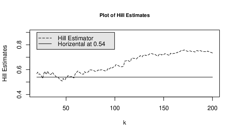
Since it is difficult to determine a range of such that (2.4) holds, we employ the Hill plot to help identify a range within which the Hill estimates are relatively stable. We first provide the plot of Hill’s estimates for for the sample fractions in the range from to . See Fig. 5. We observe that a turning point for the Hill estimator occurs around , and beyond this point the Hill plot shows an obvious upward trend, which indicates that the Hill estimates may be greatly influenced by the biases for large values of . In fact, when is in a range roughly from to , these Hill estimates are quite close.
We further compare the upper and lower limits for confidence intervals based on the normal approximation method and adjusted empirical likelihood method. See Fig. 6 for a plot in the range of between and . These lower confidence limits from two methods are close, but the upper limits of confidence intervals from the adjusted empirical likelihood method are obviously smaller than those from the normal approximation method for Hill’s estimator, and the lengths of the confidence intervals from the adjusted empirical method are uniformly shorter than those based on the normal approximation.


5 Proof of Theorem 3.1
We only provide a sketch of the proof. Note that we use to denote the true value of . Therefore, (2.3) is equivalent to
| (5.1) |
From equations (8) and (9) in the proof of Theorem 1 in Lu and Peng (2012), we have
| (5.2) |
| (5.3) |
The proof of (3.1), i.e., the proof of Theorem 1 in Lu and Peng (2002), requires only conditions (5.1) to (5.3). See Lu and Peng (2002) for details. Following the same lines in the proof, we only need to verify the following three similar conditions:
| (5.4) |
| (5.5) |
| (5.6) |
Since
equations (5.4) to (5.6) follows from (5.1) to (5.3), respectively. This completes the proof.
Acknowledgements: The authors would like to thank two anonymous referees for their constructive comments and suggestions that have led to improvements on the paper.
References
- [1] Chen, J., Variyath, A. M. and Abraham, B. (2008). Adjusted empirical likelihood and its properties. J. Comput. Graph. Statist. 17, 426-443.
- [2] Danielsson, J. and DeVries, C. (1997). Tail index and quantile estimation with very high frequency data. Journal of Empirical Finance 4, 241-257.
- [3] Danielsson, J., Hartmann, P., and De Vries, C. (1998). The cost of conservatism. Risk 11(1), 101-103.
- [4] De Haan, L. and Peng, L. (1998). Comparison of tail index estimators. Statistica Neerlandica 52, 60-70.
- [5] Drees, H. (1995). Refined Pickands estimators of the extreme value index. Ann. Statist. 23, 2059-2080.
- [6] Embrechts, P., Resnick, S., and Samorodnitsky, G. (1998). Living on the Edge. Risk 11(1), 96-100.
- [7] Embrechts, P., Resnick, S., and Samorodnitsky, G. (1999). Extreme value theory as a risk management tool. North American Actuarial Journal 3, 30-41.
- [8] Hall, P. (1982). On some simple estimators of an exponent of regular variation. J. Roy. Statist. Soc. Ser. B. 44, 37-42.
- [9] Hall, P. and Weissman, I. (1997). On the estimation of extreme tail probabilities. Ann. Statist. 25, 1311-1326.
- [10] Hill, B.M. (1975). A simple general approach to inference about the tail of a distribution. Ann. Statist. 3, 1163-1174.
- [11] Liu, Y. and Chen, J. (2010). Adjusted empirical likelihood with high-order precision. Ann. Statist. 3, 1341-1362.
- [12] Lu, J. and Peng L. (2002). Likelihood based confidence intervals for the tail index. Extremes 5, 337-352.
- [13] McNeil, A.J. (1997). Estimating the tails of loss severity distributions using extreme value theory. ASTIN Bulletin 27, 117-137.
- [14] Owen, A.B. (1988). Empirical likelihood ratio confidence intervals for a single functional. Biometrika 75, 237-249.
- [15] Owen, A.B. (1990). Empirical likelihood ratio confidence regions. Ann. Statist. 18, 90-120.
- [16] Peng, L. and Qi, Y. (2017). Inference for Heavy-Tailed Data: Applications in Insurance and Finance. Aacdemic Press.
- [17] Pickands III, J. (1975). Statistical inference using extreme order statistics. Ann. Statist. 3, 119-131.
- [18] Resnick, S. (1996). Discussion of the danish data on large fire insurance losses. Technical Report, www.casact.org/library/astin/vol27no1/139.pdf.
- [19] Tsao, M. (2004). A new method of calibration for the empirical loglikelihood ratio. Statist. Probab. Lett. 68, 305-314.
- [20] Weissman, I. (1978). Estimation of parameters and large quantiles based on the k largest observations. J. Amer. Statist. Assoc. 73, 812-815.