The $\boldsymbol{\chi_{cJ}}$ decay to $\boldsymbol{\phi K^{*}\bar{K},\phi h_{1}(1380)}$ testing the nature of axial vector meson resonances

The BESIII collaboration measured the $\chi_{cJ}\to\phi K^{*}(892)\bar{K}$ decay and found a clean signal around 1412 MeV and width 84 MeV that was associated to the $h_{1}(1380)$ production BES. As usual in experimental analysis, a Breit-Wigner shaped resonance was added incoherently to a background in the analysis and a fair reproduction of the data was found, except in the region 1550-1600 MeV where the data fall below the fitted results, showing a pronounced dip. In the present note we provide an explanation for this dip which is directly tied to the microscopic production process and the nature of the $h_{1}(1380)$ as a dynamically generated resonance.

The low lying axial vector meson resonances are fairly well described in a molecular picture from the vector-pseudoscalar interactions in $s$-wave using the interaction provided by chiral Lagrangians 9:Birse and a proper unitary procedure in vector-pseudoscalar coupled channels 5:Lutz; 6:Roca; 7:GengLS. It is then clear that within this picture the $\chi_{cJ}\to\phi h_{1}(1380)$ must proceed via the production $\chi_{cJ}\to\phi VP$ (with $V$ and $P$ denoting vector and pseudoscalar mesons, respectively), and a posterior interaction of $VP$ that will generate the resonance.

The first step in our analysis is to provide a picture for $\chi_{cJ}\to VVP$, where one of the vectors in particular will be the $\phi$. Since we are interested only in the shape of the final $K^{*}\bar{K}$ mass distribution, we can ignore the strength of this vertex, but we must relate the different possible trios with two vectors and one pseudoscalar. For this we are guided by theory and experiment. From the theoretical point of view we assume that $\chi_{cJ}$ is a SU(3) singlet since $\chi_{cJ}$, made of $c\bar{c}$, does not contain light quarks. Then we have a primary structure which is the trace $\langle VVP\rangle$ of the vector and pseudoscalar SU(3) matrices

where in $P$ we have considered to the $\eta$-$\eta^{\prime}$ mixing of Ref. 49:Bramon.

In the study of the $\chi_{c1}\to\eta\pi^{+}\pi^{-}$ reaction besKornicer, it was shown that the structure $\langle PPP\rangle$ for the vertex was favored by the experiment and the other possible structures $\langle PP\rangle\langle P\rangle$ and $\langle P\rangle^{3}$ were clearly rejected by experiment 46:Liang:chic1; 48:Vinicius:etac. In analogy to this, and prior to that work, it was found in Refs. 44:UGMOller; 45:Roca that in the $J/\psi\to\phi\pi^{+}\pi^{-},\omega\pi^{+}\pi^{-}$ reactions the most important structure was again $\langle VPP\rangle$, with a small component of $\langle V\rangle\langle PP\rangle$. This structure was again used in Ref. LiangSakai to study the $J/\psi\to\eta^{\prime}h_{1},\eta h_{1},\pi^{0}b_{1}$ reactions in connection with the BESIII experiment etaprime, where a fair agreement with experimental results was obtained using the same interaction as in Refs. 44:UGMOller; 45:Roca. In analogy to this, we propose now the structure

which should be dominant, where $\mathcal{C}$ is an arbitrary constant. A possible mixture of $\langle VV\rangle\langle P\rangle$ could change a bit the production rates, but we are only interested in the shape of the $K^{*}\bar{K}$ mass distribution which is not affected by this small admixture.

Equation (3), using the $P$ and $V$ matrices of Eqs. (2) and (1), gives the structure

which, ignoring the order and singling out the $\phi$ field, gives

Given the large mass of $\eta^{\prime}$, we neglect it in our study, as was also done in Ref. 6:Roca.

The structure with kaons that we have in Eq. (5) corresponds to the $\bar{K}^{*}K$ combination of isospin $I=0$ and $C$-parity $C=-$, with our convention ($K^{-}=-|1/2,-1/2\rangle,K^{*-}=-|1/2,-1/2\rangle,CK^{*+}=-K^{*-}$),

This convention is the same one used in Ref. 6:Roca and we can then take the coupling of the $h_{1}(1380)$ to the different channels from Ref. 6:Roca. The $\eta\phi$ term has also $I=0,C=-$, as it should be to match, together with the other $\phi$, the $\chi_{cJ}$ states.

Next we must look at the spin-parity structure of the vertices for the different $\chi_{cJ}$ states. When doing this we must take into account the order in which the fields appear in Eq. (4):

1. 1)

   $\chi_{c0}\to\phi K^{*}\bar{K}$    [$\chi_{c0}:I^{G}(J^{PC})=0^{+}(0^{+\,+})$]
   Since in the final state we have $V(1^{-})\,V(1^{-})\,P(0^{-})$, we need a $p$-wave to conserve parity. This eliminates structures like $\vec{\epsilon}_{\phi}\cdot\vec{\epsilon}_{K^{*}}$ or $(\vec{\epsilon}\cdot\vec{p}_{K})(\vec{\epsilon}_{K^{*}}\cdot\vec{p}_{\phi})$. The structure must be of the type

   $$(\vec{\epsilon}_{\phi}\times\vec{\epsilon}_{K^{*}})\cdot\vec{p}_{i},$$

   (7)

   with $\vec{p}_{i}$ some of the final momenta. This is indeed the operator used in the $dd\to\eta^{4}{\rm He}$ reaction hanhart; Ikeno; liangXie, which has the same quantum numbers. With these structures, if one selects for instance the $K^{*+}\phi K^{-}$ final channel, as shown diagrammatically in Fig. 1(a), one will get some contribution to the decay in this channel, as observed experimentally. Yet, if we wish to produce the $h_{1}(1380)$ resonance, we will have to consider the diagram of Fig. 1(b) and sum coherently in the loop over the states of Eq. (4). For this we must take care about the order in which the states appear in Eq. (4). Take first the term with momentum $\vec{p}_{K}$ in Eq. (7). We will have the combination

   $$2(\vec{\epsilon}_{K^{*}}\times\vec{\epsilon}_{\phi})\cdot\vec{p}_{K}+2(\vec{\epsilon}_{\phi}\times\vec{\epsilon}_{K^{*}})\cdot\vec{p}_{K}-\frac{1}{\sqrt{3}}(\vec{\epsilon}_{\phi_{1}}\times\vec{\epsilon}_{\phi_{2}})\cdot\vec{p}_{\eta}-\frac{1}{\sqrt{3}}(\vec{\epsilon}_{\phi_{2}}\times\vec{\epsilon}_{\phi_{1}})\cdot\vec{p}_{\eta}=0.$$

   (8)

   Next we would take the momentum of the two vectors and by symmetry we will have again

   			$\displaystyle 2(\vec{\epsilon}_{K^{*}}\times\vec{\epsilon}_{\phi})\cdot\vec{p}_{\phi}+2(\vec{\epsilon}_{\phi}\times\vec{\epsilon}_{K^{*}})\cdot\vec{p}_{K^{*}}+2(\vec{\epsilon}_{K^{*}}\times\vec{\epsilon}_{\phi})\cdot\vec{p}_{K^{*}}+2(\vec{\epsilon}_{\phi}\times\vec{\epsilon}_{K^{*}})\cdot\vec{p}_{\phi}$		(9)
   		$\displaystyle-$	$\displaystyle\frac{1}{\sqrt{3}}\left[(\vec{\epsilon}_{\phi_{1}}\times\vec{\epsilon}_{\phi_{2}})\cdot\vec{p}_{\phi_{2}}+(\vec{\epsilon}_{\phi_{1}}\times\vec{\epsilon}_{\phi_{2}})\cdot\vec{p}_{\phi_{1}}+(\vec{\epsilon}_{\phi_{2}}\times\vec{\epsilon}_{\phi_{1}})\cdot\vec{p}_{\phi_{1}}+(\vec{\epsilon}_{\phi_{2}}\times\vec{\epsilon}_{\phi_{1}})\cdot\vec{p}_{\phi_{2}}\right]$
   		$\displaystyle=$	$\displaystyle 0.$

   And we see that in the coherent sum the terms cancel and there is no $h_{1}(1380)$ production. This is the first output of our approach, since the assumed nature of the $h_{1}(1380)$ has as a consequence that the $h_{1}(1380)$ is not produced in the $\chi_{c0}\to\phi K^{*}\bar{K}$ reaction. This is corroborated by the experimental findings of Ref. BES.

2. 2)

   $\chi_{c1}\to\phi K^{*}\bar{K}$    [$\chi_{c1}:I^{G}(J^{PC})=0^{+}(1^{+\,+})$]
   Once again we need a $p$-wave and hence a momentum of the final particles. The argumentation is easy in the rest frame of $K^{*}\bar{K}(\bar{K}^{*}K)$. We will have a structure of the type

   $$(\vec{\epsilon}_{\chi_{c1}}\cdot\vec{p}_{i})(\vec{\epsilon}_{\phi}\cdot\vec{\epsilon}_{K^{*}}),$$

   (10)

   with $p_{i}$ any of the final momenta, or any cyclical permutation of this form (the $\phi\phi\eta$ term can be equally considered with $\epsilon_{\phi}\to\epsilon_{\phi_{1}}$, $\epsilon_{K^{*}}\to\epsilon_{\phi_{2}}$, plus keeping the symmetry of 1,2 for the two identical $\phi$ mesons). Take now the channel $K^{*+}\phi K^{-}$ of Eq. (4). Considering the symmetry of the two vectors we will have the combinations for the tree level of Fig. 1(a),

   $${\mathcal{C}}(\vec{\epsilon}_{\chi_{c1}}\cdot\vec{p}_{K})\;(\vec{\epsilon}_{\phi}\cdot\vec{\epsilon}_{K^{*}}),$$

   (11)

   $${\mathcal{C^{\prime}}}\left[(\vec{\epsilon}_{\chi_{c1}}\cdot\vec{p}_{K^{*}})+(\vec{\epsilon}_{\chi_{c1}}\cdot\vec{p}_{\phi})\right]\,(\vec{\epsilon}_{\phi}\cdot\vec{\epsilon}_{K^{*}}).$$

   (12)

   The terms that go with $\vec{p}_{K}$ or $\vec{p}_{K^{*}}$ involve $p$-wave and in the loops of Fig. 1(b) they will vanish.

   Hence, in the coherent sum of Fig. 1(b) for the loop of $VP$ we will get

   $$(\vec{\epsilon}_{\phi}\cdot\vec{\epsilon}_{K^{*}})\,(\vec{\epsilon}_{\chi_{c1}}\cdot\vec{p}_{\phi}),$$

   (13)

   which will be multiplied by the $G$ function and the $h_{1}$ amplitude later. This term will then interfere with the $s$-wave term of the tree level which has the same structure. Other terms in the tree level, which involve $p$-wave in $\vec{p}_{K}$, would not interfere with the loop term and would go into a background.

   The argument can be extended to any of the cyclical combinations of Eq. (10) with the same results, factorizing the same term involving $\vec{p}_{\phi}$ in the tree level and the loop contribution. Since we have an arbitrary normalization at the end, the whole discussion can be done with just the structure of Eq. (13).

3. 3)

   $\chi_{c2}\to\phi K^{*}\bar{K}$    [$\chi_{c2}:I^{G}(J^{PC})=0^{+}(2^{+\,+})$]
   Given the symmetry between the two vectors and what was found in points 1) and 2), it is clear that we should now combine the $\phi$ and $K^{*}$ spin to $J=2$ to avoid the cancellations found in point 1) where $J=1$ ( $\vec{\epsilon}_{\phi}\times\vec{\epsilon}_{K^{*}}$ combination). The spin 2 of the $\chi_{c2}$ can be combined with the $\vec{p}_{\phi}$ to give another tensor of rank two to be contracted with the $J=2$ object constructed with the two vectors. We would have remaining terms in the tree level and the loops involving $\vec{p}_{\phi}$ that would produce the $h_{1}(1380)$ resonance and some interference between them. We do not elaborate further since the calculations in what follow are only done for $\chi_{c1}$ decay. Experimentally one finds that the signal of $h_{1}(1380)$ is clearly seen in the $\chi_{c1}$ and $\chi_{c2}$ decays BES.

Next we must consider that in the experiment the $K^{*}$ is seen as a $K\pi$ state. If we want to have $K^{+}K^{-}\pi^{0}$, as experimentally measured, we can have

or

In these processes the $K^{+}$ is in $p$-wave in the first case and the $K^{-}$ is in $p$-wave in the second case. There is no interference upon angle integrations between the two mechanisms and their contributions would be the same. Since we are concerned only about the shape of the distributions, we consider only the first mechanism that we depict in Fig. 1.

The amplitude corresponding to the mechanisms of Fig. 1 is given by

where $A$ is a constant that contains $\mathcal{C}$ of Eq. (5) and a factor from the $K^{*}\to K\pi$ coupling, and the factor $\vec{p}_{K}-\vec{p}_{\pi}$ must be taken in the $K^{*}$ rest frame. In addition, $h_{K^{*+}K^{-}}$ and $h_{\phi\eta}$ are the weights of these states in the $H$ combination of Eq. (5) and $h_{K^{*}\bar{K}}$ the weight of the whole $K^{*}\bar{K},\bar{K}^{*}K$ combination in Eq. (5),

The factor $2$ in front of $h_{\phi\eta}$ in Eq. (14) stems from the identity of $\phi\phi$ in the Hamiltonian. The coupling $g_{h_{1},K^{*}\bar{K}}$ stands for the coupling of $h_{1}$ to the combination of Eq. (6), which is the one reported in Ref. 6:Roca. Similarly, $g_{h_{1},\phi\eta}$ is also taken from Ref. 6:Roca. The factor $2$ in front of $g_{h_{1},K^{*}\bar{K}}$ in Eq. (14) is because of the normalization of this state in $H$ of Eq. (5) compared to the normalization of the $K^{*}\bar{K}$ wave function of Ref. 6:Roca given in Eq. (6). In addition, $g_{h_{1},K^{*+}K^{-}}=\frac{1}{2}g_{h_{1},K^{*}\bar{K}}$ of Ref. 6:Roca. The couplings of $h_{1}(1380)$ to $K^{*}\bar{K}$ and $\phi\eta$ from Ref. 6:Roca are

The $D_{h_{1}}$, $D_{K^{*}}$ propagators of Eq. (14) are given by

with the mass $m_{h_{1}}$ and width $\Gamma_{h_{1}}$ of $h_{1}(1380)$ in the PDG pdg2018, and $G_{i}$ are the $VP$ loop functions that we take from Ref. 6:Roca using dimensional regularization with the same subtraction constant. In $G_{K^{*}\bar{K}}$, the width of $K^{*}$ is taken into account by means of a convolution using the $K^{*}$ spectral function.

Summing over the $K^{*}$ and $h_{1}$ polarizations in Eq. (14), we find

where $T$ is given by

When we sum and average over polarizations in $|t|^{2}$, we find at the end

where in $B$ we concentrate the different constant factors, and the double differential mass distribution is given by 51:Pavao

where

We integrate the differential width of Eq. (22) over $M_{\rm inv}(K^{+}\pi^{0})$ and compare the $\frac{{\rm d}\Gamma}{{\rm d}M_{\rm inv}(K^{*+}K^{-})}$ distribution with experiment.

For the $\chi_{c2}\to\phi K^{+}\pi^{0}K^{-}$ we would get the same formulas up to a possible different constant $B$ and the different mass of the $\chi_{c2}$. We have seen that the shape of the $K^{+}K^{-}\pi^{0}$ mass distribution for the $\chi_{c2}$ decay is practically the same as for the $\chi_{c1}$ decay in the range that we are interested in. Actually this is also the case for the BESIII experiment BES. Finally, we do not evaluate the mass distribution for the $\chi_{c1}\to K_{S}^{0}K^{\pm}\pi^{\mp}$ decay, but based on the possible $K^{*}\bar{K}$, $\bar{K}^{*}K$ modes leading to this distribution we get a rate twice as large as for the $K^{+}K^{-}\pi^{0}$ decay, as clearly seen in the experiment, and the same shape as the one calculated. In view of these findings, we can compare the results that we obtain, up to an arbitrary normalization, with those of Ref. BES for the sum of all these modes, which is done to gain statistics.

In Fig. 2 we can see the contribution to $\frac{{\rm d}\Gamma}{{\rm d}M_{\rm inv}(K^{*+}K^{-})}$ from the first term of $T$ in Eq. (20) (tree level), the second term that contains the $h_{1}(1380)$ propagator (“Loop” in the figure) and the coherent sum.

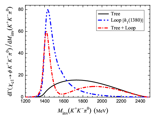
The interesting finding is that the tree level, which by itself could be considered a background and contributes basically according to phase space, interferes destructively with the $h_{1}(1380)$ signal and the resulting shape is quite different from the one of the $h_{1}(1380)$ itself, which has a much broader shape. It is interesting to see that our contribution of the $h_{1}(1380)$ alone has basically the same shape as the one of Ref. BES in Fig. 7 of that work. In addition, in Ref. BES a background, and the $\phi(1680)$ and $\phi(1850)$ contributions are added incoherently. The interference between the tree level mechanism and the $h_{1}(1380)$ contribution is then missed in that analysis. It is clear that our approach will show a dip in the region of 1550-1600 MeV of the $K^{+}K^{-}\pi^{0}$ invariant mass.

In order to compare the mass distribution $\frac{{\rm d}\Gamma}{{\rm d}M_{\rm inv}(K^{*+}K^{-})}$ of Ref. BES, we also add a background and the $\phi(1680)$ contribution, since we are not interested in the region where the $\phi(1850)$ can contribute. We modify minimally the input of Ref. BES, but some different normalization is needed in view of the interference that we have mentioned. Our signal for the $h_{1}(1380)$ of the peak is multiplied by 1.2 and the background by 1.3 while, we keep the same strength at the peak of the $\phi(1680)$ as in Ref. BES. The results are shown in Fig. 3.

There is also another small difference in the $\phi(1680)$ contribution since its decay into $K^{*}\bar{K}$ must proceed in $p$-wave and hence we have a contribution of the type

where $D$ is a constant, and

with $M_{\phi(1680)}$ and $\Gamma^{(0)}_{\phi(1680)}$ being the mass and width of $\phi(1680)$.

What we see in Fig. 3 is that our approach produces naturally a clear dip in the region of 1550-1600 MeV, while the fit of Ref. BES gives a distribution that is above the data in that region. It is clear that the experimental fit will give a larger strength in that region than our approach because they do not have the interference of the background with the resonance that we have shown in our approach. Certainly a different fit to the data could have been done putting a tree level and the signal of the $h_{1}(1380)$ and letting them interfere, however, in that fit, the strength of the tree level and its sign would be uncorrelated. In our approach the relative strength and sign are given once we assume that the $h_{1}(1380)$ is generated from the interaction between pseudoscalar and vector. This is why the dip which we predict for this distribution is tied to the nature of the $h_{1}(1380)$ as a dynamically generated resonance, and the fact that this feature is present in the experiment provides a great support for that picture of the $h_{1}(1380)$, and by analogy other axial vector meson resonances as dynamically generated from the vector-pseudoscalar interaction.

In summary, based on the picture that the $h_{1}(1380)$ is a dynamically generated resonance formed from the interaction of vector-pseudoscalar pairs, mostly $K^{*}\bar{K}-c.c.$ and $\phi\eta$, we have carried out a study of the $\chi_{cJ}\to\phi K^{*}\bar{K}\to\phi K^{+}\pi^{0}K^{-}$ reaction and related charge channels and have obtained a fair reproduction of the shape of the experimental data. Due to the fact that in this picture the $h_{1}(1380)$ is generated from the $s$-wave $VP$ interaction, we could justify why no $h_{1}(1380)$ signal was found in the $\chi_{c0}$ decay, while the signal appeared both in the $\chi_{c1}$ and $\chi_{c2}$ decays. Another remarkable feature of the study was that we could determine the relative strength between the tree level contribution to the process and the one that contains the $h_{1}(1380)$ production, and we found a destructive interference between the two processes that significantly distorts the $h_{1}(1380)$ signal with respect to the Breit-Wigner shape and produces a dip in the $K^{+}\pi^{0}K^{-}$ mass distribution around the region of 1550-1600 MeV. This dip is present in the experiment and not reproduced in a picture that sums incoherently the $h_{1}$ Breit-Wigner distribution with a smooth background, providing a strong support to the molecular picture of the $h_{1}(1380)$ resonance.