跳到论文正文
W Papers独立论文阅读器 arXiv:1904.08212 论文正文 计算阅读时间 · 0%
引用这篇论文根据当前论文元数据生成,正式投稿前建议核对。


License: arXiv.org perpetual non-exclusive license
arXiv:1904.08212v2 [math.PR] 13 Apr 2021

Upper tails via high moments and entropic stabilityThanks: This research is supported in part by the Israel Science Foundation grants 1147/14 (FM and WS), 1028/16 (FM), and 1145/18 (FM and WS), the ERC Starting Grant 633509 (FM) and 678520 (MH), and the Zuckerman Postdoctoral Fellowship Program (MH)

Matan Harel Address: Matan Harel, Department of Mathematics, Northeastern University, Boston, MA 02115, USA Email address: m.harel@northeastern.edu , Frank Mousset Address: Frank Mousset, School of Mathematical Sciences, Tel Aviv University, Tel Aviv 6997801, Israel Email address: moussetfrank@gmail.com and Wojciech Samotij Address: Wojciech Samotij, School of Mathematical Sciences, Tel Aviv University, Tel Aviv 6997801, Israel Email address: samotij@tauex.tau.ac.il
Date: August 11, 2026
Abstract.

Suppose that XX is a bounded-degree polynomial with nonnegative coefficients on the pp-biased discrete hypercube. Our main result gives sharp estimates on the logarithmic upper tail probability of XX whenever an associated extremal problem satisfies a certain entropic stability property. We apply this result to solve two long-standing open problems in probabilistic combinatorics: the upper tail problem for the number of arithmetic progressions of a fixed length in the pp-random subset of the integers and the upper tail problem for the number of cliques of a fixed size in the random graph Gn,pG_{n,p}. We also make significant progress on the upper tail problem for the number of copies of a fixed regular graph HH in Gn,pG_{n,p}. To accommodate readers who are interested in learning the basic method, we include a short, self-contained solution to the upper tail problem for the number of triangles in Gn,pG_{n,p} for all p=p⁡(n)p=p(n) satisfying n−1​log⁡n≪p≪1n^{-1}\log n\ll p\ll 1.

1. Introduction

Suppose that Y=(Y1,…,YN)Y=(Y_{1},\dotsc,Y_{N}) is a sequence of independent Bernoulli random variables with mean pp and that X=X⁡(Y)X=X(Y) is an NN-variate polynomial with nonnegative real coefficients. Perhaps the simplest question that can be asked about the typical behaviour of XX is whether it satisfies a law of large numbers, i.e., whether X→𝔼⁡[X]X\to\e[X] in probability as N→∞N\to\infty. Once this is established, it is natural to ask for quantitative estimates of the probability of the event that XX differs from its mean by a significant amount. In the special case where Y↦X⁡(Y)Y\mapsto X(Y) is a linear function, this problem is addressed by the classical theory of large deviations, see [14, 28]. This theory shows that, under mild conditions on the coefficients of the linear function XX and the assumptions p→0p\to 0 and N​p→∞Np\to\infty,

ℙ⁡(|X−𝔼⁡[X]|⩾δ​𝔼⁡[X])=e−(I⁡(δ)+o⁡(1))​Np\mathbb{P}\big(|X-\e[X]|\geqslant\delta\e[X]\big)=e^{-(I(\delta)+o(1))Np}

for an explicitly computable function I:(0,∞)→(0,∞]I\colon(0,\infty)\to(0,\infty]. However, there are many natural situations where one would like to consider nonlinear polynomials X⁡(Y)X(Y), as in the following two examples. We use the notation ⟦N⟧={1,…,N}\llbracket{N}\rrbracket=\{1,\dotsc,N\}.

1.1Arithmetic progressions in random sets of integers.

A kk-term arithmetic progression is a sequence of kk integers of the form (a,a+b,a+2​b,…,a+(k−1)​b)\big(a,a+b,a+2b,\dotsc,a+(k-1)b\big), where b>0b>0. We write ⟦N⟧p\llbracket{N}\rrbracket_{p} for the random subset of ⟦N⟧\llbracket{N}\rrbracket obtained by including every element of ⟦N⟧\llbracket{N}\rrbracket independently with probability pp. Let XN,pk-APX_{N,p}^{\text{$k$-AP}} denote the number of kk-term arithmetic progressions in ⟦N⟧p\llbracket{N}\rrbracket_{p}. Then XN,pk-APX_{N,p}^{\text{$k$-AP}} can be considered as a polynomial with nonnegative coefficients and degree kk in the independent Ber⁡(p)\mathrm{Ber}(p) random variables Y1,…,YNY_{1},\dotsc,Y_{N}, where YiY_{i} is the indicator variable of the event that i∈⟦N⟧pi\in\llbracket{N}\rrbracket_{p}; explicitly,

XN,pk-AP=∑b>0∑a⩾1a+(k−1)​b⩽N∏i=0k−1Ya+i​b.X_{N,p}^{\text{$k$-AP}}=\sum_{b>0}\sum_{\begin{subarray}{c}a\geqslant 1\\ a+(k-1)b\leqslant N\end{subarray}}\prod_{i=0}^{k-1}Y_{a+ib}.

We remark that, unlike [10] and several other works, we count only genuine arithmetic progressions (i.e., we do not consider degenerate progressions of the form (a,…,a)(a,\dotsc,a)) and we count every progression only once (as opposed to counting (a1,a2,…,ak)(a_{1},a_{2},\dotsc,a_{k}) and (ak,ak−1,…,a1)(a_{k},a_{k-1},\dotsc,a_{1}) as two different progressions).

1.2Subgraph counts in random graphs.

Fix a nonempty graph HH and let Xn,pHX^{H}_{n,p} be the number of copies of HH in the random graph Gn,pG_{n,p}, that is, the number of subgraphs of Gn,pG_{n,p} isomorphic to HH. Then Xn,pHX_{n,p}^{H} can be written as a polynomial with nonnegative coefficients and degree eHe_{H} in the N=(n2)N=\binom{n}{2} indicator random variables of the possible edges of Gn,pG_{n,p}. More precisely, fix an arbitrary bijection σn:(⟦n⟧2)→⟦N⟧\sigma_{n}\colon\binom{\llbracket{n}\rrbracket}{2}\to\llbracket{N}\rrbracket (the precise choice is irrelevant) and, for every i∈⟦N⟧i\in\llbracket{N}\rrbracket, let YiY_{i} be the indicator variable of the event that σn−1​(i)\sigma_{n}^{-1}(i) is an edge in Gn,pG_{n,p}. Then Y1,…,YNY_{1},\dotsc,Y_{N} are independent Ber⁡(p)\mathrm{Ber}(p) random variables and

Xn,pH=∑H′⊆KnH′≅H∏e∈E⁡(H′)Yσn​(e),X_{n,p}^{H}=\sum_{\begin{subarray}{c}H^{\prime}\subseteq K_{n}\\ H^{\prime}\cong H\end{subarray}}\prod_{e\in E(H^{\prime})}Y_{\sigma_{n}(e)},

where KnK_{n} denotes the complete graph on the vertex set ⟦n⟧\llbracket{n}\rrbracket and ≅{\cong} denotes the isomorphism relation on graphs.

In this paper, we will always assume that δ\delta is fixed and p→0p\to 0 as N→∞N\to\infty.

The large deviation problem for the variables described above is significantly more involved than the linear case; in particular, the lower and upper tail probabilities—that is, ℙ⁡(X⩽(1−δ)​𝔼⁡[X])\mathbb{P}\big(X\leqslant(1-\delta)\e[X]\big) and ℙ⁡(X⩾(1+δ)​𝔼⁡[X])\mathbb{P}\big(X\geqslant(1+\delta)\e[X]\big), respectively—exhibit dramatically different behaviours. On the one hand, using a combination of Harris’s inequality [41] and Janson’s inequality [43], one can show that X=XN,pk-APX=X_{N,p}^{\text{$k$-AP}} satisfies

(1) e−C1​(δ)​min⁡{𝔼⁡[X],Np}⩽ℙ⁡(X⩽(1−δ)​𝔼⁡[X])⩽e−C2​(δ)​min⁡{𝔼⁡[X],Np}e^{-C_{1}(\delta)\min{\{\e[X],Np\}}}\leqslant\mathbb{P}\big(X\leqslant(1-\delta)\e[X]\big)\leqslant e^{-C_{2}(\delta)\min{\{\e[X],Np\}}}

for some positive C1​(δ)C_{1}(\delta) and C2​(δ)C_{2}(\delta); similar bounds are available for X=Xn,pHX=X_{n,p}^{H}.11 1 For more precise results, we refer the interested reader to [48, 54, 58, 71]. On the other hand, there are no comparably simple tools that allow one to easily obtain similar estimates on the logarithm of the upper tail probability. The standard concentration inequalities due to Azuma–Hoeffding [42], Talagrand [64], or Kim–Vu [52, 68] yield bounds that are far from tight in Examples 1.1 and 1.2. For a survey discussing these and other classical approaches to the ‘infamous upper tail’ problem, see [45].

Unlike the lower tail, the upper tail is susceptible to the influence of small structures whose appearance increases the value XX atypically, a phenomenon that we refer to as localisation. For example, in the case of X=XN,pk-APX=X_{N,p}^{\text{$k$-AP}} where k⩾3k\geqslant 3, a typical subset of size m=o⁡(N)m=o(N) contains Θ⁡(N2​(m/N)k)=o⁡(m2)\Theta\big(N^{2}(m/N)^{k}\big)=o(m^{2}) kk-term arithmetic progressions, whereas some very rare subsets (notably an interval of length mm) can contain as many as Θ⁡(m2)\Theta(m^{2}) such progressions. The event that ⟦N⟧p\llbracket{N}\rrbracket_{p} contains an interval of length Θ⁡(𝔼⁡[X])\Theta(\sqrt{\e[X]}) thus provides a lower bound on the upper tail probability. More precisely, ℙ⁡(X⩾(1+δ)​𝔼⁡[X])⩾exp⁡(−O⁡(𝔼⁡[X]​log⁡(1/p)))\mathbb{P}\big(X\geqslant(1+\delta)\e[X]\big)\geqslant\exp\big(-O(\sqrt{\e[X]}\log(1/p))\big), which is significantly larger than the lower tail probability (1) for most pp. In order to properly analyse the upper tail event, one must account for these local effects, which frequently requires understanding the peculiar combinatorial nature of the random variable XX.

The last decade has seen the development of an increasingly powerful theory of ‘nonlinear large deviations’, which began with the work of Chatterjee–Dembo [18] and was further developed by Eldan [30], Cook–Dembo [24], Augeri [2, 3], and Cook–Dembo–Pham [25]. Whenever a general function ff of i.i.d. random variables satisfies certain complexity and regularity conditions, these results can be used to express the upper tail probability ℙ⁡(f⩾(1+δ)​𝔼⁡[f])\mathbb{P}\big(f\geqslant(1+\delta)\e[f]\big) in terms of an associated variational problem. In the case where ff is a polynomial with nonnegative coefficients on the hypercube, this variational problem is able to capture the presence of localisation, if it occurs. In the two examples mentioned above, nonlinear large deviation theory gives tight control of the upper tail probabilities whenever p⩾N−αp\geqslant N^{-\alpha} for some constant α>0\alpha>0. However, the best-known constant α\alpha is not optimal in both examples.

Our main contribution is a general method for proving sharp bounds on the upper tail probability of the polynomial X=X⁡(Y)X=X(Y) in the presence of localisation. In many cases where localisation occurs, our approach can also give a coarse description of the tail event. At the heart of our method lies an adaptation of the classical moment argument of Janson, Oleszkiewicz, and Ruciński [44], which we use to formalise the intuition that the upper tail event is dominated by the appearance of near-minimisers of the combinatorial optimisation problem

(2) ΦX​(δ)=min⁡{|I|​log⁡(1/p):I⊆⟦N⟧​ and ​𝔼⁡[X∣Yi=1​ for all i∈I]⩾(1+δ)​𝔼⁡[X]}.\Phi_{X}(\delta)=\min{\big\{|I|\log(1/p):I\subseteq\llbracket{N}\rrbracket\text{ and }\e[X\mid Y_{i}=1\text{ for all $i\in I$}]\geqslant(1+\delta)\e[X]\big\}}.

Roughly speaking, we say that I⊆⟦N⟧I\subseteq\llbracket{N}\rrbracket is a core if it is a feasible set for the above optimisation problem, its size is O​(ΦX​(δ))O\big(\Phi_{X}(\delta)\big), and it satisfies a certain natural rigidity condition that arises from requiring every element in the set to contribute a sizeable amount to the expectation. The constraints used to define a core are loosely analogous to the complexity conditions used in nonlinear large deviation theory; we will give a more precise definition of a core and discuss its relations to earlier work in more detail in Section 3.

We show that the upper tail probability is approximately equal to the probability of the appearance of a core. In particular, when the number of cores of size mm is (1/p)o⁡(m)(1/p)^{o(m)}, a property we term entropic stability, then a union bound implies that −log⁡ℙ⁡(X⩾(1+δ)​𝔼⁡[X])-\log\mathbb{P}\big(X\geqslant(1+\delta)\Ex[X]\big) is well approximated by ΦX​(δ)\Phi_{X}(\delta). We will verify that the random variables XN,pk-APX_{N,p}^{\text{$k$-AP}} and Xn,pHX_{n,p}^{H} (for a large class of graphs HH) satisfy the entropic stability condition under optimal, or nearly optimal, assumptions on pp.22 2 We use the phrase entropic stability in a similar sense to the notion of stability in extremal combinatorics. More precisely, we are considering situations where the probability that ∏i∈IYi=1\prod_{i\in I}Y_{i}=1 for some minimiser II of (2) is asymptotically equal to the probability of appearance of one such minimiser—in other words, the energy of such configurations (given by the number of elements involved) dominates over the entropy (that is, the number of such configurations). Then entropic stability means that the entropy term remains negligible even as we move away from true minimisers of (2) to sets that are merely close to being minimisers (the cores).

One important caveat that we have ignored so far is that the upper tail exhibits localisation only when the expectation of XX tends to infinity sufficiently quickly. In fact, if 𝔼⁡[X]\e[X] is of constant order, then, under relatively mild conditions, XX converges in distribution to a Poisson random variable and no localisation occurs. We show that, for the two examples discussed above, the upper tail continues to have Poisson behaviour even when 𝔼⁡[X]\e[X] goes to infinity sufficiently slowly. In the cases of kk-term arithmetic progressions in ⟦N⟧p\llbracket{N}\rrbracket_{p} and cliques in Gn,pG_{n,p}, our results for the Poisson and localised regimes cover almost the whole range of densities p→0p\to 0 with 𝔼⁡[X]→∞\e[X]\to\infty, leaving the upper tail probability undetermined only at densities for which it is believed that the two behaviours coexist.

1.1. Arithmetic progressions in random sets of integers

Let X=XN,pk-APX=X_{N,p}^{\text{$k$-AP}} denote the number of kk-term arithmetic progressions in ⟦N⟧p\llbracket{N}\rrbracket_{p}. It is not hard to see that 𝔼⁡[X]=Θ⁡(N2​pk)\e[X]=\Theta(N^{2}p^{k}). Whenever this expectation vanishes, the upper tail event is commensurate with the probability of X⩾1X\geqslant 1, which can be controlled using Markov’s inequality. More generally, if 𝔼⁡[X]\e[X] is bounded, then it follows from standard techniques that XX is asymptotically Poisson [7]; in this case, the large deviations of XX are those of a Poisson random variable with mean 𝔼⁡[X]\e[X]. For the remainder of this section, we shall thus assume that 𝔼⁡[X]→∞\e[X]\to\infty, i.e., that pk/2≫N−1p^{k/2}\gg N^{-1}.

Improving an earlier estimate due to Janson and Ruciński [47], Warnke [69] proved that under fairly general assumptions (in particular, for constant δ>0\delta>0 and all pp bounded away from 11),

(3) −log⁡ℙ⁡(X⩾(1+δ)​𝔼​[X])=Θ⁡(min⁡{((1+δ)​log⁡(1+δ)−δ)​𝔼​[X],δ​𝔼⁡[X]​log⁡(1/p)}),-\log\mathbb{P}(X\geqslant(1+\delta)\e[X])=\Theta\left(\min\left\{\big((1+\delta)\log(1+\delta)-\delta\big)\e[X],\sqrt{\delta\e[X]}\log(1/p)\right\}\right),

where the constants implicit in the Θ\Theta-notation are independent of δ\delta. Note that the two terms of the minimum correspond to the dominance of the Poisson and the localised regimes, respectively.

Since then, it has been an open problem to determine the missing constant factor in (3). Using the above-mentioned framework of Eldan [30], Bhattacharya, Ganguly, Shao, and Zhao [10] were able to do so in the range N−112​(k−1)​(log⁡N)O⁡(1)≪pk/2≪1N^{-\frac{1}{12(k-1)}}(\log N)^{O(1)}\ll p^{k/2}\ll 1. This was subsequently improved by Briët–Gopi [15] to the slightly wider range N−112​⌈(k−1)/2⌉​(log⁡N)O⁡(1)≪pk/2≪1N^{-\frac{1}{12\lceil(k-1)/2\rceil}}(\log N)^{O(1)}\ll p^{k/2}\ll 1, also using Eldan’s result. The two theorems below improve significantly on these results and determine the precise rate of the upper tail for all N−1≪pk/2≪1N^{-1}\ll p^{k/2}\ll 1, excepting the case pk/2=Θ⁡(N−1​log⁡N)p^{k/2}=\Theta(N^{-1}\log N). The first result concerns the range where the minimum in (3) is δ​𝔼⁡[X]​log⁡(1/p)\sqrt{\delta\e[X]}\log(1/p).

1.3.

Let k⩾3k\geqslant 3 be an integer and let X=XN,pk-APX=X_{N,p}^{\text{$k$-AP}} denote the number of kk-term arithmetic progressions in ⟦N⟧p\llbracket{N}\rrbracket_{p}. Then, for every fixed positive constant δ\delta and all p=p⁡(N)p=p(N) satisfying N−1​log⁡N≪pk/2≪1N^{-1}\log N\ll p^{k/2}\ll 1,

limN→∞−log⁡ℙ⁡(X⩾(1+δ)​𝔼⁡[X])N​pk/2​log⁡(1/p)=δ.\lim_{N\to\infty}\frac{-\log\mathbb{P}\big(X\geqslant(1+\delta)\e[X]\big)}{Np^{k/2}\log(1/p)}=\sqrt{\delta}.

Observe that Theorem 1.3 shows that the upper tail probability is well approximated by the probability of appearance of an interval (or, more generally, an arithmetic progression) of length δ​N2​pk\sqrt{\delta N^{2}p^{k}} in ⟦N⟧p\llbracket{N}\rrbracket_{p}. Since each such interval contains approximately δ​𝔼⁡[X]\delta\Ex[X] arithmetic progressions of length kk, it is not hard to see that conditioning ⟦N⟧p\llbracket{N}\rrbracket_{p} on the appearance of such a set will cause the upper tail event to occur with sizable probability. Conversely, our methods may be used to prove that the upper tail event is dominated by the appearance of some set of size (1+o⁡(1))​δ​N2​pk(1+o(1))\sqrt{\delta N^{2}p^{k}} that contains nearly δ​𝔼⁡[X]\delta\Ex[X] arithmetic progressions of length kk. It seems natural to guess that each such set is, in some sense, close to an arithmetic progression. However, this is not the case, as was shown by Green–Sisask [37]. We currently do not know a structural characterisation of the sets described above, which prevents us from proving a qualitative description of the upper tail event. For further discussion, we refer to Section 10.

The second result treats the complementary range N−1≪pk/2≪N−1​log⁡NN^{-1}\ll p^{k/2}\ll N^{-1}\log N, where the upper tail has Poisson behaviour.

1.4.

Let k⩾3k\geqslant 3 be an integer and let X=XN,pk-APX=X_{N,p}^{\text{$k$-AP}} denote the number of kk-term arithmetic progressions in ⟦N⟧p\llbracket{N}\rrbracket_{p}. Then, for every fixed positive constant δ\delta and all p=p⁡(N)p=p(N) satisfying N−1≪pk/2≪N−1​log⁡NN^{-1}\ll p^{k/2}\ll N^{-1}\log N,

limN→∞−log⁡ℙ⁡(X⩾(1+δ)​𝔼⁡[X])𝔼⁡[X]=(1+δ)​log⁡(1+δ)−δ.\lim_{N\to\infty}\frac{-\log\mathbb{P}\big(X\geqslant(1+\delta)\e[X]\big)}{\e[X]}=(1+\delta)\log(1+\delta)-\delta.

1.2. Subgraph counts in random graphs

Let X=XN,pHX=X_{N,p}^{H} be the number of copies of a  fixed graph HH in Gn,pG_{n,p}. Note that 𝔼⁡[X]=Θ⁡(nvH​peH)\e[X]=\Theta(n^{v_{H}}p^{e_{H}}). Since controlling the distribution of XX for completely general graphs involves many technical difficulties (see for example [12, 66]), we will restrict our attention to connected, Δ\Delta-regular graphs HH. If the expected value of XX is bounded, then XX converges to a Poisson random variable, as was shown independently by Bollobás [11] and by Karoński–Ruciński [49]. In view of this, for the remainder of this section, we shall assume that 𝔼⁡[X]→∞\e[X]\to\infty, i.e., that pΔ/2≫n−1p^{\Delta/2}\gg n^{-1}. As mentioned before, we will also assume that p→0p\to 0; the case where p∈(0,1)p\in(0,1) is fixed, which is fundamentally different, was addressed in [21, 56, 59].

The problem of controlling the upper tail of XX has a long history. A sequence of papers [46, 53, 68], culminating in the work of Janson, Oleszkiewicz, and Ruciński [44], resulted in upper and lower bounds on the logarithmic upper tail probability that differed by a multiplicative factor of log⁡(1/p)\log(1/p). In the case where HH is a clique, Chatterjee [16] and DeMarco–Kahn [26] independently added the missing logarithmic factor to the upper bound, thus establishing the order of magnitude of the logarithmic upper tail probability. The theory of nonlinear large deviations (discussed above) provides a variational description of the dependence of the upper tail probability ℙ⁡(X⩾(1+δ)​𝔼⁡[X])\mathbb{P}(X\geqslant(1+\delta)\e[X]) on δ\delta for a certain range of p→0p\to 0, as established in [3, 18, 24, 25, 30]; the strongest of these results require p≫n−1/(Δ+1)p\gg n^{-1/(\Delta+1)} for general graphs of maximal degree Δ\Delta [24, 25], and pΔ/2≫n−1/2p^{\Delta/2}\gg n^{-1/2} for the case where HH is a cycle [3, 24] (disregarding polylogarithmic factors). The associated variational problem was solved by Lubetzky–Zhao [57] when HH is a clique and by Bhattacharya, Ganguly, Lubetzky, and Zhao [9] for general HH. For a more detailed overview of these techniques, we refer the reader to the book of Chatterjee [17].

The solution to the variational problem is expressed in terms of the independence polynomial of a graph. For any HH, define PH​(x)=∑kik​(H)​xkP_{H}(x)=\sum_{k}i_{k}(H)x^{k}, where ik​(H)i_{k}(H) is the number of independent sets of HH of size kk, and let θ=θ⁡(δ)\theta=\theta(\delta) be the unique positive solution to PH​(θ)=1+δP_{H}(\theta)=1+\delta.33 3 We note that i0​(H)=1i_{0}(H)=1 for every graph HH, so that, for example, PKr​(x)=1+r​xP_{K_{r}}(x)=1+rx. There are two constructions that yield lower bounds for the upper tail probability (see Figure 1). In both cases, one plants a ‘small’ subgraph whose presence ensures that Gn,pG_{n,p} contains (1+δ)​𝔼⁡[X](1+\delta)\e[X] copies of HH with good probability. The first of these subgraphs is a clique on δ1/vH​n​pΔ/2\delta^{1/v_{H}}np^{\Delta/2} vertices (as in the left side of the figure), which contains the extra δ​𝔼⁡[X]\delta\e[X] copies of HH required by the upper tail event (up to lower-order corrections). The second subgraph (which is often called a ‘hub’) is a complete bipartite graph with parts of size θ​n​pΔ\theta np^{\Delta} and n−θ​n​pΔn-\theta np^{\Delta}, respectively (as in the right side of the figure); since we are implicitly assuming that θ​n​pΔ\theta np^{\Delta} is an integer, rounding errors play a significant role here unless n​pΔ≫1np^{\Delta}\gg 1. A short calculation shows that the expected number of copies of HH which intersect this graph is approximately δ​𝔼⁡[X]\delta\e[X] and thus the actual number of such copies is almost δ​𝔼⁡[X]\delta\e[X] with good probability. In both cases, the complement of the planted subgraph typically contains approximately 𝔼⁡[X]\e[X] copies of HH. Formalising this argument, one obtains the two lower bounds

ℙ⁡(X⩾(1+δ)​𝔼⁡[X])⩾p(δ2/vH+o⁡(1))​n2​pΔandℙ⁡(X⩾(1+δ)​𝔼⁡[X])⩾p(θ+o⁡(1))​n2​pΔ,\mathbb{P}\big(X\geqslant(1+\delta)\e[X]\big)\geqslant p^{(\delta^{2/v_{H}}+o(1))n^{2}p^{\Delta}}\quad\text{and}\quad\mathbb{P}\big(X\geqslant(1+\delta)\e[X]\big)\geqslant p^{(\theta+o(1))n^{2}p^{\Delta}},

which correspond to planting the clique and the complete bipartite graph, respectively. (Recall that the latter bound is valid only when n​pΔ≫1np^{\Delta}\gg 1.)

Our main result is that, when HH is not bipartite, one of the above bounds is tight in nearly the whole range of densities. When HH is bipartite, we prove tight bounds on the logarithmic upper tail probability only when pΔ/2⩾n−1/2−o(1)p^{\Delta/2}\geqslant n^{-1/2-o(1)}.

δ1/vH​n​pΔ/2\delta^{1/v_{H}}np^{\Delta/2}nnθ​n​pΔ\theta np^{\Delta}n−θ​n​pΔn-\theta np^{\Delta}
Figure 1. The two constructions giving lower bounds for the upper tail probability of X=Xn,pHX=X_{n,p}^{H}.
1.5.

Let Δ⩾2\Delta\geqslant 2 be an integer, let HH be a connected, nonbipartite, Δ\Delta-regular graph, and let X=XN,pHX=X_{N,p}^{H} denote the number of copies of HH in Gn,pG_{n,p}. Then for every fixed positive constant δ\delta and all p=p⁡(n)p=p(n) satisfying n−1​(log⁡n)Δ​vH2≪pΔ/2≪1n^{-1}(\log n)^{\Delta v_{H}^{2}}\ll p^{\Delta/2}\ll 1,

limn→∞−log⁡ℙ⁡(X⩾(1+δ)​𝔼⁡[X])n2​pΔ​log⁡(1/p)={δ2/vH/2if n​pΔ→0,min⁡{δ2/vH/2,θ}if n​pΔ→∞,\lim_{n\to\infty}\frac{-\log\mathbb{P}\big(X\geqslant(1+\delta)\e[X]\big)}{n^{2}p^{\Delta}\log(1/p)}=\begin{cases}\delta^{2/v_{H}}/2&\text{if $np^{\Delta}\to 0$,}\\ \min{\{\delta^{2/v_{H}}/2,\theta\}}&\text{if $np^{\Delta}\to\infty$},\end{cases}

where θ\theta is the unique positive solution to PH​(θ)=1+δP_{H}(\theta)=1+\delta. Additionally, if pΔ/2⩾n−1/2−o(1)p^{\Delta/2}\geqslant n^{-1/2-o(1)}, then the assumption that HH is nonbipartite is not necessary.

We note that the theorem leaves open the case where n​pΔ→c∈(0,∞)np^{\Delta}\to c\in(0,\infty). In this regime, the explicit dependence of the upper tail probability on δ\delta involves various integrality conditions and is therefore quite complicated. In the next subsection, we explicitly treat this regime when HH is a clique. The assumption of nonbipartiteness is not phenomenological, but only technical. The aforementioned entropic stability condition, which plays a crucial role in our proof, ceases to hold when HH is bipartite as soon as pΔ/2⩽n−1/2−Θ(1)p^{\Delta/2}\leqslant n^{-1/2-\Theta(1)}, see Section 10.

Our next result concerns the Poisson regime of the upper tail.

1.6.

Let Δ⩾2\Delta\geqslant 2 be an integer, let HH be a connected, Δ\Delta-regular graph, and let X=Xn,pHX=X_{n,p}^{H} denote the number of copies of HH in Gn,pG_{n,p}. Then, for every fixed positive constant δ\delta and all p=p⁡(n)p=p(n) satisfying n−1≪pΔ/2≪n−1​(log⁡n)1vH−2n^{-1}\ll p^{\Delta/2}\ll n^{-1}(\log n)^{\frac{1}{v_{H}-2}},

limn→∞−log⁡ℙ⁡(X⩾(1+δ)​𝔼⁡[X])𝔼⁡[X]=(1+δ)​log⁡(1+δ)−δ.\lim_{n\to\infty}\frac{-\log\mathbb{P}\big(X\geqslant(1+\delta)\e[X]\big)}{\e[X]}=(1+\delta)\log(1+\delta)-\delta.

In the case where HH is a clique, DeMarco and Kahn [26] proved that the logarithmic upper tail probability is of order 𝔼⁡[X]\e[X] throughout the regime covered by Theorem 1.6. For other Δ\Delta-regular graphs HH, the analogous fact was known only in the range n−1≪pΔ/2≪n−1​(log⁡n)cHn^{-1}\ll p^{\Delta/2}\ll n^{-1}(\log n)^{c_{H}}, for some positive constant cH<1/(vH−2)c_{H}<1/(v_{H}-2), see [46, 62, 67, 70].

Finally, we point out that the powers of the logarithms in the assumptions of Theorems 1.5 and 1.6 do not match. After a preprint of this paper appeared, Basak and Basu [8] combined a generalised notion of entropic stability with a more refined version of the approach used in this paper to prove tight bounds on the logarithmic upper tail probability for the subgraph count of any Δ\Delta-regular graph HH in the entire localised regime (see Section 3 for a more detailed discussion). Specifically, they remove the assumption that HH is nonbipartite, and improve the assumed lower bound on the density pp in Theorem 1.5 to n−1​(log⁡n)1/(vH−2)≪pΔ/2n^{-1}(\log n)^{1/(v_{H}-2)}\ll p^{\Delta/2}, thus matching the assumptions of Theorem 1.6.

1.3. Clique counts in random graphs

We now consider the case of X=Xn,pHX=X_{n,p}^{H} where HH is a clique on r⩾3r\geqslant 3 vertices. Thanks to the simpler structure of these graphs, we are able to prove significantly stronger results in this setting. First, we are able to determine the explicit dependence of the logarithmic upper tail probability on δ\delta even when n​pr−1→c∈(0,∞)np^{r-1}\to c\in(0,\infty). Moreover, we resolve the upper tail problem for the optimal range of densities n−1​(log⁡n)1r−2≪pr−12≪1n^{-1}(\log n)^{\frac{1}{r-2}}\ll p^{\frac{r-1}{2}}\ll 1, complementing the range covered by Theorem 1.6. Finally, we give a structural description of Gn,pG_{n,p} conditioned on the upper tail event.

In order to formally state the theorem, it is convenient to define

(4) ψr​(δ,c,x)=(δ⁡(1−x))2/r2+⌊x​δ​c/r⌋+{x​δ​c/r}1r−1c,\psi_{r}(\delta,c,x)=\frac{\big(\delta(1-x)\big)^{2/r}}{2}+\frac{\lfloor x\delta c/r\rfloor+\{x\delta c/r\}^{\frac{1}{r-1}}}{c},

where δ\delta and cc are nonnegative reals, x∈[0,1]x\in[0,1], and {a}\{a\} denotes the fractional part of aa, and

(5) φr​(δ,c)=minx∈[0,1]⁡ψr​(δ,c,x).\varphi_{r}(\delta,c)=\min_{x\in[0,1]}\psi_{r}(\delta,c,x).

For an intuitive explanation of the combinatorial meaning of these definitions, we refer to the discussion at the beginning of Section 6. An easy convexity argument shows that the minimum in the definition of φr\varphi_{r} is attained when x∈{0,r⁡⌊δ​c/r⌋/(δ​c),1}x\in\{0,r\lfloor\delta c/r\rfloor/(\delta c),1\}, see Lemma 6.1. This leads to the explicit formula

φr​(δ,c)=min⁡{δ2/r2,⌊δ​c/r⌋+{δ​c/r}1/(r−1)c,⌊δ​c/r⌋c+(r⁡{δ​c/r}/c)2/r2}.\varphi_{r}(\delta,c)=\min{\left\{\frac{\delta^{2/r}}{2},\frac{\lfloor\delta c/r\rfloor+\{\delta c/r\}^{1/(r-1)}}{c},\frac{\lfloor\delta c/r\rfloor}{c}+\frac{(r\{\delta c/r\}/c)^{2/r}}{2}\right\}}.
1.7.

Let r⩾3r\geqslant 3 be an integer and let X=Xn,pKrX=X_{n,p}^{K_{r}} denote the number of rr-vertex cliques in the random graph Gn,pG_{n,p}. Then, for every fixed positive constant δ\delta and all p=p⁡(n)p=p(n) satisfying n−1​(log⁡n)1r−2≪pr−12≪1n^{-1}(\log n)^{\frac{1}{r-2}}\ll p^{\frac{r-1}{2}}\ll 1,

limn→∞−log⁡ℙ⁡(X⩾(1+δ)​𝔼⁡[X])n2​pr−1​log⁡(1/p)={δ2/r/2if n​pr−1→0,φr​(δ,c)if n​pr−1→c∈(0,∞),min⁡{δ2/r/2,δ/r}if n​pr−1→∞.\lim_{n\to\infty}\frac{-\log\mathbb{P}\big(X\geqslant(1+\delta)\Ex[X]\big)}{n^{2}p^{r-1}\log(1/p)}=\begin{cases}\delta^{2/r}/2&\text{if $np^{r-1}\to 0$},\\ \varphi_{r}(\delta,c)&\text{if $np^{r-1}\to c\in(0,\infty)$},\\ \min\big\{\delta^{2/r}/2,\delta/r\big\}&\text{if $np^{r-1}\to\infty$}.\end{cases}

Our next result describes the typical structure of the random graph Gn,pG_{n,p} conditioned upon the upper tail event. We write Gn,p​[U]G_{n,p}[U] for the subgraph of Gn,pG_{n,p} induced by UU and e⁡(A,B)e(A,B) for the number of edges in Gn,pG_{n,p} with one endpoint in AA and another in BB. Define the following three events:

  1. (i)

    Let UT⁡(δ)\UT(\delta) be the upper tail event {X⩾(1+δ)𝔼[X]}\{X\geqslant(1+\delta)\e[X]\}.

  2. (ii)

    Let Cliqueε⁡(x)\Clique_{\varepsilon}(x) be the event that Gn,pG_{n,p} contains a set U⊆⟦n⟧U\subseteq\llbracket{n}\rrbracket of size at least (1−ε)​x1/r​n​p(r−1)/2(1-\varepsilon)x^{1/r}np^{(r-1)/2} such that Gn,p​[U]G_{n,p}[U] has minimum degree at least (1−ε)​|U|(1-\varepsilon)|U|.

  3. (iii)

    Let Hubε⁡(x)\Hub_{\varepsilon}(x) be the event that Gn,pG_{n,p} contains a set U⊆⟦n⟧U\subseteq\llbracket{n}\rrbracket such that at least ⌊(1−ε)​|U|⌋\lfloor(1-\varepsilon)|U|\rfloor vertices in UU have degree at least (1−ε)​n(1-\varepsilon)n and

    e⁡(U,⟦n⟧∖U)⩾(1−ε)​n​(⌊x​n​pr−1/r⌋+{x​n​pr−1/r}1r−1).e(U,\llbracket{n}\rrbracket\setminus U)\geqslant(1-\varepsilon)n\big(\lfloor xnp^{r-1}/r\rfloor+\{xnp^{r-1}/r\}^{\frac{1}{r-1}}\big).

Observe that Cliqueε⁡(0)\Clique_{\varepsilon}(0) and Hubε⁡(0)\Hub_{\varepsilon}(0) hold vacuously.

1.8.

Let r⩾3r\geqslant 3 be an integer and let δ\delta, ε\varepsilon, and cc be fixed positive constants. The following holds for all p=p⁡(n)p=p(n) satisfying n−1​(log⁡n)1r−2≪pr−12≪1n^{-1}(\log n)^{\frac{1}{r-2}}\ll p^{\frac{r-1}{2}}\ll 1.

  1. (i)

    If n​pr−1→0np^{r-1}\to 0, then

    ℙ⁡(Cliqueε⁡(δ)∣UT⁡(δ))→1.\mathbb{P}\big(\Clique_{\varepsilon}(\delta)\mid\UT(\delta)\big)\to 1.
  2. (ii)

    If n​pr−1→cnp^{r-1}\to c, then, letting x∗=r⁡⌊δ​c/r⌋/(δ​c)x^{*}=r\lfloor\delta c/r\rfloor/(\delta c),

    ℙ⁡(⋃x∈{0,x∗,1}(Cliqueε⁡(δ⁡(1−x))∩Hubε⁡(δ​x))∣UT⁡(δ))→1,\mathbb{P}\left(\bigcup_{x\in\{0,x^{*},1\}}\Big(\Clique_{\varepsilon}\big(\delta(1-x)\big)\cap\Hub_{\varepsilon}(\delta x)\Big)\mid\UT(\delta)\right)\to 1,

    Moreover, if x↦ψr​(δ,c,x)x\mapsto\psi_{r}(\delta,c,x) has a unique minimiser x∈{0,x∗,1}x\in\{0,x^{*},1\}, then

    ℙ⁡(Cliqueε⁡(δ⁡(1−x))∩Hubε⁡(δ​x)∣UT⁡(δ))→1.\mathbb{P}\Big(\!\Clique_{\varepsilon}\big(\delta(1-x)\big)\cap\Hub_{\varepsilon}(\delta x)\mid\UT(\delta)\Big)\to 1.
  3. (iii)

    If n​pr−1→∞np^{r-1}\to\infty, then

    ℙ⁡(Cliqueε⁡(δ)∪Hubε⁡(δ)∣UT⁡(δ))→1.\mathbb{P}\big(\Clique_{\varepsilon}(\delta)\cup\Hub_{\varepsilon}(\delta)\mid\UT(\delta)\big)\to 1.

    Moreover,

    ℙ⁡(Cliqueε⁡(δ)∣UT⁡(δ))→{1if δ2/r/2<δ/r,0if δ2/r/2>δ/r.\mathbb{P}\big(\Clique_{\varepsilon}(\delta)\mid\UT(\delta)\big)\to\begin{cases}1&\text{if $\delta^{2/r}/2<\delta/r$},\\ 0&\text{if $\delta^{2/r}/2>\delta/r$}.\end{cases}

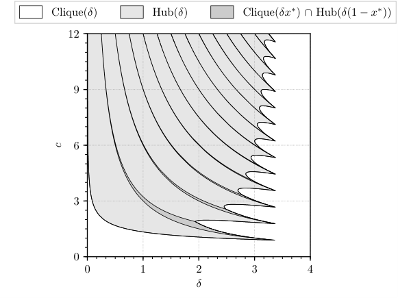
Note that Theorem 1.8 remains agnostic about the exact structure of the conditional model in the case where there are multiple minimisers to x↦ψr​(δ,n​pr−1,x)x\mapsto\psi_{r}(\delta,np^{r-1},x). However, it is not too difficult to show that for every rr, the set of (δ,c)∈(0,∞)2(\delta,c)\in(0,\infty)^{2} for which x↦ψr​(δ,c,x)x\mapsto\psi_{r}(\delta,c,x) has multiple minimisers has Lebesgue measure zero. Figure 2 gives a graphical representation of the assertion of Theorem 1.8 in the case where r=3r=3 and n​p2→cnp^{2}\to c. As the figure illustrates, the conditional model undergoes infinitely many phase transitions if δ2/3/2>δ/3\delta^{2/3}/2>\delta/3 (that is, δ<3.375\delta<3.375) and no phase transition at all if δ2/3/2<δ/3\delta^{2/3}/2<\delta/3.

Refer to caption
Figure 2. Asymptotic structure of Gn,pG_{n,p} conditioned upon the upper tail event UT(δ)={Xn,pK3⩾(1+δ)𝔼[Xn,pK3]}\UT(\delta)=\{X_{n,p}^{K_{3}}\geqslant(1+\delta)\e[X_{n,p}^{K_{3}}]\} when n​p2→cnp^{2}\to c as n→∞n\to\infty. In this conditional model, it is highly probable that we observe either Cliqueε⁡(δ)\Clique_{\varepsilon}(\delta), Hubε⁡(δ)\Hub_{\varepsilon}(\delta), or Cliqueε⁡(δ​x∗)∩Hubε⁡((1−δ)​x∗)\Clique_{\varepsilon}(\delta x^{*})\cap\Hub_{\varepsilon}((1-\delta)x^{*}) with x∗=3​⌊δ​c/3⌋/(δ​c)∈(0,1)x^{*}=3\lfloor\delta c/3\rfloor/(\delta c)\in(0,1), depending on the values of δ\delta and cc (all regions are open).

1.4. Organisation of the paper

In Section 2, we present a short and self-contained solution to the upper tail problem for triangle counts in Gn,pG_{n,p}. This section is somewhat redundant, since its content is just a special case of the more general Proposition 6.4. We include it in order to demonstrate our method in a simple setting that conveniently avoids many technical complications that arise in the general case.

Section 3 introduces a concentration inequality that gives a general condition under which the logarithmic upper tail probability can be approximated by ΦX​(δ)\Phi_{X}(\delta), the solution to the optimisation problem (2).

In Section 4, we use the inequality developed in Section 3 to determine the asymptotics of the logarithmic upper tail probability of XN,pk-APX_{N,p}^{\text{$k$-AP}} in the complete range of densities where localisation occurs. After collecting some graph-theoretic tools in Section 5, we study the localised regime of the upper tails of Xn,pKrX_{n,p}^{K_{r}} and Xn,pHX_{n,p}^{H} for connected, Δ\Delta-regular graphs HH in Sections 6 and 7, respectively. We note that the three Sections 4, 6, and 7 are logically independent and may be read in any order; however, both Sections 6 and 7 rely on the tools of Section 5.

In Section 8, we prove various results related to the Poisson regime; in particular, we give the proofs of Theorems 1.4 and 1.6. The arguments we use there do not rely on the methods developed in Section 3, but rather on explicit calculations of high factorial moments. Section 9 contains a brief discussion on extending the result from Section 3 to the more general case of nonnegative random variables on the hypercube. Finally, in Section 10 we make some concluding remarks and discuss open problems.

1.5. Notation

Before ending the introduction, we collect some notation which will be used throughout the paper. We write KrK_{r} for the complete graph on rr vertices and Ks,tK_{s,t} for the complete bipartite graph with parts of size ss and tt. For any graph GG, let V⁡(G)V(G) and E⁡(G)E(G) denote the vertex and edge sets of GG, respectively, and set vG=|V⁡(G)|v_{G}=|V(G)| and eG=|E⁡(G)|e_{G}=|E(G)|. For two graphs JJ and GG, we let N⁡(J,G)N(J,G) be the number of copies of JJ in GG, and Emb⁡(J,G)\Emb(J,G) be the set of embeddings of JJ into GG—i.e., injective maps from V⁡(J)V(J) to V⁡(G)V(G) that map edges of JJ to edges of GG. For an edge u​v∈E⁡(G)uv\in E(G), we also let N⁡(J,G,u​v)N(J,G;uv) and Emb⁡(J,G,u​v)\Emb(J,G;uv) be the number of copies of JJ that contain the edge u​vuv, and the set of embeddings that map an edge of JJ to u​vuv, respectively. Finally, for a subset II of ⟦N⟧\llbracket{N}\rrbracket, we let YI=∏i∈IYiY_{I}=\prod_{i\in I}Y_{i}, and 𝔼I​[X]=𝔼⁡[X∣YI=1]\mathbb{E}_{I}[X]=\mathbb{E}[X\mid Y_{I}=1]. If subsets I⊆⟦N⟧I\subseteq\llbracket{N}\rrbracket can be identified with subgraphs G⊆KnG\subseteq K_{n}, as in Example 1.2, we will write 𝔼G⁡[X]\e_{G}[X] instead of 𝔼I⁡[X]\e_{I}[X].

2. Triangles in random graphs

Assume that n−1​log⁡n≪p≪1n^{-1}\log n\ll p\ll 1 and let XX denote the number of triangles in Gn,pG_{n,p}. Using the shorthand notation 𝔼G⁡[X]=𝔼⁡[X∣G⊆Gn,p]\e_{G}[X]=\e[X\mid G\subseteq G_{n,p}], we define, for each positive δ\delta,

(6) ΦX​(δ)=min⁡{eG​log⁡(1/p):G⊆Kn​ and ​𝔼G​[X]⩾(1+δ)​𝔼⁡[X]}.\Phi_{X}(\delta)=\min{\big\{e_{G}\log(1/p):G\subseteq K_{n}\text{ and }\e_{G}[X]\geqslant(1+\delta)\e[X]\big\}}.

Note that this agrees with the definition (2). The goal of this section is to prove that, for every fixed positive ε\varepsilon and all large enough nn,

(7) (1−ε)​ΦX​(δ−ε)⩽−log⁡ℙ⁡(X⩾(1+δ)​𝔼⁡[X])⩽(1+ε)​ΦX​(δ+ε).(1-\varepsilon)\Phi_{X}(\delta-\varepsilon)\leqslant-\log\mathbb{P}\big(X\geqslant(1+\delta)\e[X]\big)\leqslant(1+\varepsilon)\Phi_{X}(\delta+\varepsilon).

At this point, we do not address the issue of evaluating ΦX​(δ)\Phi_{X}(\delta). For the sake of completeness, let us mention that a special case of a more general result of Lubetzky–Zhao [57] is that, when n−1≪p≪1n^{-1}\ll p\ll 1,

limn→∞ΦX​(δ)n2​p2​log⁡(1/p)={δ2/3/2if n​p2→0min⁡{δ/3,δ2/3/2}if n​p2→∞.\lim_{n\to\infty}\frac{\Phi_{X}(\delta)}{n^{2}p^{2}\log(1/p)}=\begin{cases}\delta^{2/3}/2&\text{if $np^{2}\to 0$}\\ \min\left\{\delta/3,\delta^{2/3}/2\right\}&\text{if $np^{2}\to\infty$.}\end{cases}

In Section 6, we shall fill in the gap at p=Θ(n−1/2)p=\Theta(n^{-1/2}) to obtain an asymptotic formula for ΦX​(δ)\Phi_{X}(\delta) in the full range of interest.

We now give a proof of (7), where we may assume without loss of generality that ε⩽δ/10\varepsilon\leqslant\delta/10. All statements that we make in this section should be understood to hold only for sufficiently large nn. We start with some easy observations. First, for every graph GG with O⁡(1)O(1) edges, we have 𝔼G⁡[X]−𝔼⁡[X]=O⁡(1+np2)≪(δ−2​ε)​𝔼⁡[X]\e_{G}[X]-\e[X]=O(1+np^{2})\ll(\delta-2\varepsilon)\e[X], and so ΦX​(δ−2​ε)≫log⁡(1/p)≫1\Phi_{X}(\delta-2\varepsilon)\gg\log(1/p)\gg 1. Second, the condition in (6) is satisfied when GG is a clique on (1+δ)1/3​n​p(1+\delta)^{1/3}np vertices, and therefore ΦX​(δ−ε)⩽(1+δ)2/3​n2​p2​log⁡(1/p)/2\Phi_{X}(\delta-\varepsilon)\leqslant(1+\delta)^{2/3}n^{2}p^{2}\log(1/p)/2.

The easier of the two inequalities in (7) is the upper bound. To prove it, let GG be a graph attaining the minimum in the definition of ΦX​(δ+ε)\Phi_{X}(\delta+\varepsilon) and let ℙG(⋅)=ℙ(⋅∣G⊆Gn,p)\mathbb{P}_{G}(\cdot)=\mathbb{P}(\cdot\mid G\subseteq G_{n,p}). Since XX never exceeds (n3)\binom{n}{3},

(1+δ+ε)​𝔼⁡[X]⩽𝔼G⁡[X]⩽(n3)​ℙG​(X⩾(1+δ)​𝔼⁡[X])+(1+δ)​𝔼⁡[X],(1+\delta+\varepsilon)\e[X]\leqslant\e_{G}[X]\leqslant\binom{n}{3}\mathbb{P}_{G}\big(X\geqslant(1+\delta)\e[X]\big)+(1+\delta)\e[X],

and so

ℙG​(X⩾(1+δ)​𝔼⁡[X])⩾ε​𝔼⁡[X]/(n3)=ε​p3.\mathbb{P}_{G}\big(X\geqslant(1+\delta)\e[X]\big)\geqslant\varepsilon\e[X]/\binom{n}{3}=\varepsilon p^{3}.

Hence,

−log⁡ℙ⁡(X⩾(1+δ)​𝔼⁡[X])⩽−log⁡(ℙ⁡(G⊆Gn,p)⋅ℙG​(X⩾(1+δ)​𝔼⁡[X]))⩽eG​log⁡(1/p)+log⁡(1/ε​p3).\begin{split}-\log\mathbb{P}\big(X\geqslant(1+\delta)\e[X]\big)&\leqslant-\log\Big(\mathbb{P}(G\subseteq G_{n,p})\cdot\mathbb{P}_{G}\big(X\geqslant(1+\delta)\e[X]\big)\Big)\\ &\leqslant e_{G}\log(1/p)+\log(1/\varepsilon p^{3}).\end{split}

Since eG​log⁡(1/p)=ΦX​(δ+ε)⩾ΦX​(δ−2​ε)≫log⁡(1/p)e_{G}\log(1/p)=\Phi_{X}(\delta+\varepsilon)\geqslant\Phi_{X}(\delta-2\varepsilon)\gg\log(1/p), this establishes the lower bound in (7).

We now turn to proving the lower bound. Let C=C⁡(ε,δ)C=C(\varepsilon,\delta) denote a sufficiently large positive constant. We call a graph G⊆KnG\subseteq K_{n} a seed if

  1. (S1)

    𝔼G⁡[X]⩾(1+δ−ε)​𝔼⁡[X]\e_{G}[X]\geqslant(1+\delta-\varepsilon)\e[X] and

  2. (S2)

    eG⩽C​n2​p2​log⁡(1/p)e_{G}\leqslant Cn^{2}p^{2}\log(1/p).

We make the following claim:

2.1.

ℙ(X⩾(1+δ)𝔼[X])⩽(1+ε)ℙ(Gn,p contains a seed)\mathbb{P}\big(X\geqslant(1+\delta)\e[X]\big)\leqslant(1+\varepsilon)\mathbb{P}\big(G_{n,p}\text{ contains a seed}\big).

2.2.

Given this claim, one may be tempted to simply apply the union bound over all seeds. Using such a strategy, one would find that

ℙ⁡(X⩾(1+δ)​𝔼⁡[X])\displaystyle\mathbb{P}\big(X\geqslant(1+\delta)\e[X]\big) ⩽Claim 2.1(1+ε)​ℙ​(Gn,p​ contains a seed)\displaystyle\stackrel{{\scriptstyle\text{Claim~\ref{cl:triaseed}}}}{{\leqslant}}(1+\varepsilon)\mathbb{P}\big(G_{n,p}\text{ contains a seed}\big)
(8) ⩽(1+ε)​∑m=mmin∞pm⋅|{G⊆Kn:G is a seed with m edges}|,\displaystyle\stackrel{{\scriptstyle\phantom{\text{Claim~\ref{cl:triaseed}}}}}{{\leqslant}}(1+\varepsilon)\sum_{m=m_{\min}}^{\infty}p^{m}\cdot|\{G\subseteq K_{n}:\text{$G$ is a seed with $m$ edges}\}|,

where mmin=ΦX​(δ−ε)/log⁡(1/p)m_{\min}=\Phi_{X}(\delta-\varepsilon)/\log(1/p) is the minimal number of edges in a seed. Unfortunately, such a strategy is bound to fail, as there are far too many seeds. To see this, we observe that if GG satisfies (S1), then so does any supergraph of GG. In particular, if we take a seed with mminm_{\min} edges and add an arbitrary set of K​mminKm_{\min} edges (where KK is a large constant), the resulting graph remains a seed. Therefore, we can (rather loosely) bound the number of seeds with m~=(K+1)​mmin\tilde{m}=(K+1)m_{\min} edges from below:

|{G⊆Kn:G is a seed with m~ edges}|⩾((n2)−mminK​mmin)⩾(13​(1+δ)2/3​K​p2)K​mmin,\displaystyle|\{G\subseteq K_{n}:\text{$G$ is a seed with $\tilde{m}$ edges}\}|\geqslant\binom{{\binom{n}{2}-m_{\min}}}{Km_{\min}}\geqslant\left(\frac{1}{3(1+\delta)^{2/3}Kp^{2}}\right)^{Km_{\min}},

using the bound (xy)⩾(x/2​y)y\binom{x}{y}\geqslant(x/2y)^{y} for any y<x/2y<x/2 and mmin⩽(1+δ)2/3​n2​p2/2m_{\min}\leqslant(1+\delta)^{2/3}n^{2}p^{2}/2. If we choose KK to be large enough, we may conclude that

|{G⊆Kn:G is a seed with m~ edges|⩾(1/p)3​m~/2,|\{G\subseteq K_{n}:\text{$G$ is a seed with $\tilde{m}$ edges}|\geqslant(1/p)^{3\tilde{m}/2},

for all large enough nn. This shows that the m~\tilde{m}th term of the final sum in (8) is arbitrarily large, making the entire approach fruitless.

From Remark 2.2, it is clear that seeds may include ‘extraneous’ edges that have no structural role in the upper tail event. We wish to consider more constrained structures which exclude constructions like the one outlined above. To that end, we call a graph G∗⊆KnG^{*}\subseteq K_{n} a core if

  1. (C1)

    𝔼G∗⁡[X]⩾(1+δ−2​ε)​𝔼⁡[X]\e_{G^{*}}[X]\geqslant(1+\delta-2\varepsilon)\e[X],

  2. (C2)

    eG∗⩽C​n2​p2​log⁡(1/p)e_{G^{*}}\leqslant Cn^{2}p^{2}\log(1/p), and

  3. (C3)

    mine∈E⁡(G∗)⁡(𝔼G∗⁡[X]−𝔼G∗∖e⁡[X])⩾ε​𝔼⁡[X]/(Cn2​p2​log⁡(1/p))\min_{e\in E({G^{*}})}\big(\e_{G^{*}}[X]-\e_{{G^{*}}\setminus e}[X]\big)\geqslant\varepsilon\e[X]/\big(Cn^{2}p^{2}\log(1/p)\big).

Condition (C3) requires that every edge contributed meaningfully to the expectation, and thus excludes the pathological seeds described above.

2.3.

Every seed contains a core.

Finally, we claim that the additional constraint (C3) allows us to get a very strong bound on the number of cores with a given number of edges, as it ensures that either the product of the degrees of the endpoints of any edge in G∗G^{*} must be nearly as large as eG∗e_{G^{*}}, or the sum of these degrees is nearly linear in nn (note that the former condition holds when G∗G^{*} is a clique, and the latter when G∗G^{*} is a hub). This, in turn, implies that the number of cores with a given set of vertices and mm edges is exp⁡(O⁡(m​log⁡log⁡(1/p))CLOSE\exp(O(m\log\log(1/p)). Once we show that the number of choices for the vertex set of a core with mm edges is (1/p)o⁡(m)(1/p)^{o(m)}, we prove the following claim.

2.4.

For every mm, there are at most (1/p)ε​m(1/p)^{\varepsilon m} cores with exactly mm edges.

As will be discussed in Section 3, we refer to the property described in Claim 2.4 as entropic stability.

Let us show how these three claims imply the lower bound in (7):

ℙ⁡(X⩾(1+δ)​𝔼⁡[X])⩽Claim 2.1(1+ε)​ℙ​(Gn,p​ contains a seed)⩽Claim 2.3(1+ε)​ℙ​(Gn,p​ contains a core)⩽Claim 2.2(1+ε)​∑m=0∞pm⋅|{G∗⊆Kn:G∗ is a core with m edges}|⩽Claim 2.4(1+ε)​∑m=mmin∞p(1−ε)​m,\begin{split}\mathbb{P}\big(X\geqslant(1+\delta)\e[X]\big)&\stackrel{{\scriptstyle\text{Claim~\ref{cl:triaseed}}}}{{\leqslant}}(1+\varepsilon)\mathbb{P}\big(G_{n,p}\text{ contains a seed}\big)\\ &\stackrel{{\scriptstyle\text{Claim~\ref{cl:triacore}}}}{{\leqslant}}(1+\varepsilon)\mathbb{P}\big(G_{n,p}\text{ contains a core}\big)\\ &\stackrel{{\scriptstyle\text{\phantom{Claim~2.2}}}}{{\leqslant}}(1+\varepsilon)\sum_{m=0}^{\infty}p^{m}\cdot|\{G^{*}\subseteq K_{n}:\text{$G^{*}$ is a core with $m$ edges}\}|\\ &\stackrel{{\scriptstyle\text{Claim~\ref{cl:triacorecount}}}}{{\leqslant}}(1+\varepsilon)\sum_{m=m_{\min}}^{\infty}p^{(1-\varepsilon)m},\end{split}

where mminm_{\min} is the minimal number of edges in a core. Since (C1) implies that ΦX​(δ−2​ε)⩽mmin⋅log⁡(1/p)\Phi_{X}(\delta-2\varepsilon)\leqslant m_{\min}\cdot\log(1/p), the assumption p≪1p\ll 1 yields

ℙ⁡(X⩾(1+δ)​𝔼⁡[X])⩽(1+2​ε)​exp⁡(−(1−ε)​ΦX​(δ−2​ε)).\mathbb{P}\big(X\geqslant(1+\delta)\e[X]\big)\leqslant(1+2\varepsilon)\exp\big(-(1-\varepsilon)\Phi_{X}(\delta-2\varepsilon)\big).

Finally, as ΦX​(δ−2​ε)≫1\Phi_{X}(\delta-2\varepsilon)\gg 1, we obtain

−log⁡ℙ⁡(X⩾(1+δ)​𝔼⁡[X])⩾(1−2​ε)​ΦX​(δ−2​ε),-\log\mathbb{P}\big(X\geqslant(1+\delta)\e[X]\big)\geqslant(1-2\varepsilon)\Phi_{X}(\delta-2\varepsilon),

thus proving (7) with 2​ε2\varepsilon instead of ε\varepsilon.

2.5.

Conditions (S2) and (C2) require both seeds and cores to have no more than C​n2​p2​log⁡(1/p)Cn^{2}p^{2}\log(1/p) edges, forcing us to consider graphs which are larger than the minimiser of ΦX​(δ)\Phi_{X}(\delta) by a multiplicative factor of log⁡(1/p)\log(1/p). This is optimal in the following sense. On the one hand, replacing log⁡(1/p)\log(1/p) with a larger function would weaken the conclusion of Claim 2.1 and make Claim 2.4 hold only for a smaller range of densities pp. On the other hand, if we could replace log⁡(1/p)\log(1/p) by ℓ⁡(p)=o⁡(log⁡(1/p))\ell(p)=o(\log(1/p)) without altering the validity of Claim 2.1, then Claim 2.4 (with an appropriately adjusted definition of a core) would hold for any p≫ℓ⁡(p)/np\gg\ell(p)/n; this would imply an upper bound on the upper tail probability that is stronger than the lower bound proven in Theorem 1.6 for ℓ⁡(p)/n≪p≪log⁡n/n\ell(p)/n\ll p\ll\log n/n.

Proof of Claim 2.1.

We refine a classical argument due to Janson, Oleszkiewicz, and Ruciński [44]. Let ZZ be the indicator random variable of the event that Gn,pG_{n,p} does not contain a seed and let ℓ=⌈(C/3)​n2​p2​log⁡(1/p)⌉\ell=\lceil(C/3)n^{2}p^{2}\log(1/p)\rceil. Since X​Z⩾0XZ\geqslant 0 and Zℓ=ZZ^{\ell}=Z, Markov’s inequality gives

(9) ℙ⁡(X⩾(1+δ)​𝔼⁡[X]​ and Gn,p contains no seed)=ℙ⁡(XZ⩾(1+δ)​𝔼⁡[X])⩽𝔼⁡[Xℓ​Z](1+δ)ℓ​𝔼⁡[X]ℓ.\mathbb{P}\big(X\geqslant(1+\delta)\e[X]\text{ and $G_{n,p}$ contains no seed}\big)=\mathbb{P}\big(XZ\geqslant(1+\delta)\e[X]\big)\leqslant\frac{\e[X^{\ell}Z]}{(1+\delta)^{\ell}\e[X]^{\ell}}.

We write X=∑TYTX=\sum_{T}Y_{T}, where the sum ranges over all triangles TT in KnK_{n} and YTY_{T} is the indicator random variable of the event that TT is contained in Gn,pG_{n,p}. For every subgraph G⊆KnG\subseteq K_{n}, let ZGZ_{G} be the indicator random variable of the event that G∩Gn,pG\cap G_{n,p} does not contain a seed. Observe that ZG′⩽ZGZ_{G^{\prime}}\leqslant Z_{G} whenever G⊆G′G\subseteq G^{\prime}. In particular, since Z=ZKnZ=Z_{K_{n}}, we have, for every k∈⟦ℓ⟧k\in\llbracket{\ell}\rrbracket,

𝔼⁡[Xk​Z]=∑T1,…,Tk𝔼⁡[YT1​⋯​YTk⋅Z]⩽∑T1,…,Tk𝔼⁡[YT1​⋯​YTk⋅ZT1∪⋯∪Tk]⩽∑T1,…,Tk−1𝔼⁡[YT1​⋯​YTk−1⋅ZT1∪⋯∪Tk−1]⋅∑Tk𝔼⁡[YTk∣YT1​…​YTk−1⋅ZT1∪⋯∪Tk−1=1],\begin{split}\e[X^{k}Z]&=\sum_{T_{1},\dotsc,T_{k}}\e[Y_{T_{1}}\dotsb Y_{T_{k}}\cdot Z]\\ &\leqslant\sum_{T_{1},\dotsc,T_{k}}\e[Y_{T_{1}}\dotsb Y_{T_{k}}\cdot Z_{T_{1}\cup\dotsb\cup T_{k}}]\\ &\leqslant\kern-5.0pt\sum_{T_{1},\dotsc,T_{k-1}}\kern-4.0pt\e[Y_{T_{1}}\dotsb Y_{T_{k-1}}\cdot Z_{T_{1}\cup\dotsb\cup T_{k-1}}]\cdot\sum_{T_{k}}\e[Y_{T_{k}}\mid Y_{T_{1}}\dotsc Y_{T_{k-1}}\cdot Z_{T_{1}\cup\dotsb\cup T_{k-1}}=1],\end{split}

where we can let the first sum in the last line range only over sequences T1,…,Tk−1T_{1},\dotsc,T_{k-1} for which the event {YT1⋯YTk−1⋅ZT1∪⋯∪Tk−1=1}\big\{Y_{T_{1}}\dotsb Y_{T_{k-1}}\cdot Z_{T_{1}\cup\dotsb\cup T_{k-1}}=1\big\} has positive probability. This is equivalent to saying that the graph T1∪⋯∪Tk−1T_{1}\cup\dotsb\cup T_{k-1} does not contain a seed and thus YT1​⋯​YTk−1⋅ZT1∪⋯∪Tk−1=YT1​⋯​YTk−1Y_{T_{1}}\dotsb Y_{T_{k-1}}\cdot Z_{T_{1}\cup\dotsb\cup T_{k-1}}=Y_{T_{1}}\dotsb Y_{T_{k-1}}. Moreover, since eT1∪⋯∪Tk−1⩽3​(k−1)⩽3​(ℓ−1)⩽C​n2​p2​log⁡(1/p)e_{T_{1}\cup\dotsb\cup T_{k-1}}\leqslant 3(k-1)\leqslant 3(\ell-1)\leqslant Cn^{2}p^{2}\log(1/p),

∑Tk𝔼⁡[YTk∣YT1​…​YTk−1=1]=𝔼T1∪⋯∪Tk−1⁡[X]<(1+δ−ε)​𝔼⁡[X],\sum_{T_{k}}\e[Y_{T_{k}}\mid Y_{T_{1}}\dotsc Y_{T_{k-1}}=1]=\e_{T_{1}\cup\dotsb\cup T_{k-1}}[X]<(1+\delta-\varepsilon)\e[X],

as otherwise T1∪⋯∪Tk−1T_{1}\cup\dotsb\cup T_{k-1} would be a seed, see (S1) and (S2). Therefore,

∑T1,…,Tk𝔼⁡[YT1​⋯​YTk⋅ZT1∪⋯∪Tk]<(1+δ−ε)​𝔼⁡[X]⋅∑T1,…,Tk−1𝔼⁡[YT1​⋯​YTk−1⋅ZT1∪⋯∪Tk−1]\sum_{T_{1},\dotsc,T_{k}}\e[Y_{T_{1}}\dotsb Y_{T_{k}}\cdot Z_{T_{1}\cup\dotsb\cup T_{k}}]<(1+\delta-\varepsilon)\e[X]\cdot\sum_{T_{1},\dotsc,T_{k-1}}\e[Y_{T_{1}}\dotsb Y_{T_{k-1}}\cdot Z_{T_{1}\cup\dotsb\cup T_{k-1}}]

and it follows by induction that 𝔼⁡[Xℓ​Z]<(1+δ−ε)ℓ​𝔼⁡[X]ℓ\e[X^{\ell}Z]<(1+\delta-\varepsilon)^{\ell}\e[X]^{\ell}. Substituting this inequality into (9) gives

ℙ⁡(X⩾(1+δ)​𝔼⁡[X]​ and Gn,p contains no seed)⩽(1+δ−ε1+δ)ℓ.\mathbb{P}\big(X\geqslant(1+\delta)\e[X]\text{ and $G_{n,p}$ contains no seed}\big)\leqslant\left(\frac{1+\delta-\varepsilon}{1+\delta}\right)^{\ell}.

Since the probability that Gn,pG_{n,p} contains a seed is at least e−ΦX​(δ−ε)e^{-\Phi_{X}(\delta-\varepsilon)}, the probability that Gn,pG_{n,p} contains a given seed of smallest size, the bounds 1≪ΦX​(δ−ε)⩽(1+δ)2/3​n2​p2​log⁡(1/p)/21\ll\Phi_{X}(\delta-\varepsilon)\leqslant(1+\delta)^{2/3}n^{2}p^{2}\log(1/p)/2 imply that, for all sufficiently large nn,

(1+δ−ε1+δ)ℓ⩽(1+δ−ε1+δ)(C/3)​n2​p2​log⁡(1/p)⩽ε​e−ΦX​(δ−ε)⩽ε​ℙ​(Gn,p contains a seed)\left(\frac{1+\delta-\varepsilon}{1+\delta}\right)^{\ell}\leqslant\left(\frac{1+\delta-\varepsilon}{1+\delta}\right)^{(C/3)n^{2}p^{2}\log(1/p)}\leqslant\varepsilon e^{-\Phi_{X}(\delta-\varepsilon)}\leqslant\varepsilon\mathbb{P}\big(\text{$G_{n,p}$ contains a seed}\big)

whenever the constant CC is sufficiently large44 4 We note that the requirement for CC to be large is only used here.. This implies the assertion of the claim. ∎

Proof of Claim 2.3.

Let GG be a seed. Define a sequence G=G0⊇G1⊇⋯⊇Gs=G∗G=G_{0}\supseteq G_{1}\supseteq\dotsb\supseteq G_{s}=G^{*} of subgraphs of GG by repeatedly setting Gi+1=Gi∖eG_{i+1}=G_{i}\setminus e for some edge e∈Gie\in G_{i} such that 𝔼Gi−𝔼Gi∖e⁡[X]<ε​𝔼⁡[X]/(Cn2​p2​log⁡(1/p))\e_{G_{i}}-\e_{G_{i}\setminus e}[X]<\varepsilon\e[X]/\big(Cn^{2}p^{2}\log(1/p)\big), as long as such an edge ee exists. By construction, G∗G^{*} clearly satisfies (C3). Since eG∗⩽eG⩽C​n2​p2​log⁡(1/p)e_{G^{*}}\leqslant e_{G}\leqslant Cn^{2}p^{2}\log(1/p), we see that (C2) holds as well. Finally, as s⩽eG⩽C​n2​p2​log⁡(1/p)s\leqslant e_{G}\leqslant Cn^{2}p^{2}\log(1/p), we have

𝔼G⁡[X]−𝔼G∗⁡[X]=∑i=0s−1(𝔼Gi⁡[X]−𝔼Gi+1⁡[X])<ε​𝔼⁡[X].\e_{G}[X]-\e_{G^{*}}[X]=\sum_{i=0}^{s-1}\big(\e_{G_{i}}[X]-\e_{G_{i+1}}[X]\big)<\varepsilon\e[X].

Since GG is a seed, 𝔼G⁡[X]⩾(1+δ−ε)​𝔼⁡[X]\e_{G}[X]\geqslant(1+\delta-\varepsilon)\e[X] and we obtain (C1). ∎

Proof of Claim 2.4.
eeG∗G^{*}BG∗B_{G^{*}}AG∗A_{G^{*}}G∗G^{*}
Figure 3. Left: The sets AG∗A_{G^{*}} and BG∗B_{G^{*}} of high-degree vertices capture the edges of the core. Right: Three different types of triangles containing an edge ee in the core G∗G^{*}.

We bound the number of cores with mm edges from above. This number is zero whenever m>C​n2​p2​log⁡(1/p)m>Cn^{2}p^{2}\log(1/p), by (C2). We may thus assume that m⩽C​n2​p2​log⁡(1/p)m\leqslant Cn^{2}p^{2}\log(1/p). Given a core G∗{G^{*}}, we denote by AG∗A_{G^{*}} the set of vertices of G∗{G^{*}} with degree at least ε​n​p/(30​C​log⁡(1/p))\varepsilon np/\big(30C\log(1/p)\big) and by BG∗⊆AG∗B_{G^{*}}\subseteq A_{G^{*}} the set of vertices of G∗{G^{*}} with degree at least ε​n/(30​C​log⁡(1/p))\varepsilon n/\big(30C\log(1/p)\big), where the degree is taken in G∗G^{*}. Since G∗G^{*} has mm edges,

|AG∗|⩽a:=60​C​m​log⁡(1/p)ε​n​pand|BG∗|⩽b:=60​C​m​log⁡(1/p)ε​n.|A_{G^{*}}|\leqslant a:=\frac{60Cm\log(1/p)}{\varepsilon np}\quad\text{and}\quad|B_{G^{*}}|\leqslant b:=\frac{60Cm\log(1/p)}{\varepsilon n}.

The key observation, which we will now verify, is that every edge of G∗{G^{*}} is either contained in AG∗A_{G^{*}} or has an endpoint in BG∗B_{G^{*}}, see Figure 3 for an illustration. To see this, consider some edge e∈E⁡(G∗)e\in E(G^{*}). For every nonempty graph F⊆K3F\subseteq K_{3}, let N⁡(F,G∗,e)N(F,G^{*};e) denote the number of copies of FF in G∗G^{*} that contain ee. By considering how the n−2n-2 triangles in KnK_{n} that contain ee intersect G∗G^{*} (see Figure 3), one can see that

𝔼G∗⁡[X]−𝔼G∗∖e⁡[X]⩽(N⁡(K3,G∗,e)+N⁡(K1,2,G∗,e)⋅p+np2)⋅(1−p).\e_{G^{*}}[X]-\e_{G^{*}\setminus e}[X]\leqslant\big(N(K_{3},G^{*};e)+N(K_{1,2},G^{*};e)\cdot p+np^{2}\big)\cdot(1-p).

Using 𝔼G∗⁡[X]−𝔼G∗∖e⁡[X]⩾ε​𝔼⁡[X]/(Cn2​p2​log⁡(1/p))\e_{G^{*}}[X]-\e_{G^{*}\setminus e}[X]\geqslant\varepsilon\e[X]/(Cn^{2}p^{2}\log(1/p)) and 𝔼⁡[X]⩾(1−o⁡(1))​n3​p3/6\e[X]\geqslant(1-o(1))n^{3}p^{3}/6, we thus get

ε​n​p7​C​log⁡(1/p)⩽N⁡(K3,G∗,e)+N⁡(K1,2,G∗,e)⋅p+n​p2.\frac{\varepsilon np}{7C\log(1/p)}\leqslant N(K_{3},G^{*};e)+N(K_{1,2},G^{*};e)\cdot p+np^{2}.

Since p≪1p\ll 1 implies that n​p2≪n​p/log⁡(1/p)np^{2}\ll np/\log(1/p), we find that either

(10) N⁡(K3,G∗,e)⩾ε​n​p15​C​log⁡(1/p)orN⁡(K1,2,G∗,e)⩾ε​n15​C​log⁡(1/p).N(K_{3},G^{*};e)\geqslant\frac{\varepsilon np}{15C\log(1/p)}\quad\text{or}\quad N(K_{1,2},G^{*};e)\geqslant\frac{\varepsilon n}{15C\log(1/p)}.

Since N⁡(K3,G∗,u​v)⩽min⁡{degG∗⁡u,degG∗⁡v}N(K_{3},G^{*};uv)\leqslant\min\{\deg_{G^{*}}u,\deg_{G^{*}}v\} and N⁡(K1,2,G∗,u​v)⩽degG∗⁡u+degG∗⁡vN(K_{1,2},G^{*};uv)\leqslant\deg_{G^{*}}u+\deg_{G^{*}}v, the first inequality in (10) implies that ee is contained in AG∗A_{G^{*}} whereas the second inequality implies that ee has an endpoint in BG∗B_{G^{*}}, as claimed.

Our key observation implies that for fixed sets B⊆A⊆⟦n⟧B\subseteq A\subseteq\llbracket{n}\rrbracket with |A|=a|A|=a and |B|=b|B|=b, there are at most (a2/2+b​nm)\binom{a^{2}/2+bn}{m} cores G∗{G^{*}} with mm edges that satisfy AG∗⊆AA_{{G^{*}}}\subseteq A and BG∗⊆BB_{{G^{*}}}\subseteq B. We can thus (generously) upper bound the number of cores with mm edges by

(na)​(nb)​(a2/2+b​nm).\binom{n}{a}\binom{n}{b}\binom{a^{2}/2+bn}{m}.

Recalling the inequality (xy)⩽(e​x/y)y\binom{x}{y}\leqslant(ex/y)^{y}, valid for all nonnegative integers xx and yy, we may conclude that the number of cores with mm edges is at most

n120​C​m​log⁡(1/p)ε​n​p⋅(e​(60​C)2​m​(log⁡(1/p))22​ε2​n2​p2+e​60​C​log⁡(1/p)ε)m.n^{\frac{120Cm\log(1/p)}{\varepsilon np}}\cdot\left(\frac{e(60C)^{2}m\big(\log(1/p)\big)^{2}}{2\varepsilon^{2}n^{2}p^{2}}+\frac{e60C\log(1/p)}{\varepsilon}\right)^{m}.

Since p≫n−1​log⁡np\gg n^{-1}\log n, the first factor is at most eo⁡(m​log⁡(1/p))e^{o(m\log(1/p))}. Using m⩽C​n2​p2​log⁡(1/p)m\leqslant Cn^{2}p^{2}\log(1/p), the second factor is at most eO⁡(m​log⁡log​(1/p))=eo⁡(m​log⁡(1/p))e^{O(m\log\log(1/p))}=e^{o(m\log(1/p))}. This shows that the number of cores with mm edges is indeed at most (1/p)ε​m(1/p)^{\varepsilon m}, as claimed. ∎

3. The main technical result: ‘entropic stability implies localisation’

The goal of this section is to state a general result that allows one, in many cases of interest, to reduce the problem of determining the precise asymptotics of the logarithmic upper tail probability of a polynomial (with nonnegative coefficients) of independent Bernoulli random variables to a counting problem. Since the main technical lemmas also apply to non-product measures on the hypercube, we phrase the basic definitions in this broader context.

We denote by YY a random variable taking values in the discrete NN-dimensional cube {0,1}N\{0,1\}^{N} and by X=X⁡(Y)X=X(Y) a real-valued, increasing function of YY with positive expectation. Given a subset I⊆⟦N⟧I\subseteq\llbracket{N}\rrbracket, we write YI=∏i∈IYiY_{I}=\prod_{i\in I}Y_{i} for the indicator random variable of the event {Yi=1 for all i∈I}\big\{Y_{i}=1\text{ for all }i\in I\big\}. Using the shorthand notation 𝔼I⁡[X]=𝔼⁡[X∣YI=1]\e_{I}[X]=\e[X\mid Y_{I}=1],55 5 Strictly speaking, 𝔼I⁡[X]\Ex_{I}[X] is well defined only if ℙ⁡(YI=1)>0\mathbb{P}(Y_{I}=1)>0. However, the value of 𝔼I⁡[X]\e_{I}[X] for sets II with ℙ⁡(YI=1)=0\mathbb{P}(Y_{I}=1)=0 does not affect any of our statements. we define a function ΦX:ℝ→ℝ⩾0∪{∞}\Phi_{X}\colon\mathbb{R}\to\mathbb{R}_{\geqslant 0}\cup\{\infty\} by66 6 We use the standard convention that min⁡∅=∞\min\varnothing=\infty.

(11) ΦX​(δ)=min⁡{−log⁡ℙ⁡(YI=1):I⊆⟦N⟧​ and ​𝔼I​[X]⩾(1+δ)​𝔼⁡[X]}.\Phi_{X}(\delta)=\min\big\{-\log\mathbb{P}(Y_{I}=1):I\subseteq\llbracket{N}\rrbracket\text{ and }\e_{I}[X]\geqslant(1+\delta)\e[X]\big\}.

It is easy to see that ΦX\Phi_{X} is a nondecreasing function satisfying ΦX​(δ)>0\Phi_{X}(\delta)>0 for all δ>0\delta>0. We say that a function X:{0,1}N→ℝ⩾0X\colon\{0,1\}^{N}\to\mathbb{R}_{\geqslant 0} is a polynomial with nonnegative coefficients and degree at most dd if it admits a representation X=∑I⊆⟦N⟧αI​YIX=\sum_{I\subseteq\llbracket{N}\rrbracket}\alpha_{I}Y_{I}, where each coefficient αI\alpha_{I} is nonnegative and αI=0\alpha_{I}=0 whenever |I|>d|I|>d.

Let ℐ\mathcal{I} be a collection of subsets I⊂⟦N⟧I\subset\llbracket{N}\rrbracket. Given ε>0\varepsilon>0 and p>0p>0, we say that ℐ\mathcal{I} is an entropically stable family (with respect to ε\varepsilon and pp) if, for every integer mm,

|{I∈ℐ:|I|=m}|⩽(1/p)ε​m/2.|\{I\in\mathcal{I}:|I|=m\}|\leqslant(1/p)^{\varepsilon m/2}.

For the sake of brevity, we will suppress the dependence of this property on ε\varepsilon and pp.

The following statement is the main technical result of our work.

3.1.

For every positive integer dd and all positive real numbers ε\varepsilon and δ\delta with ε<1/2\varepsilon<1/2, there is a positive K=K⁡(d,ε,δ)K=K(d,\varepsilon,\delta) such that the following holds. Let YY be a sequence of NN independent Ber⁡(p)\mathrm{Ber}(p) random variables for some p∈(0,1−ε]p\in(0,1-\varepsilon] and let X=X⁡(Y)X=X(Y) be a nonzero polynomial with nonnegative coefficients and degree at most dd such that ΦX​(δ−ε)⩾K​log⁡(1/p)\Phi_{X}(\delta-\varepsilon)\geqslant K\log(1/p). Denote by ℐ∗\mathcal{I}^{*} the collection of all subsets I⊆⟦N⟧I\subseteq\llbracket{N}\rrbracket satisfying

  1. (C1)

    𝔼I⁡[X]⩾(1+δ−ε)​𝔼⁡[X]\e_{I}[X]\geqslant(1+\delta-\varepsilon)\e[X],

  2. (C2)

    |I|⩽K⋅ΦX​(δ+ε)|I|\leqslant K\cdot\Phi_{X}(\delta+\varepsilon), and

  3. (C3)

    mini∈I⁡(𝔼I⁡[X]−𝔼I∖{i}⁡[X])⩾𝔼⁡[X]/(K⋅ΦX​(δ+ε))\min_{i\in I}\left(\e_{I}[X]-\e_{I\setminus\{i\}}[X]\right)\geqslant\e[X]/\big(K\cdot\Phi_{X}(\delta+\varepsilon)\big),

and assume ℐ∗\mathcal{I}^{*} is an entropically stable family. Then

(12) (1−ε)​ΦX​(δ−ε)⩽−log⁡ℙ⁡(X⩾(1+δ)​𝔼⁡[X])⩽(1+ε)​ΦX​(δ+ε)(1-\varepsilon)\Phi_{X}(\delta-\varepsilon)\leqslant-\log\mathbb{P}\big(X\geqslant(1+\delta)\e[X]\big)\leqslant(1+\varepsilon)\Phi_{X}(\delta+\varepsilon)

and, writing 𝒥∗\mathcal{J}^{*} for the collection of those I∈ℐ∗I\in\mathcal{I}^{*} with −log⁡ℙ⁡(YI=1)⩽(1+ε)​ΦX​(δ+ε)-\log\mathbb{P}(Y_{I}=1)\leqslant(1+\varepsilon)\Phi_{X}(\delta+\varepsilon),

(13) ℙ⁡(X⩾(1+δ)​𝔼⁡[X]​ and YI=0 for all I∈𝒥∗)⩽ε​ℙ​(X⩾(1+δ)​𝔼⁡[X]).\mathbb{P}\big(X\geqslant(1+\delta)\e[X]\text{ and $Y_{I}=0$ for all $I\in\mathcal{J}^{*}$}\big)\leqslant\varepsilon\mathbb{P}\big(X\geqslant(1+\delta)\e[X]\big).
3.2.

Observe that (12) gives tight bounds on the logarithmic upper tail probability of XX, provided that ΦX​(δ)=(I⁡(δ)+o⁡(1))​f​(N,p)\Phi_{X}(\delta)=\big(I(\delta)+o(1)\big)f(N,p) for a continuous, positive function II and some function ff. Equation (13) states that the upper tail event is (almost) contained in the event that YI=1Y_{I}=1 for some I∈𝒥∗I\in\mathcal{J}^{*}; note that each such II is a near-minimiser of ΦX​(δ−ε)\Phi_{X}(\delta-\varepsilon). In some cases, it is possible to classify these near-minimisers and thereby obtain a rough structural characterisation of the upper tail event.

3.3.

The assumption ΦX​(δ−ε)⩾K​log⁡(1/p)\Phi_{X}(\delta-\varepsilon)\geqslant K\log(1/p) means that conditioning on YI=1Y_{I}=1 for any constant-size subset I⊆⟦N⟧I\subseteq\llbracket{N}\rrbracket cannot increase the expected value of XX by more than (δ−ε)​𝔼⁡[X](\delta-\varepsilon)\e[X]; it is very easy to verify this for the applications we have in mind. The more onerous task is verifying that ℐ∗\mathcal{I}^{*} is an entropically stable family. In fact, a large part of this paper is dedicated to counting cores (as we call the elements of ℐ∗\mathcal{I}^{*}). Frequently, there are very few minimisers of ΦX​(δ)\Phi_{X}(\delta), for every δ>0\delta>0. Entropic stability quantifies the notion that there are few near-minimisers as well.

3.4.

In the following sections, we will compute the logarithmic upper tail probabilities in various settings by estimating the function ΦX\Phi_{X} and verifying that the random variable XX in question satisfies the assumptions of Theorem 3.1. As will be seen in the proof of Theorem 3.1, entropic stability implies that

(14) −log⁡ℙ⁡(YI∗=1​ for some ​I∗∈ℐ∗)⩾(1−ε/2)⋅ΦX​(δ−ε).-\log\mathbb{P}\left(Y_{I^{*}}=1\text{ for some }I^{*}\in\mathcal{I}^{*}\right)\geqslant(1-\varepsilon/2)\cdot\Phi_{X}(\delta-\varepsilon).

However, there are many natural contexts where the entropic stability assumption fails despite the fact that (14) remains true. For example, when H=C4H=C_{4}, then every copy of the complete bipartite graph K2,c​n2​p2K_{2,cn^{2}p^{2}} in KnK_{n} is a core, provided that cc is large enough. There are (nc​n2​p2)\binom{n}{cn^{2}p^{2}} such copies in KnK_{n} and (nc​n2​p2)\binom{n}{cn^{2}p^{2}} is larger than (1/p)Ω⁡(n2​p2)(1/p)^{\Omega(n^{2}p^{2})} when p≪n−1/2−ξp\ll n^{-1/2-\xi} for some small ξ>0\xi>0. In order to study such scenarios, one may search out a weaker condition which still implies (14), and employ Theorem 3.1 mutatis mutandis. One such modification is to allow the number of cores with mm edges to be as large as (1/p)m−mmin+o⁡(mmin)(1/p)^{m-m_{\min}+o(m_{\min})}; such a generalisation was introduced in the work of Basak–Basu [8].

3.5.

Let ℳ⁡({0,1}N)\mathcal{M}(\{0,1\}^{N}) be the set of measures on the NN-dimensional hypercube. For any random variable X=X⁡(Y)X=X(Y) defined on the pp-biased hypercube, it is possible to give an abstract description of the probability of the upper tail event via the Gibbs variational principle, which states that

−log⁡ℙ⁡(X⩾(1+δ)​𝔼⁡[X])⩾infν∈ℳδXDKL​(ν∥μp),-\log\mathbb{P}\left(X\geqslant(1+\delta)\Ex[X]\right)\geqslant\inf_{\nu\in\mathcal{M}_{\delta}^{X}}D_{\text{KL}}(\nu\mathrel{\|}\mu_{p}),

where μp\mu_{p} is the product of NN Bernoulli measures of mean pp, DKL(⋅∥⋅)D_{\text{KL}}(\cdot\mathrel{\|}\cdot) is the relative entropy

DKL​(ν∥μ)=∑y∈{0,1}Nν⁡(y)​log⁡(ν⁡(y)μ⁡(y)),D_{\text{KL}}(\nu\mathrel{\|}\mu)=\sum_{y\in\{0,1\}^{N}}\nu(y)\log\left(\frac{\nu(y)}{\mu(y)}\right),

and

ℳδX:={ν∈ℳ⁡({0,1}N):∑y∈{0,1}NX⁡(y)​ν​(y)⩾(1+δ)​𝔼⁡[X]}.\mathcal{M}_{\delta}^{X}:=\Big\{\nu\in\mathcal{M}(\{0,1\}^{N}):\sum_{y\in\{0,1\}^{N}}X(y)\nu(y)\geqslant(1+\delta)\Ex[X]\Big\}.

The naïve mean field approximation holds for the upper tail of XX if one can replace the infimum over all measures in ℳδX\mathcal{M}_{\delta}^{X} by an infimum over all product measures in ℳδX\mathcal{M}_{\delta}^{X}, while incurring only lower order errors.

The seminal work of Chatterjee–Dembo [17], further developed by Eldan [30] and Augeri [3], provides very general sufficient conditions that imply the naïve mean field approximation for a general function ff of Bernoulli random variables, stated in terms of the ‘smoothness’ of ff and the ‘complexity’ of its gradient. Although the various works consider different notions of low complexity, all of them seem to imply the heuristic statement that the set of all directions of the gradient of ff is an extremely sparse subset of the (N−1)(N-1)-dimensional sphere. An alternate approach to the naïve mean field approximation is used by Cook–Dembo [24], which specializes to the case of subgraph counts in Erdős–Rényi random graphs. Instead of appealing to gradient complexity bounds, they construct an efficient covering of (most of) the hypercube by convex sets on which the subgraph counts are nearly constant, in the spirit of the regularity-based approach of Chatterjee–Varadhan [21].

Although its formulation is rather different, Theorem 3.1 can also be considered in the context of the naïve mean field approximation, coverings of the hypercube, and low-complexity gradients. Given a subset I⊆⟦N⟧I\subseteq\llbracket{N}\rrbracket, we define a product measure νI\nu_{I} by

νI​(Yi=1)={1if i∈I,potherwise.\nu_{I}(Y_{i}=1)=\begin{cases}1&\text{if $i\in I$,}\\ p&\text{otherwise}.\end{cases}

A straightforward computation shows that DKL​(νI∥μp)=|I|​log⁡(1/p)D_{\text{KL}}(\nu_{I}\mathrel{\|}\mu_{p})=|I|\log(1/p), and so

ΦX​(δ)=inf{DKL​(νI∥μp):νI∈ℳδX}.\Phi_{X}(\delta)=\inf\big\{D_{\text{KL}}(\nu_{I}\mathrel{\|}\mu_{p}):\nu_{I}\in\mathcal{M}_{\delta}^{X}\big\}.

In these terms, Theorem 3.1 shows that, if ℐ∗\mathcal{I}^{*} an entropically stable family, then a particularly simple form of the naïve mean field approximation holds: one must only consider product measures that assign edges probability pp or 11. Our adaptation of the high moment argument of Janson, Oleszkiewicz, and Ruciński, used in Lemma 3.7, constructs a covering of (most of) the upper tail event by a family ℐ\mathcal{I} of small subsets II with νI∈ℳδX\nu_{I}\in\mathcal{M}_{\delta}^{X}. The extraction of cores from these subsets corresponds to identifying the directions in which the possible partial derivatives are large; in this perspective, entropic stability is analogous to the sparseness property that is encoded by the low-complexity gradient condition.

The final stipulation of Theorem 9.1 gives a structural description of the measure conditioned on the upper tail event. More specifically, a sample from the conditional measure will contain an element of 𝒥∗\mathcal{J}^{*} with high probability. Working from the naïve mean-field approximation, one may consider the more subtle question of the exact relationship between the conditional measure and the family of product measures in ℳδX\mathcal{M}_{\delta}^{X} that attain the minimal relative entropy from μp\mu_{p}. The work of Eldan–Gross [31] shows that, under certain conditions, the conditional measure is close to a mixture of such product measures, in the sense of optimal transport; Austin [4] proves similar results for a broader class of measures (not necessarily on the hypercube).

The upper bound on −log⁡ℙ⁡(X⩾(1+δ)​𝔼⁡[X])-\log\mathbb{P}\big(X\geqslant(1+\delta)\e[X]\big) stated in (12) will follow easily from the following simple lemma.

3.6.

Let YY be a random variable taking values in {0,1}N\{0,1\}^{N} and let X=X⁡(Y)X=X(Y) be a real-valued function of YY. Suppose that 𝔼⁡[X]>0\Ex[X]>0 and that X⩽MX\leqslant M always. Then for all positive ε\varepsilon and δ\delta,

−log⁡ℙ⁡(X⩾(1+δ)​𝔼⁡[X])⩽ΦX​(δ+ε)+log⁡(Mε​𝔼⁡[X]).-\log\mathbb{P}\big(X\geqslant(1+\delta)\e[X]\big)\leqslant\Phi_{X}(\delta+\varepsilon)+\log\left(\frac{M}{\varepsilon\e[X]}\right).
Proof.

Let t=(1+δ)​𝔼⁡[X]t=(1+\delta)\e[X]. If ΦX​(δ+ε)=∞\Phi_{X}(\delta+\varepsilon)=\infty, then the assertion of the lemma is vacuous. Otherwise, there exists a set I⊆⟦N⟧I\subseteq\llbracket{N}\rrbracket with −log⁡ℙ⁡(YI=1)=ΦX​(δ+ε)-\log{\mathbb{P}(Y_{I}=1)}=\Phi_{X}(\delta+\varepsilon) and 𝔼I⁡[X]⩾t+ε​𝔼⁡[X]\e_{I}[X]\geqslant t+\varepsilon\e[X]. As 𝔼I⁡[X]⩽M⋅ℙ⁡(X⩾t∣YI=1)+t\e_{I}[X]\leqslant M\cdot\mathbb{P}(X\geqslant t\mid Y_{I}=1)+t, it follows that

ℙ⁡(X⩾t)⩾ℙ⁡(YI=1)⋅ℙ⁡(X⩾t∣YI=1)⩾ℙ⁡(YI=1)⋅ε​𝔼⁡[X]M.\mathbb{P}(X\geqslant t)\geqslant\mathbb{P}(Y_{I}=1)\cdot\mathbb{P}(X\geqslant t\mid Y_{I}=1)\geqslant\mathbb{P}(Y_{I}=1)\cdot\frac{\varepsilon\e[X]}{M}.

Taking the negative logarithm of both sides gives the assertion of the lemma. ∎

The next lemma lies at the heart of the matter. In very broad terms, it states that the upper tail event {X⩾(1+δ)𝔼[X]}\big\{X\geqslant(1+\delta)\Ex[X]\big\}, viewed as a subset of the cube {0,1}N\{0,1\}^{N}, may be covered almost completely by a union of subcubes of small codimension, where, crucially, the average value of XX on each of these subcubes is at least (1+δ−ε)​𝔼⁡[X](1+\delta-\varepsilon)\Ex[X]. The proof uses a variant of the moment argument of Janson, Oleszkiewicz, and Ruciński [44].

3.7.

Let YY be a random variable taking values in {0,1}N\{0,1\}^{N} and let X=X⁡(Y)X=X(Y) be a nonzero polynomial with nonnegative coefficients and degree at most dd. Then for every positive integer ℓ\ell and all positive real numbers ε\varepsilon and δ\delta,

ℙ⁡(X⩾(1+δ)​𝔼⁡[X]​ and ​YI=0​ for all I∈ℐ)⩽(1+δ−ε1+δ)ℓ,\mathbb{P}\big(X\geqslant(1+\delta)\e[X]\text{ and }Y_{I}=0\text{ for all $I\in\mathcal{I}$}\big)\leqslant\left(\frac{1+\delta-\varepsilon}{1+\delta}\right)^{\ell},

where ℐ={I⊆⟦N⟧:|I|⩽d​ℓ​ and ​𝔼I​[X]⩾(1+δ−ε)​𝔼⁡[X]}\mathcal{I}=\big\{I\subseteq\llbracket{N}\rrbracket:|I|\leqslant d\ell\text{ and }\e_{I}[X]\geqslant(1+\delta-\varepsilon)\e[X]\big\}.

Proof.

Given S⊆⟦N⟧S\subseteq\llbracket{N}\rrbracket, let ZSZ_{S} be the indicator random variable of the event that YI=0Y_{I}=0 for all I∈ℐI\in\mathcal{I} with I⊆SI\subseteq S. Note that I′⊆II^{\prime}\subseteq I implies ZI⩽ZI′Z_{I}\leqslant Z_{I^{\prime}} and let Z=Z⟦N⟧Z=Z_{\llbracket{N}\rrbracket}. Since X​Z⩾0XZ\geqslant 0 and Zℓ=ZZ^{\ell}=Z, Markov’s inequality gives

(15) ℙ⁡(X⩾(1+δ)​𝔼⁡[X]​ and ​Z=1)=ℙ⁡(XZ⩾(1+δ)​𝔼⁡[X])⩽𝔼⁡[Xℓ​Z]((1+δ)​𝔼⁡[X])ℓ.\mathbb{P}\big(X\geqslant(1+\delta)\e[X]\text{ and }Z=1\big)=\mathbb{P}\big(XZ\geqslant(1+\delta)\e[X]\big)\leqslant\frac{\e[X^{\ell}Z]}{\big((1+\delta)\e[X]\big)^{\ell}}.

Write X=∑IαI​YIX=\sum_{I}\alpha_{I}Y_{I}, where the sum ranges over all subsets I⊆⟦N⟧I\subseteq\llbracket{N}\rrbracket, each coefficient αI\alpha_{I} is nonnegative, and αI=0\alpha_{I}=0 unless |I|⩽d|I|\leqslant d. Then for every k∈⟦ℓ⟧k\in\llbracket{\ell}\rrbracket,

𝔼⁡[Xk​Z]=∑I1,…,IkαI1​⋯​αIk​𝔼⁡[YI1​⋯​YIk⋅Z]⩽∑I1,…,IkαI1​⋯​αIk​𝔼⁡[YI1​⋯​YIk⋅ZI1∪⋯∪Ik]⩽∑I1,…,Ik−1αI1​⋯​αIk−1​𝔼⁡[YI1​⋯​YIk−1⋅ZI1∪⋯∪Ik−1]⋅𝔼⁡[X∣YI1​⋯​YIk−1⋅ZI1∪⋯∪Ik−1=1],\begin{split}\e[X^{k}Z]&=\sum_{I_{1},\dotsc,I_{k}}\alpha_{I_{1}}\dotsb\alpha_{I_{k}}\e[Y_{I_{1}}\dotsb Y_{I_{k}}\cdot Z]\\ &\leqslant\sum_{I_{1},\dotsc,I_{k}}\alpha_{I_{1}}\dotsb\alpha_{I_{k}}\e[Y_{I_{1}}\dotsb Y_{I_{k}}\cdot Z_{I_{1}\cup\dotsb\cup I_{k}}]\\ &\leqslant\kern-5.0pt\sum_{I_{1},\dotsc,I_{k-1}}\kern-6.0pt\alpha_{I_{1}}\dotsb\alpha_{I_{k-1}}\e[Y_{I_{1}}\dotsb Y_{I_{k-1}}\cdot Z_{I_{1}\cup\dotsb\cup I_{k-1}}]\cdot\e[X\mid Y_{I_{1}}\dotsb Y_{I_{k-1}}\cdot Z_{I_{1}\cup\dotsb\cup I_{k-1}}=1],\end{split}

where we may let the third sum range only over sequences I1,…,Ik−1I_{1},\dotsc,I_{k-1} for which the event {YI1⋯YIk−1⋅ZI1∪⋯∪Ik−1=1}\big\{Y_{I_{1}}\dotsb Y_{I_{k-1}}\cdot Z_{I_{1}\cup\dotsb\cup I_{k-1}}=1\big\} has a positive probability of occurring. Note that for any such sequence, YI1​⋯​YIk−1⋅ZI1∪⋯∪Ik−1=YI1​⋯​YIk−1Y_{I_{1}}\dotsb Y_{I_{k-1}}\cdot Z_{I_{1}\cup\dotsb\cup I_{k-1}}=Y_{I_{1}}\dotsb Y_{I_{k-1}} and I1∪⋯∪Ik−1∉ℐI_{1}\cup\dotsb\cup I_{k-1}\notin\mathcal{I}. Since |I1∪⋯∪Ik−1|⩽d⁡(k−1)⩽d​ℓ|I_{1}\cup\dotsb\cup I_{k-1}|\leqslant d(k-1)\leqslant d\ell, we have

𝔼⁡[X∣YI1​⋯​YIk−1=1]=𝔼I1∪⋯∪Ik⁡[X]<(1+δ−ε)​𝔼⁡[X],\e[X\mid Y_{I_{1}}\dotsb Y_{I_{k-1}}=1]=\e_{I_{1}\cup\dotsb\cup I_{k}}[X]<(1+\delta-\varepsilon)\e[X],

as otherwise I1∪⋯∪Ik−1I_{1}\cup\dotsb\cup I_{k-1} would belong to ℐ\mathcal{I}. It follows that

∑I1,…,IkαI1​⋯​αIk​𝔼⁡[YI1​⋯​YIk⋅ZI1∪⋯∪Ik]<(1+δ−ε)​𝔼⁡[X]⋅∑I1,…,Ik−1αI1​⋯​αIk−1​𝔼⁡[YI1​⋯​YIk−1⋅ZI1∪⋯∪Ik−1].\sum_{I_{1},\dotsc,I_{k}}\alpha_{I_{1}}\dotsb\alpha_{I_{k}}\e[Y_{I_{1}}\dotsb Y_{I_{k}}\cdot Z_{I_{1}\cup\dotsb\cup I_{k}}]\\ <(1+\delta-\varepsilon)\e[X]\cdot\sum_{I_{1},\dotsc,I_{k-1}}\alpha_{I_{1}}\dotsb\alpha_{I_{k-1}}\e[Y_{I_{1}}\dotsb Y_{I_{k-1}}\cdot Z_{I_{1}\cup\dotsb\cup I_{k-1}}].

By induction, we see that 𝔼⁡[Xℓ​Z]<((1+δ−ε)​𝔼⁡[X])ℓ\e[X^{\ell}Z]<\big((1+\delta-\varepsilon)\e[X]\big)^{\ell}. Substituting this inequality into (15) completes the proof. ∎

The following easy lemma will be used to relate the family ℐ\mathcal{I} from the statement of Lemma 3.7 to the family ℐ∗\mathcal{I}^{*} of cores.

3.8.

Let YY be a random variable taking values in {0,1}N\{0,1\}^{N} and let X=X⁡(Y)X=X(Y) be a real-valued function of YY. Then for every I⊆⟦N⟧I\subseteq\llbracket{N}\rrbracket and every nonnegative real number ss, there exists some I∗⊆II^{*}\subseteq I such that

  1. (i)

    𝔼I∗⁡[X]⩾𝔼I⁡[X]−s\e_{I^{*}}[X]\geqslant\e_{I}[X]-s and

  2. (ii)

    mini∈I∗⁡(𝔼I∗⁡[X]−𝔼I∗∖{i}⁡[X])⩾s/|I|\min_{i\in I^{*}}\big(\e_{I^{*}}[X]-\e_{I^{*}\setminus\{i\}}[X]\big)\geqslant s/|I|.

Proof.

Define a sequence I=I0⊇I1⊇⋯⊇Ir=I∗I=I_{0}\supseteq I_{1}\supseteq\dotsb\supseteq I_{r}=I^{*} by repeatedly setting Ik+1=Ik∖{i}I_{k+1}=I_{k}\setminus\{i\} for some i∈Iki\in I_{k} such that 𝔼Ik⁡[X]−𝔼Ik∖{i}⁡[X]<s/|I|\e_{I_{k}}[X]-\e_{I_{k}\setminus\{i\}}[X]<s/|I|, as long as such an ii exists. By construction, the set I∗I^{*} satisfies (ii). Finally, since r⩽|I|r\leqslant|I|, we have

𝔼I⁡[X]−𝔼I∗⁡[X]=∑k=0r−1(𝔼Ik⁡[X]−𝔼Ik+1⁡[X])⩽s,\e_{I}[X]-\e_{I^{*}}[X]=\sum_{k=0}^{r-1}\big(\e_{I_{k}}[X]-\e_{I_{k+1}}[X]\big)\leqslant s,

which is (i). ∎

Proof of Theorem 3.1.

Let t=(1+δ)​𝔼⁡[X]t=(1+\delta)\e[X]. We first prove the upper bound in (12). Let 𝟏\mathbf{1} denote the NN-dimensional all-ones vector. Since XX is an increasing function of YY, we have X⩽X⁡(𝟏)X\leqslant X(\mathbf{1}) always. In particular, Lemma 3.6 implies that

−log⁡ℙ⁡(X⩾t)⩽ΦX​(δ+ε)+log⁡(X⁡(𝟏)ε​𝔼⁡[X]).-\log\mathbb{P}(X\geqslant t)\leqslant\Phi_{X}(\delta+\varepsilon)+\log\left(\frac{X(\mathbf{1})}{\varepsilon\e[X]}\right).

As XX has degree at most dd and nonnegative coefficients, we have 𝔼⁡[X]⩾X⁡(𝟏)⋅pd\e[X]\geqslant X(\mathbf{1})\cdot p^{d} and thus

(16) −log⁡ℙ⁡(X⩾t)⩽ΦX​(δ+ε)+log⁡(1/(ε​pd))⩽(1+ε/8)⋅ΦX​(δ+ε),-\log\mathbb{P}(X\geqslant t)\leqslant\Phi_{X}(\delta+\varepsilon)+\log\big(1/(\varepsilon p^{d})\big)\leqslant(1+\varepsilon/8)\cdot\Phi_{X}(\delta+\varepsilon),

where the second inequality holds provided that KK is sufficiently large, as we have assumed that ΦX​(δ+ε)⩾K​log⁡(1/p)\Phi_{X}(\delta+\varepsilon)\geqslant K\log(1/p) and p⩽1−εp\leqslant 1-\varepsilon.

For the rest of the proof let ℓ=⌈ε​(3​d)−1​K⋅ΦX​(δ+ε)⌉\ell=\lceil\varepsilon(3d)^{-1}K\cdot\Phi_{X}(\delta+\varepsilon)\rceil and define

ℐ={I⊆⟦N⟧:|I|⩽d​ℓ​ and ​𝔼I​[X]⩾(1+δ−ε/2)​𝔼⁡[X]}.\mathcal{I}=\big\{I\subseteq\llbracket{N}\rrbracket:|I|\leqslant d\ell\text{ and }\e_{I}[X]\geqslant(1+\delta-\varepsilon/2)\e[X]\big\}.

It follows from Lemma 3.7 (invoked with ε\varepsilon replaced by ε/2\varepsilon/2) that

ℙ⁡(X⩾t​ and ​YI=0​ for all I∈ℐ)⩽(1−ε/21+δ)ℓ.\mathbb{P}(X\geqslant t\text{ and }Y_{I}=0\text{ for all $I\in\mathcal{I}$})\leqslant\left(1-\frac{\varepsilon/2}{1+\delta}\right)^{\ell}.

Since we have already shown that ℙ⁡(X⩾t)⩾exp⁡(−(1+ε)​ΦX​(δ+ε))\mathbb{P}(X\geqslant t)\geqslant\exp\big(-(1+\varepsilon)\Phi_{X}(\delta+\varepsilon)\big), see (16), we find that letting KK be sufficiently large ensures

ℙ⁡(X⩾t​ and ​YI=0​ for all I∈ℐ)⩽(1−ε/(2+2​δ))ℓ⩽(ε/2)⋅ℙ⁡(X⩾t).\mathbb{P}(X\geqslant t\text{ and }Y_{I}=0\text{ for all $I\in\mathcal{I}$})\leqslant\big(1-\varepsilon/(2+2\delta)\big)^{\ell}\leqslant(\varepsilon/2)\cdot\mathbb{P}(X\geqslant t).

Note next that every I∈ℐI\in\mathcal{I} satisfies |I|⩽d​ℓ⩽(ε​K/2)⋅ΦX​(δ+ε)|I|\leqslant d\ell\leqslant(\varepsilon K/2)\cdot\Phi_{X}(\delta+\varepsilon) and hence, by Lemma 3.8 applied with s=ε​𝔼⁡[X]/2s=\varepsilon\e[X]/2, there is a subset I∗⊆II^{*}\subseteq I satisfying the conditions (C1), (C2), and (C3). It follows that

(17) ℙ⁡(X⩾t​ and ​YI∗=0​ for all I∗∈ℐ∗)⩽(ε/2)⋅ℙ⁡(X⩾t).\mathbb{P}(X\geqslant t\text{ and }Y_{I^{*}}=0\text{ for all $I^{*}\in\mathcal{I}^{*}$})\leqslant(\varepsilon/2)\cdot\mathbb{P}(X\geqslant t).

Let ℐm∗:={I∗∈ℐ∗:|I∗|=m}\mathcal{I}^{*}_{m}:=\{I^{*}\in\mathcal{I}^{*}:|I^{*}|=m\} and recall that we assume |ℐm∗|⩽(1/p)ε​m/2|\mathcal{I}^{*}_{m}|\leqslant(1/p)^{\varepsilon m/2} for all m∈ℕm\in\mathbb{N}.

We now prove the upper bound in (12). It follows from (17) that

ℙ⁡(X⩾t)⩽(1−ε/2)−1⋅ℙ⁡(YI∗=1​ for some I∗∈ℐ∗).\mathbb{P}(X\geqslant t)\leqslant(1-\varepsilon/2)^{-1}\cdot\mathbb{P}\big(Y_{I^{*}}=1\text{ for some $I^{*}\in\mathcal{I}^{*}$}\big).

Moreover, the definitions of ℐ∗\mathcal{I}^{*} and ΦX​(δ−ε)\Phi_{X}(\delta-\varepsilon) imply that every core I∗∈ℐ∗I^{*}\in\mathcal{I}^{*} satisfies |I∗|​log⁡(1/p)=−log⁡ℙ⁡(YI∗=1)⩾ΦX​(δ−ε)|I^{*}|\log(1/p)=-\log\mathbb{P}(Y_{I^{*}}=1)\geqslant\Phi_{X}(\delta-\varepsilon), see (C1). Hence, taking the union bound over all cores and using |ℐm∗|⩽(1/p)ε​m/2|\mathcal{I}^{*}_{m}|\leqslant(1/p)^{\varepsilon m/2}, we find that

ℙ⁡(X⩾t)⩽(1−ε/2)−1​∑I∗∈ℐ∗p|I∗|⩽(1−ε/2)−1​∑m|ℐm∗|⋅pm⩽(1−ε/2)−1​∑m=ΦX​(δ−ε)log⁡(1/p)∞p(1−ε/2)​m=e−(1−ε/2)​ΦX​(δ−ε)(1−ε/2)​(1−p1−ε/2).\begin{split}\mathbb{P}(X\geqslant t)&\leqslant(1-\varepsilon/2)^{-1}\sum_{I^{*}\in\mathcal{I}^{*}}p^{|I^{*}|}\leqslant(1-\varepsilon/2)^{-1}\sum_{m}|\mathcal{I}^{*}_{m}|\cdot p^{m}\\ &\leqslant(1-\varepsilon/2)^{-1}\sum_{m=\frac{\Phi_{X}(\delta-\varepsilon)}{\log(1/p)}}^{\infty}p^{(1-\varepsilon/2)m}=\frac{e^{-(1-\varepsilon/2)\Phi_{X}(\delta-\varepsilon)}}{(1-\varepsilon/2)(1-p^{1-\varepsilon/2})}.\end{split}

Taking logarithms and using p⩽1−εp\leqslant 1-\varepsilon and ΦX​(δ−ε)⩾K​log⁡(1/p)\Phi_{X}(\delta-\varepsilon)\geqslant K\log(1/p), we see that a large enough choice of KK ensures that −log⁡ℙ⁡(X⩾t)⩾(1−ε)​ΦX​(δ−ε)-\log\mathbb{P}(X\geqslant t)\geqslant(1-\varepsilon)\Phi_{X}(\delta-\varepsilon), as required.

Finally, let us prove (13). Using (17), we obtain

ℙ⁡(X⩾t​ and ​YI∗=0​ for all I∗∈𝒥∗)⩽(ε/2)⋅ℙ⁡(X⩾t)+ℙ⁡(YI∗=1​ for some I∗∈ℐ∗∖𝒥∗).\mathbb{P}(X\geqslant t\text{ and }Y_{I^{*}}=0\text{ for all $I^{*}\in\mathcal{J}^{*}$})\leqslant(\varepsilon/2)\cdot\mathbb{P}(X\geqslant t)+\mathbb{P}(Y_{I^{*}}=1\text{ for some $I^{*}\in\mathcal{I}^{*}\setminus\mathcal{J}^{*}$}).

Noting that every I∗∈ℐ∗∖𝒥∗I^{*}\in\mathcal{I}^{*}\setminus\mathcal{J}^{*} satisfies |I∗|​log⁡(1/p)=−ℙ⁡(YI∗=1)>(1+ε)​ΦX​(δ+ε)|I^{*}|\log(1/p)=-\mathbb{P}(Y_{I^{*}}=1)>(1+\varepsilon)\Phi_{X}(\delta+\varepsilon), we may employ a union bound again to show that

ℙ⁡(YI∗=1​ for some I∗∈ℐ∗∖𝒥∗)⩽∑I∗∈ℐ∗∖𝒥∗p|I∗|⩽e−(1−ε/2)​(1+ε)​ΦX​(δ+ε)1−p1−ε/2.\mathbb{P}(Y_{I^{*}}=1\text{ for some $I^{*}\in\mathcal{I}^{*}\setminus\mathcal{J}^{*}$})\leqslant\sum_{I^{*}\in\mathcal{I}^{*}\setminus\mathcal{J}^{*}}p^{|I^{*}|}\leqslant\frac{e^{-(1-\varepsilon/2)(1+\varepsilon)\Phi_{X}(\delta+\varepsilon)}}{1-p^{1-\varepsilon/2}}.

In order to complete the proof, it now suffices to show that

(18) e−(1+ε)​(1−ε/2)​ΦX​(δ+ε)1−p1−ε/2⩽(ε/2)⋅ℙ⁡(X⩾t).\frac{e^{-(1+\varepsilon)(1-\varepsilon/2)\Phi_{X}(\delta+\varepsilon)}}{1-p^{1-\varepsilon/2}}\leqslant(\varepsilon/2)\cdot\mathbb{P}(X\geqslant t).

To see that this inequality holds, note first that (1+ε)​(1−ε/2)>1+ε/4(1+\varepsilon)(1-\varepsilon/2)>1+\varepsilon/4 as ε<1/2\varepsilon<1/2 and therefore, by (16),

e−(1+ε)​(1−ε/2)​ΦX​(δ+ε)⩽ℙ⁡(X⩾t)⋅e−(ε/8)​ΦX​(δ+ε).e^{-(1+\varepsilon)(1-\varepsilon/2)\Phi_{X}(\delta+\varepsilon)}\leqslant\mathbb{P}(X\geqslant t)\cdot e^{-(\varepsilon/8)\Phi_{X}(\delta+\varepsilon)}.

As p⩽1−εp\leqslant 1-\varepsilon and ΦX​(δ+ε)⩾K​log⁡(1/p)\Phi_{X}(\delta+\varepsilon)\geqslant K\log(1/p), we can choose KK so large that e−(ε/8)​ΦX​(δ+ε)/(1−p1−ε/2)⩽ε/2e^{-(\varepsilon/8)\Phi_{X}(\delta+\varepsilon)}/(1-p^{1-\varepsilon/2})\leqslant\varepsilon/2, proving (18). ∎

4. Arithmetic progressions in random sets of integers

Fix an integer k⩾3k\geqslant 3 and let X=XN,pk-APX=X_{N,p}^{\text{$k$-AP}} be the number of kk-term arithmetic progressions (kk-APs) in the random set ⟦N⟧p\llbracket{N}\rrbracket_{p}. The goal of this section is to study the upper tail of XX in the regime where Theorem 3.1 is applicable. In particular, we will prove Theorem 1.3, which we restate here for convenience.

See 1.3

To prove the theorem, we will use Theorem 3.1 to relate −log⁡ℙ⁡(X⩾(1+δ)​𝔼⁡[X])-\log\mathbb{P}\big(X\geqslant(1+\delta)\e[X]\big) to the solution of the optimisation problem

ΦX​(δ)=min⁡{|I|​log⁡(1/p):I⊆⟦N⟧​ and ​𝔼I​[X]⩾(1+δ)​𝔼⁡[X]}.\Phi_{X}(\delta)=\min{\big\{|I|\log(1/p):I\subseteq\llbracket{N}\rrbracket\text{ and }\e_{I}[X]\geqslant(1+\delta)\e[X]\big\}}.

More precisely, we shall prove the following statement, which is the main result of this section.

4.1.

For every integer k⩾3k\geqslant 3 and all positive real numbers ε\varepsilon and δ\delta, there exists a positive constant CC such that the following holds. Suppose that N∈ℕN\in\mathbb{N} and p∈(0,1)p\in(0,1) satisfy C​N−1​log⁡N⩽pk/2⩽1/CCN^{-1}\log N\leqslant p^{k/2}\leqslant 1/C. Then X=XN,pk-APX=X_{N,p}^{\text{$k$-AP}} satisfies

(1−ε)​ΦX​(δ−ε)⩽−log⁡ℙ⁡(X⩾(1+δ)​𝔼⁡[X])⩽(1+ε)​ΦX​(δ+ε).(1-\varepsilon)\Phi_{X}(\delta-\varepsilon)\leqslant-\log\mathbb{P}\big(X\geqslant(1+\delta)\e[X]\big)\leqslant(1+\varepsilon)\Phi_{X}(\delta+\varepsilon).

The variational problem ΦX​(δ)\Phi_{X}(\delta) is a discretisation of the variational problem considered by Bhattacharya, Ganguly, Shao, and Zhao [10]. In their setup, one minimizes over the set of all product measures on {0,1}⟦N⟧\{0,1\}^{\llbracket{N}\rrbracket}, whereas we only consider ‘planting’ constructions; in other words, we restrict our attention to products of Ber⁡(p)\mathrm{Ber}(p) and Ber⁡(1)\mathrm{Ber}(1) measures. The result below can be easily deduced from [10, Theorem 2.2], but we will reprove it in Section 4.2, for completeness.

4.2.

For every integer k⩾3k\geqslant 3 and all positive real numbers ε\varepsilon and δ\delta, there exists a positive constant CC such that the following holds. Suppose that N∈ℕN\in\mathbb{N} and p∈(0,1)p\in(0,1) satisfy C​N−1⩽pk/2⩽1/CCN^{-1}\leqslant p^{k/2}\leqslant 1/C. Then X=XN,pk-APX=X_{N,p}^{\text{$k$-AP}} satisfies

1−ε⩽ΦX​(δ)δ⋅N​pk/2​log⁡(1/p)⩽1+ε.1-\varepsilon\leqslant\frac{\Phi_{X}(\delta)}{\sqrt{\delta}\cdot Np^{k/2}\log(1/p)}\leqslant 1+\varepsilon.

Clearly, Propositions 4.1 and 4.2 imply Theorem 1.3.

4.1. Proof outline

The proof of Proposition 4.2 will be relatively straightforward: On the one hand, since every interval (or, more generally, every arithmetic progression) of length δ​N​pk/2\sqrt{\delta}Np^{k/2} contains approximately δ​𝔼⁡[X]\delta\Ex[X] arithmetic progressions of length kk, we have 𝔼I⁡[X]⩾(1+δ−o⁡(1))​𝔼⁡[X]\Ex_{I}[X]\geqslant(1+\delta-o(1))\Ex[X] for each such interval II. Consequently, ΦX​(δ)⩽(1+o⁡(1))​δ​N​pk/2​log⁡(1/p)\Phi_{X}(\delta)\leqslant(1+o(1))\sqrt{\delta}Np^{k/2}\log(1/p). On the other hand, a simple calculation shows that, for every set I⊆⟦N⟧I\subseteq\llbracket{N}\rrbracket with O⁡(N​pk/2)O(Np^{k/2}) elements, 𝔼I⁡[X]−𝔼⁡[X]\Ex_{I}[X]-\Ex[X] is asymptotically equal to the number of kk-APs in II. Therefore, ΦX​(δ)/log⁡(1/p)\Phi_{X}(\delta)/\log(1/p) is bounded from below (asymptotically) by the minimal size of a set of integers that contains at least δ​𝔼⁡[X]\delta\Ex[X] kk-APs. We will show that this minimum is achieved by an interval, see Theorem 4.3 below; thus, we conclude that ΦX​(δ)⩾(1−o⁡(1))​δ​N​pk/2​log⁡(1/p)\Phi_{X}(\delta)\geqslant(1-o(1))\sqrt{\delta}Np^{k/2}\log(1/p).

In order to derive Proposition 4.1 from Theorem 3.1, we will need to show that the family ℐ∗\mathcal{I}^{*} of cores from the statement of the theorem is entropically stable. In order to bound the number of cores of a given size, we will first observe that, for every I∈ℐ∗I\in\mathcal{I}^{*} and each i∈Ii\in I, the difference 𝔼I⁡[X]−𝔼I∖{i}⁡[X]\Ex_{I}[X]-\Ex_{I\setminus\{i\}}[X] is asymptotically equal to the number of kk-APs in II that contain the element ii. In particular, condition (C3) and ΦX​(δ)=O⁡(N​pk/2​log⁡(1/p))\Phi_{X}(\delta)=O\big(Np^{k/2}\log(1/p)\big) can be combined to conclude that each element of every cores lies in Ω⁡(N​pk/2/log⁡(1/p))\Omega\big(Np^{k/2}/\log(1/p)\big) arithmetic progressions of length kk that are fully contained in the core; see Claim 4.5 below.

The heart of the proof of the proposition is a counting argument showing that very few sets have this combinatorial property. Let us first sketch a simplified version of this argument that would be sufficient to prove the proposition under the slightly stronger assumption that N​pk/2≫(log⁡N)k+1Np^{k/2}\gg(\log N)^{k+1}. Suppose that II is a core of cardinality mm and let I′I^{\prime} be a random subset of II with m/log⁡(1/p)m/\log(1/p) elements. For every i∈Ii\in I, we expect that there will be Ω⁡(N​pk/2/log⁡(1/p))\Omega\big(Np^{k/2}/\log(1/p)\big) arithmetic progressions of length kk in II that contain ii, and that a (log⁡(1/p))1−k(\log(1/p))^{1-k}-proportion of these will be contained in I′∪{i}I^{\prime}\cup\{i\}. A standard application of Janson’s inequality yields that the above description holds with probability very close to one, simultaneously for all i∈Ii\in I. In particular, II contains some subset I′I^{\prime} with m/log⁡(1/p)m/\log(1/p) elements and the property that, for every i∈I∖I′i\in I\setminus I^{\prime}, there are at least Ω⁡(N​pk/2/(log⁡(1/p))k)\Omega\big(Np^{k/2}/(\log(1/p))^{k}\big) arithmetic progressions of length kk that comprise ii and some k−1k-1 elements of I′I^{\prime}.

We may now enumerate all possible cores II in two steps: First, there are at most (Nm/log⁡(1/p))⩽exp⁡(O⁡(m))\binom{N}{m/\log(1/p)}\leqslant\exp\big(O(m)\big) choices of I′I^{\prime}. Second, since I′I^{\prime} intersects at most O⁡(|I′|2)O(|I^{\prime}|^{2}) arithmetic progressions of length kk at k−1k-1 elements and each i∈Ii\in I is contained in at least Ω⁡(N​pk/2/(log⁡(1/p))k)\Omega\big(Np^{k/2}/(\log(1/p))^{k}\big) such progressions, the elements of I∖I′I\setminus I^{\prime} must all come from a set of size

O⁡(|I′|2​(log⁡(1/p))kN​pk/2)⩽O⁡(m​(log⁡(1/p))k−1)O\left(\frac{|I^{\prime}|^{2}(\log(1/p))^{k}}{Np^{k/2}}\right)\leqslant O\big(m(\log(1/p))^{k-1}\big)

that depends solely on I′I^{\prime}. Thus, the number of choices for I∖I′I\setminus I^{\prime}, the remaining elements of the core, is at most (O⁡(m​(log⁡(1/p))k−1)m)=exp⁡(O⁡(m​log⁡log⁡(1/p)))\binom{O(m(\log(1/p))^{k-1})}{m}=\exp\big(O(m\log\log(1/p))\big).

In the proof of Proposition 4.1 below, we give a more refined version of the above argument that allows us to recover the optimal power of the logarithm in the lower bound assumption on pp. Instead of constructing cores in two steps, we build them element-by-element. This enables a finer control of the number of choices for each next element, given all the elements chosen so far. Roughly speaking, as we add more elements to II, the set I′I^{\prime} from the previous paragraph is gradually increasing its size.

4.2. Estimating ΦX\Phi_{X}

As mentioned above, we use the following extremal result about the largest number of kk-APs in a set of integers of a given size, proved in the case k=3k=3 by Green–Sisask [37] and later extended in [10] to arbitrary k⩾3k\geqslant 3; the corresponding statement in the case where k∈{1,2}k\in\{1,2\} is trivial. For a set I⊆ℤI\subseteq\mathbb{Z}, we denote by Ak​(I)A_{k}(I) the number of kk-APs in II. Recall that we only count kk-APs with positive common difference.

4.3[10, 37].

For every positive integer kk and I⊆ℤI\subseteq\mathbb{Z}, we have Ak​(I)⩽Ak​(⟦|I|⟧)A_{k}(I)\leqslant A_{k}\big(\llbracket{|I|}\rrbracket\big).

We reproduce the proof here for the sake of completeness.

Proof.

We prove the statement by induction on kk. The cases k=1k=1 and k=2k=2 are trivial as Ak​(I)=Ak​(⟦|I|⟧)A_{k}(I)=A_{k}\big(\llbracket{|I|}\rrbracket\big) for every set II, so we may assume that k⩾3k\geqslant 3. Suppose that |I|=n|I|=n and let a1,…,ana_{1},\dotsc,a_{n} be the elements of II listed in increasing order. We partition the set of kk-APs in II into two parts depending on the location of the (k−1)(k-1)st element. More precisely, we let m=⌈(k−2)​n/(k−1)⌉m=\lceil(k-2)n/(k-1)\rceil, let

𝒜1={(i1,…,ik)∈⟦n⟧k:(ai1,…,aik)​ is a k-AP and ​ik−1⩽m},\mathcal{A}_{1}=\big\{(i_{1},\dotsc,i_{k})\in\llbracket{n}\rrbracket^{k}:(a_{i_{1}},\dotsc,a_{i_{k}})\text{ is a \text{$k$-AP}\ and }i_{k-1}\leqslant m\big\},

and let 𝒜2\mathcal{A}_{2} comprise the remaining kk-APs (that is, ones with ik−1>mi_{k-1}>m). The removal of the kkth term from a progression in 𝒜1\mathcal{A}_{1} maps it to a (k−1)(k-1)-AP contained the set {a1,…,am}\{a_{1},\dotsc,a_{m}\} and therefore |𝒜1|⩽Ak−1​({a1,…,am})⩽Ak−1​(⟦m⟧)|\mathcal{A}_{1}|\leqslant A_{k-1}(\{a_{1},\dotsc,a_{m}\})\leqslant A_{k-1}\big(\llbracket{m}\rrbracket\big), by the induction hypothesis. On the other hand, we observe that for every i>mi>m, there are at most n−in-i arithmetic progression of length kk such that ik−1=ii_{k-1}=i and thus

|𝒜2|⩽∑i=m+1nn−i.|\mathcal{A}_{2}|\leqslant\sum_{i=m+1}^{n}n-i.

In order to complete the proof, it is sufficient to verify that our choice of mm ensures that

Ak−1​(⟦m⟧)+∑i=m+1nn−i=Ak​(⟦n⟧).A_{k-1}\big(\llbracket{m}\rrbracket\big)+\sum_{i=m+1}^{n}n-i=A_{k}(\llbracket{n}\rrbracket).

Indeed, mm satisfies the following two inequalities:

m+⌊m−1k−2⌋⩽nandm+1−(k−2)​(n−m−1)⩾1.m+\left\lfloor\frac{m-1}{k-2}\right\rfloor\leqslant n\qquad\text{and}\qquad m+1-(k-2)(n-m-1)\geqslant 1.

The first inequality implies that extending any arithmetic progression (i1,…,ik−1)(i_{1},\dotsc,i_{k-1}) contained in ⟦m⟧\llbracket{m}\rrbracket by adjoining to it the element ik=2​ik−1−ik−2i_{k}=2i_{k-1}-i_{k-2} yields a kk-AP contained in ⟦n⟧\llbracket{n}\rrbracket, whereas the second inequality implies that ∑i=m+1nn−i\sum_{i=m+1}^{n}n-i is precisely the number of kk-APs in ⟦n⟧\llbracket{n}\rrbracket whose (k−1)(k-1)st term exceeds mm. ∎

For future reference, let us note that Ak​(⟦i⟧)−Ak​(⟦i−1⟧)=⌊i−1k−1⌋A_{k}\big(\llbracket{i}\rrbracket\big)-A_{k}\big(\llbracket{i-1}\rrbracket\big)=\lfloor\frac{i-1}{k-1}\rfloor for all positive integers ii and k⩾2k\geqslant 2 and, consequently,

(19) Ak​(⟦m⟧)=∑i=1m⌊i−1k−1⌋=m22​(k−1)−(k−1)​m2±k2.A_{k}(\llbracket{m}\rrbracket)=\sum_{i=1}^{m}\left\lfloor\frac{i-1}{k-1}\right\rfloor=\frac{m^{2}}{2(k-1)}-\frac{(k-1)m}{2}\pm k^{2}.

Using Theorem 4.3, it is not difficult to compute the asymptotic value of ΦX​(δ)\Phi_{X}(\delta) and complete the proof of Theorem 1.3.

Proof of Proposition 4.2.

Without loss of generality, we may assume that ε⩽1\varepsilon\leqslant 1. Given a subset I⊆⟦N⟧I\subseteq\llbracket{N}\rrbracket, let aj​(I)a_{j}(I) denote the number of kk-APs in ⟦N⟧\llbracket{N}\rrbracket that intersect II in exactly jj elements. Note that

(20) 𝔼I⁡[X]=∑j=0kaj​(I)​pk−jand that𝔼⁡[X]=Ak​(⟦N⟧)​pk=∑j=0kaj​(I)​pk.\e_{I}[X]=\sum_{j=0}^{k}a_{j}(I)p^{k-j}\qquad\text{and that}\qquad\Ex[X]=A_{k}\big(\llbracket{N}\rrbracket\big)p^{k}=\sum_{j=0}^{k}a_{j}(I)p^{k}.

It follows that 𝔼I⁡[X]−𝔼⁡[X]⩾(1−pk)​ak​(I)=(1−pk)​Ak​(I)\e_{I}[X]-\Ex[X]\geqslant(1-p^{k})a_{k}(I)=(1-p^{k})A_{k}(I) for every I⊆⟦N⟧I\subseteq\llbracket{N}\rrbracket. In particular, whenever (1−pk)​Ak​(⟦m⟧)⩾δ​pk​Ak​(⟦N⟧)(1-p^{k})A_{k}(\llbracket{m}\rrbracket)\geqslant\delta p^{k}A_{k}\big(\llbracket{N}\rrbracket\big), then 𝔼⟦m⟧⁡[X]⩾(1+δ)​𝔼⁡[X]\e_{\llbracket{m}\rrbracket}[X]\geqslant(1+\delta)\e[X]. Therefore,

ΦX​(δ)⩽min⁡{m​log⁡(1/p):Ak​(⟦m⟧)⩾δ​pk​Ak​(⟦N⟧)1−pk}⩽(1+ε)⋅δ⋅N​pk/2​log⁡(1/p),\Phi_{X}(\delta)\leqslant\min\left\{m\log(1/p):A_{k}\big(\llbracket{m}\rrbracket\big)\geqslant\frac{\delta p^{k}A_{k}\big(\llbracket{N}\rrbracket\big)}{1-p^{k}}\right\}\leqslant(1+\varepsilon)\cdot\sqrt{\delta}\cdot Np^{k/2}\log(1/p),

where the last inequality follows from (19) and our assumption N2​pk⩾C2N^{2}p^{k}\geqslant C^{2} for a sufficiently large constant CC. It remains to prove the matching lower bound.

Suppose that II is a smallest subset of ⟦N⟧\llbracket{N}\rrbracket with 𝔼I⁡[X]⩾(1+δ)​𝔼⁡[X]\Ex_{I}[X]\geqslant(1+\delta)\Ex[X]. Then (20) implies

(21) δ​Ak​(⟦N⟧)​pk=δ​𝔼⁡[X]⩽𝔼I⁡[X]−𝔼⁡[X]⩽∑j=1kaj​(I)​pk−j.\delta A_{k}\big(\llbracket{N}\rrbracket\big)p^{k}=\delta\Ex[X]\leqslant\Ex_{I}[X]-\Ex[X]\leqslant\sum_{j=1}^{k}a_{j}(I)p^{k-j}.

Since every pair of distinct numbers in ⟦N⟧\llbracket{N}\rrbracket is contained in at most (k2)\binom{k}{2} arithmetic progressions of length kk, it follows that a1​(I)⩽|I|⋅N​k2a_{1}(I)\leqslant|I|\cdot Nk^{2} and ∑j=2k−1aj​(I)⩽|I|2⋅k2\sum_{j=2}^{k-1}a_{j}(I)\leqslant|I|^{2}\cdot k^{2}. Since we already know that |I|⩽2​δ⋅N​pk/2|I|\leqslant 2\sqrt{\delta}\cdot Np^{k/2}, inequality (21) gives

δ​Ak​(⟦N⟧)​pk⩽2​δ​k2​N2​p3​k/2−1+4​δ​k2​N2​pk+1+Ak​(I).\delta A_{k}(\llbracket{N}\rrbracket)p^{k}\leqslant 2\sqrt{\delta}k^{2}N^{2}p^{3k/2-1}+4\delta k^{2}N^{2}p^{k+1}+A_{k}(I).

We now invoke Theorem 4.3 and (19) to obtain

(1−ε)⋅δ​N2​pk2​(k−1)⩽δ​Ak​(⟦N⟧)​pk−2​δ​k2​N2​p3​k/2−1−4​δ​k2​N2​pk+1⩽Ak​(⟦I⟧)⩽|I|22​(k−1),(1-\varepsilon)\cdot\frac{\delta N^{2}p^{k}}{2(k-1)}\leqslant\delta A_{k}(\llbracket{N}\rrbracket)p^{k}-2\sqrt{\delta}k^{2}N^{2}p^{3k/2-1}-4\delta k^{2}N^{2}p^{k+1}\leqslant A_{k}(\llbracket{I}\rrbracket)\leqslant\frac{|I|^{2}}{2(k-1)},

where we use the assumptions p⩽C−2/kp\leqslant C^{-2/k} and N2​pk⩾C2N^{2}p^{k}\geqslant C^{2} for a large enough CC. Thus ΦX​(δ)=|I|​log⁡(1/p)⩾(1−ε)⋅δ⋅N​pk/2​log⁡(1/p)\Phi_{X}(\delta)=|I|\log(1/p)\geqslant(1-\varepsilon)\cdot\sqrt{\delta}\cdot Np^{k/2}\log(1/p), as required. ∎

4.3. Janson’s inequality

It remains to prove Proposition 4.1. The proof uses the following version of Janson’s inequality for hypergeometric random variables. It follows from the (original version of) Janson’s inequality for binomial distributions [43, Theorem 1] and the fact that the median of a binomial random variable whose mean is an integer is equal to its mean. Our argument is an adaptation of [5, Lemma 3.1].

4.4.

Suppose that {Bα}α∈A\{B_{\alpha}\}_{\alpha\in A} is a family of subsets of a tt-element set Ω\Omega. Let s∈{0,…,t}s\in\{0,\dotsc,t\} and let

μ=∑α∈A(st)|Bα|andΔ=∑α∼β(st)|Bα∪Bβ|,\mu=\sum_{\alpha\in A}\left(\frac{s}{t}\right)^{|B_{\alpha}|}\qquad\text{and}\qquad\Delta=\sum_{\alpha\sim\beta}\left(\frac{s}{t}\right)^{|B_{\alpha}\cup B_{\beta}|},

where the second sum is over all ordered pairs (α,β)∈A2(\alpha,\beta)\in A^{2} such that α≠β\alpha\neq\beta and Bα∩Bβ≠∅B_{\alpha}\cap B_{\beta}\neq\varnothing. Let SS be the uniformly chosen random ss-element subset of Ω\Omega and let ZZ denote the number of α∈A\alpha\in A such that Bα⊆SB_{\alpha}\subseteq S. Then for every ε∈(0,1]\varepsilon\in(0,1],

ℙ(Z⩽(1−ε)μ)⩽2exp(−ε22⋅μ2μ+Δ).\mathbb{P}\big(Z\leqslant(1-\varepsilon)\mu\big)\leqslant 2\exp\left(-\frac{\varepsilon^{2}}{2}\cdot\frac{\mu^{2}}{\mu+\Delta}\right).
Proof.

For every k∈{0,…,t}k\in\{0,\dotsc,t\}, let SkS_{k} be the uniformly chosen random kk-element subset of Ω\Omega and let ZkZ_{k} denote the number of α∈A\alpha\in A such that Bα⊆SkB_{\alpha}\subseteq S_{k}, so that Z=ZsZ=Z_{s}, and note that there exists a natural coupling under which Zk⩽Zk+1Z_{k}\leqslant Z_{k+1} for every kk. Let S′S^{\prime} be the (s/t)(s/t)-random subset of Ω\Omega, that is the random subset of Ω\Omega formed by keeping each of its elements with probability s/ts/t, independently of others, and let Z′Z^{\prime} denote the number of α∈A\alpha\in A such that Bα⊆S′B_{\alpha}\subseteq S^{\prime}. Since 𝔼⁡[Z′∣|S′|]=Z|S′|\Ex\big[Z^{\prime}\mid|S^{\prime}|\big]=Z_{|S^{\prime}|}, the stochastic ordering of the ZkZ_{k}s implies that, for any number MM, the function k↦ℙ⁡(Z′⩽M∣|S′|=k)k\mapsto\mathbb{P}(Z^{\prime}\leqslant M\mid|S^{\prime}|=k) is decreasing. Hence,

ℙ⁡(Z′⩽(1−ε)​μ)=∑k=0tℙ⁡(Z′⩽(1−ε)​μ∣|S′|=k)⋅ℙ⁡(|S′|=k)⩾ℙ⁡(Z′⩽(1−ε)​μ∣|S′|=s)⋅ℙ⁡(|S′|⩽s)=ℙ⁡(Z⩽(1−ε)​μ)⋅ℙ⁡(|S′|⩽s)⩾ℙ⁡(Z⩽(1−ε)​μ)/2,\begin{split}\mathbb{P}\big(Z^{\prime}\leqslant(1-\varepsilon)\mu\big)&=\sum_{k=0}^{t}\mathbb{P}\big(Z^{\prime}\leqslant(1-\varepsilon)\mu\mid|S^{\prime}|=k\big)\cdot\mathbb{P}(|S^{\prime}|=k)\\ &\geqslant\mathbb{P}\big(Z^{\prime}\leqslant(1-\varepsilon)\mu\mid|S^{\prime}|=s\big)\cdot\mathbb{P}(|S^{\prime}|\leqslant s)\\ &=\mathbb{P}\big(Z\leqslant(1-\varepsilon)\mu\big)\cdot\mathbb{P}(|S^{\prime}|\leqslant s)\geqslant\mathbb{P}(Z\leqslant(1-\varepsilon)\mu)/2,\end{split}

where the last inequality follows from the well-known fact that if n​pnp is an integer, then it is the median of the binomial distribution with parameters nn and pp. We can now invoke the classical version of Janson’s inequality and conclude that

ℙ(Z⩽(1−ε)μ)⩽2ℙ(Z′⩽(1−ε)μ)⩽2exp(−ε22⋅μ2μ+Δ).∎\mathbb{P}\big(Z\leqslant(1-\varepsilon)\mu\big)\leqslant 2\mathbb{P}\big(Z^{\prime}\leqslant(1-\varepsilon)\mu\big)\leqslant 2\exp\left(-\frac{\varepsilon^{2}}{2}\cdot\frac{\mu^{2}}{\mu+\Delta}\right).\qed

4.4. Proof of Proposition 4.1

We may assume without loss of generality that ε\varepsilon is sufficiently small, say ε<min⁡{1/2,δ/2}\varepsilon<\min{\{1/2,\delta/2\}}. Note also that the case N⩽2N\leqslant 2 is trivial; indeed, in that case XX is identically zero and thus log⁡ℙ⁡(X⩾(1+δ)​𝔼⁡[X])=0=ΦX​(δ)\log\mathbb{P}(X\geqslant(1+\delta)\e[X])=0=\Phi_{X}(\delta) for every δ∈ℝ\delta\in\mathbb{R}. We may therefore assume that N⩾3N\geqslant 3, which, in turn, implies that N2​pk⩾C2N^{2}p^{k}\geqslant C^{2}.

Denote by YiY_{i} the indicator random variable of the event that i∈⟦N⟧pi\in\llbracket{N}\rrbracket_{p}. Then Y=(Y1,…,YN)Y=(Y_{1},\dotsc,Y_{N}) is a vector of independent Ber⁡(p)\mathrm{Ber}(p) random variables and XX is a nonzero polynomial with nonnegative coefficients and degree at most kk in the coordinates of YY. Let K=K⁡(k,ε,δ)K=K(k,\varepsilon,\delta) be the constant given by Theorem 3.1. The proposition follows once we verify that XX satisfies the various assumptions of the theorem.

First, our assumption on pp implies that p⩽1−εp\leqslant 1-\varepsilon whenever CC is large enough. Second, it follows from Proposition 4.2 and the inequality N2​pk⩾C2N^{2}p^{k}\geqslant C^{2} that, whenever CC is large enough, ΦX​(δ−ε)⩾ΦX​(δ/2)⩾K​log⁡(1/p)\Phi_{X}(\delta-\varepsilon)\geqslant\Phi_{X}(\delta/2)\geqslant K\log(1/p). Recall that a subset I⊆⟦N⟧I\subseteq\llbracket{N}\rrbracket is called a core if

  1. (C1)

    𝔼I⁡[X]⩾(1+δ−ε)​𝔼⁡[X]\e_{I}[X]\geqslant(1+\delta-\varepsilon)\e[X],

  2. (C2)

    |I|⩽K⋅ΦX​(δ+ε)|I|\leqslant K\cdot\Phi_{X}(\delta+\varepsilon), and

  3. (C3)

    mini∈I⁡(𝔼I⁡[X]−𝔼I∖{i}⁡[X])⩾𝔼⁡[X]/(K⋅ΦX​(δ+ε))\min_{i\in I}\left(\e_{I}[X]-\e_{I\setminus\{i\}}[X]\right)\geqslant\e[X]/\big(K\cdot\Phi_{X}(\delta+\varepsilon)\big).

The final assumption of Theorem 3.1 is that, for every integer mm, there are at most (1/p)ε​m/2(1/p)^{\varepsilon m/2} cores of size mm.

In order to count the cores, we must first unravel the meaning of (C1), (C2), and (C3), and show that each core enjoys a simple combinatorial property. Proposition 4.2 supplies a constant K′=K′​(K,k,ε,δ)K^{\prime}=K^{\prime}(K,k,\varepsilon,\delta) such that, whenever CC is sufficiently large,

(22) 4​k​K⋅ΦX​(δ+ε)⩽4​k​K⋅(1+ε)​δ+ε⋅N​pk/2​log⁡(1/p)⩽K′⋅N​pk/2​log⁡(1/p).4kK\cdot\Phi_{X}(\delta+\varepsilon)\leqslant 4kK\cdot(1+\varepsilon)\sqrt{\delta+\varepsilon}\cdot Np^{k/2}\log(1/p)\leqslant K^{\prime}\cdot Np^{k/2}\log(1/p).

Given a set I⊆⟦N⟧I\subseteq\llbracket{N}\rrbracket and an i∈⟦N⟧i\in\llbracket{N}\rrbracket, we write Ak​(I,i)A_{k}(I;i) for the number of kk-term arithmetic progressions in I∪{i}I\cup\{i\} that contain the element ii. The proof of the following claim is similar to the argument used to prove Proposition 4.2.

4.5.

For every core II of size mm and all i∈Ii\in I,

Ak​(I,i)⩾N​pk/2K′​log⁡(1/p).A_{k}(I;i)\geqslant\frac{Np^{k/2}}{K^{\prime}\log(1/p)}.
Proof.

Given an i∈Ii\in I, let aj​(I,i)a_{j}(I;i) denote the number of kk-APs in ⟦N⟧\llbracket{N}\rrbracket that intersect II in exactly jj elements, one of which is ii. With this notation, Ak​(I,i)=ak​(I,i)A_{k}(I;i)=a_{k}(I;i) and we may write 𝔼I⁡[X]−𝔼I∖{i}⁡[X]=∑j=1kaj​(I,i)⋅pk−j​(1−p)\Ex_{I}[X]-\Ex_{I\setminus\{i\}}[X]=\sum_{j=1}^{k}a_{j}(I;i)\cdot p^{k-j}(1-p). Since every pair of distinct numbers in ⟦N⟧\llbracket{N}\rrbracket is contained in at most (k2)\binom{k}{2} arithmetic progressions of length kk, we have a1​(I,i)⩽N​k2a_{1}(I;i)\leqslant Nk^{2} and ∑j=2k−1aj​(I,i)⩽m​k2\sum_{j=2}^{k-1}a_{j}(I;i)\leqslant mk^{2}. In particular, as m⩽K⋅ΦX​(δ+ε)m\leqslant K\cdot\Phi_{X}(\delta+\varepsilon) by (C2), we get

𝔼I⁡[X]−𝔼I∖{i}⁡[X]⩽k2​Npk−1+k2​K⋅ΦX​(δ+ε)⋅p+Ak​(I,i).\Ex_{I}[X]-\Ex_{I\setminus\{i\}}[X]\leqslant k^{2}Np^{k-1}+k^{2}K\cdot\Phi_{X}(\delta+\varepsilon)\cdot p+A_{k}(I;i).

On the other hand, it follows from (C3) that

𝔼I⁡[X]−𝔼I∖{i}⁡[X]⩾𝔼⁡[X]K⋅ΦX​(δ+ε).\Ex_{I}[X]-\Ex_{I\setminus\{i\}}[X]\geqslant\frac{\e[X]}{K\cdot\Phi_{X}(\delta+\varepsilon)}.

By (19), we have 𝔼⁡[X]=Ak​(⟦N⟧)​pk⩾N2​pk/(2​k)\e[X]=A_{k}(\llbracket{N}\rrbracket)p^{k}\geqslant N^{2}p^{k}/(2k), since N⩾CN\geqslant C and CC is large. Combining the upper and lower bounds on 𝔼I⁡[X]−𝔼I∖{i}⁡[X]\e_{I}[X]-\e_{I\setminus\{i\}}[X] and using (22), we obtain

Ak​(I,i)⩾2​N​pk/2K′​log⁡(1/p)−k2​N​pk−1−k​K′​N​pk/2+1​log⁡(1/p).A_{k}(I;i)\geqslant\frac{2Np^{k/2}}{K^{\prime}\log(1/p)}-k^{2}Np^{k-1}-kK^{\prime}Np^{k/2+1}\log(1/p).

Since k⩾3k\geqslant 3 and p⩽C−2/kp\leqslant C^{-2/k} for a large enough CC, we deduce the assertion of the claim. ∎

For the remainder of the proof, fix some integer mm satisfying 1⩽m⩽K⋅ΦX​(δ+ε)1\leqslant m\leqslant K\cdot\Phi_{X}(\delta+\varepsilon) and let K′′K^{\prime\prime} be a sufficiently large positive constant depending on K′K^{\prime} and kk (but not on CC). For a subset I′⊆⟦N⟧I^{\prime}\subseteq\llbracket{N}\rrbracket and an integer i∈⟦N⟧∖I′i\in\llbracket{N}\rrbracket\setminus I^{\prime}, we shall say that ii is rich with respect to I′I^{\prime} if

(23) Ak​(I′,i)⩾N​pk/2K′′​log⁡(1/p)⋅(|I′|m)k−1.A_{k}(I^{\prime};i)\geqslant\frac{Np^{k/2}}{K^{\prime\prime}\log(1/p)}\cdot\left(\frac{|I^{\prime}|}{m}\right)^{k-1}.

Moreover, given a sequence (i1,…,im)(i_{1},\dotsc,i_{m}) of mm distinct elements of ⟦N⟧\llbracket{N}\rrbracket, we shall say that an index m′∈⟦m⟧m^{\prime}\in\llbracket{m}\rrbracket is rich if im′i_{m^{\prime}} is rich with respect to the set {i1,…,im′−1}\{i_{1},\dotsc,i_{m^{\prime}-1}\}.

We first observe that for every I′⊆⟦N⟧I^{\prime}\subseteq\llbracket{N}\rrbracket, there are relatively few integers i∈⟦N⟧∖I′i\in\llbracket{N}\rrbracket\setminus I^{\prime} that are rich with respect to I′I^{\prime}. Indeed, there are at most k​|I′|2k|I^{\prime}|^{2} arithmetic progressions PP of length kk in ⟦N⟧\llbracket{N}\rrbracket for which |I′∩P|=k−1|I^{\prime}\cap P|=k-1, because any such progression is determined by its minimal and maximal element in I′I^{\prime} and the position in the progression of the element in P∖I′P\setminus I^{\prime}. Then

|{i∈⟦N⟧∖I′:i is rich w.r.t. I′}|⋅N​pk/2K′′​log⁡(1/p)⋅(|I′|m)k−1⩽∑i∈⟦N⟧∖I′Ak​(I′,i)⩽k​|I′|2.\left|\big\{i\in\llbracket{N}\rrbracket\setminus I^{\prime}:\text{$i$ is rich w.r.t.\ $I^{\prime}$}\big\}\right|\cdot\frac{Np^{k/2}}{K^{\prime\prime}\log(1/p)}\cdot\left(\frac{|I^{\prime}|}{m}\right)^{k-1}\leqslant\sum_{i\in\llbracket{N}\rrbracket\setminus I^{\prime}}A_{k}(I^{\prime};i)\leqslant k|I^{\prime}|^{2}.

Consequently, as m⩽K′⋅N​pk/2​log⁡(1/p)m\leqslant K^{\prime}\cdot Np^{k/2}\log(1/p) by (22),

(24) |{i∈⟦N⟧∖I′:i is rich w.r.t. I′}|⩽k​K′​K′′⋅m​(log⁡(1/p))2⋅(m|I′|)k−3.\left|\big\{i\in\llbracket{N}\rrbracket\setminus I^{\prime}:\text{$i$ is rich w.r.t.\ $I^{\prime}$}\big\}\right|\leqslant kK^{\prime}K^{\prime\prime}\cdot m\big(\log(1/p)\big)^{2}\cdot\left(\frac{m}{|I^{\prime}|}\right)^{k-3}.

The key property that allows us to control the number of cores II of size mm is that, in a large proportion of orderings of the members of II, almost all indices are rich. This property implies that, if one builds an (ordered) core element by element, then, very often, one must choose the next element from the small set of integers that are rich with respect to the previously chosen ones. From this, it will be easy to obtain an upper bound on the number of cores of a given size.

4.6.

Suppose that II is a core of size mm. Then there are at least m!/2m!/2 orderings (i1,…,im)(i_{1},\dotsc,i_{m}) of the elements of II such that all but at most

(25) (K′′​log⁡(1/p)N​pk/2)1k−1⋅m\left(\frac{K^{\prime\prime}\log(1/p)}{Np^{k/2}}\right)^{\frac{1}{k-1}}\cdot m

indices m′∈⟦m⟧m^{\prime}\in\llbracket{m}\rrbracket are rich.

Proof.

Let (i1,…,im)(i_{1},\dotsc,i_{m}) be a uniformly chosen random ordering of the elements of II. Fix integers m′∈⟦m⟧m^{\prime}\in\llbracket{m}\rrbracket and i∈Ii\in I and condition on the event {im′=i}\{i_{m^{\prime}}=i\}. Under this conditioning, the set {i1,…,im′−1}\{i_{1},\dotsc,i_{m^{\prime}-1}\} is a uniformly random (m′−1)(m^{\prime}-1)-element subset of I∖{i}I\setminus\{i\}. Therefore, we may use Janson’s inequality for the hypergeometric distribution (Lemma 4.4) to get an upper bound for the probability that the given m′m^{\prime} is not rich. It follows from the definition that m′=1m^{\prime}=1 is trivially rich, so assume m′⩾2m^{\prime}\geqslant 2. Let ℬi\mathcal{B}_{i} be the collection of all (k−1)(k-1)-element subsets of I∖{i}I\setminus\{i\} that form a kk-AP with ii. Define

μm′​(i)=∑B∈ℬi(m′−1m−1)|B|=Ak​(I,i)⋅(m′−1m−1)k−1\mu_{m^{\prime}}(i)=\sum_{B\in\mathcal{B}_{i}}\left(\frac{m^{\prime}-1}{m-1}\right)^{|B|}=A_{k}(I;i)\cdot\left(\frac{m^{\prime}-1}{m-1}\right)^{k-1}

and, writing B∼B′B\sim B^{\prime} to mean that B≠B′B\neq B^{\prime} and B∩B′≠∅B\cap B^{\prime}\neq\varnothing,

Δm′​(i)=∑B,B′∈ℬiB∼B′(m′−1m−1)|B∪B′|.\Delta_{m^{\prime}}(i)=\sum_{\begin{subarray}{c}B,B^{\prime}\in\mathcal{B}_{i}\\ B\sim B^{\prime}\end{subarray}}\left(\frac{m^{\prime}-1}{m-1}\right)^{|B\cup B^{\prime}|}.

Since for a given B∈ℬiB\in\mathcal{B}_{i}, there are fewer than k3k^{3} sets B′∈ℬiB^{\prime}\in\mathcal{B}_{i} such that B∩B′≠∅B\cap B^{\prime}\neq\varnothing, we have Δm′​(i)⩽μm′​(i)⋅k3\Delta_{m^{\prime}}(i)\leqslant\mu_{m^{\prime}}(i)\cdot k^{3}. It follows from Claim 4.5 that

μm′​(i)⩾N​pk/2K′​log⁡(1/p)⋅(m′−1m)k−1,\mu_{m^{\prime}}(i)\geqslant\frac{Np^{k/2}}{K^{\prime}\log(1/p)}\cdot\left(\frac{m^{\prime}-1}{m}\right)^{k-1},

which, provided that K′′K^{\prime\prime} is sufficiently large, is at least twice as large as the right-hand side of (23) with |I′|=m′−1|I^{\prime}|=m^{\prime}-1. Hence, by Lemma 4.4 with ε=1/2\varepsilon=1/2,

ℙ⁡(m′ is not rich∣im′=i)⩽2​exp⁡(−μm′​(i)28​(μm′​(i)+Δm′​(i)))⩽2​exp⁡(−μm′​(i)9​k3)⩽2exp(−N​pk/29​k3​K′​log⁡(1/p)⋅(m′−1m)k−1).\begin{split}\mathbb{P}\left(\text{$m^{\prime}$ is not rich}\mid i_{m^{\prime}}=i\right)&\leqslant 2\exp\left(-\frac{\mu_{m^{\prime}}(i)^{2}}{8\big(\mu_{m^{\prime}}(i)+\Delta_{m^{\prime}}(i)\big)}\right)\\ &\leqslant 2\exp\left(-\frac{\mu_{m^{\prime}}(i)}{9k^{3}}\right)\\ &\leqslant 2\exp\left(-\frac{Np^{k/2}}{9k^{3}K^{\prime}\log(1/p)}\cdot\left(\frac{m^{\prime}-1}{m}\right)^{k-1}\right).\end{split}

Since this upper bound is independent of ii, one may replace the conditional probability above with the unconditional one. Letting 𝒳⊆⟦m⟧\mathcal{X}\subseteq\llbracket{m}\rrbracket denote the (random) set of non-rich indices, we then find that

𝔼[|𝒳|]⩽2∑m′=2mexp(−Npk/29​k3​K′​log⁡(1/p)⋅(m′−1m)k−1).\Ex\big[|\mathcal{X}|\big]\leqslant 2\sum_{m^{\prime}=2}^{m}\exp\left(-\frac{Np^{k/2}}{9k^{3}K^{\prime}\log(1/p)}\cdot\left(\frac{m^{\prime}-1}{m}\right)^{k-1}\right).

Since for every α>0\alpha>0, we have

∑m′=2mexp⁡(−(α⋅m′−1m)k−1)⩽∫0∞e−(α​x/m)k−1​𝑑x=mα​∫0∞e−yk−1​𝑑y⩽2​mα\sum_{m^{\prime}=2}^{m}\exp\left(-\left(\alpha\cdot\frac{m^{\prime}-1}{m}\right)^{k-1}\right)\leqslant\int_{0}^{\infty}e^{-(\alpha x/m)^{k-1}}\,dx=\frac{m}{\alpha}\int_{0}^{\infty}e^{-y^{k-1}}\,dy\leqslant\frac{2m}{\alpha}

we obtain

𝔼⁡[|𝒳|]⩽4⋅(9​k3​K′​log⁡(1/p)Npk/2)1k−1⋅m.\e\big[|\mathcal{X}|\big]\leqslant 4\cdot\left(\frac{9k^{3}K^{\prime}\log(1/p)}{Np^{k/2}}\right)^{\frac{1}{k-1}}\cdot m.

The assertion of the claim now follows from Markov’s inequality, provided that K′′K^{\prime\prime} is sufficiently large. ∎

Equipped with the above facts, we can now prove the desired upper bound on the number of cores of size mm. For a set 𝒳⊆⟦m⟧\mathcal{X}\subseteq\llbracket{m}\rrbracket, let 𝒮m​(𝒳)\mathcal{S}_{m}(\mathcal{X}) denote the family of all sequences of mm distinct elements of ⟦N⟧\llbracket{N}\rrbracket such that every index m′∉𝒳m^{\prime}\notin\mathcal{X} is rich. To control the number of sequences in 𝒮m​(𝒳)\mathcal{S}_{m}(\mathcal{X}), note that we can pick the first element of the sequence arbitrarily and, for every subsequent index m′m^{\prime}, bound the number of possible values for the m′m^{\prime}th element of the sequence either by appealing to (24), if m′∉𝒳m^{\prime}\notin\mathcal{X}, or simply by NN, otherwise. Thus,

|𝒮m​(𝒳)|m!⩽1m!⋅N⋅N|𝒳|⋅∏m′=2m(k​K′​K′′⋅m​(log⁡(1/p))2⋅(mm′−1)k−3)⩽N⋅N|𝒳|⋅(k​K′​K′′⋅(log⁡(1/p))2)m⋅∏m′=1m(mm′)k−2.\begin{split}\frac{\left|\mathcal{S}_{m}(\mathcal{X})\right|}{m!}&\leqslant\frac{1}{m!}\cdot N\cdot N^{|\mathcal{X}|}\cdot\prod_{m^{\prime}=2}^{m}\left(kK^{\prime}K^{\prime\prime}\cdot m\big(\log(1/p)\big)^{2}\cdot\left(\frac{m}{m^{\prime}-1}\right)^{k-3}\right)\\ &\leqslant N\cdot N^{|\mathcal{X}|}\cdot\left(kK^{\prime}K^{\prime\prime}\cdot\big(\log(1/p)\big)^{2}\right)^{m}\cdot\prod_{m^{\prime}=1}^{m}\left(\frac{m}{m^{\prime}}\right)^{k-2}.\end{split}

Since ∏m′=1m(mm′)k−2⩽e(k−2)​m\prod_{m^{\prime}=1}^{m}\left(\frac{m}{m^{\prime}}\right)^{k-2}\leqslant e^{(k-2)m}, we find that, whenever CC is sufficiently large,

|𝒮m​(𝒳)|m!⩽e(|𝒳|+1)​log⁡N⋅e3​m​log⁡log​(1/p).\frac{\left|\mathcal{S}_{m}(\mathcal{X})\right|}{m!}\leqslant e^{(|\mathcal{X}|+1)\log N}\cdot e^{3m\log\log(1/p)}.

Finally, denote by ℐm∗\mathcal{I}^{*}_{m} the set of all cores of size mm. Claim 4.6 implies that

|ℐm∗|⩽2m!​∑𝒳|𝒮m​(𝒳)|⩽2m+1⋅max𝒳⁡|𝒮m​(𝒳)|m!,|\mathcal{I}^{*}_{m}|\leqslant\frac{2}{m!}\sum_{\mathcal{X}}\big|\mathcal{S}_{m}(\mathcal{X})\big|\leqslant 2^{m+1}\cdot\max_{\mathcal{X}}\frac{\big|\mathcal{S}_{m}(\mathcal{X})\big|}{m!},

where the sum and the maximum range over all 𝒳⊆⟦N⟧\mathcal{X}\subseteq\llbracket{N}\rrbracket of size at most (K′′​log⁡(1/p)N​pk/2)1k−1​m\left(\frac{K^{\prime\prime}\log(1/p)}{Np^{k/2}}\right)^{\frac{1}{k-1}}m. Hence,

|ℐm∗|⩽2m+1⋅exp⁡((K′′​log⁡(1/p)N​pk/2)1k−1⋅m⋅log⁡N+log⁡N)⋅e3​m​log⁡log​(1/p).|\mathcal{I}^{*}_{m}|\leqslant 2^{m+1}\cdot\exp\left(\left(\frac{K^{\prime\prime}\log(1/p)}{Np^{k/2}}\right)^{\frac{1}{k-1}}\cdot m\cdot\log N+\log N\right)\cdot e^{3m\log\log(1/p)}.

Since we have assumed that N​pk/2⩾C​log⁡NNp^{k/2}\geqslant C\log N and p⩽C−2/kp\leqslant C^{-2/k}, then, whenever CC is sufficiently large, the above inequality implies that

|ℐm∗|⩽(1/p)ε​m/4⋅exp⁡((K′′​log⁡(1/p)N​pk/2)1k−1⋅m⋅log⁡N)⩽(1/p)ε​m/2,|\mathcal{I}^{*}_{m}|\leqslant(1/p)^{\varepsilon m/4}\cdot\exp\left(\left(\frac{K^{\prime\prime}\log(1/p)}{Np^{k/2}}\right)^{\frac{1}{k-1}}\cdot m\cdot\log N\right)\leqslant(1/p)^{\varepsilon m/2},

where the last inequality can be seen, for example, by distinguishing between the cases p⩽N−1/kp\leqslant N^{-1/k} (in which case log⁡N=Θ⁡(log⁡(1/p))\log{N}=\Theta(\log(1/p))) and p>N−1/kp>N^{-1/k} (where N​pk/2>N1/kNp^{k/2}>N^{1/k}). This completes the proof of Proposition 4.1.

5. Counting small subgraphs—a graph-theoretic interlude

As mentioned in the introduction, this section will collect some graph-theoretical results which will be required to analyze the localized regime of Xn,pKrX_{n,p}^{K_{r}} and Xn,pHX_{n,p}^{H} for connected, regular graphs HH in Sections 6 and 7, respectively.

The main goal is to bound the maximum number of embeddings of a given graph JJ into a larger graph GG in terms of the number of vertices and edges in GG, where we are interested both in bounding the number of such embeddings globally (i.e., without additional restrictions on the image) and locally (where we require that the image contain a particular edge of GG). These estimates will play a crucial role in translating conditions (C1)–(C3) from Theorem 9.1 into structural restrictions on core graphs.

In the first two subsections, we collect results related to bounding the number of embeddings globally; the fractional independence number of a graph (defined below) plays an important role in this part. The next subsection contains bounds on the number of local embeddings, where the image of the embedding is required to contain a particular edge. In the final subsection, we establish several stability results (in the sense of extremal combinatorics) on graphs allowing a nearly maximal number of embeddings of stars and cliques; these results will be of use when establishing Theorem 1.8.

Recall that Emb⁡(J,G)\Emb(J,G) denotes the set of embeddings of JJ into GG and, for every edge u​vuv of GG, Emb⁡(J,G,u​v)\Emb(J,G;uv) denotes the subset of Emb⁡(J,G)\Emb(J,G) containing all embeddings that map an edge of JJ to u​vuv.

5.1. Fractional graph theory

A fractional independent set in a graph JJ is an assignment α:V⁡(J)→[0,1]\alpha\colon V(J)\to[0,1] that satisfies αu+αv⩽1\alpha_{u}+\alpha_{v}\leqslant 1 for every edge u​vuv of JJ. The fractional independence number of JJ, denoted by αJ∗\alpha_{J}^{*}, is the largest value of ∑v∈V⁡(J)αv\sum_{v\in V(J)}\alpha_{v} among all fractional independent sets α\alpha in JJ. The following result is folklore; we include a proof for completeness.

5.1.

Every graph JJ admits a fractional independent set α\alpha with ∑v∈V⁡(J)αv=αJ∗\sum_{v\in V(J)}\alpha_{v}=\alpha_{J}^{*} such that αv∈{0,12,1}\alpha_{v}\in\{0,\frac{1}{2},1\} for every v∈V⁡(J)v\in V(J). Moreover, there is a partition V⁡(J)=V1∪V2V(J)=V_{1}\cup V_{2} with |V1|/2+|V2|=αJ∗|V_{1}|/2+|V_{2}|=\alpha_{J}^{*} such that V1V_{1} can be covered by a collection of vertex-disjoint edges and cycles of JJ.

Proof.

Let J′J^{\prime} be the bipartite double cover of JJ, that is, the graph with vertex set V⁡(J)×{1,2}V(J)\times\{1,2\} whose edges are all pairs {(u,1),(v,2)}\{(u,1),(v,2)\} such that u​v∈E⁡(J)uv\in E(J). Moreover, let π:V⁡(J)×{1,2}→V⁡(J)\pi\colon V(J)\times\{1,2\}\to V(J) be the projection onto the first coordinate. The Kőnig–Egerváry theorem (see, e.g., [13, Theorem 8.32] or [29, Theorem 2.1.1]) implies that J′J^{\prime} contains a matching M′M^{\prime} and an independent set I′I^{\prime} such that |I′|+|M′|=vJ′|I^{\prime}|+|M^{\prime}|=v_{J^{\prime}}. Define α:V⁡(J)→{0,12,1}\alpha\colon V(J)\to\{0,\frac{1}{2},1\} by letting αv=|π−1​(v)∩I′|/2\alpha_{v}=|\pi^{-1}(v)\cap I^{\prime}|/2 for every v∈V⁡(J)v\in V(J). Since I′I^{\prime} is an independent set in J′J^{\prime}, one can see that α\alpha is a fractional independent set with ∑v∈V⁡(J)αv=|I′|/2\sum_{v\in V(J)}\alpha_{v}=|I^{\prime}|/2. In particular, we have

(26) vJ′−|M′|=2​∑v∈V⁡(J)αv⩽2​αJ∗.v_{J^{\prime}}-|M^{\prime}|=2\sum_{v\in V(J)}\alpha_{v}\leqslant 2\alpha_{J}^{*}.

Since π\pi induces a projection of J′J^{\prime} onto JJ, we can define M=π⁡(M′)M=\pi(M^{\prime}) to be the image of the matching M′M^{\prime}. Since M⊆JM\subseteq J, we have αJ∗⩽αM∗\alpha_{J}^{*}\leqslant\alpha_{M}^{*}. Moreover, as M′M^{\prime} is a matching in J′J^{\prime}, we see that MM has maximum degree at most two and thus each nontrivial connected component of MM is either a cycle or a path. Let V2⊆V⁡(J)V_{2}\subseteq V(J) comprise all isolated vertices of MM and one arbitrarily chosen endpoint of each path of even length; let V1=V⁡(J)∖V2V_{1}=V(J)\setminus V_{2}. By construction, each connected component of M⁡[V1]M[V_{1}] is either a cycle or a path of odd length. Since the fractional independence number of every cycle and every path of odd length is exactly half its number of vertices, it follows that αM∗⩽αM⁡[V1]∗+|V2|=|V1|/2+|V2|\alpha_{M}^{*}\leqslant\alpha^{*}_{M[V_{1}]}+|V_{2}|=|V_{1}|/2+|V_{2}|. It is clear that V1V_{1} can be covered with vertex-disjoint edges and cycles of MM and thus also of JJ. We now claim that |V1|⩾|M′||V_{1}|\geqslant|M^{\prime}|. To see this, fix a connected component LL of MM and observe that π−1​(L)\pi^{-1}(L) has at most eLe_{L} edges unless LL is a single edge, in which case π−1​(L)\pi^{-1}(L) has at most two edges. Therefore,

eπ−1​(L)⩽{vL−1if L is a path of length at least two,vLotherwise.e_{\pi^{-1}(L)}\leqslant\begin{cases}v_{L}-1&\text{if $L$ is a path of length at least two},\\ v_{L}&\text{otherwise}.\end{cases}

Let 𝒞⁡(M)\mathcal{C}(M) denote the nontrivial connected components of MM. We have

|M′|=∑L∈𝒞⁡(M)eπ−1​(L)⩽∑L∈𝒞⁡(M)vL−𝟙​[L is a path of length at least two]⩽∑L∈𝒞⁡(M)vL−𝟙​[L is a path of even length]=|V1|.\begin{split}|M^{\prime}|&=\sum_{L\in\mathcal{C}(M)}e_{\pi^{-1}(L)}\leqslant\sum_{L\in\mathcal{C}(M)}v_{L}-\mathbbm{1}[\text{$L$ is a path of length at least two}]\\ &\leqslant\sum_{L\in\mathcal{C}(M)}v_{L}-\mathbbm{1}[\text{$L$ is a path of even length}]=|V_{1}|.\end{split}

Consequently, (26) shows that

|V1|+2​|V2|=2​vJ−|V1|⩽2​vJ−|M′|=vJ′−|M′|=2​∑v∈V⁡(J)αv⩽2​αJ∗⩽2​αM∗⩽|V1|+2​|V2|,|V_{1}|+2|V_{2}|=2v_{J}-|V_{1}|\leqslant 2v_{J}-|M^{\prime}|=v_{J^{\prime}}-|M^{\prime}|=2\sum_{v\in V(J)}\alpha_{v}\leqslant 2\alpha_{J}^{*}\leqslant 2\alpha_{M}^{*}\leqslant|V_{1}|+2|V_{2}|,

and so ∑v∈V⁡(J)αv=αJ∗=|V1|/2+|V2|\sum_{v\in V(J)}\alpha_{v}=\alpha_{J}^{*}=|V_{1}|/2+|V_{2}|. ∎

The following lemma is implicit in [44, Appendix A].

5.2.

Suppose that JJ is a nonempty subgraph of a connected, Δ\Delta-regular graph HH. Then

eJ⩽Δ⋅(vJ−αJ∗)⩽Δ⋅αJ∗.e_{J}\leqslant\Delta\cdot(v_{J}-\alpha_{J}^{*})\leqslant\Delta\cdot\alpha_{J}^{*}.

If the first inequality is tight, then

  1. (Q1)

    J=HJ=H or

  2. (Q2)

    JJ admits a bipartition V⁡(J)=A∪BV(J)=A\cup B such that degJ⁡a=Δ\deg_{J}a=\Delta for all a∈Aa\in A.

If both inequalities are tight, then J=HJ=H.

5.3.

Since every graph JJ is a subgraph of the complete graph of vJv_{J} vertices, Lemma 5.2 implies that

eJ⩽(vJ−1)⋅(vJ−αJ∗).e_{J}\leqslant(v_{J}-1)\cdot(v_{J}-\alpha_{J}^{*}).

Moreover, equality holds if and only if JJ is complete, JJ is empty, or J=K1,vJ−1J=K_{1,v_{J}-1}.

Proof of Lemma 5.2.

By Lemma 5.1, JJ has a fractional independent set α\alpha such that αv∈{0,12,1}\alpha_{v}\in\{0,\frac{1}{2},1\}. Then

(27) eJ⩽∑u​v∈E⁡(J)(2−αu−αv)=∑v∈V⁡(J)(1−αv)​degJ​v⩽Δ⋅∑v∈V⁡(J)(1−αv)=Δ⋅(vJ−αJ∗),e_{J}\leqslant\sum_{uv\in E(J)}(2-\alpha_{u}-\alpha_{v})=\sum_{v\in V(J)}(1-\alpha_{v})\deg_{J}v\leqslant\Delta\cdot\sum_{v\in V(J)}(1-\alpha_{v})=\Delta\cdot(v_{J}-\alpha_{J}^{*}),

which is the first inequality. For the second inequality, note that the function α:V⁡(J)→[0,1]\alpha\colon V(J)\to[0,1] defined by αv=1/2\alpha_{v}=1/2 is a fractional independent set, so αJ∗⩾vJ/2\alpha^{*}_{J}\geqslant v_{J}/2.

Assume now that eJ=Δ⋅(vJ−αJ∗)e_{J}=\Delta\cdot(v_{J}-\alpha^{*}_{J}). Then both inequalities in (27) are equalities; this implies αu+αv=1\alpha_{u}+\alpha_{v}=1 for every edge u​v∈E⁡(J)uv\in E(J) and degJ⁡(v)=Δ\deg_{J}(v)=\Delta whenever αv≠1\alpha_{v}\neq 1. Let AA, BB, and CC denote the sets of vertices that α\alpha maps to 00, 11, and 1/21/2, respectively. Each vertex in A∪CA\cup C has degree Δ\Delta and each edge of JJ has either both endpoints in CC or one endpoint in each of AA and BB. In particular, if CC is not empty, then it induces a Δ\Delta-regular graph and hence C=V⁡(J)C=V(J) and J=HJ=H, as HH is connected and Δ\Delta-regular. Otherwise, if CC is empty, then A∪BA\cup B is a bipartition of JJ and all vertices of AA have degree Δ\Delta.

Lastly, suppose that eJ=Δ⋅αJ∗e_{J}=\Delta\cdot\alpha_{J}^{*}, which implies eJ=Δ⋅(vJ−αJ∗)e_{J}=\Delta\cdot(v_{J}-\alpha^{*}_{J}). Let A,B,CA,B,C be the same partition as above. If CC is nonempty, then JJ is Δ\Delta-regular, and we are done. Otherwise,

|A|=eJ/Δ=αJ∗=vJ−eJ/Δ=vJ−|A|=|B|.|A|=e_{J}/\Delta=\alpha_{J}^{*}=v_{J}-e_{J}/\Delta=v_{J}-|A|=|B|.

Therefore, every vertex of BB has degree Δ\Delta and J=HJ=H. ∎

5.2. Global embedding bounds

The main result of this section is the following theorem of Janson, Oleszkiewicz, and Ruciński [44]. A closely related bound that does not depend on the number of vertices in GG was obtained earlier by Alon [1] (see also [34] for a short proof). The dependence on the number of vertices will be essential in the case where JJ is a (double) star, see Figure 5.

5.4[44].

For every nonempty graph JJ without isolated vertices and every graph GG with nn vertices,

|Emb⁡(J,G)|⩽(2​eG)vJ−αJ∗⋅min⁡{2​eG,n}2​αJ∗−vJ|\Emb(J,G)|\leqslant(2e_{G})^{v_{J}-\alpha_{J}^{*}}\cdot\min\{2e_{G},n\}^{2\alpha_{J}^{*}-v_{J}}

We derive Theorem 5.4 from Lemma 5.1 and the following result due to Alon [1], which establishes the theorem for the case where JJ is a cycle.

5.5.

Let CℓC_{\ell} denote the cycle of length ℓ\ell. For every ℓ⩾3\ell\geqslant 3 and every graph GG,

|Emb⁡(Cℓ,G)|⩽(2​eG)ℓ/2.|\Emb(C_{\ell},G)|\leqslant(2e_{G})^{\ell/2}.
5.6.

If ℓ\ell is even, this follows immediately from the fact that CℓC_{\ell} contains a perfect matching of ℓ/2\ell/2 edges. If ℓ\ell is prime, there is also a very short and pretty proof using the monotonicity of LpL^{p} norms; see [60] for this proof and more precise estimates. The proof presented below works for all ℓ⩾3\ell\geqslant 3.

Proof of Lemma 5.5.

For each edge e∈E⁡(G)e\in E(G), denote by cec_{e} the number of copies of CℓC_{\ell} in GG that contain the edge ee. Since ∑e∈E⁡(G)ce=ℓ⋅N⁡(Cℓ,G)\sum_{e\in E(G)}c_{e}=\ell\cdot N(C_{\ell},G), where N⁡(Cℓ,G)N(C_{\ell},G) is the number of copies of CℓC_{\ell} in GG, it follows from the Cauchy–Schwarz inequality that

|Emb⁡(Cℓ,G)|2=(2​ℓ⋅N⁡(Cℓ,G))2⩽2​eG⋅∑e∈E⁡(G)2​ce2.|\Emb(C_{\ell},G)|^{2}=\big(2\ell\cdot N(C_{\ell},G)\big)^{2}\leqslant 2e_{G}\cdot\sum_{e\in E(G)}2c_{e}^{2}.

Let Cℓ∗C_{\ell}^{*} be the graph obtained from gluing two copies of CℓC_{\ell} along an edge. In other words, Cℓ∗C_{\ell}^{*} is obtained from the cycle of length 2​ℓ−22\ell-2 by adding to it one longest chord. Observe that if (L1,L2)(L_{1},L_{2}) is an ordered pair of copies of CℓC_{\ell} in GG, both containing ee, then there are at exactly two homomorphisms φ:V⁡(Cℓ∗)→V⁡(G)\varphi\colon V(C_{\ell}^{*})\to V(G) that map the two vertices of degree three in Cℓ∗C_{\ell}^{*} onto the endpoints of ee and the two copies of CℓC_{\ell} in Cℓ∗C_{\ell}^{*} onto L1L_{1} and L2L_{2}, respectively. Letting Hom⁡(Cℓ∗,G)\Hom(C_{\ell}^{*},G) be the collection of all homomorphisms from Cℓ∗C_{\ell}^{*} to GG, we may conclude that

∑e∈E⁡(G)2​ce2⩽|Hom⁡(Cℓ∗,G)|⩽|Hom⁡((ℓ−1)⋅K2,G)|⩽(2​eG)ℓ−1,\sum_{e\in E(G)}2c_{e}^{2}\leqslant|\Hom(C_{\ell}^{*},G)|\leqslant|\Hom\big((\ell-1)\cdot K_{2},G\big)|\leqslant(2e_{G})^{\ell-1},

where the second inequality holds because Cℓ∗C_{\ell}^{*} contains a perfect matching of ℓ−1\ell-1 edges. ∎

Proof of Theorem 5.4.

By Lemma 5.1, there is a partition of V⁡(J)V(J) into V1V_{1} and V2V_{2} such that |V1|/2+|V2|=αJ∗|V_{1}|/2+|V_{2}|=\alpha_{J}^{*} and V1V_{1} can be covered by a collection 𝒞\mathcal{C} of vertex-disjoint edges and cycles of JJ. Let J′J^{\prime} be the spanning subgraph comprising the edges and cycles of 𝒞\mathcal{C} and one edge incident to every vertex in V2V_{2}. We claim that

|Emb⁡(J′,G)|⩽∏C∈𝒞|Emb⁡(C,G)|⋅min⁡{2​eG,n}|V2|.|\Emb(J^{\prime},G)|\leqslant\prod_{C\in\mathcal{C}}|\Emb(C,G)|\cdot\min\{2e_{G},n\}^{|V_{2}|}.

Indeed, every embedding of J′​[V1]J^{\prime}[V_{1}] decomposes into embeddings of the graphs in 𝒞\mathcal{C}, and there are at most min⁡{2​eG,n}\min\{2e_{G},n\} possible images for every vertex of V2V_{2}. By Lemma 5.5, for every cycle C∈𝒞C\in\mathcal{C},

|Emb⁡(C,G)|⩽(2​eG)vC/2;|\Emb(C,G)|\leqslant(2e_{G})^{v_{C}/2};

the same inequality holds when CC is a single edge. Since every embedding of JJ into GG is also an embedding of J′J^{\prime}, we deduce that

|Emb⁡(J,G)|⩽∏C∈𝒞(2​eG)vC/2⋅min⁡{2​eG,n}|V2|=(2​eG)|V1|/2⋅min⁡{2​eG,n}|V2|.|\Emb(J,G)|\leqslant\prod_{C\in\mathcal{C}}(2e_{G})^{v_{C}/2}\cdot\min\{2e_{G},n\}^{|V_{2}|}=(2e_{G})^{|V_{1}|/2}\cdot\min\{2e_{G},n\}^{|V_{2}|}.

Since |V1|/2=vJ−αJ∗|V_{1}|/2=v_{J}-\alpha_{J}^{*} and |V2|=2​αJ∗−vJ|V_{2}|=2\alpha_{J}^{*}-v_{J}, this completes the proof. ∎

5.3. Local embedding bounds

We now state three lemmas that bound |Emb⁡(J,G,u​v)||\Emb(J,G;uv)| from above.

5.7.

Suppose that HH is a Δ\Delta-regular graph. For every graph GG and each u​v∈E⁡(G)uv\in E(G),

|Emb⁡(H,G,u​v)|⩽4​eH⋅(2​eG)vH2−2​Δ−1Δ⋅(4​degG​u⋅degG⁡v)Δ−1Δ.|\Emb(H,G;uv)|\leqslant 4e_{H}\cdot(2e_{G})^{\frac{v_{H}}{2}-\frac{2\Delta-1}{\Delta}}\cdot(4\deg_{G}u\cdot\deg_{G}v)^{\frac{\Delta-1}{\Delta}}.
5.8.

Suppose that JJ is a nonempty, connected graph with maximum degree Δ\Delta that admits a bipartition V⁡(J)=A∪BV(J)=A\cup B such that |A|<|B||A|<|B| and degJ⁡a=Δ\deg_{J}a=\Delta for every a∈Aa\in A. For every graph GG and every u​v∈E⁡(G)uv\in E(G),

|Emb⁡(J,G,u​v)|⩽eJ⋅(degG⁡u+degG⁡v)⋅(2​eG)|A|−1⋅(min⁡{eG,vG})|B|−|A|−1.|\Emb(J,G;uv)|\leqslant e_{J}\cdot(\deg_{G}u+\deg_{G}v)\cdot(2e_{G})^{|A|-1}\cdot\big(\min\{e_{G},v_{G}\}\big)^{|B|-|A|-1}.
5.9.

Suppose that HH is a Δ\Delta-regular graph. For every graph GG and every G′⊆GG^{\prime}\subseteq G,

∑u​v∈E⁡(G′)|Emb⁡(H,G,u​v)|⩽eH⋅(2​eG)vH/2⋅(eG′eG)1/Δ.\sum_{uv\in E(G^{\prime})}|\Emb(H,G;uv)|\leqslant e_{H}\cdot(2e_{G})^{v_{H}/2}\cdot\left(\frac{e_{G^{\prime}}}{e_{G}}\right)^{1/\Delta}.

Our proofs of Lemmas 5.7 and 5.9 are relatively straightforward adaptations of the elegant entropy argument of Friedgut and Kahn [34] (see also the excellent survey of Galvin [35]). They will be derived from the following somewhat abstract form of the main result of [34]. The proof of Lemma 5.8 is elementary.

5.10.

Suppose that HH is a Δ\Delta-regular graph. Let ℰ\mathcal{E} be a family of embeddings of HH into a graph GG and, for every edge a​bab of HH, let

ℰa​b={φ⁡(a​b):φ∈ℰ}.\mathcal{E}_{ab}=\left\{\varphi(ab):\varphi\in\mathcal{E}\right\}.

Then

|ℰ|⩽∏a​b∈E⁡(H)(2​|ℰa​b|)1/Δ.|\mathcal{E}|\leqslant\prod_{ab\in E(H)}\big(2|\mathcal{E}_{ab}|\big)^{1/\Delta}.
Proof.

Let φ¯:V⁡(H)→V⁡(G)\bar{\varphi}\colon V(H)\to V(G) be a uniformly chosen random element of ℰ\mathcal{E}. Write H⁡(Z)H(Z) for the entropy of a discrete random variable ZZ and observe that H⁡(φ¯)=log⁡|ℰ|H(\bar{\varphi})=\log|\mathcal{E}|. Since HH is Δ\Delta-regular, Shearer’s inequality [22] implies that

H⁡(φ¯)⩽1Δ⋅∑a​b∈E⁡(H)H⁡(φ¯​(a),φ¯​(b)).H(\bar{\varphi})\leqslant\frac{1}{\Delta}\cdot\sum_{ab\in E(H)}H\big(\bar{\varphi}(a),\bar{\varphi}(b)\big).

The random variable (φ¯​(a),φ¯​(b))(\bar{\varphi}(a),\bar{\varphi}(b)) can take on at most 2​|ℰa​b|2|\mathcal{E}_{ab}| values, as it an ordered pair of vertices that make up the edge φ⁡(a​b)\varphi(ab). Using the fact that the entropy of any distribution on a set is at most that of the uniform distribution on that set, it follows that H⁡(φ¯​(a),φ¯​(b))⩽log⁡(2​|ℰa​b|)H\big(\bar{\varphi}(a),\bar{\varphi}(b)\big)\leqslant\log(2|\mathcal{E}_{ab}|). This implies the assertion of the lemma. ∎

Proof of Lemma 5.7.

Given an ordered pair (c,d)(c,d) of adjacent vertices of HH, let ℰ(c,d)\mathcal{E}^{(c,d)} be the family of embeddings φ\varphi of HH into GG such that φ⁡(c)=u\varphi(c)=u and φ⁡(d)=v\varphi(d)=v. For a given edge a​bab of HH, define ℰa​b(c,d)={φ⁡(a​b):φ∈ℰ(c,d)}\mathcal{E}_{ab}^{(c,d)}=\{\varphi(ab):\varphi\in\mathcal{E}^{(c,d)}\} as in the statement of Lemma 5.10. Observe that

|ℰa​b(c,d)|⩽{eGif ​{a,b}∩{c,d}=∅,degG⁡uif ​{a,b}∩{c,d}={c},degG⁡vif ​{a,b}∩{c,d}={d},1if ​{a,b}={c,d}.\big|\mathcal{E}^{(c,d)}_{ab}\big|\leqslant\begin{cases}e_{G}&\text{if }\{a,b\}\cap\{c,d\}=\varnothing,\\ \deg_{G}u&\text{if }\{a,b\}\cap\{c,d\}=\{c\},\\ \deg_{G}v&\text{if }\{a,b\}\cap\{c,d\}=\{d\},\\ 1&\text{if }\{a,b\}=\{c,d\}.\\ \end{cases}

Invoking Lemma 5.10 to bound |ℰ(c,d)||\mathcal{E}^{(c,d)}| from above and summing over all 2​eH2e_{H} pairs (c,d)(c,d) of adjacent vertices of HH, the claimed upper bound on the number of embeddings of HH into GG that use the edge u​vuv follows. ∎

Proof of Lemma 5.8.

We fix an edge a​bab of JJ, where a∈Aa\in A and b∈Bb\in B, and count the embeddings φ\varphi of JJ into GG such that φ⁡(a​b)=u​v\varphi(ab)=uv. To this end, we first show that J−bJ-b contains a matching MM that saturates AA. To see this, note that for every nonempty S⊆AS\subseteq A,

|S|⋅Δ=∑c∈SdegJ⁡c⩽∑d∈NJ​(S)degJ⁡d⩽|NJ​(S)|⋅Δ,|S|\cdot\Delta=\sum_{c\in S}\deg_{J}c\leqslant\sum_{d\in N_{J}(S)}\deg_{J}d\leqslant|N_{J}(S)|\cdot\Delta,

yielding |NJ​(S)|⩾|S||N_{J}(S)|\geqslant|S|. Moreover, this inequality is strict unless the subgraph of JJ induced by S∪NJ​(S)S\cup N_{J}(S) is Δ\Delta-regular. However, the latter is impossible since, as JJ is connected, the only Δ\Delta-regular subgraph of JJ could be JJ itself, but our assumption |A|<|B||A|<|B| implies that JJ is not regular. Hence |NJ−b​(S)|⩾|NJ​(S)|−1⩾|S||N_{J-b}(S)|\geqslant|N_{J}(S)|-1\geqslant|S|, verifying Hall’s condition. Now, given a matching M⊆J−bM\subseteq J-b that saturates AA, we may bound the number of embeddings φ\varphi as above in the following way. Let cc be the neighbour of aa in MM. There are at most degG⁡u+degG⁡v\deg_{G}u+\deg_{G}v embeddings of J⁡[{a,b,c}]J[\{a,b,c\}] into GG that map a​bab to u​vuv. Each of them admits at most (2​eG)|M|−1(2e_{G})^{|M|-1} extensions to an embedding of J⁡[V⁡(M)∪{b}]J[V(M)\cup\{b\}]. Each of those embeddings can be extended to an embedding of JJ in at most min⁡{eG,vG}|B∖({b}∪V⁡(M))|\min\{e_{G},v_{G}\}^{|B\setminus(\{b\}\cup V(M))|} ways. Since |M|=|A||M|=|A| and |B∖({b}∪V⁡(M))|=|B|−|A|−1|B\setminus(\{b\}\cup V(M))|=|B|-|A|-1, summing over all a​b∈E⁡(J)ab\in E(J) gives the claimed bound on |Emb⁡(J,G,u​v)||\Emb(J,G;uv)|. ∎

Proof of Lemma 5.9.

Given an edge c​dcd of HH, let ℰc​d\mathcal{E}^{cd} be the family of embeddings of HH into GG that map c​dcd onto an edge of G′G^{\prime}. Define ℰa​bc​d={φ⁡(a​b):φ∈ℰc​d}\mathcal{E}_{ab}^{cd}=\{\varphi(ab):\varphi\in\mathcal{E}^{cd}\} as in the statement of Lemma 5.10 and observe that

|ℰa​bc​d|⩽{eG′if ​{a,b}={c,d},eGotherwise.\big|\mathcal{E}_{ab}^{cd}\big|\leqslant\begin{cases}e_{G^{\prime}}&\text{if }\{a,b\}=\{c,d\},\\ e_{G}&\text{otherwise}.\end{cases}

Invoking Lemma 5.10 to bound |ℰc​d||\mathcal{E}^{cd}| from above and summing over all edges c​dcd of HH gives the claimed upper bound. ∎

5.4. Stability results

Observe that, when JJ is the complete graph, then Theorem 5.4 yields the upper bound |Emb⁡(Kr,G)|⩽(2​eG)r/2|\Emb(K_{r},G)|\leqslant(2e_{G})^{r/2}. This is a weak version of a more precise result due to Erdős–Hanani [32] and also follows from the Kruskal–Katona theorem [50, 55]. One can see that the upper bound (2​eG)r/2(2e_{G})^{r/2} is asymptotically optimal if GG contains a clique comprising all of its edges. Our next theorem states that, when the upper bound given in Theorem 5.4 is nearly tight, then GG resembles such a graph, in the sense that it must contain a subgraph of density 1−o⁡(1)1-o(1) covering nearly all of its edges. This could be proved by appealing to a stability version of the Kruskal–Katona theorem due to Keevash [51]. The proof we present below is elementary.

5.11.

Suppose that r⩾3r\geqslant 3. If a graph GG satisfies

|Emb⁡(Kr,G)|⩾(1−ε)⋅(2​eG)r/2,|\Emb(K_{r},G)|\geqslant(1-\varepsilon)\cdot(2e_{G})^{r/2},

for some ε⩾eG−1/2\varepsilon\geqslant e_{G}^{-1/2}, then GG has a subgraph G′G^{\prime} with minimum degree at least (1−4​ε1/2)⋅(2​eG)1/2(1-4\varepsilon^{1/2})\cdot(2e_{G})^{1/2}.

Proof.

The assertion of the theorem follows once we establish the case r=3r=3 and an analogous property for the path with four vertices (and three edges), which we denote by P4P_{4}. Indeed, if rr is odd, then KrK_{r} contains a spanning subgraph that is the disjoint union of K3K_{3} and a matching of size (r−3)/2(r-3)/2. Thus,

|Emb⁡(Kr,G)|⩽|Emb⁡(K3,G)|⋅|Emb⁡(K2,G)|(r−3)/2=|Emb⁡(K3,G)|⋅(2​eG)(r−3)/2|\Emb(K_{r},G)|\leqslant|\Emb(K_{3},G)|\cdot|\Emb(K_{2},G)|^{(r-3)/2}=|\Emb(K_{3},G)|\cdot(2e_{G})^{(r-3)/2}

and hence |Emb⁡(K3,G)|⩾(1−ε)⋅(2​eG)3/2|\Emb(K_{3},G)|\geqslant(1-\varepsilon)\cdot(2e_{G})^{3/2}. Analogously, if rr is even, then KrK_{r} contains a subgraph that is the disjoint union of P4P_{4} and a matching of size (r−4)/2(r-4)/2. Thus,

|Emb⁡(Kr,G)|⩽|Emb⁡(P4,G)|⋅|Emb⁡(K2,G)|(r−4)/2=|Emb⁡(P4,G)|⋅(2​eG)(r−4)/2,|\Emb(K_{r},G)|\leqslant|\Emb(P_{4},G)|\cdot|\Emb(K_{2},G)|^{(r-4)/2}=|\Emb(P_{4},G)|\cdot(2e_{G})^{(r-4)/2},

which implies that |Emb⁡(P4,G)|⩾(1−ε)⋅(2​eG)2|\Emb(P_{4},G)|\geqslant(1-\varepsilon)\cdot(2e_{G})^{2}. Therefore, it suffices to prove the following two claims. ∎

5.12.

If |Emb⁡(P4,G)|⩾(1−ε)⋅(2​eG)2|\Emb(P_{4},G)|\geqslant(1-\varepsilon)\cdot(2e_{G})^{2}, for some positive ε\varepsilon, then GG has a subgraph G′G^{\prime} with minimum degree at least (1−2​ε1/2)​(2​eG)1/2(1-2\varepsilon^{1/2})(2e_{G})^{1/2}.

5.13.

If |Emb⁡(K3,G)|⩾(1−ε)⋅(2​eG)3/2|\Emb(K_{3},G)|\geqslant(1-\varepsilon)\cdot(2e_{G})^{3/2}, for some ε⩾eG−1/2\varepsilon\geqslant e_{G}^{-1/2}, then GG has a subgraph G′G^{\prime} with minimum degree at least (1−4​ε1/2)​(2​eG)1/2(1-4\varepsilon^{1/2})(2e_{G})^{1/2}.

Proof of Claim 5.12.

We may assume that ε<1/4\varepsilon<1/4, as otherwise the assertion of the claim is trivially satisfied. Let FF be the graph with vertex set E⁡(G)E(G) whose edges are all pairs {u​v,x​y}\{uv,xy\} such that the set {u,v,x,y}\{u,v,x,y\} induces a K4K_{4} in GG. Let 𝟙G\mathbbm{1}_{G} be the indicator function of the edge set of GG and note that

|Emb⁡(P4,G)|=∑{u​v,x​y}⊆E⁡(G){u,v}∩{x,y}=∅2⋅(𝟙G​(u​x)+𝟙G​(u​y)+𝟙G​(v​x)+𝟙G​(v​y))⩽8​eF+6​((eG2)−eF)⩽3​eG2+2​eF.\begin{split}|\Emb(P_{4},G)|&=\sum_{\begin{subarray}{c}\{uv,xy\}\subseteq E(G)\\ \{u,v\}\cap\{x,y\}=\varnothing\end{subarray}}2\cdot\big(\mathbbm{1}_{G}(ux)+\mathbbm{1}_{G}(uy)+\mathbbm{1}_{G}(vx)+\mathbbm{1}_{G}(vy)\big)\\ &\leqslant 8e_{F}+6\left(\binom{e_{G}}{2}-e_{F}\right)\leqslant 3e_{G}^{2}+2e_{F}.\end{split}

In particular, our assumption implies that eF⩾(1/2−2​ε)⋅eG2e_{F}\geqslant(1/2-2\varepsilon)\cdot e_{G}^{2}.

Let F′F^{\prime} be the subgraph obtained from FF by iteratively removing vertices whose degree is smaller than (1−2​ε1/2)⋅eG(1-2\varepsilon^{1/2})\cdot e_{G}. We claim that fewer than 2​ε1/2⋅eG2\varepsilon^{1/2}\cdot e_{G} vertices are removed this way and, consequently, the graph F′F^{\prime} is nonempty and its minimum degree is at least (1−2​ε1/2)⋅eG(1-2\varepsilon^{1/2})\cdot e_{G}. Suppose that this were not true. We would then have

eF⩽((1−2​ε1/2)⋅eG2)+2​ε1/2⋅eG⋅(1−2​ε1/2)⋅eG<(12−2​ε)⋅eG2⩽eF,e_{F}\leqslant\binom{(1-2\varepsilon^{1/2})\cdot e_{G}}{2}+2\varepsilon^{1/2}\cdot e_{G}\cdot(1-2\varepsilon^{1/2})\cdot e_{G}<\left(\frac{1}{2}-2\varepsilon\right)\cdot e_{G}^{2}\leqslant e_{F},

a contradiction.

Finally, let G′G^{\prime} be the subgraph of GG induced by the set of endpoints of the edges from V⁡(F′)V(F^{\prime}). Let uu be an arbitrary vertex of G′G^{\prime}. There must be another vertex vv of G′G^{\prime} such that u​v∈V⁡(F′)uv\in V(F^{\prime}). Since degF′⁡u​v⩾(1−2​ε1/2)⋅eG\deg_{F^{\prime}}uv\geqslant(1-2\varepsilon^{1/2})\cdot e_{G}, the common neighbourhood of uu and vv in G′G^{\prime} induces a subgraph with at least (1−2​ε1/2)⋅eG(1-2\varepsilon^{1/2})\cdot e_{G} edges in GG. In particular,

degG′⁡u⩾degG′⁡(u,v)⩾2⋅(1−2​ε1/2)⋅eG⩾(1−2​ε1/2)⋅(2​eG)1/2.\deg_{G^{\prime}}u\geqslant\deg_{G^{\prime}}(u,v)\geqslant\sqrt{2\cdot(1-2\varepsilon^{1/2})\cdot e_{G}}\geqslant(1-2\varepsilon^{1/2})\cdot(2e_{G})^{1/2}.

Since uu was arbitrary, we obtain the desired lower bound on the minimum degree of G′G^{\prime}. ∎

Proof of Claim 5.13.

We may assume that ε<1/16\varepsilon<1/16, as otherwise the assertion of the claim is trivially satisfied. For every edge e∈E⁡(G)e\in E(G), let tet_{e} denote the number of copies of K3K_{3} in GG that contain the edge ee. Observe that, for each e∈E⁡(G)e\in E(G), there are at least 2​te​(te−1)2t_{e}(t_{e}-1) embeddings of P4P_{4} into GG that map the middle edge of P4P_{4} onto ee. Since ∑e∈E⁡(G)te=|Emb⁡(K3,G)|/2\sum_{e\in E(G)}t_{e}=|\Emb(K_{3},G)|/2 and the function t↦2​t​(t−1)t\mapsto 2t(t-1) is convex, we conclude that

|Emb⁡(P4,G)|⩾∑e∈E⁡(G)2​te​(te−1)⩾eG⋅|Emb⁡(K3,G)|eG⋅(|Emb⁡(K3,G)|2​eG−1).|\Emb(P_{4},G)|\geqslant\sum_{e\in E(G)}2t_{e}(t_{e}-1)\geqslant e_{G}\cdot\frac{|\Emb(K_{3},G)|}{e_{G}}\cdot\left(\frac{|\Emb(K_{3},G)|}{2e_{G}}-1\right).

Our assumptions imply that

1⩽ε⋅eG1/2⩽ε⋅(1−ε)⋅(2​eG)3/22​eG⩽ε⋅|Emb⁡(K3,G)|2​eG1\leqslant\varepsilon\cdot e_{G}^{1/2}\leqslant\varepsilon\cdot\frac{(1-\varepsilon)\cdot(2e_{G})^{3/2}}{2e_{G}}\leqslant\varepsilon\cdot\frac{|\Emb(K_{3},G)|}{2e_{G}}

and consequently,

|Emb⁡(P4,G)|⩾(1−ε)⋅|Emb⁡(K3,G)|22​eG⩾(1−ε)3⋅(2​eG)2⩾(1−3​ε)⋅(2​eG)2,|\Emb(P_{4},G)|\geqslant(1-\varepsilon)\cdot\frac{|\Emb(K_{3},G)|^{2}}{2e_{G}}\geqslant(1-\varepsilon)^{3}\cdot(2e_{G})^{2}\geqslant(1-3\varepsilon)\cdot(2e_{G})^{2},

It now follows from Claim 5.12 that GG contains a subgraph G′G^{\prime} with minimum degree at least

(1−2⋅(3​ε)1/2)⋅(2​eG)1/2⩾(1−4​ε1/2)⋅(2​eG)1/2,\big(1-2\cdot(3\varepsilon)^{1/2}\big)\cdot(2e_{G})^{1/2}\geqslant(1-4\varepsilon^{1/2})\cdot(2e_{G})^{1/2},

as claimed. ∎ ∎

Our next lemma gives a tight upper bound on the number of stars K1,sK_{1,s} in a given bipartite graph, as well as a structural characterisation of the bipartite graphs that are close to achieving this bound. This lemma and Theorem 5.11 above constitute the main combinatorial ingredient in the proof of Theorem 1.8. Given a graph GG and a set UU of vertices of GG, we let EmbU⁡(K1,s,G)\Emb_{U}(K_{1,s},G) denote the set of embeddings of K1,sK_{1,s} into GG that map the centre vertex to a vertex of UU.

5.14.

Let s⩾2s\geqslant 2 be an integer and suppose that GG is a bipartite graph with parts UU and VV and at most q​|V|q|V| edges, for some q∈(0,|U|]q\in(0,|U|]. Then the following holds:

  1. (i)
    |EmbU⁡(K1,s,G)|⩽(⌊q⌋+{q}s)​|V|s.|\Emb_{U}(K_{1,s},G)|\leqslant\big(\lfloor q\rfloor+\{q\}^{s}\big)|V|^{s}.
  2. (ii)

    For every positive ε\varepsilon, there exists a positive η\eta such that, if

    |EmbU⁡(K1,s,G)|⩾(1−η)⋅(⌊q⌋+{q}s)​|V|s,|\Emb_{U}(K_{1,s},G)|\geqslant(1-\eta)\cdot\big(\lfloor q\rfloor+\{q\}^{s}\big)|V|^{s},

    then there is a subset W⊆UW\subseteq U of size ⌈q⌉\lceil q\rceil such that eG​(W,V)⩾(1−ε)​q​|V|e_{G}(W,V)\geqslant(1-\varepsilon)q|V|, and a further subset W′⊆WW^{\prime}\subseteq W of size at least ⌊(1−ε)​|W|⌋\lfloor(1-\varepsilon)|W|\rfloor such that degG⁡u⩾(1−ε)​|V|\deg_{G}u\geqslant(1-\varepsilon)|V| for every u∈W′u\in W^{\prime}.

Proof.

We will use the following inequality, valid for any two numbers xx and yy with x⩾y⩾1x\geqslant y\geqslant 1:

(28) (x+1)s+(y−1)s−xs−ys⩾(x+1−y)⋅(x+1)s−2.(x+1)^{s}+(y-1)^{s}-x^{s}-y^{s}\geqslant(x+1-y)\cdot(x+1)^{s-2}.

It is clear that

(29) |EmbU⁡(K1,s,G)|=∑u∈U(degG⁡u)​(degG⁡u−1)​⋯​(degG⁡u−s+1)⩽∑u∈U(degG⁡u)s.|\Emb_{U}(K_{1,s},G)|=\sum_{u\in U}(\deg_{G}u)(\deg_{G}u-1)\dotsb(\deg_{G}u-s+1)\leqslant\sum_{u\in U}(\deg_{G}u)^{s}.

Let m=|U|m=|U| and, given a sequence 𝐝=(d1,…,dm)\mathbf{d}=(d_{1},\dotsc,d_{m}), define

S⁡(𝐝)=∑i=1mdis.S(\mathbf{d})=\sum_{i=1}^{m}d_{i}^{s}.

By the degree sequence of a bipartite graph with parts UU and VV, we will mean the sequence of degrees of the vertices in UU, listed in a nonincreasing order. Thus (29) implies that |EmbU⁡(K1,s,G)|⩽S⁡(𝐝G)|\Emb_{U}(K_{1,s},G)|\leqslant S(\mathbf{d}_{G}), where 𝐝G\mathbf{d}_{G} is the degree sequence of GG. Let m0=⌊eG/|V|⌋m_{0}=\lfloor e_{G}/|V|\rfloor and define 𝐝max=(d1∗,…,dm∗)\mathbf{d}_{\max}=(d_{1}^{*},\dotsc,d_{m}^{*}) by

di∗={|V|if i⩽m0,{eG/|V|}⋅|V|if i=m0+1,0otherwise.d_{i}^{*}=\begin{cases}|V|&\text{if $i\leqslant m_{0}$},\\ \{e_{G}/|V|\}\cdot|V|&\text{if $i=m_{0}+1$},\\ 0&\text{otherwise}.\end{cases}

Note that ∑i=1mdi∗=eG\sum_{i=1}^{m}d_{i}^{*}=e_{G}; in particular, {eG/|V|}⋅|V|\{e_{G}/|V|\}\cdot|V| is an integer. We claim that 𝐝max\mathbf{d}_{\max} maximises SS over all degree sequences whose sum is eGe_{G}. Indeed, for any other such degree sequence 𝐝′=(d1′,…,dm′)\mathbf{d}^{\prime}=(d_{1}^{\prime},\dotsc,d_{m}^{\prime}), there must be two distinct indices ii and jj such that 0<di′⩽dj′<|V|0<d_{i}^{\prime}\leqslant d_{j}^{\prime}<|V|. Let 𝐝′′\mathbf{d}^{\prime\prime} be the degree sequence obtained from 𝐝′\mathbf{d}^{\prime} by decreasing di′d_{i}^{\prime} by one and increasing dj′d_{j}^{\prime} by one (and reordering the degrees, if necessary). It follows from (28) that

S⁡(𝐝′′)−S⁡(𝐝′)=(dj′+1)s+(di′−1)s−(dj′)s−(di′)s⩾(dj′−di′+1)⋅(dj′+1)s−2⩾1.S(\mathbf{d}^{\prime\prime})-S(\mathbf{d}^{\prime})=(d_{j}^{\prime}+1)^{s}+(d_{i}^{\prime}-1)^{s}-(d_{j}^{\prime})^{s}-(d_{i}^{\prime})^{s}\geqslant(d_{j}^{\prime}-d_{i}^{\prime}+1)\cdot(d_{j}^{\prime}+1)^{s-2}\geqslant 1.

Therefore,

|EmbU⁡(K1,s,G)|⩽S⁡(𝐝G)⩽S⁡(𝐝max)=(⌊eG/|V|⌋+{eG/|V|}s)​|V|s.|\Emb_{U}(K_{1,s},G)|\leqslant S(\mathbf{d}_{G})\leqslant S(\mathbf{d}_{\max})=\big(\lfloor e_{G}/|V|\rfloor+\{e_{G}/|V|\}^{s}\big)|V|^{s}.

Since eG⩽q​|V|e_{G}\leqslant q|V|, this completes the proof of the first part of the lemma.

11m0\smash{m_{0}}mm|V||V|⟶\longrightarrow11m0\smash{m_{0}}mm|V||V|
Figure 4. The degree sequence on the left can be turned into the degree sequence on the right by moving mass from columns i⩾m0+1i\geqslant m_{0}+1 to columns j⩽m0+1j\leqslant m_{0}+1.

For the second stipulation of the lemma, fix a positive ε\varepsilon. Let Ω\Omega be the set of degree sequences of bipartite graphs GG with parts UU and VV for which there is a subset W⊆UW\subseteq U of size ⌈eG/|V|⌉\lceil e_{G}/|V|\rceil such that eG​(W,V)⩾(1−ε)​eGe_{G}(W,V)\geqslant(1-\varepsilon)e_{G} and, additionally, a further subset W′⊆WW^{\prime}\subseteq W of size ⌊(1−ε)​|W|⌋\lfloor(1-\varepsilon)|W|\rfloor such that degG⁡u⩾(1−ε)​|V|\deg_{G}u\geqslant(1-\varepsilon)|V| for each u∈W′u\in W^{\prime}.

It suffices to show that any degree sequence 𝐝∉Ω\mathbf{d}\notin\Omega whose sum is eGe_{G} satisfies S⁡(𝐝)<(1−η)​S​(𝐝max)S(\mathbf{d})<(1-\eta)S(\mathbf{d}_{\max}), for some positive η\eta that depends only on ε\varepsilon. Let 𝐝=(d1,…,dm)\mathbf{d}=(d_{1},\dotsc,d_{m}). The crucial observation is that we may obtain 𝐝max\mathbf{d}_{\max} from 𝐝\mathbf{d} by successively increasing some did_{i} with i⩽m0+1i\leqslant m_{0}+1 by one and, simultaneously, decreasing some djd_{j} with j⩾m0+1j\geqslant m_{0}+1 by one (see Figure 4). Note that, when doing so, we perform at least

∑i=1m0(|V|−di)+max⁡{dm0+1∗−dm0+1,0}\sum_{i=1}^{m_{0}}(|V|-d_{i})+\max\big\{d_{m_{0}+1}^{*}-d_{m_{0}+1},0\big\}

such operations. We split further analysis into two cases.

First, assume that ∑i=1m0(|V|−di)⩾ε2​eG\sum_{i=1}^{m_{0}}(|V|-d_{i})\geqslant\varepsilon^{2}e_{G}; this implies that m0⩾1m_{0}\geqslant 1. In this case, in at least ε2​eG/2\varepsilon^{2}e_{G}/2 steps of the above procedure, we will be increasing some did_{i} with i⩽m0i\leqslant m_{0} which is, at this time, already at least ⌊(|V|+di)/2⌋⩾(|V|+dm0)/2−1\lfloor(|V|+d_{i})/2\rfloor\geqslant(|V|+d_{m_{0}})/2-1, while decreasing some djd_{j} with j⩾m0+1j\geqslant m_{0}+1 which is at most dm0d_{m_{0}}. Inequality (28) implies that

S⁡(𝐝max)−S⁡(𝐝)⩾ε2​eG2⋅(|V|+dm02−dm0)⋅(|V|+dm02)s−2.S(\mathbf{d}_{\max})-S(\mathbf{d})\geqslant\frac{\varepsilon^{2}e_{G}}{2}\cdot\left(\frac{|V|+d_{m_{0}}}{2}-d_{m_{0}}\right)\cdot\left(\frac{|V|+d_{m_{0}}}{2}\right)^{s-2}.

Since our assumption implies that |V|−dm0⩾ε2​eG/m0|V|-d_{m_{0}}\geqslant\varepsilon^{2}e_{G}/m_{0}, it follows that

S⁡(𝐝max)−S⁡(𝐝)⩾ε2​eG2⋅ε2​eG2​m0⋅(|V|2)s−2=ε42s+1⋅(eGm0​|V|)2⋅2​m0​|V|s.S(\mathbf{d}_{\max})-S(\mathbf{d})\geqslant\frac{\varepsilon^{2}e_{G}}{2}\cdot\frac{\varepsilon^{2}e_{G}}{2m_{0}}\cdot\left(\frac{|V|}{2}\right)^{s-2}=\frac{\varepsilon^{4}}{2^{s+1}}\cdot\left(\frac{e_{G}}{m_{0}|V|}\right)^{2}\cdot 2m_{0}|V|^{s}.

Finally, we note that eG⩾m0​|V|e_{G}\geqslant m_{0}|V| and that S⁡(𝐝max)⩽(m0+1)​|V|s⩽2​m0​|V|sS(\mathbf{d}_{\max})\leqslant(m_{0}+1)|V|^{s}\leqslant 2m_{0}|V|^{s}, and thus

S⁡(𝐝max)−S⁡(𝐝)⩾ε42s+1⋅S⁡(𝐝max),S(\mathbf{d}_{\max})-S(\mathbf{d})\geqslant\frac{\varepsilon^{4}}{2^{s+1}}\cdot S(\mathbf{d}_{\max}),

proving S⁡(𝐝)<(1−η)​S​(𝐝max)S(\mathbf{d})<(1-\eta)S(\mathbf{d}_{\max}) for some positive η\eta.

Assume now that ∑i=1m0(|V|−di)<ε2​eG\sum_{i=1}^{m_{0}}(|V|-d_{i})<\varepsilon^{2}e_{G}. Let WW be the set comprising the ⌈eG/|V|⌉\lceil e_{G}/|V|\rceil vertices with largest degrees in UU. Suppose first that eG​(W,V)⩾(1−ε)​eGe_{G}(W,V)\geqslant(1-\varepsilon)e_{G}, but every set of ⌊(1−ε)​|W|⌋\lfloor(1-\varepsilon)|W|\rfloor vertices of WW contains a vertex of degree smaller than (1−ε)​|V|(1-\varepsilon)|V|. In this case, (1−ε)​|W|⩾1(1-\varepsilon)|W|\geqslant 1, as otherwise the latter condition is vacuously false, and di<(1−ε)​|V|d_{i}<(1-\varepsilon)|V| whenever i⩾⌊(1−ε)​|W|⌋i\geqslant\lfloor(1-\varepsilon)|W|\rfloor. Then

∑i=1m0(|V|−di)>(m0+1−⌊(1−ε)​|W|⌋)⋅ε​|V|⩾(|W|−⌊(1−ε)​|W|⌋)⋅ε​|V|⩾ε2​eG,\sum_{i=1}^{m_{0}}(|V|-d_{i})>\big(m_{0}+1-\lfloor(1-\varepsilon)|W|\rfloor\big)\cdot\varepsilon|V|\geqslant\big(|W|-\lfloor(1-\varepsilon)|W|\rfloor\big)\cdot\varepsilon|V|\geqslant\varepsilon^{2}e_{G},

contradicting our assumption. Thus, since 𝐝∉Ω\mathbf{d}\notin\Omega, we may assume that eG​(W,V)<(1−ε)​eGe_{G}(W,V)<(1-\varepsilon)e_{G}. Therefore,

(1−ε)​eG>∑i=1|W|di⩾∑i=1m0di=m0​|V|−∑i=1m0(|V|−di)>m0​|V|−ε2​eG.(1-\varepsilon)e_{G}>\sum_{i=1}^{|W|}d_{i}\geqslant\sum_{i=1}^{m_{0}}d_{i}=m_{0}|V|-\sum_{i=1}^{m_{0}}(|V|-d_{i})>m_{0}|V|-\varepsilon^{2}e_{G}.

This means, in particular, that m0<eG/|V|m_{0}<e_{G}/|V| and hence |W|=m0+1|W|=m_{0}+1. Moreover,

m0​|V|+dm0+1∗=eG>∑i=1|W|di+ε​eG>m0​|V|+dm0+1+(ε−ε2)​eG,m_{0}|V|+d_{m_{0}+1}^{*}=e_{G}>\sum_{i=1}^{|W|}d_{i}+\varepsilon e_{G}>m_{0}|V|+d_{m_{0}+1}+(\varepsilon-\varepsilon^{2})e_{G},

which implies that dm0+1∗−dm0+1>(ε−ε2)​eGd_{m_{0}+1}^{*}-d_{m_{0}+1}>(\varepsilon-\varepsilon^{2})e_{G}. Therefore, there exist at least (ε−ε2)​eG/2(\varepsilon-\varepsilon^{2})e_{G}/2 steps in which we increase dm0+1d_{m_{0}+1} at a time where it is already at least ⌊(ε−ε2)​eG/2⌋\lfloor(\varepsilon-\varepsilon^{2})e_{G}/2\rfloor. Inequality (28) implies that

S⁡(𝐝max)−S⁡(𝐝)⩾((ε−ε2)​eG2)s.S(\mathbf{d}_{\max})-S(\mathbf{d})\geqslant\left(\frac{(\varepsilon-\varepsilon^{2})e_{G}}{2}\right)^{s}.

However, we trivially have S⁡(𝐝max)⩽eGsS(\mathbf{d}_{\max})\leqslant e_{G}^{s} and thus

S⁡(𝐝max)−S⁡(𝐝)⩾(ε−ε2)s2s⋅S⁡(𝐝max),S(\mathbf{d}_{\max})-S(\mathbf{d})\geqslant\frac{(\varepsilon-\varepsilon^{2})^{s}}{2^{s}}\cdot S(\mathbf{d}_{\max}),

completing the proof. ∎

We remark that the extremal structures given by Theorem 5.11 and Lemma 5.14(ii) are quite different and, in a sense, incompatible. This has the following technically important consequence: if a graph GG simultaneously contains many copies of KrK_{r} and many copies of K1,r−1K_{1,r-1}, then it can be split into two edge-disjoint graphs, one containing nearly all the copies of KrK_{r} and the other containing nearly all the copies of K1,r−1K_{1,r-1}. The following lemma formalises this statement; its proof is similar to an argument of Lubetzky and Zhao [57]. We write G⁡[U,V]G[U,V] for the bipartite induced subgraph of GG with parts UU and VV.

5.15.

For every integer r⩾3r\geqslant 3 and positive real number ε\varepsilon, there is a positive η\eta such that the following holds. Let GG be a graph on nn vertices with eG⩽η​n2e_{G}\leqslant\eta n^{2}. Then there exists a partition V⁡(G)=U∪VV(G)=U\cup V satisfying |U|⩽ε​n|U|\leqslant\varepsilon n,

|Emb⁡(Kr,G⁡[V])|⩾|Emb⁡(Kr,G)|−ε​eGr/2,|\Emb(K_{r},G[V])|\geqslant|\Emb(K_{r},G)|-\varepsilon e_{G}^{r/2},

and

|EmbU⁡(K1,r−1,G⁡[U,V])|⩾|Emb⁡(K1,r−1,G)|−ε​eG​nr−2.|\Emb_{U}(K_{1,r-1},G[U,V])|\geqslant|\Emb(K_{1,r-1},G)|-\varepsilon e_{G}n^{r-2}.
Proof.

Assume that η\eta is sufficiently small, let UU be the set of vertices in GG with degree at least η1/3​n\eta^{1/3}n, and let V=V⁡(G)∖UV=V(G)\setminus U. Note that |U|⩽2​eG/(η1/3​n)⩽2​η2/3​n⩽ε​n|U|\leqslant 2e_{G}/(\eta^{1/3}n)\leqslant 2\eta^{2/3}n\leqslant\varepsilon n.

Every embedding of KrK_{r} into GG that maps a vertex of KrK_{r} to a vertex of UU can be specified by first choosing a vertex vv of KrK_{r}, then a vertex of UU that vv will be mapped to, and finally an embedding of Kr−1K_{r-1} into GG. Using Theorem 5.4, we thus obtain

|Emb⁡(Kr,G)|−|Emb⁡(Kr,G⁡[V])|⩽r⋅|U|⋅|Emb⁡(Kr−1,G)|⩽r⋅2​eGη1/3​n⋅(2​eG)(r−1)/2.|\Emb(K_{r},G)|-|\Emb(K_{r},G[V])|\leqslant r\cdot|U|\cdot|\Emb(K_{r-1},G)|\leqslant r\cdot\frac{2e_{G}}{\eta^{1/3}n}\cdot(2e_{G})^{(r-1)/2}.

Since eG1/2⩽η1/2​ne_{G}^{1/2}\leqslant\eta^{1/2}n, this implies the first assertion of the lemma.

Next, note that

(30) |Emb⁡(K1,r−1,G)|=|EmbU⁡(K1,r−1,G⁡[U,V])|+t1+t2,|\Emb(K_{1,r-1},G)|=|\Emb_{U}(K_{1,r-1},G[U,V])|+t_{1}+t_{2},

where t1t_{1} is the number of embeddings of K1,r−1K_{1,r-1} into GG that map the centre vertex and at least one leaf of K1,r−1K_{1,r-1} to UU and t2t_{2} is the number of embeddings that map the centre vertex of K1,r−1K_{1,r-1} to VV. We have

t1⩽(r−1)⋅|U|2⋅nr−2⩽(r−1)​(2​eGη1/3​n)2​nr−2⩽ε​eG​nr−2/2,t_{1}\leqslant(r-1)\cdot|U|^{2}\cdot n^{r-2}\leqslant(r-1)\left(\frac{2e_{G}}{\eta^{1/3}n}\right)^{2}n^{r-2}\leqslant\varepsilon e_{G}n^{r-2}/2,

as eG⩽η​n2e_{G}\leqslant\eta n^{2}. Finally, in order to bound t2t_{2}, observe that every embedding counted by t2t_{2} can be specified by first choosing a leaf aa of K1,r−1K_{1,r-1}, then choosing the image ee of the edge of K1,r−1K_{1,r-1} incident with aa, then choosing the endpoint v∈Vv\in V of ee that is the image of the centre vertex of K1,r−1K_{1,r-1}, and finally choosing the images of the remaining r−2r-2 leaves of K1,r−1K_{1,r-1} among the neighbours of vv in GG. Since every vertex v∈Vv\in V has degree at most η1/3​n\eta^{1/3}n, it follows that

t2⩽(r−1)⋅eG⋅2⋅(η1/3​n)r−2⩽ε​eG​nr−2/2.t_{2}\leqslant(r-1)\cdot e_{G}\cdot 2\cdot(\eta^{1/3}n)^{r-2}\leqslant\varepsilon e_{G}n^{r-2}/2.

Together with (30), these bounds on t1t_{1} and t2t_{2} imply the second assertion of the lemma. ∎

6. Cliques in random graphs

Fix an integer r⩾3r\geqslant 3 and let X=Xn,pKrX=X_{n,p}^{K_{r}} be the number of rr-vertex cliques in the random graph Gn,pG_{n,p}. In this section, we shall use Theorem 3.1 not only to determine the logarithmic upper tail probability of XX but also to provide a detailed description of the upper tail event. Before we restate the two theorems that will be proved in this section, we discuss the combinatorial constructions that are responsible for the localisation phenomenon in more detail.

As was shown in [57], when n−1≪p(r−1)/2≪1n^{-1}\ll p^{(r-1)/2}\ll 1, there are essentially two optimal strategies for planting a subgraph inside Gn,pG_{n,p} that increases the expected number of copies of KrK_{r} by the required δ​𝔼⁡[X]\delta\Ex[X]. The first, and most straightforward, involves planting a clique with δ1/r​n​p(r−1)/2\delta^{1/r}np^{(r-1)/2} vertices; note that our assumption on pp implies that this expression is unbounded and thus we may implicitly assume that it is an integer. Note that such a clique has close to

δ2/r​n2​pr−12\frac{\delta^{2/r}n^{2}p^{r-1}}{2}

edges and contains approximately δ​(nr)​p(r2)=δ​𝔼⁡[X]\delta\binom{n}{r}p^{\binom{r}{2}}=\delta\e[X] copies of KrK_{r}. If n​pr−1np^{r-1} is bounded from below, then there is an alternative strategy that competes with planting a clique. By a hub of order ⌊δ​n​pr−1/r⌋+1\lfloor\delta np^{r-1}/r\rfloor+1, we mean a subgraph of Gn,pG_{n,p} constructed as follows. Let UU be a set of ⌊δ​n​pr−1/r⌋\lfloor\delta np^{r-1}/r\rfloor vertices of Gn,pG_{n,p} and let uu be another vertex that lies outside of UU. Connect every vertex in UU to every vertex outside of U∪{u}U\cup\{u\} and connect uu to some {δ​n​pr−1/r}1/(r−1)⋅n\{\delta np^{r-1}/r\}^{1/(r-1)}\cdot n such vertices. Note that every hub has close to

(⌊δ​n​pr−1/r⌋+{δ​n​pr−1/r}1/(r−1))⋅n\Big(\lfloor\delta np^{r-1}/r\rfloor+\{\delta np^{r-1}/r\}^{1/(r-1)}\Big)\cdot n

edges, which is Θ⁡(n2​pr−1)\Theta(n^{2}p^{r-1}), as n​pr−1np^{r-1} is bounded from below. Unlike in the previous construction, the hub itself contains no copies of KrK_{r}. However, as p≪1p\ll 1, planting a hub creates approximately ⌊δ​n​pr−1/r⌋⋅(nr−1)\lfloor\delta np^{r-1}/r\rfloor\cdot\binom{n}{r-1} copies of the star graph K1,r−1K_{1,r-1} whose centre vertex lies in UU and approximately {δ​n​pr−1/r}⋅(nr−1)\{\delta np^{r-1}/r\}\cdot\binom{n}{r-1} copies of K1,r−1K_{1,r-1} whose centre vertex is uu. The total number of planted copies of K1,r−1K_{1,r-1} is thus approximately δ​pr−1⋅(nr)=δ​𝔼⁡[X]⋅p−(r−12)\delta p^{r-1}\cdot\binom{n}{r}=\delta\Ex[X]\cdot p^{-\binom{r-1}{2}}. Since each of the planted copies of K1,r−1K_{1,r-1} lies in a copy of KrK_{r} that now appears in Gn,pG_{n,p} with probability p(r−12)p^{\binom{r-1}{2}}, one expects to see approximately δ​𝔼⁡[X]\delta\Ex[X] such extra copies of KrK_{r}. We remark that if n​pr−1np^{r-1} is large, then the contribution of the single vertex uu becomes negligible and the hub construction can be described more concisely as connecting some δ​n​pr−1/r\delta np^{r-1}/r vertices to all the others, using δ​n2​pr−1/r\delta n^{2}p^{r-1}/r edges.

We prove that, for a vast majority of values of pp in the range of interest, the logarithmic upper tail probability of XX corresponds to one of the two strategies described above. In particular, we show that

  1. (i)

    If n​pr−1→0np^{r-1}\to 0, then the logarithmic upper tail probability is asymptotically equal to the ‘cost’ of planting the smallest clique that has δ​𝔼⁡[X]\delta\Ex[X] copies of KrK_{r}.

  2. (ii)

    If n​pr−1→∞np^{r-1}\to\infty, then the logarithmic upper tail probability is asymptotically equal to the ‘cost’ of planting either a clique as above (when δ2/r⩽δ/r\delta^{2/r}\leqslant\delta/r) or the smallest hub that has δ​𝔼⁡[X]⋅p−(r−12)\delta\Ex[X]\cdot p^{-\binom{r-1}{2}} copies of K1,r−1K_{1,r-1} (when δ2/r⩾δ/r\delta^{2/r}\geqslant\delta/r).

Note that in the regime n​pr−1→∞np^{r-1}\to\infty, we may approximate the number of edges planted in the hub construction by δ​n2​pr−1/r\delta n^{2}p^{r-1}/r. However, when n​pr−1→cnp^{r-1}\to c for some constant c∈(0,∞)c\in(0,\infty), this approximation is no longer valid and we are forced to account for the lack of smoothness that stems from the integral and fractional parts of δ​c/r\delta c/r. As a result, we find that, for certain values of the parameters δ\delta and cc, the logarithmic upper tail probability corresponds to a mixture of the first and second strategies: it is equal to the cost of planting a graph comprising both a hub and a clique, each contributing a nonnegligible proportion of the (expected) extra δ​𝔼⁡[X]\delta\Ex[X] copies of KrK_{r}.

Finally, suppose that one conditions Gn,pG_{n,p} on the upper tail event {X⩾(1+δ)𝔼[X]}\{X\geqslant(1+\delta)\Ex[X]\}. We prove that, with probability close to one, the conditioned random graph contains a subgraph that very closely resembles the graph described by the optimal strategy (for the particular values of nn, pp, and δ\delta). For example, in cases where the logarithmic upper tail probability corresponds to planting a clique, we show that Gn,pG_{n,p} conditioned on the event {X⩾(1+δ)𝔼[X]}\{X\geqslant(1+\delta)\Ex[X]\} contains a set of δ1/r​n​p(r−1)/2\delta^{1/r}np^{(r-1)/2} vertices that induces an ‘almost-clique’, that is, a subgraph of density 1−o⁡(1)1-o(1).

We now turn to the details. As in the introduction, we define continuous functions ψr:(0,∞)2×[0,1]→(0,∞)\psi_{r}\colon(0,\infty)^{2}\times[0,1]\to(0,\infty) and φr:(0,∞)2→(0,∞)\varphi_{r}\colon(0,\infty)^{2}\to(0,\infty) by

ψr​(δ,c,x)=(δ⁡(1−x))2/r2+⌊x​δ​c/r⌋+{x​δ​c/r}1r−1candφr​(δ,c)=minx∈[0,1]⁡ψr​(δ,c,x).\psi_{r}(\delta,c,x)=\frac{\big(\delta(1-x)\big)^{2/r}}{2}+\frac{\lfloor x\delta c/r\rfloor+\{x\delta c/r\}^{\frac{1}{r-1}}}{c}\quad\text{and}\quad\varphi_{r}(\delta,c)=\min_{x\in[0,1]}\psi_{r}(\delta,c,x).

Note that ψr​(δ,n​pr−1,x)⋅n2​pr−1\psi_{r}(\delta,np^{r-1},x)\cdot n^{2}p^{r-1} is approximately the number of edges in the disjoint union of a clique with δ⁡(1−x)​n​p(r−1)/2\delta(1-x)np^{(r-1)/2} vertices and a hub of order ⌊δ​x​n​pr−1/r⌋+1\lfloor\delta xnp^{r-1}/r\rfloor+1. Recalling the discussion above, φr​(δ,n​pr−1)⋅n2​pr−1\varphi_{r}(\delta,np^{r-1})\cdot n^{2}p^{r-1} then represents the smallest number of edges among all combinations of clique and hub that yield an expected δ​𝔼⁡[X]\delta\e[X] copies of Kr−1K_{r-1}.

In order to handle the three cases n​pr−1→0np^{r-1}\to 0, n​pr−1→c∈(0,∞)np^{r-1}\to c\in(0,\infty), and n​pr−1→∞np^{r-1}\to\infty in a unified manner, it will be convenient to extend φr\varphi_{r} to a continuous function φr:(0,∞)×[0,∞]→(0,∞)\varphi_{r}\colon(0,\infty)\times[0,\infty]\to(0,\infty). This extension may be defined by noting that

limc→0φr​(δ,c)=δ2/r/2andlimc→∞φr​(δ,c)=min⁡{δ2/r/2,δ/r}\lim_{c\to 0}\varphi_{r}(\delta,c)=\delta^{2/r}/2\qquad\text{and}\qquad\lim_{c\to\infty}\varphi_{r}(\delta,c)=\min\{\delta^{2/r}/2,\delta/r\}

uniformly as functions of δ\delta. For every δ>0\delta>0 and c∈[0,∞]c\in[0,\infty], we then define the set

X¯r​(δ,c)={x∈[0,1]:φr​(δ,c)=limc′→cψr​(δ,c′,x)}\bar{X}_{r}(\delta,c)=\{x\in[0,1]:\varphi_{r}(\delta,c)=\lim_{c^{\prime}\to c}\psi_{r}(\delta,c^{\prime},x)\}

of (asymptotic) minimisers to x↦ψr​(δ,c,x)x\mapsto\psi_{r}(\delta,c,x). One can check that this set is nonempty for any δ\delta and cc, though it might contain more than one element. The following lemma describes the set of possible minimisers in more detail.

6.1.

Let r⩾3r\geqslant 3 be an integer and let δ\delta and cc be positive real numbers. Let x∗=r⁡⌊δ​c/r⌋/(δ​c)x^{*}=r\lfloor\delta c/r\rfloor/(\delta c). Then

X¯r(δ,0)={0},X¯r(δ,c)⊆{0,x∗,1},andX¯r(δ,∞)⊆{0,1}.\bar{X}_{r}(\delta,0)=\big\{0\big\},\quad\bar{X}_{r}(\delta,c)\subseteq\big\{0,x^{*},1\big\},\quad\text{and}\quad\bar{X}_{r}(\delta,\infty)\subseteq\big\{0,1\big\}.
Proof.

The statement for X¯r​(δ,0)\bar{X}_{r}(\delta,0) holds because limc→0ψr​(δ,c,x)=∞\lim_{c\to 0}\psi_{r}(\delta,c,x)=\infty whenever x>0x>0. The statement for X¯r​(δ,∞)\bar{X}_{r}(\delta,\infty) follows because

limc→∞ψr​(δ,c,x)=(δ⁡(1−x))2/r/2+x​δ/r\lim_{c\to\infty}\psi_{r}(\delta,c,x)=(\delta(1-x))^{2/r}/2+x\delta/r

and the right-hand side is strictly concave in x∈[0,1]x\in[0,1]. In particular, since

φr​(δ,∞)=min⁡{δ2/r,δ/r}=minx∈[0,1]⁡(δ⁡(1−x))2/r/2+x​δ/r,\varphi_{r}(\delta,\infty)=\min{\{\delta^{2/r},\delta/r\}}=\min_{x\in[0,1]}(\delta(1-x))^{2/r}/2+x\delta/r,

the equality φr​(δ,∞)=limc→∞ψr​(δ,c,x)\varphi_{r}(\delta,\infty)=\lim_{c\to\infty}\psi_{r}(\delta,c,x) implies that xx is one of the endpoints of the interval [0,1][0,1]. Assume now that c∈(0,∞)c\in(0,\infty). Treating rr, δ\delta, and cc as fixed, consider the function f:[0,1]→(0,∞)f\colon[0,1]\to(0,\infty) defined by f⁡(x)=ψr​(δ,c,x)f(x)=\psi_{r}(\delta,c,x). Since ψr\psi_{r} is continuous, we have x∈X¯r​(δ,c)x\in\bar{X}_{r}(\delta,c) if and only if xx is a minimiser of f⁡(x)f(x) in [0,1][0,1]. We cover the domain of ff with essentially disjoint intervals as follows:

[0,1]=rδ​c​[0,1]∪rδ​c​[1,2]∪⋯∪rδ​c​[⌊δ​c/r⌋−1,⌊δ​c/r⌋]∪rδ​c​[⌊δ​c/r⌋,δ​c/r].[0,1]=\frac{r}{\delta c}[0,1]\cup\frac{r}{\delta c}[1,2]\cup\dotsb\cup{\frac{r}{\delta c}[\lfloor\delta c/r\rfloor-1,\lfloor\delta c/r\rfloor]}\cup\frac{r}{\delta c}[\lfloor\delta c/r\rfloor,\delta c/r].

Observe that ff is strictly concave on each of these intervals and thus ff can achieve its minimum value only at an endpoint of one of the intervals, that is, either at some xx for which δ​x​c/r∈ℤ\delta xc/r\in\mathbb{Z} or at x=1x=1. Define the function h:[0,1]→(0,∞)h\colon[0,1]\to(0,\infty) by

h⁡(x)=(δ⁡(1−x))2/r2+x​δrh(x)=\frac{\big(\delta(1-x)\big)^{2/r}}{2}+\frac{x\delta}{r}

and observe that hh is strictly concave and that h⁡(x)=f⁡(x)h(x)=f(x) whenever δ​x​c/r∈ℤ\delta xc/r\in\mathbb{Z}. It follows that the minimum of f⁡(x)f(x) is achieved either at x=1x=1 or at the smallest or largest xx satisfying δ​x​c/r∈ℤ\delta xc/r\in\mathbb{Z}. Since the latter two points are x=0x=0 and x=r⁡⌊δ​c/r⌋/(δ​c)=x∗x=r\lfloor\delta c/r\rfloor/(\delta c)=x^{*}, respectively, we may conclude that the minimiser is in the set {0,x∗,1}\{0,x^{*},1\}, as desired. ∎

Let us now state the two main results of this section. The following is a straightforward reformulation of Theorem 1.7.

6.2.

Let r⩾3r\geqslant 3 be an integer and let X=Xn,pKrX=X_{n,p}^{K_{r}} denote the number of rr-vertex cliques in the random graph Gn,pG_{n,p}. Then, for every fixed positive constant δ\delta and all p=p⁡(n)p=p(n) such that n−1​(log⁡n)1r−2≪pr−12≪1n^{-1}(\log n)^{\frac{1}{r-2}}\ll p^{\frac{r-1}{2}}\ll 1 and limn→∞n​pr−1=c∈[0,∞]\lim_{n\to\infty}np^{r-1}=c\in[0,\infty],

limn→∞−log⁡ℙ⁡(X⩾(1+δ)​𝔼⁡[X])n2​pr−1​log⁡(1/p)=φr​(δ,c).\lim_{n\to\infty}\frac{-\log\mathbb{P}\big(X\geqslant(1+\delta)\Ex[X]\big)}{n^{2}p^{r-1}\log(1/p)}=\varphi_{r}(\delta,c).

Recall the following three events:

  1. (i)

    Let UT⁡(δ)\UT(\delta) be the upper tail event {X⩾(1+δ)𝔼[X]}\{X\geqslant(1+\delta)\e[X]\}.

  2. (ii)

    Let Cliqueε⁡(x)\Clique_{\varepsilon}(x) be the event that Gn,pG_{n,p} contains a set U⊆⟦n⟧U\subseteq\llbracket{n}\rrbracket of size at least (1−ε)​x1/r​n​p(r−1)/2(1-\varepsilon)x^{1/r}np^{(r-1)/2} such that Gn,p​[U]G_{n,p}[U] has minimum degree at least (1−ε)​|U|(1-\varepsilon)|U|.

  3. (iii)

    Let Hubε⁡(x)\Hub_{\varepsilon}(x) be the event that Gn,pG_{n,p} contains a set U⊆⟦n⟧U\subseteq\llbracket{n}\rrbracket such that at least ⌊(1−ε)​|U|⌋\lfloor(1-\varepsilon)|U|\rfloor vertices in UU have degree at least (1−ε)​n(1-\varepsilon)n and

    e⁡(U,⟦n⟧∖U)⩾(1−ε)​n​(⌊x​n​pr−1/r⌋+{x​n​pr−1/r}1r−1).e(U,\llbracket{n}\rrbracket\setminus U)\geqslant(1-\varepsilon)n\big(\lfloor xnp^{r-1}/r\rfloor+\{xnp^{r-1}/r\}^{\frac{1}{r-1}}\big).

Together with Lemma 6.1, the following theorem directly implies Theorem 1.8.

6.3.

Let r⩾3r\geqslant 3 be an integer and let X=Xn,pKrX=X_{n,p}^{K_{r}} denote the number of rr-vertex cliques in the random graph Gn,pG_{n,p}. Then, for every fixed positive constant δ\delta and all p=p⁡(n)p=p(n) such that n−1​(log⁡n)1r−2≪pr−12≪1n^{-1}(\log n)^{\frac{1}{r-2}}\ll p^{\frac{r-1}{2}}\ll 1 and limn→∞n​pr−1=c∈[0,∞]\lim_{n\to\infty}np^{r-1}=c\in[0,\infty],

limn→∞ℙ⁡(⋃x∈X¯​(δ,c)Cliqueε⁡(δ⁡(1−x))∩Hubε⁡(δ​x)∣UT⁡(δ))=1.\lim_{n\to\infty}\mathbb{P}\Big(\bigcup_{x\in\bar{X}(\delta,c)}\Clique_{\varepsilon}(\delta(1-x))\cap\Hub_{\varepsilon}(\delta x)\mid\UT(\delta)\Big)=1.

In order to prove Theorems 6.2 and 6.3, we will first relate −log⁡ℙ⁡(X⩾(1+δ)​𝔼⁡[X])-\log\mathbb{P}\big(X\geqslant(1+\delta)\Ex[X]\big) to the solutions of the optimisation problem

ΦX​(δ)=min⁡{eG​log⁡(1/p):G⊆Kn​ and ​𝔼G​[X]⩾(1+δ)​𝔼⁡[X]},\Phi_{X}(\delta)=\min\big\{e_{G}\log(1/p):G\subseteq K_{n}\text{ and }\Ex_{G}[X]\geqslant(1+\delta)\Ex[X]\big\},

where 𝔼G⁡[X]=𝔼⁡[X∣G⊆Gn,p]\Ex_{G}[X]=\Ex[X\mid G\subseteq G_{n,p}]. For every ε>0\varepsilon>0, we define the event

Near-min(ε)={Gn,p contains a subgraph G such that eG​log⁡(1/p)⩽(1+ε)​ΦX​(δ+ε)​ and𝔼G[X]⩾(1+δ−ε)𝔼[X]}.\begin{split}\Gmin(\varepsilon)=\{G_{n,p}\text{ contains a subgraph $G$ such that }&e_{G}\log(1/p)\leqslant(1+\varepsilon)\Phi_{X}(\delta+\varepsilon)\text{ and}\\ &\e_{G}[X]\geqslant(1+\delta-\varepsilon)\e[X]\}.\end{split}

Using Theorem 3.1, we shall prove the following result.

6.4.

For every integer r⩾3r\geqslant 3 and all positive reals ε\varepsilon and δ\delta, there exists a positive constant CC such that the following holds. Suppose that an integer nn and p∈(0,1)p\in(0,1) satisfy C​n−1​(log⁡n)1/(r−2)⩽p(r−1)/2⩽1/CCn^{-1}(\log n)^{1/(r-2)}\leqslant p^{(r-1)/2}\leqslant 1/C. Then X=Xn,pKrX=X_{n,p}^{K_{r}} satisfies

(1−ε)​ΦX​(δ−ε)⩽−log⁡ℙ⁡(X⩾(1+δ)​𝔼⁡[X])⩽(1+ε)​ΦX​(δ+ε).(1-\varepsilon)\Phi_{X}(\delta-\varepsilon)\leqslant-\log\mathbb{P}\big(X\geqslant(1+\delta)\Ex[X]\big)\leqslant(1+\varepsilon)\Phi_{X}(\delta+\varepsilon).

Furthermore,

ℙ⁡(Near-min⁡(ε)∣X⩾(1+δ)​𝔼⁡[X])⩾1−ε.\mathbb{P}\big(\Gmin(\varepsilon)\mid X\geqslant(1+\delta)\e[X]\big)\geqslant 1-\varepsilon.

In order to complete the proof of Theorem 6.2, we must also evaluate the asymptotic value of the function ΦX\Phi_{X}. This is the content of our second proposition.

6.5.

Let r⩾3r\geqslant 3 be an integer and let X=Xn,pKrX=X_{n,p}^{K_{r}}. Then, for every fixed positive real δ\delta and all p=p⁡(n)p=p(n) such that n−1≪p(r−1)/2≪1n^{-1}\ll p^{(r-1)/2}\ll 1 and limn→∞n​pr−1=c∈[0,∞]\lim_{n\to\infty}np^{r-1}=c\in[0,\infty],

limn→∞ΦX​(δ)n2​pr−1​log⁡(1/p)=φr​(δ,c).\lim_{n\to\infty}\frac{\Phi_{X}(\delta)}{n^{2}p^{r-1}\log(1/p)}=\varphi_{r}(\delta,c).

We recall that, when c∈{0,∞}c\in\{0,\infty\}, this result was already established in [57]. The proof we provide is not unsimilar to that work, although it is slightly easier, as ΦX\Phi_{X} is a discrete restriction of the variational problem in their work (see the discussion following Proposition 4.2, which discusses the same issue in the case of arithmetic progressions). However, the extension to the case c∈(0,∞)c\in(0,\infty) is delicate, and requires the use of the more precise result of Lemma 5.14.

We would like to emphasise that, while the proofs of Propositions 6.4 and 6.5 have certain similarities, they are conceptually very different. The analysis of the variational problem in the proof of Proposition 6.5 relies on bounding the maximal number of embeddings of KrK_{r} and K1,r−1K_{1,r-1} in a graph with given numbers of vertices and edges, using the results of Section 5.2. In contrast, the proof of Proposition 6.4 exploits the bounds on the number of embeddings of KrK_{r} and K1,r−1K_{1,r-1} (as well as several other key graphs) containing a given edge of the core, proved in Section 5.3. The defining properties of a core allow us to translate these upper bounds on the number of local embeddings into lower bounds on the degrees of the endpoints of edges of a core. These degree restrictions are sufficient to prove that the family of cores is entropically stable.

Finally, to prove Theorem 6.3, we characterise the near-minimisers of the optimisation problem for ΦX​(δ)\Phi_{X}(\delta). This is what we do in the final proposition of this section.

6.6.

Let r⩾3r\geqslant 3 be an integer and let X=Xn,pKrX=X_{n,p}^{K_{r}}. For all fixed ε,δ>0\varepsilon,\delta>0 and c∈[0,∞]c\in[0,\infty], there exists some positive constant η\eta such that the following holds. Assume p=p⁡(n)p=p(n) is such that n−1≪p(r−1)/2≪1n^{-1}\ll p^{(r-1)/2}\ll 1 and limn→∞n​pr−1=c\lim_{n\to\infty}np^{r-1}=c. Then

Near-min⁡(η)⊆⋃x∈X¯​(δ,c)Cliqueε⁡(δ⁡(1−x))∩Hubε⁡(δ​x)\Gmin(\eta)\subseteq\bigcup_{x\in\bar{X}(\delta,c)}\Clique_{\varepsilon}(\delta(1-x))\cap\Hub_{\varepsilon}(\delta x)

whenever nn is sufficiently large.

The propositions above readily imply Theorems 6.2 and 6.3.

6.1. Proof of Proposition 6.4

We may assume without loss of generality that ε\varepsilon is sufficiently small, say ε<min⁡{1/2,δ/2}\varepsilon<\min{\{1/2,\delta/2\}}. Note also that the case n<rn<r is trivial; indeed, in that case XX is identically zero and thus −log⁡ℙ⁡(X⩾(1+δ)​𝔼⁡[X])=0=ΦX​(δ)-\log\mathbb{P}\big(X\geqslant(1+\delta)\e[X]\big)=0=\Phi_{X}(\delta) for every δ∈ℝ\delta\in\mathbb{R}, and Near-min⁡(ε)\Gmin(\varepsilon) holds vacuously. We may therefore assume that n⩾r⩾3n\geqslant r\geqslant 3, which, in turn, implies that n⩾Cn\geqslant C.

Set N=(n2)N=\binom{n}{2} and let Y=(Y1,…,YN)Y=(Y_{1},\dotsc,Y_{N}) be the sequence of indicator random variables of the events that e∈E⁡(Gn,p)e\in E(G_{n,p}), where ee ranges over (⟦n⟧2)\binom{\llbracket{n}\rrbracket}{2} in some arbitrary order. Observe that YY is a vector of independent Ber⁡(p)\mathrm{Ber}(p) random variables and that XX is a nonzero polynomial with nonnegative coefficients and degree at most (r2)\binom{r}{2} in the coordinates of YY. Let K=K⁡(r,ε,δ)K=K(r,\varepsilon,\delta) be the constant given by Theorem 3.1. We shall show that XX satisfies the various assumptions of the theorem; the theorem then implies both assertions of the proposition.

First, our assumption on pp implies that p⩽1−εp\leqslant 1-\varepsilon, provided that CC is sufficiently large.

Recall that N⁡(J,G)N(J,G) denotes the number of copies of JJ in GG. Note that for all J⊆KrJ\subseteq K_{r} without isolated vertices and all G⊆KnG\subseteq K_{n}, we can trivially bound N⁡(J,G)N(J,G) from above by eGeJe_{G}^{e_{J}}. It follows that

𝔼G⁡[X]−𝔼⁡[X]⩽∑∅≠J⊆KrN⁡(J,G)⋅nr−vJ​p(r2)−eJ⩽2(r2)⋅max∅≠J⊆Kr⁡eGeJ⋅nr−vJ​p(r2)−(vJ2)⩽(2​eG)(r2)⋅nr​p(r2)min2⩽k⩽r⁡nk​p(k2),\begin{split}\Ex_{G}[X]-\Ex[X]&\leqslant\sum_{\varnothing\neq J\subseteq K_{r}}N(J,G)\cdot n^{r-v_{J}}p^{\binom{r}{2}-e_{J}}\leqslant 2^{\binom{r}{2}}\cdot\max_{\varnothing\neq J\subseteq K_{r}}e_{G}^{e_{J}}\cdot n^{r-v_{J}}p^{\binom{r}{2}-\binom{v_{J}}{2}}\\ &\leqslant(2e_{G})^{\binom{r}{2}}\cdot\frac{n^{r}p^{\binom{r}{2}}}{\min_{2\leqslant k\leqslant r}n^{k}p^{\binom{k}{2}}},\end{split}

where the sum ranges over all nonempty subgraphs J⊆KrJ\subseteq K_{r} without isolated vertices. Since 𝔼⁡[X]=Θ⁡(nr​p(r2))\Ex[X]=\Theta\big(n^{r}p^{\binom{r}{2}}\big) and our assumption on pp implies that nk​p(k2)⩾C2/(r−1)n^{k}p^{\binom{k}{2}}\geqslant C^{2/(r-1)} for each k∈{2,…,r}k\in\{2,\dotsc,r\}, the right-hand side above is at most (δ/2)​𝔼⁡[X](\delta/2)\Ex[X] unless eG⩾Ke_{G}\geqslant K, provided that CC is sufficiently large. Therefore, ΦX​(δ−ε)⩾ΦX​(δ/2)⩾K​log⁡(1/p)\Phi_{X}(\delta-\varepsilon)\geqslant\Phi_{X}(\delta/2)\geqslant K\log(1/p). Furthermore, since a clique with ⌈(1+2​δ)1/r​n​p(r−1)/2⌉\lceil(1+2\delta)^{1/r}np^{(r-1)/2}\rceil vertices contains at least (1+δ+ε)​𝔼⁡[X](1+\delta+\varepsilon)\Ex[X] copies of KrK_{r} and has fewer than K′​n2​pr−1K^{\prime}n^{2}p^{r-1} edges, for some constant K′=K′​(δ)K^{\prime}=K^{\prime}(\delta), we deduce that ΦX​(δ+ε)⩽K′​n2​pr−1​log⁡(1/p)\Phi_{X}(\delta+\varepsilon)\leqslant K^{\prime}n^{2}p^{r-1}\log(1/p).

Recall that a graph G∗⊆Kn{G^{*}}\subseteq K_{n} is a core if it satisfies the following three conditions:

  1. (C1)

    𝔼G∗⁡[X]⩾(1+δ−ε)​𝔼⁡[X]\Ex_{{G^{*}}}[X]\geqslant(1+\delta-\varepsilon)\Ex[X],

  2. (C2)

    eG∗⩽K⋅ΦX​(δ+ε)e_{{G^{*}}}\leqslant K\cdot\Phi_{X}(\delta+\varepsilon), and

  3. (C3)

    mine∈E⁡(G∗)⁡(𝔼G∗⁡[X]−𝔼G∗∖e⁡[X])⩾𝔼⁡[X]/(K⋅ΦX​(δ+ε))\min_{e\in E({G^{*}})}\left(\Ex_{{G^{*}}}[X]-\Ex_{{G^{*}}\setminus e}[X]\right)\geqslant\Ex[X]/\big(K\cdot\Phi_{X}(\delta+\varepsilon)\big).

Our goal is to show that, for every integer mm, there are at most (1/p)ε​m/2(1/p)^{\varepsilon m/2} cores with mm edges. The key observation is that, for any core G∗{G^{*}} and any edge u​vuv of G∗{G^{*}}, either uu and vv have many common neighbours or the sum of the degrees of uu and vv is large. More precisely, letting degG∗⁡(u,v)\deg_{{G^{*}}}(u,v) denote the number of common neighbours of uu and vv in G∗{G^{*}}, we shall establish the following statement.

6.7.

There exists a positive constant η=η⁡(δ,r,K)\eta=\eta(\delta,r,K) such that, for every core G∗{G^{*}} and each edge u​v∈E⁡(G∗)uv\in E({G^{*}}), either

degG∗⁡(u,v)⩾η​n​p(r−1)/2(log⁡(1/p))1/(r−2)ordegG∗⁡u+degG∗⁡v⩾η​nlog⁡(1/p).\deg_{{G^{*}}}(u,v)\geqslant\frac{\eta np^{(r-1)/2}}{\big(\log(1/p)\big)^{1/(r-2)}}\qquad\text{or}\qquad\deg_{{G^{*}}}u+\deg_{{G^{*}}}v\geqslant\frac{\eta n}{\log(1/p)}.

The above claim readily implies the desired bound on the number of cores with mm edges. Note first that this number is zero whenever m>K​K′​n2​pr−1​log⁡(1/p)m>KK^{\prime}n^{2}p^{r-1}\log(1/p), see (C2), so we may assume that m⩽K​K′​n2​pr−1​log⁡(1/p)m\leqslant KK^{\prime}n^{2}p^{r-1}\log(1/p). Given a core G∗{G^{*}}, we denote by AG∗A_{G^{*}} the set of vertices of G∗{G^{*}} with degree at least η​n​p(r−1)/2/(log⁡(1/p))1/(r−2)\eta np^{(r-1)/2}/\big(\log(1/p)\big)^{1/(r-2)} and by BG∗⊆AG∗B_{G^{*}}\subseteq A_{G^{*}} the set of vertices of G∗{G^{*}} with degree at least η​n/b​i​g​(2​log⁡(1/p))\eta n/\\ big(2\log(1/p)\big). Since G∗G^{*} has mm edges,

|AG∗|⩽a:=2​m​(log⁡(1/p))1/(r−2)η​n​p(r−1)/2and|BG∗|⩽b:=4​m​log⁡(1/p)η​n|A_{G^{*}}|\leqslant a:=\frac{2m\big(\log(1/p)\big)^{1/(r-2)}}{\eta np^{(r-1)/2}}\quad\text{and}\quad|B_{G^{*}}|\leqslant b:=\frac{4m\log(1/p)}{\eta n}

Claim 6.7 states that every edge of G∗{G^{*}} is either fully contained in AG∗A_{{G^{*}}} or has at least one endpoint in BG∗B_{{G^{*}}}. In particular, for fixed sets B⊆A⊆⟦n⟧B\subseteq A\subseteq\llbracket{n}\rrbracket with |A|=a|A|=a and |B|=b|B|=b, there are at most (a2/2+b​nm)\binom{a^{2}/2+bn}{m} cores G∗{G^{*}} with mm edges that satisfy AG∗⊆AA_{{G^{*}}}\subseteq A and BG∗⊆BB_{{G^{*}}}\subseteq B. We can thus (generously) upper bound the number of cores with mm edges by

(na)​(nb)​(a2/2+b​nm).\binom{n}{a}\binom{n}{b}\binom{a^{2}/2+bn}{m}.

Recalling the inequality (xy)⩽(e​x/y)y\binom{x}{y}\leqslant(ex/y)^{y}, valid for all nonnegative integers xx and yy, we may conclude that the number of cores with mm edges is at most

n6​m​(log⁡(1/p))1/(r−2)η​n​p(r−1)/2⋅(2​e​m​(log⁡(1/p))2/(r−2)η2​n2​pr−1+4​e​log⁡(1/p)η)m.n^{\frac{6m(\log(1/p))^{1/(r-2)}}{\eta np^{(r-1)/2}}}\cdot\left(\frac{2em\big(\log(1/p)\big)^{2/(r-2)}}{\eta^{2}n^{2}p^{r-1}}+\frac{4e\log(1/p)}{\eta}\right)^{m}.

Since p(r−1)/2⩾C​n−1​(log⁡n)1/(r−2)p^{(r-1)/2}\geqslant Cn^{-1}(\log n)^{1/(r-2)}, the first factor is at most eε​m​log⁡(1/p)/4e^{\varepsilon m\log(1/p)/4}. Since we have assumed that m⩽K​K′​n2​pr−1​log⁡(1/p)m\leqslant KK^{\prime}n^{2}p^{r-1}\log(1/p) and 1/p⩾C2/(r−1)1/p\geqslant C^{2/(r-1)}, the second factor is at most eO⁡(m​log⁡log​(1/p))⩽eε​m​log⁡(1/p)/4e^{O(m\log\log(1/p))}\leqslant e^{\varepsilon m\log(1/p)/4}. This shows that the number of cores with mm edges is indeed at most (1/p)ε​m/2(1/p)^{\varepsilon m/2}, as claimed.

Proof of Claim 6.7.

For any nonempty J⊆KrJ\subseteq K_{r}, we shall let N⁡(J,G∗,u​v)N(J,{G^{*}};uv) denote the number of copies of JJ in G∗{G^{*}} that contain the edge u​vuv. For the sake of brevity, we set mmax=K​K′⋅n2​pr−1​log⁡(1/p)m_{\max}=KK^{\prime}\cdot n^{2}p^{r-1}\log(1/p). Observe that

𝔼G∗⁡[X]−𝔼G∗∖uv⁡[X]⩽∑∅≠J⊆KrN⁡(J,G∗,uv)⋅nr−vJ​p(r2)−eJ,\Ex_{{G^{*}}}[X]-\Ex_{{G^{*}}\setminus uv}[X]\leqslant\sum_{\varnothing\neq J\subseteq K_{r}}N(J,{G^{*}};uv)\cdot n^{r-v_{J}}p^{\binom{r}{2}-e_{J}},

where JJ ranges over all nonempty subgraphs of KrK_{r} that have no isolated vertices. Since 𝔼⁡[X]=(nr)​p(r2)\Ex[X]=\binom{n}{r}p^{\binom{r}{2}} and ΦX​(δ+ε)⩽K′​n2​pr−1​log⁡(1/p)=mmax/K\Phi_{X}(\delta+\varepsilon)\leqslant K^{\prime}n^{2}p^{r-1}\log(1/p)=m_{\max}/K, it follows from (C3) in the definition of the core that

∑∅≠J⊆KrN⁡(J,G∗,u​v)nvJ​peJ⩾𝔼⁡[X]K⋅ΦX​(δ+ε)⩾γmmax,\sum_{\varnothing\neq J\subseteq K_{r}}\frac{N(J,{G^{*}};uv)}{n^{v_{J}}p^{e_{J}}}\geqslant\frac{\Ex[X]}{K\cdot\Phi_{X}(\delta+\varepsilon)}\geqslant\frac{\gamma}{m_{\max}},

where γ=γ⁡(r)\gamma=\gamma(r) is a constant that depends only on rr.

For every edge a​b∈E⁡(J)ab\in E(J), let Emb⁡(J,G∗,a​b,u​v)\Emb(J,{G^{*}};ab,uv) denote the set of embeddings of JJ into G∗{G^{*}} that map a​bab to u​vuv. Then the above inequality implies that there is a nonempty J⊆KrJ\subseteq K_{r} with no isolated vertices, an edge a​b∈E⁡(J)ab\in E(J), and a constant γ′=γ′​(r)\gamma^{\prime}=\gamma^{\prime}(r) such that

(31) |Emb⁡(J,G∗,a​b,u​v)|nvJ​peJ⩾γ′mmax.\frac{|\Emb(J,{G^{*}};ab,uv)|}{n^{v_{J}}p^{e_{J}}}\geqslant\frac{\gamma^{\prime}}{m_{\max}}.
S0,4S_{0,4}S1,3S_{1,3}S2,2S_{2,2}
Figure 5. The double stars with six vertices.

For nonnegative integers ii and jj, let Si,jS_{i,j} denote the graph obtained from a copy of K1,iK_{1,i} and a copy of K1,jK_{1,j} by joining their centres (vertices of degrees ii and jj, respectively) by an edge; see Figure 5 for an illustration. As the graphs K1,iK_{1,i} are often called stars, we shall refer to the Si,jS_{i,j} as double stars. Moreover, we shall call an edge of Si,jS_{i,j} whose endpoints have degrees i+1i+1 and j+1j+1 a centre edge. Note that if i,j>0i,j>0, then Si,jS_{i,j} has only one centre edge; otherwise, Si,jS_{i,j} is just a star graph and each of its edges is a centre edge.

We shall now show that, unless degG∗⁡(u,v)⩾n​p(r−1)/2\deg_{G^{*}}(u,v)\geqslant np^{(r-1)/2}, any graph JJ that satisfies (31) for some a​b∈E⁡(J)ab\in E(J) must be either KrK_{r} or a double star with rr vertices. We first show how this fact implies the assertion of the claim. Assume first that

|Emb⁡(Kr,G∗,a​b,u​v)|⩾γ′​nr​p(r2)mmax=γ′K​K′⋅nr−2​p(r−12)log⁡(1/p).|\Emb(K_{r},{G^{*}};ab,uv)|\geqslant\frac{\gamma^{\prime}n^{r}p^{\binom{r}{2}}}{m_{\max}}=\frac{\gamma^{\prime}}{KK^{\prime}}\cdot\frac{n^{r-2}p^{\binom{r-1}{2}}}{\log(1/p)}.

Since |Emb⁡(Kr,G∗,a​b,u​v)|⩽2​degG∗​(u,v)r−2|\Emb(K_{r},{G^{*}};ab,uv)|\leqslant 2\deg_{{G^{*}}}(u,v)^{r-2}, we conclude that

degG∗⁡(u,v)⩾(γ′2​K​K′)1/(r−2)⋅n​p(r−1)/2(log⁡(1/p))1/(r−2),\deg_{{G^{*}}}(u,v)\geqslant\left(\frac{\gamma^{\prime}}{2KK^{\prime}}\right)^{1/(r-2)}\cdot\frac{np^{(r-1)/2}}{\big(\log(1/p)\big)^{1/(r-2)}},

as claimed. Next, assume that, for some ii and jj with i+j=r−2i+j=r-2,

|Emb⁡(Si,j,G∗,a​b,u​v)|⩾γ′​nr​pi+j+1mmax=γ′K​K′⋅nr−2log⁡(1/p).|\Emb(S_{i,j},{G^{*}};ab,uv)|\geqslant\frac{\gamma^{\prime}n^{r}p^{i+j+1}}{m_{\max}}=\frac{\gamma^{\prime}}{KK^{\prime}}\cdot\frac{n^{r-2}}{\log(1/p)}.

If a​bab is a centre edge of Si,jS_{i,j}, then |Emb⁡(Si,j,G∗,a​b,u​v)|⩽(degG∗⁡u+degG∗⁡v)i+j⩽(degG∗⁡u+degG∗⁡v)⋅(2​n)r−3|\Emb(S_{i,j},{G^{*}};ab,uv)|\leqslant(\deg_{{G^{*}}}u+\deg_{{G^{*}}}v)^{i+j}\leqslant(\deg_{{G^{*}}}u+\deg_{{G^{*}}}v)\cdot(2n)^{r-3}. Otherwise, we have i,j>0i,j>0 and so |Emb⁡(Si,j,G∗,a​b,u​v)|⩽(degG∗⁡u+degG∗⁡v)min⁡{i,j}⋅nmax⁡{i,j}⩽(degG∗⁡u+degG∗⁡v)⋅(2​n)r−3|\Emb(S_{i,j},{G^{*}};ab,uv)|\leqslant(\deg_{{G^{*}}}u+\deg_{{G^{*}}}v)^{\min\{i,j\}}\cdot n^{\max\{i,j\}}\leqslant(\deg_{{G^{*}}}u+\deg_{{G^{*}}}v)\cdot(2n)^{r-3} as well. Thus, in both cases,

degG∗⁡u+degG∗⁡v⩾γ′2r−3​K​K′⋅nlog⁡(1/p),\deg_{{G^{*}}}u+\deg_{{G^{*}}}v\geqslant\frac{\gamma^{\prime}}{2^{r-3}KK^{\prime}}\cdot\frac{n}{\log(1/p)},

which completes the proof of the claim.

It remains to prove our assertion. We first consider the special case r=3r=3. The only nonempty subgraph of K3K_{3} with no isolated vertices that is not isomorphic to a double star with three vertices is K2K_{2}. However, as p⩽C−2/(r−1)=C−1p\leqslant C^{-2/(r-1)}=C^{-1}, we have

|Emb⁡(K2,G∗,a​b,u​v)|n2​p=2n2​p⩽2​log⁡CC​n2​p2​log⁡(1/p)<γ′mmax\frac{|\Emb(K_{2},{G^{*}};ab,uv)|}{n^{2}p}=\frac{2}{n^{2}p}\leqslant\frac{2\log C}{Cn^{2}p^{2}\log(1/p)}<\frac{\gamma^{\prime}}{m_{\max}}

whenever CC is sufficiently large, which contradicts (31). We henceforth assume that r⩾4r\geqslant 4.

By way of contradiction, suppose that JJ is neither KrK_{r} nor a double star with rr vertices and that degG∗⁡(u,v)<n​p(r−1)/2\deg_{{G^{*}}}(u,v)<np^{(r-1)/2}. Let a​bab be an arbitrary edge of JJ, let Ja​bJ_{ab} be the subgraph of JJ induced by V⁡(J)∖{a,b}V(J)\setminus\{a,b\}, and let αa​b∗\alpha_{ab}^{*} be the fractional independence number of Ja​bJ_{ab}. By Lemma 5.1, there is a partition of V⁡(Ja​b)V(J_{ab}) into V1V_{1} and V2V_{2} such that

  1. (P1)

    |V1|/2+|V2|=αa​b∗|V_{1}|/2+|V_{2}|=\alpha_{ab}^{*},

  2. (P2)

    V1V_{1} can be covered by a collection of vertex-disjoint edges and cycles of Ja​bJ_{ab}.

Among all partitions satisfying (P1) and (P2), choose one that maximises the number of common neighbours of aa and bb in V2V_{2}, that is, the cardinality of the set

X={c∈V2:ac,bc∈E(J)}.X=\{c\in V_{2}:ac,bc\in E(J)\}.

Finally, let v1=|V1|v_{1}=|V_{1}|, v2=|V2|v_{2}=|V_{2}|, and x=|X|x=|X|.

We now observe that for every partition satisfying (P1) and (P2), we have

(32) |Emb⁡(J,G∗,a​b,u​v)|⩽2⋅degG∗⁡(u,v)x⋅(2​eG∗)v1/2⋅min⁡{2​eG∗,n}v2−x.|\Emb(J,{G^{*}};ab,uv)|\leqslant 2\cdot\deg_{{G^{*}}}(u,v)^{x}\cdot(2e_{{G^{*}}})^{v_{1}/2}\cdot\min\{2e_{{G^{*}}},n\}^{v_{2}-x}.

To see this, note first that there are two embeddings of a​bab onto u​vuv. Since XX lies in the common neighbourhood of aa and bb, each such embedding can be extended to an embedding of J⁡[{a,b}∪X]J[\{a,b\}\cup X] in at most degG∗⁡(u,v)x\deg_{G^{*}}(u,v)^{x} ways. Next, since V1V_{1} can be covered by cycles and edges of JJ (by property (P2)), Lemma 5.5 implies that every embedding of J⁡[{a,b}∪X]J[\{a,b\}\cup X] can be extended in at most (2​eG∗)v1/2(2e_{{G^{*}}})^{v_{1}/2} ways to an embedding of J⁡[{a,b}∪X∪V1]J[\{a,b\}\cup X\cup V_{1}]. Finally, since JJ contains no isolated vertices, any embedding of J⁡[{a,b}∪X∪V1]J[\{a,b\}\cup X\cup V_{1}] can be extended in at most min⁡{2​eG∗,n}v2−x\min\{2e_{{G^{*}}},n\}^{v_{2}-x} ways to an embedding of JJ.

Combining (31), (32), the inequality eG∗⩽mmaxe_{{G^{*}}}\leqslant m_{\max}, which follows from (C2), and the assumption degG∗⁡(u,v)<n​p(r−1)/2\deg_{{G^{*}}}(u,v)<np^{(r-1)/2}, we deduce that

γ′​nvJ​peJ⩽(n​p(r−1)/2)x⋅(2​mmax)v1/2+1⋅min⁡{2​mmax,n}v2−x=1(K​K′​log⁡(1/p))x/2⋅(2​mmax)v1/2+x/2+1⋅min⁡{2​mmax,n}v2−x.\begin{split}\gamma^{\prime}n^{v_{J}}p^{e_{J}}&\leqslant\left(np^{(r-1)/2}\right)^{x}\cdot(2m_{\max})^{v_{1}/2+1}\cdot\min\{2m_{\max},n\}^{v_{2}-x}\\ &=\frac{1}{\big(KK^{\prime}\log(1/p)\big)^{x/2}}\cdot(2m_{\max})^{v_{1}/2+x/2+1}\cdot\min\{2m_{\max},n\}^{v_{2}-x}.\end{split}

On the other hand,

nvJ​peJ=(n2​pr−1)eJ/(r−1)⋅nvJ−2​eJ/(r−1)=(mmaxK​K′​log⁡(1/p))eJ/(r−1)⋅nvJ−2​eJ/(r−1).n^{v_{J}}p^{e_{J}}=\left(n^{2}p^{r-1}\right)^{e_{J}/(r-1)}\cdot n^{v_{J}-2e_{J}/(r-1)}=\left(\frac{m_{\max}}{KK^{\prime}\log(1/p)}\right)^{e_{J}/(r-1)}\cdot n^{v_{J}-2e_{J}/(r-1)}.

Therefore, for some constant K′′=K′′​(K,K′,r)K^{\prime\prime}=K^{\prime\prime}(K,K^{\prime},r), we must have

(33) (mmax)v1/2+x/2−eJ/(r−1)+1⋅n2​eJ/(r−1)−vJ⋅min⁡{mmax,n}v2−x⩾(K′′​log⁡(1/p))−K′′.(m_{\max})^{v_{1}/2+x/2-e_{J}/(r-1)+1}\cdot n^{2e_{J}/(r-1)-v_{J}}\cdot\min\{m_{\max},n\}^{v_{2}-x}\geqslant\big(K^{\prime\prime}\log(1/p)\big)^{-K^{\prime\prime}}.

In order to reach the desired contradiction, it suffices to prove that there is some positive σ=σ⁡(r)\sigma=\sigma(r) such that the left-hand side of (33) is bounded from above by max⁡{n−1,K​K′⋅pr−1​log⁡(1/p)}σ\max{\{n^{-1},KK^{\prime}\cdot p^{r-1}\log(1/p)\}}^{\sigma}. We first observe that such an upper bound is implied by the following inequality:

(34) max⁡{v1/2+v2−x/2−eJ/(r−1)+1, 0}<vJ−2​eJ/(r−1).\max\big\{v_{1}/2+v_{2}-x/2-e_{J}/(r-1)+1,\,0\big\}<v_{J}-2e_{J}/(r-1).

Indeed, if mmax⩽nm_{\max}\leqslant n, then the left-hand side of (33) is upper bounded by

(mmax)v1/2+v2−x/2−eJ/(r−1)+1⋅n2​eJ/(r−1)−vJ⩽max⁡{n2​eJ/(r−1)−vJ,nv1/2+v2−x/2+1−(vJ−eJ/(r−1))}.(m_{\max})^{v_{1}/2+v_{2}-x/2-e_{J}/(r-1)+1}\cdot n^{2e_{J}/(r-1)-v_{J}}\\ \leqslant\max{\{n^{2e_{J}/(r-1)-v_{J}},n^{v_{1}/2+v_{2}-x/2+1-(v_{J}-e_{J}/(r-1))}\}}.

On the other hand, if n<mmax=K​K′⋅n2​pr−1​log⁡(1/p)n<m_{\max}=KK^{\prime}\cdot n^{2}p^{r-1}\log(1/p), then the left-hand side of (33) becomes

(K​K′⋅n2​pr−1​log⁡(1/p))v1/2+x/2−eJ/(r−1)+1⋅n2​eJ/(r−1)−vJ+v2−x=(K​K′⋅pr−1​log⁡(1/p))vJ−eJ/(r−1)−(v1/2+v2−x/2+1),\left(KK^{\prime}\cdot n^{2}p^{r-1}\log(1/p)\right)^{v_{1}/2+x/2-e_{J}/(r-1)+1}\cdot n^{2e_{J}/(r-1)-v_{J}+v_{2}-x}\\ =\left(KK^{\prime}\cdot p^{r-1}\log(1/p)\right)^{v_{J}-e_{J}/(r-1)-(v_{1}/2+v_{2}-x/2+1)},

using v1+v2=vJa​b=vJ−2v_{1}+v_{2}=v_{J_{ab}}=v_{J}-2. Note that (34) guarantees that, in both cases, the left-hand side of (33) is at most max⁡{n−1,K​K′⋅pr−1​log⁡(1/p)}σ\max{\{n^{-1},KK^{\prime}\cdot p^{r-1}\log(1/p)\}}^{\sigma}, for a suitable positive σ=σ⁡(r)\sigma=\sigma(r).

In order to complete the proof of Claim 6.7, we now prove inequality (34). Recall that V⁡(Ja​b)=V1∪V2V(J_{ab})=V_{1}\cup V_{2} is a partition that satisfies (P1) and (P2) that maximises the cardinality of the set X={c∈V2:ac,bc∈E(J)}X=\{c\in V_{2}:ac,bc\in E(J)\}. Since, by the definition of XX, each vertex in V2∖XV_{2}\setminus X has at most one neighbour in {a,b}\{a,b\},

(35) eJ⩽eJa​b+2​v1+v2+x+1=eJa​b+3​vJ−2​αa​b∗+x−5e_{J}\leqslant e_{J_{ab}}+2v_{1}+v_{2}+x+1=e_{J_{ab}}+3v_{J}-2\alpha_{ab}^{*}+x-5

and equality holds only if every vertex in V1V_{1} is adjacent to both aa and bb and every vertex in V2∖XV_{2}\setminus X is adjacent to exactly one of aa and bb. Moreover, Lemma 5.2 and Remark 5.3 give

(36) eJa​b⩽(vJa​b−1)​(vJa​b−αa​b∗)=(vJ−3)​(vJ−αa​b∗−2),e_{J_{ab}}\leqslant(v_{J_{ab}}-1)(v_{J_{ab}}-\alpha_{ab}^{*})=(v_{J}-3)(v_{J}-\alpha_{ab}^{*}-2),

where equality holds only if Ja​bJ_{ab} is complete, empty, or isomorphic to K1,vJ−3K_{1,v_{J}-3}. Putting (35) and (36) together yields the inequality

(37) eJ⩽(vJ−1)​(vJ−αa​b∗−1)+x.e_{J}\leqslant(v_{J}-1)(v_{J}-\alpha_{ab}^{*}-1)+x.

Moreover, inequality (37) is strict unless both (35) and (36) hold with equality. Rearranging (37) gives the inequality

(38) eJr−1⩽vJ−1r−1⋅(vJ−αa​b∗−1)+xr−1⩽vJ−αa​b∗−1+x2.\frac{e_{J}}{r-1}\leqslant\frac{v_{J}-1}{r-1}\cdot\left(v_{J}-\alpha_{ab}^{*}-1\right)+\frac{x}{r-1}\leqslant v_{J}-\alpha_{ab}^{*}-1+\frac{x}{2}.

Since αa​b∗⩽vJa​b=vJ−2\alpha_{ab}^{*}\leqslant v_{J_{ab}}=v_{J}-2 and r⩾4r\geqslant 4, the second inequality in (38) is strict unless vJ=rv_{J}=r and x=0x=0. Consequently, the left-hand and the right-hand sides of (38) can be equal only if the following conditions are satisfied for every partition V⁡(Ja​b)=V1∪V2V(J_{ab})=V_{1}\cup V_{2} with properties (P1) and (P2):

  1. (D1)

    Ja​bJ_{ab} is either Kr−2K_{r-2}, Er−2E_{r-2} (the empty graph with r−2r-2 vertices), or K1,r−3K_{1,r-3};

  2. (D2)

    every vertex in V1V_{1} is adjacent to both aa and bb;

  3. (D3)

    every vertex of V2V_{2} is adjacent to exactly one of aa and bb.

We now show that our assumptions preclude (D1)–(D3) holding simultaneously. Indeed, note first that, if Ja​b=Kr−2J_{ab}=K_{r-2} (which also includes the case Ja​b=K1,r−3J_{ab}=K_{1,r-3} and r=4r=4), then αa​b∗=vJa​b/2\alpha_{ab}^{*}=v_{J_{ab}}/2. Since v1/2+v2=αa​b∗v_{1}/2+v_{2}=\alpha_{ab}^{*} and v1+v2=vJa​bv_{1}+v_{2}=v_{J_{ab}}, this implies V1=V⁡(Ja​b)V_{1}=V(J_{ab}). Then (D2) shows that J=KrJ=K_{r}, a contradiction. Second, if Ja​b=Er−2J_{ab}=E_{r-2}, then αa​b∗=r−2\alpha^{*}_{ab}=r-2. Since v1/2+v2=αa​b∗v_{1}/2+v_{2}=\alpha_{ab}^{*} and v1+v2=r−2v_{1}+v_{2}=r-2, this implies V2=V⁡(Ja​b)V_{2}=V(J_{ab}) and it follows from (D3) that JJ is a double star whose centre edge is a​bab, another contradiction. Finally, suppose that Ja​b=K1,r−3J_{ab}=K_{1,r-3} and r>4r>4. Since αa​b∗=v1/2+v2=r−3\alpha^{*}_{ab}=v_{1}/2+v_{2}=r-3 and v1+v2=r−2v_{1}+v_{2}=r-2, we see that v1=2v_{1}=2 and v2=r−4v_{2}=r-4. Property (P2) implies that V1={c,d}V_{1}=\{c,d\}, where cc is the vertex of degree r−3r-3 in Ja​bJ_{ab} and dd is one of its neighbours. Since d∈V1d\in V_{1}, it must be adjacent to both aa and bb (see Figure 6 for an illustration). Let ee be an arbitrary vertex of V2V_{2}; there is at least one such vertex as v2=r−4⩾1v_{2}=r-4\geqslant 1. The partition of V⁡(Ja​b)V(J_{ab}) into V1′={c,e}V_{1}^{\prime}=\{c,e\} and V2′=(V2∖{e})∪{d}V_{2}^{\prime}=(V_{2}\setminus\{e\})\cup\{d\} satisfies both conditions (P1) and (P2) but the set X′={c′∈V2′:ac′,vc′∈E(Ja​b)}X^{\prime}=\{c^{\prime}\in V_{2}^{\prime}:ac^{\prime},vc^{\prime}\in E(J_{ab})\} is nonempty (as it contains the vertex dd); this contradicts property (D3) for the partition V⁡(J)=V1′∪V2′V(J)=V_{1}^{\prime}\cup V_{2}^{\prime}.

V2V_{2}V1V_{1}aabbccdd
Figure 6. Illustration for the case Ja​b=K1,r−3J_{ab}=K_{1,r-3} and r>4r>4. Any partition V⁡(Ja​b)=V1′∪V2′V(J_{ab})=V_{1}^{\prime}\cup V_{2}^{\prime} obtained by exchanging dd with a vertex from V2V_{2} satisfies (P1) and (P2) but violates (D3).

To summarise, at least one of the inequalities in (38) is strict. Since J≠KrJ\neq K_{r}, not every vertex of JJ has degree r−1r-1 and thus 2​eJ<(r−1)⋅vJ2e_{J}<(r-1)\cdot v_{J}. We conclude that

max⁡{αa​b∗−eJ/(r−1)−x/2+1, 0}<vJ−2​eJ/(r−1).\max\big\{\alpha_{ab}^{*}-e_{J}/(r-1)-x/2+1,\,0\big\}<v_{J}-2e_{J}/(r-1).

Since αa​b∗=v1/2+v2\alpha_{ab}^{*}=v_{1}/2+v_{2}, this is exactly (34). ∎

6.2. Proof of Proposition 6.5

We begin by showing that

(39) lim supn→∞ΦX​(δ)n2​pr−1​log⁡(1/p)⩽φr​(δ,c).\limsup_{n\to\infty}\frac{\Phi_{X}(\delta)}{n^{2}p^{r-1}\log(1/p)}\leqslant\varphi_{r}(\delta,c).

For every small ε>0\varepsilon>0 and sufficiently large nn, we shall construct a graph GG with vertex set ⟦n⟧\llbracket{n}\rrbracket and at most (φr​(δ+ε,c)+ε)⋅n2​pr−1(\varphi_{r}(\delta+\varepsilon,c)+\varepsilon)\cdot n^{2}p^{r-1} edges that satisfies 𝔼G⁡[X]⩾(1+δ)​𝔼⁡[X]\e_{G}[X]\geqslant(1+\delta)\e[X]. The existence of such a graph and the continuity of φr\varphi_{r} will imply that

lim supn→∞ΦX​(δ)n2​pr−1​log⁡(1/p)⩽limε→0φr​(δ+ε,c)+ε=φr​(δ,c),\limsup_{n\to\infty}\frac{\Phi_{X}(\delta)}{n^{2}p^{r-1}\log(1/p)}\leqslant\lim_{\varepsilon\to 0}\varphi_{r}(\delta+\varepsilon,c)+\varepsilon=\varphi_{r}(\delta,c),

as required.

Let x∈X¯​(δ+ε,c)x\in\bar{X}(\delta+\varepsilon,c) and note that it follows from Lemma 6.1 that x=0x=0 if c=0c=0. Set

ℓ1=((δ+ε)​(1−x))1/r​n​p(r−1)/2andℓ2=x⁡(δ+ε)​n​pr−1/r.\ell_{1}=\big((\delta+\varepsilon)(1-x)\big)^{1/r}np^{(r-1)/2}\qquad\text{and}\qquad\ell_{2}=x(\delta+\varepsilon)np^{r-1}/r.

and fix an arbitrary partition ⟦n⟧={u}∪U1∪U2∪U3\llbracket{n}\rrbracket=\{u\}\cup U_{1}\cup U_{2}\cup U_{3}, where |U1|=⌊ℓ1⌋|U_{1}|=\lfloor\ell_{1}\rfloor and |U2|=⌊ℓ2⌋|U_{2}|=\lfloor\ell_{2}\rfloor. Let GG be the union of the clique on U1U_{1}, the complete bipartite graph between U2U_{2} and U3U_{3}, and an arbitrary star, centred at uu, with ⌊{ℓ2}1/(r−1)​|U3|⌋\lfloor\{\ell_{2}\}^{1/(r-1)}|U_{3}|\rfloor edges whose non-uu endpoints are in U3U_{3}. We have

eG⩽(ℓ12)+⌊ℓ2⌋⋅|U3|+{ℓ2}1/(r−1)⋅|U3|⩽((δ+ε)​(1−x))2/r​n2​pr−12+(⌊ℓ2⌋+{ℓ2}1/(r−1))⋅n⩽(((δ+ε)​(1−x))2/r2+⌊ℓ2⌋+{ℓ2}1/(r−1)n​pr−1)⋅n2​pr−1=ψr​(δ+ε,n​pr−1,x)⋅n2​pr−1,\begin{split}e_{G}&\leqslant\binom{\ell_{1}}{2}+\lfloor\ell_{2}\rfloor\cdot|U_{3}|+\{\ell_{2}\}^{1/(r-1)}\cdot|U_{3}|\\ &\leqslant\frac{\big((\delta+\varepsilon)(1-x)\big)^{2/r}n^{2}p^{r-1}}{2}+\big(\lfloor\ell_{2}\rfloor+\{\ell_{2}\}^{1/(r-1)}\big)\cdot n\\ &\leqslant\left(\frac{\big((\delta+\varepsilon)(1-x)\big)^{2/r}}{2}+\frac{\lfloor\ell_{2}\rfloor+\{\ell_{2}\}^{1/(r-1)}}{np^{r-1}}\right)\cdot n^{2}p^{r-1}\\ &=\psi_{r}(\delta+\varepsilon,np^{r-1},x)\cdot n^{2}p^{r-1},\end{split}

and our choice of xx ensures that ψr​(δ+ε,n​pr−1,x)⩽φr​(δ+ε,c)+ε\psi_{r}(\delta+\varepsilon,np^{r-1},x)\leqslant\varphi_{r}(\delta+\varepsilon,c)+\varepsilon for all large enough nn.

It remains to show that 𝔼G⁡[X]⩾(1+δ)​𝔼⁡[X]\e_{G}[X]\geqslant(1+\delta)\e[X]. To this end, observe first that:

  1. (i)

    The complete graph G⁡[U1]G[U_{1}] contains (⌊ℓ1⌋r)\binom{\lfloor\ell_{1}\rfloor}{r} copies of KrK_{r}.

  2. (ii)

    The complete bipartite graph G⁡[U2,U3]G[U_{2},U_{3}] contains ⌊ℓ2⌋⋅(|U3|r−1)\lfloor\ell_{2}\rfloor\cdot\binom{|U_{3}|}{r-1} copies of K1,r−1K_{1,r-1} whose centre vertex lies in U2U_{2}.

  3. (iii)

    The star G⁡[u,U3]G[u,U_{3}] contains (⌊{ℓ2}1/(r−1)​|U3|⌋r−1)\binom{\lfloor\{\ell_{2}\}^{1/(r-1)}|U_{3}|\rfloor}{r-1} copies of K1,r−1K_{1,r-1}.

In particular,

𝔼G⁡[X]−𝔼⁡[X]=∑∅≠J⊆KrN⁡(J,G)⋅(n−vJr−vJ)⋅p(r2)​(p−eJ−1)⩾(1−p)⋅[(⌊ℓ1⌋r)+[⌊ℓ2⌋⋅(|U3|r−1)+(⌊{ℓ2}1/(r−1)​|U3|⌋r−1)]⋅p(r2)−(r−1)].\begin{split}\e_{G}[X]-\e[X]&=\sum_{\varnothing\neq J\subseteq K_{r}}N(J,G)\cdot\binom{n-v_{J}}{r-v_{J}}\cdot p^{\binom{r}{2}}(p^{-e_{J}}-1)\\ &\geqslant(1-p)\cdot\left[\binom{\lfloor\ell_{1}\rfloor}{r}+\left[\lfloor\ell_{2}\rfloor\cdot\binom{|U_{3}|}{r-1}+\binom{\lfloor\{\ell_{2}\}^{1/(r-1)}|U_{3}|\rfloor}{r-1}\right]\cdot p^{\binom{r}{2}-(r-1)}\right].\end{split}

We now estimate the right-hand side of the above inequality. Since n​p(r−1)/2→∞np^{(r-1)/2}\to\infty, we have

(⌊ℓ1⌋r)⩾(ℓ1−r)rr!⩾((δ+ε)​(1−x)−ε/2)⋅nr​p(r2)r!,\binom{\lfloor\ell_{1}\rfloor}{r}\geqslant\frac{(\ell_{1}-r)^{r}}{r!}\geqslant\big((\delta+\varepsilon)(1-x)-\varepsilon/2\big)\cdot\frac{n^{r}p^{\binom{r}{2}}}{r!},

provided that nn is sufficiently large. In the case c=0c=0, this is already sufficient, as x=0x=0 and

𝔼G⁡[X]−𝔼⁡[X]⩾(1−p)⋅(⌊ℓ1⌋r)⩾(1−p)⋅(δ+ε/2)⋅nr​p(r2)r!⩾δ​𝔼⁡[X].\e_{G}[X]-\e[X]\geqslant(1-p)\cdot\binom{\lfloor\ell_{1}\rfloor}{r}\geqslant(1-p)\cdot(\delta+\varepsilon/2)\cdot\frac{n^{r}p^{\binom{r}{2}}}{r!}\geqslant\delta\Ex[X].

We may therefore assume that c∈(0,∞]c\in(0,\infty]. Since p→0p\to 0, and thus |U3|/n→1|U_{3}|/n\to 1, we have

⌊ℓ2⌋⋅(|U3|r−1)+(⌊{ℓ2}1/(r−1)​|U3|⌋r−1)⩾⌊ℓ2⌋⋅(1−ε2)⋅nr−1(r−1)!+({ℓ2}1/(r−1)​|U3|−r)r−1(r−1)!⩾(1−ε2)⋅ℓ2⋅nr−1(r−1)!−ε2​nr−1(r−1)!=((1−ε2)​x​(δ+ε)−ε2​rn​pr−1)⋅nr​pr−1r!.\begin{split}\lfloor\ell_{2}\rfloor\cdot\binom{|U_{3}|}{r-1}+\binom{\lfloor\{\ell_{2}\}^{1/(r-1)}|U_{3}|\rfloor}{r-1}&\geqslant\lfloor\ell_{2}\rfloor\cdot\frac{(1-\varepsilon^{2})\cdot n^{r-1}}{(r-1)!}+\frac{\big(\{\ell_{2}\}^{1/(r-1)}|U_{3}|-r\big)^{r-1}}{(r-1)!}\\ &\geqslant\frac{(1-\varepsilon^{2})\cdot\ell_{2}\cdot n^{r-1}}{(r-1)!}-\frac{\varepsilon^{2}n^{r-1}}{(r-1)!}\\ &=\left((1-\varepsilon^{2})x(\delta+\varepsilon)-\frac{\varepsilon^{2}r}{np^{r-1}}\right)\cdot\frac{n^{r}p^{r-1}}{r!}.\end{split}

Consequently,

𝔼G⁡[X]−𝔼⁡[X]⩾(1−p)⋅((δ+ε)​(1−x)−ε/2+(1−ε2)​x​(δ+ε)−ε2​rn​pr−1)⋅nr​p(r2)r!⩾(1−p)⋅(δ+ε/2−ε2​(δ+ε)−ε2​rn​pr−1)⋅𝔼⁡[X]⩾δ​𝔼⁡[X],\begin{split}\e_{G}[X]-\e[X]&\geqslant(1-p)\cdot\left((\delta+\varepsilon)(1-x)-\varepsilon/2+(1-\varepsilon^{2})x(\delta+\varepsilon)-\frac{\varepsilon^{2}r}{np^{r-1}}\right)\cdot\frac{n^{r}p^{\binom{r}{2}}}{r!}\\ &\geqslant(1-p)\cdot\left(\delta+\varepsilon/2-\varepsilon^{2}(\delta+\varepsilon)-\frac{\varepsilon^{2}r}{np^{r-1}}\right)\cdot\Ex[X]\geqslant\delta\Ex[X],\end{split}

where the last inequality holds for all sufficiently small ε\varepsilon since n​pr−1→c>0np^{r-1}\to c>0. This completes the proof of (39).

It remains to prove the matching lower bound

(40) lim infn→∞ΦX​(δ)n2​pr−1​log⁡(1/p)⩾φr​(δ,c).\liminf_{n\to\infty}\frac{\Phi_{X}(\delta)}{n^{2}p^{r-1}\log(1/p)}\geqslant\varphi_{r}(\delta,c).

Fix ε>0\varepsilon>0 small enough and suppose that nn is sufficiently large. By the continuity of φr\varphi_{r}, it is enough to show that any graph GG on nn vertices satisfying

𝔼G⁡[X]⩾(1+δ)​𝔼⁡[X]\e_{G}[X]\geqslant(1+\delta)\e[X]

has at least (1−ε)⋅φr​(δ−ε,c)⋅n2​pr−1(1-\varepsilon)\cdot\varphi_{r}(\delta-\varepsilon,c)\cdot n^{2}p^{r-1} edges. By way of contradiction, assume that eG<(1−ε)⋅φr​(δ−ε,c)⋅n2​pr−1e_{G}<(1-\varepsilon)\cdot\varphi_{r}(\delta-\varepsilon,c)\cdot n^{2}p^{r-1}. Note that, for all large enough nn,

(δ−ε/4)⋅nr​p(r2)r!⩽δ​𝔼⁡[X]⩽𝔼G⁡[X]−𝔼⁡[X]⩽∑∅≠J⊆KrN⁡(J,G)⋅nr−vJ⋅p(r2)−eJ,(\delta-\varepsilon/4)\cdot\frac{n^{r}p^{\binom{r}{2}}}{r!}\leqslant\delta\e[X]\leqslant\Ex_{G}[X]-\e[X]\leqslant\sum_{\varnothing\neq J\subseteq K_{r}}N(J,G)\cdot n^{r-v_{J}}\cdot p^{\binom{r}{2}-e_{J}},

where the sum ranges over the nonempty subgraphs JJ of KrK_{r} without isolated vertices, so

(41) ∑∅≠J⊆KrN⁡(J,G)nvJ​peJ⩾δ−ε/3r!.\sum_{\varnothing\neq J\subseteq K_{r}}\frac{N(J,G)}{n^{v_{J}}p^{e_{J}}}\geqslant\frac{\delta-\varepsilon/3}{r!}.

Using our assumed upper bound on eGe_{G}, Theorem 5.4 implies that

N⁡(J,G)δ​nvJ​peJ⩽(2​eG)vJ−αJ∗⋅min⁡{2​eG,n}2​αJ∗−vJnvJ​peJ⩽C⋅min⁡{(n2​pr−1)αJ∗,nvJ​p(r−1)​(vJ−αJ∗)}nvJ​peJ\begin{split}\frac{N(J,G)}{\delta n^{v_{J}}p^{e_{J}}}&\leqslant\frac{(2e_{G})^{v_{J}-\alpha_{J}^{*}}\cdot\min{\{2e_{G},n\}}^{2\alpha_{J}^{*}-v_{J}}}{n^{v_{J}}p^{e_{J}}}\\ &\leqslant C\cdot\frac{\min{\{(n^{2}p^{r-1})^{\alpha_{J}^{*}},n^{v_{J}}p^{(r-1)(v_{J}-\alpha_{J}^{*})}\}}}{n^{v_{J}}p^{e_{J}}}\end{split}

for a suitable constant CC. If the minimum is achieved by the first term, then n​pr−1⩽1np^{r-1}\leqslant 1, and thus

(n2​pr−1)αJ∗nvJ​peJ=nαJ∗−vJ+eJ/(r−1)⋅(n​pr−1)αJ∗−eJ/(r−1)⩽nαJ∗−vJ+eJ/(r−1),\frac{(n^{2}p^{r-1})^{\alpha_{J}^{*}}}{n^{v_{J}}p^{e_{J}}}=n^{\alpha_{J}^{*}-v_{J}+e_{J}/(r-1)}\cdot\big(np^{r-1}\big)^{\alpha_{J}^{*}-e_{J}/(r-1)}\leqslant n^{\alpha^{*}_{J}-v_{J}+e_{J}/(r-1)},

as αJ∗⩾vJ/2⩾eJ/(r−1)\alpha_{J}^{*}\geqslant v_{J}/2\geqslant e_{J}/(r-1) for every graph JJ with maximum degree at most r−1r-1. A straightforward algebraic manipulation in the case where the minimum is achieved by the second term then shows that, in both cases,

N⁡(J,G)nvJ​peJ⩽C⋅min⁡{n−1,pr−1}vJ−αJ∗−eJ/(r−1).\frac{N(J,G)}{n^{v_{J}}p^{e_{J}}}\leqslant C\cdot\min{\{n^{-1},p^{r-1}\}}^{v_{J}-\alpha^{*}_{J}-e_{J}/(r-1)}.

If J⊆KrJ\subseteq K_{r} is not equal to either KrK_{r} or K1,r−1K_{1,r-1}, then Lemma 5.2 and the remark that follows it imply that vJ−αJ∗−eJ/(r−1)>0v_{J}-\alpha^{*}_{J}-e_{J}/(r-1)>0, and then the right-hand side goes to zero as n→∞n\to\infty. It thus follows from (41) that

N⁡(Kr,G)nr​p(r2)+N⁡(K1,r−1,G)nr​pr−1⩾δ−ε/2r!,\frac{N(K_{r},G)}{n^{r}p^{\binom{r}{2}}}+\frac{N(K_{1,r-1},G)}{n^{r}p^{r-1}}\geqslant\frac{\delta-\varepsilon/2}{r!},

or, equivalently, since |Aut⁡(Kr)|=r!|\Aut(K_{r})|=r! and |Aut⁡(K1,r−1)|=(r−1)!|\Aut(K_{1,r-1})|=(r-1)!,

(42) |Emb⁡(Kr,G)|+r⋅|Emb⁡(K1,r−1,G)|⋅p(r2)−r+1⩾(δ−ε/2)⋅nr​p(r2).|\Emb(K_{r},G)|+r\cdot|\Emb(K_{1,r-1},G)|\cdot p^{\binom{r}{2}-r+1}\geqslant(\delta-\varepsilon/2)\cdot n^{r}p^{\binom{r}{2}}.

Recalling our assumption eG<(1−ε)⋅φr​(δ−ε,c)⋅n2​pr−1≪n2e_{G}<(1-\varepsilon)\cdot\varphi_{r}(\delta-\varepsilon,c)\cdot n^{2}p^{r-1}\ll n^{2}, it follows from Lemma 5.15 that there is a partition V⁡(G)=U∪VV(G)=U\cup V such that |U|⩽ε2​n|U|\leqslant\varepsilon^{2}n,

|Emb⁡(Kr,G⁡[V])|⩾|Emb⁡(Kr,G)|−ε2​eGr/2⩾|Emb⁡(Kr,G)|−ε​nr​p(r2)/4,|\Emb(K_{r},G[V])|\geqslant|\Emb(K_{r},G)|-\varepsilon^{2}e_{G}^{r/2}\geqslant|\Emb(K_{r},G)|-\varepsilon n^{r}p^{\binom{r}{2}}/4,

and, recalling that EmbU⁡(K1,r−1,G)\Emb_{U}(K_{1,r-1},G) denotes the set of embeddings of K1,r−1K_{1,r-1} into GG that map the centre vertex of K1,r−1K_{1,r-1} to a vertex of UU,

r⋅|EmbU⁡(K1,r−1,G⁡[U,V])|⋅p(r2)−r+1⩾r⋅|Emb⁡(K1,r−1,G)|⋅p(r2)−r+1−ε2​eG​nr−2⋅p(r2)−r+1⩾r⋅|Emb⁡(K1,r−1,G)|⋅p(r2)−r+1−ε​nr​p(r2)/4,\begin{split}r\cdot|\Emb_{U}(K_{1,r-1},G[U,V])|\cdot p^{\binom{r}{2}-r+1}&\geqslant r\cdot|\Emb(K_{1,r-1},G)|\cdot p^{\binom{r}{2}-r+1}-\varepsilon^{2}e_{G}n^{r-2}\cdot p^{\binom{r}{2}-r+1}\\ &\geqslant r\cdot|\Emb(K_{1,r-1},G)|\cdot p^{\binom{r}{2}-r+1}-\varepsilon n^{r}p^{\binom{r}{2}}/4\end{split},

where the stated inequalities are valid if ε\varepsilon is sufficiently small. From this and (42), we obtain

|Emb⁡(Kr,G⁡[V])|+r⋅|EmbU⁡(K1,r−1,G⁡[U,V])|⋅p(r2)−r+1⩾(δ−ε)⋅nr​p(r2);|\Emb(K_{r},G[V])|+r\cdot|\Emb_{U}(K_{1,r-1},G[U,V])|\cdot p^{\binom{r}{2}-r+1}\geqslant(\delta-\varepsilon)\cdot n^{r}p^{\binom{r}{2}};

consequently, there exists an x∈[0,1]x\in[0,1] such that

|Emb⁡(Kr,G⁡[V])|⩾(1−x)⋅(δ−ε)⋅nr​p(r2)|\Emb(K_{r},G[V])|\geqslant(1-x)\cdot(\delta-\varepsilon)\cdot n^{r}p^{\binom{r}{2}}

and

r⋅|EmbU⁡(K1,r−1,G⁡[U,V])|⋅p(r2)−r+1⩾x⋅(δ−ε)⋅nr​p(r2).r\cdot|\Emb_{U}(K_{1,r-1},G[U,V])|\cdot p^{\binom{r}{2}-r+1}\geqslant x\cdot(\delta-\varepsilon)\cdot n^{r}p^{\binom{r}{2}}.

By Theorem 5.4 and Lemma 5.14, we thus obtain the bounds

{(2​eG⁡[V])r/2⩾(1−x)⋅(δ−ε)⋅nr​p(r2)(⌊eG⁡[U,V]/|V|⌋+{eG⁡[U,V]/|V|}r−1)⋅nr−1⩾x⋅(δ−ε)⋅nr​pr−1/r,\displaystyle\begin{cases}(2e_{G[V]})^{r/2}\geqslant(1-x)\cdot(\delta-\varepsilon)\cdot n^{r}p^{\binom{r}{2}}\\ (\lfloor e_{G[U,V]}/|V|\rfloor+\{e_{G[U,V]}/|V|\}^{r-1})\cdot n^{r-1}\geqslant x\cdot(\delta-\varepsilon)\cdot n^{r}p^{r-1}/r,\end{cases}
and solving for eG⁡[V]e_{G[V]} and eG⁡[U,V]e_{G[U,V]}, we get
{eG⁡[V]⩾((1−x)⋅(δ−ε))2/r⋅n2​pr−12eG⁡[U,V]⩾|V|⋅(⌊x⋅(δ−ε)​n​pr−1/r⌋+{x⋅(δ−ε)​n​pr−1/r}1/(r−1)).\displaystyle\begin{cases}e_{G[V]}\geqslant\big((1-x)\cdot(\delta-\varepsilon)\big)^{2/r}\cdot\frac{n^{2}p^{r-1}}{2}\\ e_{G[U,V]}\geqslant|V|\cdot\big(\lfloor x\cdot(\delta-\varepsilon)np^{r-1}/r\rfloor+\{x\cdot(\delta-\varepsilon)np^{r-1}/r\}^{1/(r-1)}\big).\end{cases}

Finally, since |V|=n−|U|⩾(1−ε2)​n|V|=n-|U|\geqslant(1-\varepsilon^{2})n, the definition of ψr\psi_{r} shows that

eG⩾eG⁡[V]+eG⁡[U,V]⩾(1−ε2)⋅ψr​(δ−ε,n​pr−1,x)⋅n2​pr−1.e_{G}\geqslant e_{G[V]}+e_{G[U,V]}\geqslant(1-\varepsilon^{2})\cdot\psi_{r}(\delta-\varepsilon,np^{r-1},x)\cdot n^{2}p^{r-1}.

As ψr​(δ−ε,n​pr−1,x)⩾φr​(δ−ε,n​pr−1)→φr​(δ−ε,c)\psi_{r}(\delta-\varepsilon,np^{r-1},x)\geqslant\varphi_{r}(\delta-\varepsilon,np^{r-1})\to\varphi_{r}(\delta-\varepsilon,c), this contradicts our assumption that eG<(1−ε)⋅φr​(δ−ε,c)⋅n2​pr−1,e_{G}<(1-\varepsilon)\cdot\varphi_{r}(\delta-\varepsilon,c)\cdot n^{2}p^{r-1}, provided that ε\varepsilon is sufficiently small and nn is large enough.

6.3. Proof of Proposition 6.6

Fix ε,δ>0\varepsilon,\delta>0 and c∈[0,∞]c\in[0,\infty] and assume that n​pr−1→cnp^{r-1}\to c. We fix three additional positive constants η\eta, η′\eta^{\prime}, and γ\gamma, where γ\gamma is sufficiently small given the parameters of the proposition, η′\eta^{\prime} is sufficiently small given γ\gamma, and finally η\eta is sufficiently small given both η′\eta^{\prime} and γ\gamma.

If Near-min⁡(η)\Gmin(\eta) occurs, then Gn,pG_{n,p} contains a subgraph GG such that eG​log⁡(1/p)⩽(1+η)​ΦX​(δ+η)e_{G}\log(1/p)\leqslant(1+\eta)\Phi_{X}(\delta+\eta) and 𝔼G⁡[X]⩾(1+δ−η)​𝔼⁡[X]\e_{G}[X]\geqslant(1+\delta-\eta)\e[X]. We claim that, if nn is sufficiently large, then every such graph admits a partition V⁡(G)=U∪VV(G)=U\cup V such that, for some x∈X¯​(δ,c)x\in\bar{X}(\delta,c),

  1. (i)

    VV contains a subset V′V^{\prime} of size at least (1−ε)​(δ⁡(1−x))1/r​n​p(r−1)/2(1-\varepsilon)\big(\delta(1-x)\big)^{1/r}np^{(r-1)/2} such that G⁡[V′]G[V^{\prime}] has minimum degree at least (1−ε)​|V′|(1-\varepsilon)|V^{\prime}|.

  2. (ii)

    UU contains a set W⊆UW\subseteq U such that at least ⌊(1−ε)​|W|⌋\lfloor(1-\varepsilon)|W|\rfloor vertices in WW have degree at least (1−ε)​n(1-\varepsilon)n and

    e⁡(W,V)⩾(1−ε)​n​(⌊δ​x​n​pr−1/r⌋+{δ​x​n​pr−1/r}1/(r−1)).e(W,V)\geqslant(1-\varepsilon)n\big(\lfloor\delta xnp^{r-1}/r\rfloor+\{\delta xnp^{r-1}/r\}^{1/(r-1)}\big).

Note that these properties imply Cliqueε⁡(δ⁡(1−x))∩Hubε⁡(δ​x)\Clique_{\varepsilon}(\delta(1-x))\cap\Hub_{\varepsilon}(\delta x).

By repeating the argument found in the proof of the lower bound in Proposition 6.5, we can find a partition V⁡(G)=U∪VV(G)=U\cup V and some x′∈[0,1]x^{\prime}\in[0,1] such that

(43) {|Emb⁡(Kr,G⁡[V])|⩾(1−x′)⋅(δ−2​η)⋅nr​p(r2)r⋅|EmbU⁡(K1,r−1,G⁡[U,V])|⋅p(r2)−r+1⩾x′⋅(δ−2​η)⋅nr​p(r2)\displaystyle\begin{cases}|\Emb(K_{r},G[V])|\geqslant(1-x^{\prime})\cdot(\delta-2\eta)\cdot n^{r}p^{\binom{r}{2}}\\ r\cdot|\Emb_{U}(K_{1,r-1},G[U,V])|\cdot p^{\binom{r}{2}-r+1}\geqslant x^{\prime}\cdot(\delta-2\eta)\cdot n^{r}p^{\binom{r}{2}}\end{cases}
and
(44) {eG⁡[V]⩾((1−x′)⋅(δ−2​η))2/r⋅n2​pr−12eG⁡[U,V]⩾(⌊x′​(δ−2​η)​n​pr−1/r⌋+{x′​(δ−2​η)​n​pr−1/r}1/(r−1))⋅n.\displaystyle\begin{cases}e_{G[V]}\geqslant\big((1-x^{\prime})\cdot(\delta-2\eta)\big)^{2/r}\cdot\frac{n^{2}p^{r-1}}{2}\\ e_{G[U,V]}\geqslant\big(\lfloor x^{\prime}(\delta-2\eta)np^{r-1}/r\rfloor+\{x^{\prime}(\delta-2\eta)np^{r-1}/r\}^{1/(r-1)}\big)\cdot n.\end{cases}

It follows that eG⩾eG⁡[V]+eG⁡[U,V]⩾ψr​(δ−2​η,n​pr−1,x′)⋅n2​pr−1e_{G}\geqslant e_{G[V]}+e_{G[U,V]}\geqslant\psi_{r}(\delta-2\eta,np^{r-1},x^{\prime})\cdot n^{2}p^{r-1}. Thus, by Proposition 6.5,

(45) ψr(δ−2η,npr−1,x′)⩽eGn2​pr−1⩽(1+η)​ΦX​(δ+η)n2​pr−1​log⁡(1/p)⩽(1+2η)φr(δ+η,c)⋅\psi_{r}(\delta-2\eta,np^{r-1},x^{\prime})\leqslant\frac{e_{G}}{n^{2}p^{r-1}}\leqslant\frac{(1+\eta)\Phi_{X}(\delta+\eta)}{n^{2}p^{r-1}\log(1/p)}\leqslant(1+2\eta)\varphi_{r}(\delta+\eta,c)\cdot

Our next claim tells us how to choose the constant η\eta. Given a set S⊆ℝS\subseteq\mathbb{R}, we write Bη′​(S)={x∈ℝ:infs∈S|x−s|<ε}B_{\eta^{\prime}}(S)=\{x\in\mathbb{R}:\inf_{s\in S}|x-s|<\varepsilon\} for the η′\eta^{\prime}-neighbourhood of SS.

6.8.

We may choose η=η⁡(η′)>0\eta=\eta(\eta^{\prime})>0 such that x′∈Bη′​(X¯r​(δ,c))x^{\prime}\in B_{\eta^{\prime}}(\bar{X}_{r}(\delta,c)) whenever nn is sufficiently large.

Proof.

Suppose there is no such choice. Then, by invoking (45) with successively smaller values of η\eta, we find that there is a subsequence (ηm,cm,xm)(\eta_{m},c_{m},x_{m}) of points in (0,∞)2×[0,1](0,\infty)^{2}\times[0,1] such that ηm→0\eta_{m}\to 0 and cm→cc_{m}\to c as m→∞m\to\infty, and, for all mm, we have xm∉Bη′​(X¯r​(δ,c))x_{m}\notin B_{\eta^{\prime}}(\bar{X}_{r}(\delta,c)) and

φr​(δ−2​ηm,cm)⩽ψr​(δ−2​ηm,cm,xm)⩽(1+2​ηm)​φr​(δ+ηm,c).\varphi_{r}(\delta-2\eta_{m},c_{m})\leqslant\psi_{r}(\delta-2\eta_{m},c_{m},x_{m})\leqslant(1+2\eta_{m})\varphi_{r}(\delta+\eta_{m},c).

Since both the left-hand and the right-hand sides above converge to φr​(δ,c)\varphi_{r}(\delta,c) as m→∞m\to\infty, so must ψr​(δ−2​ηm,cm,xm)\psi_{r}(\delta-2\eta_{m},c_{m},x_{m}). Denote by (ηℓ,cℓ,xℓ)(\eta_{\ell},c_{\ell},x_{\ell}) a subsequence on which xℓx_{\ell} converges to some x∞∈[0,1]x_{\infty}\in[0,1]. We claim that x∞∈X¯r​(δ,c)x_{\infty}\in\bar{X}_{r}(\delta,c), which contradicts the fact that xℓ∉Bη′​(X¯r​(δ,c))x_{\ell}\notin B_{\eta^{\prime}}(\bar{X}_{r}(\delta,c)) for all ℓ\ell.

If c=0c=0, then we have x∞=0∈X¯r​(δ,c)x_{\infty}=0\in\bar{X}_{r}(\delta,c), since otherwise the definition of ψr\psi_{r} would imply that ψr​(δ−2​ηℓ,cℓ,xℓ)→∞\psi_{r}(\delta-2\eta_{\ell},c_{\ell},x_{\ell})\to\infty. If c∈(0,∞)c\in(0,\infty), then continuity of ψr\psi_{r} implies that φr​(δ,c)=limℓ→∞ψr​(δ−2​ηℓ,cℓ,xℓ)=ψr​(δ,c,x∞)\varphi_{r}(\delta,c)=\lim_{\ell\to\infty}\psi_{r}(\delta-2\eta_{\ell},c_{\ell},x_{\ell})=\psi_{r}(\delta,c,x_{\infty}) and thus x∞∈X¯r​(δ,c)x_{\infty}\in\bar{X}_{r}(\delta,c). Finally, if c=∞c=\infty, then (δ,x)↦ψr​(δ,cm,x)(\delta,x)\mapsto\psi_{r}(\delta,c_{m},x) converges uniformly to the continuous function (δ,x)↦(δ​x)2/r/2+δ​x/r(\delta,x)\mapsto(\delta x)^{2/r}/2+\delta x/r, which implies that

limℓ→∞ψr​(δ−2​ηℓ,cℓ,xℓ)=(δ​x∞)2/r2+δ​x∞r=limc′→∞ψ⁡(δ,c′,x∞),\lim_{\ell\to\infty}\psi_{r}(\delta-2\eta_{\ell},c_{\ell},x_{\ell})=\frac{(\delta x_{\infty})^{2/r}}{2}+\frac{\delta x_{\infty}}{r}=\lim_{c^{\prime}\to\infty}\psi(\delta,c^{\prime},x_{\infty}),

so x∞∈X¯r​(δ,c)x_{\infty}\in\bar{X}_{r}(\delta,c) in this case as well. ∎

Suppose now that x′∈Bη′​(X¯​(δ,c))x^{\prime}\in B_{\eta^{\prime}}(\bar{X}(\delta,c)). Since the right-hand sides of (43) and (44) are continuous in x′x^{\prime}, we may choose η\eta and η′\eta^{\prime} sufficiently small, as a function of γ\gamma, so that there is some x∈X¯r​(δ,c)x\in\bar{X}_{r}(\delta,c) such that

{|Emb⁡(Kr,G⁡[V])|⩾(1−x)⋅(δ−γ)⋅nr​p(r2)r⋅|EmbU⁡(K1,r−1,G⁡[U,V])|⋅p(r2)−r+1⩾x⋅(δ−γ)⋅nr​p(r2),\displaystyle\begin{cases}|\Emb(K_{r},G[V])|\geqslant(1-x)\cdot(\delta-\gamma)\cdot n^{r}p^{\binom{r}{2}}\\ r\cdot|\Emb_{U}(K_{1,r-1},G[U,V])|\cdot p^{\binom{r}{2}-r+1}\geqslant x\cdot(\delta-\gamma)\cdot n^{r}p^{\binom{r}{2}},\end{cases}
{eG⁡[V]⩾((1−x)⋅(δ−γ))2/r⋅n2​pr−12eG⁡[U,V]⩾(⌊x⁡(δ−γ)​n​pr−1/r⌋+{x⁡(δ−γ)​n​pr−1/r}1/(r−1))⋅n.\displaystyle\begin{cases}e_{G[V]}\geqslant\big((1-x)\cdot(\delta-\gamma)\big)^{2/r}\cdot\frac{n^{2}p^{r-1}}{2}\\ e_{G[U,V]}\geqslant\big(\lfloor x(\delta-\gamma)np^{r-1}/r\rfloor+\{x(\delta-\gamma)np^{r-1}/r\}^{1/(r-1)}\big)\cdot n.\end{cases}
Since eG⁡[V]+eG⁡[U,V]⩽eG⩽(1+2​η)​ψr​(δ+η,c,x′)⋅n2​pr−1e_{G[V]}+e_{G[U,V]}\leqslant e_{G}\leqslant(1+2\eta)\psi_{r}(\delta+\eta,c,x^{\prime})\cdot n^{2}p^{r-1} and since the lower bounds on eG⁡[V]e_{G[V]} and eG⁡[U,V]e_{G[U,V]} in (44) sum to ψr​(δ−2​η,n​pr−1,x′)⋅n2​pr−1\psi_{r}(\delta-2\eta,np^{r-1},x^{\prime})\cdot n^{2}p^{r-1}, the two lower bounds on eG⁡[V]e_{G[V]} and eG⁡[U,V]e_{G[U,V]} stated above must be nearly tight. More precisely, the continuity of ψr\psi_{r} implies that we may choose η\eta and η′\eta^{\prime} sufficiently small so that
{eG⁡[V]⩽((1−x)⋅(δ+γ))2/r⋅n2​pr−12eG⁡[U,V]⩽(⌊x⁡(δ+γ)​n​pr−1/r⌋+{x⁡(δ+γ)​n​pr−1/r}1/(r−1))⋅n.\displaystyle\begin{cases}e_{G[V]}\leqslant\big((1-x)\cdot(\delta+\gamma)\big)^{2/r}\cdot\frac{n^{2}p^{r-1}}{2}\\ e_{G[U,V]}\leqslant\big(\lfloor x(\delta+\gamma)np^{r-1}/r\rfloor+\{x(\delta+\gamma)np^{r-1}/r\}^{1/(r-1)}\big)\cdot n.\end{cases}

Finally, if we choose γ\gamma sufficiently small, then the above statements for G⁡[V]G[V] and Theorem 5.11 yield a set V′⊆VV^{\prime}\subseteq V satisfying the conditions in (i). Similarly, the statements for G⁡[U,V]G[U,V] and Lemma 5.14(ii) yield a subset W⊆UW\subseteq U satisfying (ii).

7. Extensions to regular graphs

Fix a connected and Δ\Delta-regular graph HH. In this section, we apply Theorem 3.1 to study the upper tail of the random variable X=Xn,pHX=X_{n,p}^{H}. In this setting, (11) may be rewritten as

ΦX​(δ)=min⁡{eG​log⁡(1/p):G⊆Kn​ and ​𝔼G​[X]⩾(1+δ)​𝔼⁡[X]},\Phi_{X}(\delta)=\min\big\{e_{G}\log(1/p):G\subseteq K_{n}\text{ and }\e_{G}[X]\geqslant(1+\delta)\e\left[X\right]\big\},

where we use the notation 𝔼G⁡[X]=𝔼⁡[X∣G⊆Gn,p]\e_{G}[X]=\e[X\mid G\subseteq G_{n,p}]. Our main result in this section is the following:

7.1.

For every Δ⩾2\Delta\geqslant 2, every connected, nonbipartite, Δ\Delta-regular graph HH, and all positive real numbers ε\varepsilon and δ\delta, there exists a positive constant CC such that the following holds. Suppose that an integer nn and p∈(0,1)p\in(0,1) satisfy C​n−1​(log⁡n)Δ​vH2⩽pΔ/2⩽1/CCn^{-1}(\log n)^{\Delta v_{H}^{2}}\leqslant p^{\Delta/2}\leqslant 1/C. Then X=Xn,pHX=X_{n,p}^{H} satisfies

(1−ε)​ΦX​(δ−ε)⩽−log⁡ℙ⁡(X⩾(1+δ)​𝔼⁡[X])⩽(1+ε)​ΦX​(δ+ε).(1-\varepsilon)\Phi_{X}(\delta-\varepsilon)\leqslant-\log\mathbb{P}\big(X\geqslant(1+\delta)\e[X]\big)\leqslant(1+\varepsilon)\Phi_{X}(\delta+\varepsilon).

Additionally, there is a positive constant ξ=ξ⁡(Δ,ε)\xi=\xi(\Delta,\varepsilon) such that the assumption that HH is nonbipartite is not necessary when pΔ/2⩾n−1/2−ξp^{\Delta/2}\geqslant n^{-1/2-\xi}.

7.2.

As was mentioned in the introduction, the lower bound on the density pp is suboptimal by a polylogarthmic factor. We require this slightly stronger bound on the density to prove an analogue of Claim 6.7 for Δ\Delta-regular graphs HH. In this more general setup, the lower bound on the number of common neighbours of the endpoints of core edges may not hold, and will be replaced by a lower bound on the product of degrees of the endpoints of core edges. We will prove this bound via an application of Lemma 5.7; unfortunately, this will incur a polylogarthmic loss, and thus necessitates the suboptimal bound on the density pp.

The optimisation problem ΦX​(δ)\Phi_{X}(\delta) is a discretisation of the variational problem considered by Bhattacharya, Ganguly, Lubetzky, and Zhao [9]. As was the case in the context of arithmetic progressions and cliques, their variational problem was more general (being optimised over a larger set), but is asymptotically equivalent to the one considered in this paper. Their results imply

limn→∞ΦX​(δ)n2​pΔ​log⁡(1/p)={δ2/vH/2if n​pΔ→0,min⁡{δ2/vH/2,θ}if n​pΔ→∞,\lim_{n\to\infty}\frac{\Phi_{X}(\delta)}{n^{2}p^{\Delta}\log(1/p)}=\begin{cases}\delta^{2/v_{H}}/2&\text{if $np^{\Delta}\to 0$,}\\ \min{\{\delta^{2/v_{H}}/2,\theta\}}&\text{if $np^{\Delta}\to\infty$},\end{cases}

where θ\theta is the unique positive solution to PH​(θ)=1+δP_{H}(\theta)=1+\delta and PHP_{H} is the independence polynomial of HH. Thus, Proposition 7.1 implies Theorem 1.5. The proof of Proposition 7.1 does not require these precise estimates, but only that ΦX​(δ)\Phi_{X}(\delta) is of order n2​pΔ​log⁡(1/p)n^{2}p^{\Delta}\log(1/p), see Lemma 7.3 below. We include a short proof of this weaker statement for the sake of completeness, and to emphasize it may be proved combinatorially; the original proof given in [9] is conceptually equivalent but more analytically-flavoured.

7.3.

For every Δ⩾2\Delta\geqslant 2, every connected, Δ\Delta-regular graph HH, and every positive real number δ\delta, there exists a positive constant CC such that the following holds. Assume n∈ℕn\in\mathbb{N} and p∈(0,1)p\in(0,1) are such that C​n−1⩽pΔ/2⩽1/CCn^{-1}\leqslant p^{\Delta/2}\leqslant 1/C. Then X=Xn,pHX=X_{n,p}^{H} satisfies

1/C⩽ΦX​(δ)n2​pΔ​log⁡(1/p)⩽C.1/C\leqslant\frac{\Phi_{X}(\delta)}{n^{2}p^{\Delta}\log(1/p)}\leqslant C.
Proof.

The upper bound follows by noting that, if CC is large enough, then a clique with ⌈(1+2​δ)1/vH​n​pΔ/2⌉\lceil(1+2\delta)^{1/v_{H}}np^{\Delta/2}\rceil vertices contains at least (1+δ)​𝔼⁡[X](1+\delta)\Ex[X] copies of HH and has fewer than C​n2​pΔCn^{2}p^{\Delta} edges. For the lower bound, suppose that GG is a graph with 𝔼G⁡[X]⩾(1+δ)​𝔼⁡[X]\e_{G}[X]\geqslant(1+\delta)\e[X] with fewer than C−1​n2​pΔC^{-1}n^{2}p^{\Delta} edges. Then

δ2⋅nvH​peH|Aut⁡(H)|⩽δ​𝔼⁡[X]⩽𝔼G⁡[X]−𝔼⁡[X]⩽∑∅≠J⊆HN⁡(J,G)⋅nvH−vJ​peH−eJ,\frac{\delta}{2}\cdot\frac{n^{v_{H}}p^{e_{H}}}{|\Aut(H)|}\leqslant\delta\e[X]\leqslant\e_{G}[X]-\e[X]\leqslant\sum_{\varnothing\neq J\subseteq H}N(J,G)\cdot n^{v_{H}-v_{J}}p^{e_{H}-e_{J}},

where the sum ranges over all nonempty subgraphs JJ of HH without isolated vertices. This implies that there is a nonempty subgraph J⊆HJ\subseteq H without isolated vertices and a positive constant γ=γ⁡(H,δ)\gamma=\gamma(H,\delta) such that

(46) |Emb⁡(J,G)|⩾γ⋅nvJ​peJ.|\Emb(J,G)|\geqslant\gamma\cdot n^{v_{J}}p^{e_{J}}.

Theorem 5.4 implies that

|Emb⁡(J,G)|⩽(2​eG)vJ−αJ∗⋅min⁡{2​eG,n}2​αJ∗−vJ|\Emb(J,G)|\leqslant(2e_{G})^{v_{J}-\alpha_{J}^{*}}\cdot\min{\{2e_{G},n\}}^{2\alpha_{J}^{*}-v_{J}}

and Lemma 5.2 yields αJ∗⩽vJ−eJ/Δ\alpha_{J}^{*}\leqslant v_{J}-e_{J}/\Delta. Therefore, if 2​eG⩽n2e_{G}\leqslant n, then |Emb⁡(J,G)||\Emb(J,G)| is bounded from above by

(2​eG)αJ∗⩽(2​eG)αJ∗−vJ+2​eJ/Δ⋅nvJ−2​eJ/Δ⩽(2​n2​pΔC)eJ/Δ​nvJ−2​eJ/Δ=nvJ​peJ(C/2)eJ/Δ,(2e_{G})^{\alpha_{J}^{*}}\leqslant(2e_{G})^{\alpha_{J}^{*}-v_{J}+2e_{J}/\Delta}\cdot n^{v_{J}-2e_{J}/\Delta}\leqslant\left(\frac{2n^{2}p^{\Delta}}{C}\right)^{e_{J}/\Delta}n^{v_{J}-2e_{J}/\Delta}=\frac{n^{v_{J}}p^{e_{J}}}{(C/2)^{e_{J}/\Delta}},

where the first inequality holds since 2​eJ/Δ⩽vJ2e_{J}/\Delta\leqslant v_{J}, as the maximum degree of JJ is at most Δ\Delta. If n<2​eGn<2e_{G}, then |Emb⁡(J,G)||\Emb(J,G)| is bounded from above by

(2​n2​pΔC)vJ−αJ∗⋅n2​αJ∗−vJ=nvJ​peJ(C/2)vJ−αJ∗⋅pΔ⁡(vJ−αJ∗)−eJ⩽nvJ​peJ(C/2)vJ−αJ∗.\left(\frac{2n^{2}p^{\Delta}}{C}\right)^{v_{J}-\alpha_{J}^{*}}\cdot n^{2\alpha_{J}^{*}-v_{J}}=\frac{n^{v_{J}}p^{e_{J}}}{(C/2)^{v_{J}-\alpha_{J}^{*}}}\cdot p^{\Delta(v_{J}-\alpha_{J}^{*})-e_{J}}\leqslant\frac{n^{v_{J}}p^{e_{J}}}{(C/2)^{v_{J}-\alpha_{J}^{*}}}.

In both cases, the obtained upper bound on |Emb⁡(J,G)||\Emb(J,G)| contradicts (46) whenever CC is large; indeed eJ/Δe_{J}/\Delta and vJ−αJ∗v_{J}-\alpha_{J}^{*} are both positive, as JJ is nonempty. ∎

7.1. Proof of Proposition 7.1

Fix Δ⩾2\Delta\geqslant 2, a nonempty, connected, Δ\Delta-regular graph HH, and positive reals ε\varepsilon and δ\delta. Without loss of generality, we may assume that ε⩽min⁡{1/3,δ/2}\varepsilon\leqslant\min{\{1/3,\delta/2\}}. Let X=Xn,pHX=X_{n,p}^{H} and assume C​n−1​(log⁡n)Δ​vH2⩽pΔ/2⩽1/CCn^{-1}(\log n)^{\Delta v_{H}^{2}}\leqslant p^{\Delta/2}\leqslant 1/C. Note that the case n<vHn<v_{H} is trivial as then XX is identically zero. We may therefore assume that n⩾vH⩾Δ+1⩾3n\geqslant v_{H}\geqslant\Delta+1\geqslant 3, which, in turn, implies that n⩾Cn\geqslant C.

Set N=(n2)N=\binom{n}{2} and let Y=(Y1,…,YN)Y=(Y_{1},\dotsc,Y_{N}) be the sequence of indicator random variables of the events that e∈E⁡(Gn,p)e\in E(G_{n,p}), where ee ranges over (⟦n⟧2)\binom{\llbracket{n}\rrbracket}{2} in some arbitrary order. Then YY is a vector of independent Ber⁡(p)\mathrm{Ber}(p) random variables and XX is a nonzero polynomial with nonnegative coefficients and degree at most eHe_{H} in the coordinates of YY. Let K=K⁡(eH,ε,δ)K=K(e_{H},\varepsilon,\delta) be the constant whose existence is asserted by Theorem 3.1. To prove the proposition, it suffices to verify the assumptions of the theorem.

It follows from Lemma 7.3 and our assumptions on pp that p⩽1−εp\leqslant 1-\varepsilon and ΦX​(δ−ε)⩾K​log⁡(1/p)\Phi_{X}(\delta-\varepsilon)\geqslant K\log(1/p) for a large enough choice of CC. It thus only remains to bound the number of cores of a given size. To this end, let ℐm∗\mathcal{I}^{*}_{m} be the set of cores with mm edges, that is, subgraphs G∗⊆Kn{G^{*}}\subseteq K_{n} such that

  1. (C1)

    𝔼G∗⁡[X]⩾(1+δ−ε)​𝔼⁡[X]\e_{G^{*}}[X]\geqslant(1+\delta-\varepsilon)\e[X],

  2. (C2)

    eG∗=m⩽K⋅ΦX​(δ+ε)e_{G^{*}}=m\leqslant K\cdot\Phi_{X}(\delta+\varepsilon), and

  3. (C3)

    mine∈E⁡(G∗)⁡(𝔼G∗⁡[X]−𝔼G∗∖e⁡[X])⩾𝔼⁡[X]/(K⋅ΦX​(δ+ε))\min_{e\in E({G^{*}})}\left(\e_{G^{*}}[X]-\e_{{G^{*}}\setminus e}[X]\right)\geqslant\e[X]/(K\cdot\Phi_{X}(\delta+\varepsilon)).

Proposition 7.1 will follow once we prove

(47) |ℐm∗|⩽(1/p)ε​m/2for all m.|\mathcal{I}^{*}_{m}|\leqslant(1/p)^{\varepsilon m/2}\quad\text{for all $m$}.

Observe that due to (C1), (C2), and the definition of ΦX\Phi_{X}, it suffices to verify (47) for integers mm such that mmin⩽m⩽mmaxm_{\min}\leqslant m\leqslant m_{\max} with

mmin:=ΦX​(δ−ε)/log⁡(1/p)⩾n2​pΔ/K′​ and\displaystyle m_{\min}:=\Phi_{X}(\delta-\varepsilon)/\log(1/p)\geqslant n^{2}p^{\Delta}/K^{\prime}\text{ and}
mmax:=K⋅ΦX​(δ+ε)⩽K′⋅n2​pΔ​log⁡(1/p),\displaystyle m_{\max}:=K\cdot\Phi_{X}(\delta+\varepsilon)\leqslant K^{\prime}\cdot n^{2}p^{\Delta}\log(1/p),

where the stated inequalities follow, for a suitable constant K′=K′​(H,ε,δ)K^{\prime}=K^{\prime}(H,\varepsilon,\delta), from Lemma 7.3, our bounds on pp, and the assumption that CC is sufficiently large.

The first step towards establishing (47) is to understand the combinatorial meaning of (C3). Suppose that mmin⩽m⩽mmaxm_{\min}\leqslant m\leqslant m_{\max} and G∗∈ℐm∗{G^{*}}\in\mathcal{I}^{*}_{m}. Recall that N⁡(J,G∗,e)N(J,{G^{*}};e) denotes the number of copies of JJ in G∗{G^{*}} that contain the edge ee. Note that (C3) implies that, for every e∈E⁡(G∗)e\in E({G^{*}}),

(48) 𝔼⁡[X]mmax⩽𝔼G∗⁡[X]−𝔼G∗∖e⁡[X]⩽∑∅≠J⊆HN⁡(J,G∗,e)⋅nvH−vJ​peH−eJ,\frac{\Ex[X]}{m_{\max}}\leqslant\Ex_{{G^{*}}}[X]-\Ex_{{G^{*}}\setminus e}[X]\leqslant\sum_{\varnothing\neq J\subseteq H}N(J,{G^{*}};e)\cdot n^{v_{H}-v_{J}}p^{e_{H}-e_{J}},

where the sum ranges over the nonempty subgraphs JJ of HH without isolated vertices. Since n⩾Cn\geqslant C for a large enough constant CC, we can bound 𝔼⁡[X]⩾(nvH)​peH⩾nvH​peH2​vH!\Ex[X]\geqslant\binom{n}{v_{H}}p^{e_{H}}\geqslant\frac{n^{v_{H}}p^{e_{H}}}{2v_{H}!} and, consequently, (48) implies that there is a positive constant γ=γ⁡(H)\gamma=\gamma(H) such that

(49) ∑∅≠J⊆HN⁡(J,G∗,e)nvJ​peJ⩾2​γmmaxfor every e∈E⁡(G∗).\sum_{\varnothing\neq J\subseteq H}\frac{N(J,{G^{*}};e)}{n^{v_{J}}p^{e_{J}}}\geqslant\frac{2\gamma}{m_{\max}}\qquad\text{for every $e\in E({G^{*}})$}.
7.4.

Let 𝒬H{\mathcal{Q}_{H}} denote the family of all nonempty subgraphs J⊆HJ\subseteq H without isolated vertices satisfying

  1. (Q1)

    J=HJ=H or

  2. (Q2)

    JJ admits a bipartition V⁡(J)=A∪BV(J)=A\cup B such that degJ⁡a=Δ\deg_{J}a=\Delta for all a∈Aa\in A.

Our first claim is that, for the vast majority of e∈E⁡(G∗)e\in E({G^{*}}), the sum on the left-hand side of (49) is dominated by subgraphs J∈𝒬HJ\in{\mathcal{Q}_{H}}. Let Gexc∗{G^{*}_{\mathrm{exc}}} comprise all edges ee of G∗{G^{*}} such that

∑J∈𝒬HN⁡(J,G∗,e)nvJ​peJ<γmmax.\sum_{J\in{\mathcal{Q}_{H}}}\frac{N(J,{G^{*}};e)}{n^{v_{J}}p^{e_{J}}}<\frac{\gamma}{m_{\max}}.
7.5.

There is a positive constant σ=σ⁡(H)\sigma=\sigma(H) such that eGexc∗⩽pσ⋅mmine_{G^{*}_{\mathrm{exc}}}\leqslant p^{\sigma}\cdot m_{\min}.

Proof.

Let mexcm_{\textrm{exc}} denote the number of edges of Gexc∗{G^{*}_{\mathrm{exc}}}. The definition of Gexc∗{G^{*}_{\mathrm{exc}}} and (49) imply that

∑e∈E⁡(Gexc∗)∑∅≠J⊆HJ∉𝒬HN⁡(J,G∗,e)nvJ​peJ⩾γ⋅mexcmmax⩾γ⋅mexcmmin⋅(K′)2⋅log⁡(1/p).\sum_{e\in E({G^{*}_{\mathrm{exc}}})}\sum_{\begin{subarray}{c}\varnothing\neq J\subseteq H\\ J\notin{\mathcal{Q}_{H}}\end{subarray}}\frac{N(J,{G^{*}};e)}{n^{v_{J}}p^{e_{J}}}\geqslant\frac{\gamma\cdot m_{\textrm{exc}}}{m_{\max}}\geqslant\frac{\gamma\cdot m_{\textrm{exc}}}{m_{\min}\cdot(K^{\prime})^{2}\cdot\log(1/p)}.

On the other hand, since ∑e∈E⁡(G∗)N⁡(J,G∗,e)⩽eJ⋅|Emb⁡(J,G∗)|\sum_{e\in E({G^{*}})}N(J,{G^{*}};e)\leqslant e_{J}\cdot|\Emb(J,{G^{*}})| for every graph JJ, there must exist a nonempty subgraph J⊆HJ\subseteq H without isolated vertices such that J∉𝒬HJ\notin{\mathcal{Q}_{H}} and

(50) mexcmmin⩽eJ⋅(K′)2⋅log⁡(1/p)⋅2eH+vHγ⋅|Emb⁡(J,G∗)|nvJ​peJ.\frac{m_{\textrm{exc}}}{m_{\min}}\leqslant\frac{e_{J}\cdot(K^{\prime})^{2}\cdot\log(1/p)\cdot 2^{e_{H}+v_{H}}}{\gamma}\cdot\frac{|\Emb(J,{G^{*}})|}{n^{v_{J}}p^{e_{J}}}.

We now show that the right-hand side of (50) is at most pσp^{\sigma}, for some positive constant σ=σ⁡(H)\sigma=\sigma(H). To this end, recall that Theorem 5.4 states that

(51) |Emb⁡(J,G∗)|⩽(2​m)vJ−αJ∗⋅min⁡{2​m,n}2​αJ∗−vJ.|\Emb(J,{G^{*}})|\leqslant(2m)^{v_{J}-\alpha_{J}^{*}}\cdot\min{\{2m,n\}}^{2\alpha_{J}^{*}-v_{J}}.

Since JJ is a proper subgraph of a connected, Δ\Delta-regular graph, it must contain a vertex of degree smaller than Δ\Delta and hence vJ>2​eJ/Δv_{J}>2e_{J}/\Delta. Moreover, since J∉𝒬HJ\notin{\mathcal{Q}_{H}}, Lemma 5.2 implies that αJ∗<vJ−eJ/Δ\alpha_{J}^{*}<v_{J}-e_{J}/\Delta. Therefore, if 2​m⩽n2m\leqslant n, then there is a positive σ=σ⁡(H)\sigma=\sigma(H) such that the right-hand side of (51) can be bounded from above as follows:

(2​m)αJ∗⩽(2​m)αJ∗−vJ+2​eJ/Δ+2​σ⋅nvJ−2​eJ/Δ−2​σ⩽(2​m)eJ/Δ⋅nvJ−2​eJ/Δ−2​σ⩽(2​K′⋅n2​pΔ​log⁡(1/p))eJ/Δ​nvJ−2​eJ/Δ−2​σ=n−2​σ⋅(2​K′⋅log⁡(1/p))eJ/Δ⋅nvJ​peJ.\begin{split}(2m)^{\alpha_{J}^{*}}&\leqslant(2m)^{\alpha_{J}^{*}-v_{J}+2e_{J}/\Delta+2\sigma}\cdot n^{v_{J}-2e_{J}/\Delta-2\sigma}\\ &\leqslant(2m)^{e_{J}/\Delta}\cdot n^{v_{J}-2e_{J}/\Delta-2\sigma}\\ &\leqslant\left(2K^{\prime}\cdot n^{2}p^{\Delta}\log(1/p)\right)^{e_{J}/\Delta}n^{v_{J}-2e_{J}/\Delta-2\sigma}\\ &=n^{-2\sigma}\cdot\big(2K^{\prime}\cdot\log(1/p)\big)^{e_{J}/\Delta}\cdot n^{v_{J}}p^{e_{J}}.\end{split}

Similarly, if n<2​mn<2m, there is a positive σ=σ⁡(H)\sigma=\sigma(H) such that the right-hand side of (51) is bounded from above by

(2​m)vJ−αJ∗⋅n2​αJ∗−vJ⩽(2​K′⋅n2​pΔ​log⁡(1/p))vJ−αJ∗⋅n2​αJ∗−vJ=pΔ⁡(vJ−αJ∗)−eJ⋅(2​K′⋅log⁡(1/p))vJ−αJ∗⋅nvJ​peJ⩽p2​σ⋅(2​K′⋅log⁡(1/p))vJ−αJ∗⋅nvJ​peJ.\begin{split}(2m)^{v_{J}-\alpha_{J}^{*}}\cdot n^{2\alpha_{J}^{*}-v_{J}}&\leqslant\big(2K^{\prime}\cdot n^{2}p^{\Delta}\log(1/p)\big)^{v_{J}-\alpha_{J}^{*}}\cdot n^{2\alpha_{J}^{*}-v_{J}}\\ &=p^{\Delta(v_{J}-\alpha_{J}^{*})-e_{J}}\cdot\big(2K^{\prime}\cdot\log(1/p)\big)^{v_{J}-\alpha_{J}^{*}}\cdot n^{v_{J}}p^{e_{J}}\\ &\leqslant p^{2\sigma}\cdot\big(2K^{\prime}\cdot\log(1/p)\big)^{v_{J}-\alpha_{J}^{*}}\cdot n^{v_{J}}p^{e_{J}}.\end{split}

Since p⩽C−2/Δp\leqslant C^{-2/\Delta} and C​n−1⩽pCn^{-1}\leqslant p, it follows that, in both cases,

|Emb⁡(J,G∗)|⩽pσ⋅nvJ​peJ⋅γeJ⋅(K′)2⋅log⁡(1/p)⋅2eH+vH,|\Emb(J,{G^{*}})|\leqslant p^{\sigma}\cdot n^{v_{J}}p^{e_{J}}\cdot\frac{\gamma}{e_{J}\cdot(K^{\prime})^{2}\cdot\log(1/p)\cdot 2^{e_{H}+v_{H}}},

provided that CC is sufficiently large. Substituting this inequality into (50) proves the claim. ∎

The next claim shows that the endpoints of every edge of G∗∖Gexc∗{G^{*}}\setminus{G^{*}_{\mathrm{exc}}} satisfy a certain degree restriction.

7.6.

There is a positive γ′=γ′​(H,K′)\gamma^{\prime}=\gamma^{\prime}(H,K^{\prime}) such that, for every edge u​vuv of G∗∖Gexc∗{G^{*}}\setminus{G^{*}_{\mathrm{exc}}}, either

degG∗⁡u⋅degG∗⁡v⩾γ′(log⁡(1/p))vH⋅mordegG∗⁡u+degG∗⁡v⩾γ′(log⁡(1/p))vH/2⋅n.\deg_{{G^{*}}}u\cdot\deg_{{G^{*}}}v\geqslant\frac{\gamma^{\prime}}{\big(\log(1/p)\big)^{v_{H}}}\cdot m\qquad\text{or}\qquad\deg_{{G^{*}}}u+\deg_{{G^{*}}}v\geqslant\frac{\gamma^{\prime}}{\big(\log(1/p)\big)^{v_{H}/2}}\cdot n.

Moreover, if the second inequality fails, then u​vuv is contained in at least γ′​nvH​peH/mmax\gamma^{\prime}n^{v_{H}}p^{e_{H}}/m_{\max} copies of HH in G∗{G^{*}}.

Proof.

Suppose that u​vuv is an edge of G∗∖Gexc∗{G^{*}}\setminus{G^{*}_{\mathrm{exc}}}. It follows from (49) and the definition of Gexc∗{G^{*}_{\mathrm{exc}}} that there is some J∈𝒬HJ\in{\mathcal{Q}_{H}} such that

(52) |Emb⁡(J,G,u​v)|⩾N⁡(J,G,u​v)⩾γ|𝒬H|⋅nvJ​peJmmax.|\Emb(J,G;uv)|\geqslant N(J,G;uv)\geqslant\frac{\gamma}{|{\mathcal{Q}_{H}}|}\cdot\frac{n^{v_{J}}p^{e_{J}}}{m_{\max}}.

Let μ=n2​pΔ/m\mu=n^{2}p^{\Delta}/m and observe that μ⩾(K′⋅log⁡(1/p))−1⋅mmax/m\mu\geqslant\big(K^{\prime}\cdot\log(1/p)\big)^{-1}\cdot m_{\max}/m. We split the remainder of the proof into two cases, depending on whether or not J=HJ=H.

Assume first J=HJ=H. Then, since nvH​peH=(n2​pΔ)vH/2=(μ​m)vH/2n^{v_{H}}p^{e_{H}}=\big(n^{2}p^{\Delta}\big)^{v_{H}/2}=(\mu m)^{v_{H}/2}, Lemma 5.7 and (52) imply that

(4​degG∗​u⋅degG∗⁡v)Δ−1Δ⩾|Emb⁡(J,G,u​v)|⋅(2​m)2​Δ−1Δ−vH24​eH⩾γ|𝒬H|⋅(μ​m)vH/2mmax⋅(2​m)2​Δ−1Δ−vH24​eH=22​Δ−1Δ−vH2​γ4​eH​|𝒬H|⋅μvH/2⋅mmmax⋅mΔ−1Δ⩾(4γ′)Δ−1Δ⋅(log(1/p))−vH/2⋅mΔ−1Δ,\begin{split}\big(4\deg_{{G^{*}}}u\cdot\deg_{{G^{*}}}v\big)^{\frac{\Delta-1}{\Delta}}&\geqslant|\Emb(J,G;uv)|\cdot\frac{(2m)^{\frac{2\Delta-1}{\Delta}-\frac{v_{H}}{2}}}{4e_{H}}\\ &\geqslant\frac{\gamma}{|{\mathcal{Q}_{H}}|}\cdot\frac{(\mu m)^{v_{H}/2}}{m_{\max}}\cdot\frac{(2m)^{\frac{2\Delta-1}{\Delta}-\frac{v_{H}}{2}}}{4e_{H}}\\ &=\frac{2^{\frac{2\Delta-1}{\Delta}-\frac{v_{H}}{2}}\gamma}{4e_{H}|{\mathcal{Q}_{H}}|}\cdot\mu^{v_{H}/2}\cdot\frac{m}{m_{\max}}\cdot m^{\frac{\Delta-1}{\Delta}}\\ &\geqslant(4\gamma^{\prime})^{\frac{\Delta-1}{\Delta}}\cdot\big(\log(1/p)\big)^{-v_{H}/2}\cdot m^{\frac{\Delta-1}{\Delta}},\end{split}

for a suitable positive constant γ′=γ′​(H,K′)\gamma^{\prime}=\gamma^{\prime}(H,K^{\prime}). Since Δ⩾2\Delta\geqslant 2, this implies the claimed lower bound on degG∗⁡u⋅degG∗⁡v\deg_{{G^{*}}}u\cdot\deg_{{G^{*}}}v.

Assume now that J≠HJ\neq H. In this case, JJ admits a bipartition V⁡(J)=A∪BV(J)=A\cup B such that every vertex in AA has degree Δ\Delta. In particular, eJ=|A|⋅Δe_{J}=|A|\cdot\Delta; moreover, as J≠HJ\neq H and HH is connected and Δ\Delta-regular, we also have |B|>|A||B|>|A|. Since nvJ​peJ=(n2​pΔ)|A|⋅n|B|−|A|=(μ​m)|A|⋅n|B|−|A|n^{v_{J}}p^{e_{J}}=\big(n^{2}p^{\Delta}\big)^{|A|}\cdot n^{|B|-|A|}=(\mu m)^{|A|}\cdot n^{|B|-|A|}, it follows from Lemma 5.8 and (52) that

degG∗⁡u+degG∗⁡v⩾|Emb⁡(J,G,u​v)|eJ⋅(2​m)|A|−1⋅(min⁡{m,n})|B|−|A|−1⩾γ|𝒬H|⋅(μ​m)|A|⋅n|B|−|A|mmax⋅1eJ⋅(2​m)|A|−1⋅(min⁡{m,n})|B|−|A|−1⩾γ|𝒬H|⋅μ|A|​mmmax⋅neJ⋅2|A|−1⩾γ′⋅(log⁡(1/p))−|A|⋅n\begin{split}\deg_{{G^{*}}}u+\deg_{{G^{*}}}v&\geqslant\frac{|\Emb(J,G;uv)|}{e_{J}\cdot(2m)^{|A|-1}\cdot\big(\min\{m,n\}\big)^{|B|-|A|-1}}\\ &\geqslant\frac{\gamma}{|{\mathcal{Q}_{H}}|}\cdot\frac{(\mu m)^{|A|}\cdot n^{|B|-|A|}}{m_{\max}}\cdot\frac{1}{e_{J}\cdot(2m)^{|A|-1}\cdot\big(\min\{m,n\}\big)^{|B|-|A|-1}}\\ &\geqslant\frac{\gamma}{|{\mathcal{Q}_{H}}|}\cdot\frac{\mu^{|A|}m}{m_{\max}}\cdot\frac{n}{e_{J}\cdot 2^{|A|-1}}\\ &\geqslant\gamma^{\prime}\cdot\big(\log(1/p)\big)^{-|A|}\cdot n\end{split}

for a suitable positive constant γ′\gamma^{\prime}. Since |A|<vH/2|A|<v_{H}/2, this implies the claimed lower bound on degG∗⁡u+degG∗⁡v\deg_{{G^{*}}}u+\deg_{{G^{*}}}v. In particular, if the second inequality in the statement of the claim fails, then the above shows that J=HJ=H, and thus the second assertion of the claim follows from (52). ∎

To prove (47), we will further distinguish between the cases pΔ/2⩾n−1/2−ξp^{\Delta/2}\geqslant n^{-1/2-\xi} and pΔ/2⩽n−1/2−ξp^{\Delta/2}\leqslant n^{-1/2-\xi}, for a small constant ξ\xi. The first case is easier and is handled by our next claim.

7.7.

There is a positive constant ξ=ξ⁡(Δ,ε)\xi=\xi(\Delta,\varepsilon) such that (47) holds if pΔ/2⩾n−1/2−ξp^{\Delta/2}\geqslant n^{-1/2-\xi}.

Proof.

To simplify the presentation, we shall prove (47) with 7​ε7\varepsilon instead of ε/2\varepsilon/2. Suppose that G∗{G^{*}} is a core with mm edges, where mmin⩽m⩽mmaxm_{\min}\leqslant m\leqslant m_{\max}. For each k∈ℤk\in\mathbb{Z}, we define the set

Bk={v∈V⁡(G∗):degG∗⁡v⩾ek​m​pε}B_{k}=\left\{v\in V({G^{*}}):\deg_{G^{*}}v\geqslant e^{k}\sqrt{m}p^{\varepsilon}\right\}

and let kmax{k_{\text{max}}} be the largest integer such that ekmax​m⩽n​p2​εe^{k_{\text{max}}}\sqrt{m}\leqslant np^{2\varepsilon}. Note that the bounds n2​pΔ/K′⩽m⩽K′⋅n2​pΔ​log⁡(1/p)n^{2}p^{\Delta}/K^{\prime}\leqslant m\leqslant K^{\prime}\cdot n^{2}p^{\Delta}\log(1/p) and our assumption p⩽C−2/Δp\leqslant C^{-2/\Delta} imply that 0⩽kmax⩽(Δ/2)⋅log⁡(1/p)0\leqslant{k_{\text{max}}}\leqslant(\Delta/2)\cdot\log(1/p) whenever CC is large enough.

We will first prove that Claim 7.6 implies that, for each edge u​vuv of G∗∖Gexc∗{G^{*}}\setminus{G^{*}_{\mathrm{exc}}}, either

  1. (i)

    u​vuv has an endpoint in BkmaxB_{k_{\text{max}}} or

  2. (ii)

    u∈Bku\in B_{k} and v∈B−kv\in B_{-k} for some k∈{−kmax,…,kmax}k\in\{-{k_{\text{max}}},\dotsc,{k_{\text{max}}}\}.

Indeed, if we suppose that

degG∗⁡u+degG∗⁡v⩾γ′⋅n(log⁡(1/p))vH/2,\deg_{G^{*}}u+\deg_{G^{*}}v\geqslant\frac{\gamma^{\prime}\cdot n}{(\log(1/p))^{v_{H}/2}},

then (i) follows immediately (with room to spare) because γ′⋅n(log⁡(1/p))vH/2⩾n​p3​ε⩾2​ekmax​m​pε\frac{\gamma^{\prime}\cdot n}{(\log(1/p))^{v_{H}/2}}\geqslant np^{3\varepsilon}\geqslant 2e^{k_{\text{max}}}\sqrt{m}p^{\varepsilon}. On the other hand, if (i) does not hold (i.e., neither uu nor vv is in BkmaxB_{{k_{\text{max}}}}), then the above lower bound on degG∗⁡u+degG∗⁡v\deg_{{G^{*}}}u+\deg_{{G^{*}}}v does not hold, and Claim 7.6 guarantees

degG∗⁡u⋅degG∗⁡v⩾γ′⋅m(log⁡(1/p))vH⩾e​m​p2​ε.\deg_{G^{*}}u\cdot\deg_{G^{*}}v\geqslant\frac{\gamma^{\prime}\cdot m}{(\log(1/p))^{v_{H}}}\geqslant emp^{2\varepsilon}.

Observe that the lower bound above and the assumption on uu and vv imply that

min⁡{degG∗⁡u,degG∗⁡v}=degG∗⁡u⋅degG∗⁡vmax⁡{degG∗⁡u,degG∗⁡v}>e​m​p2​εekmax​m​pε=e−kmax+1​m​pε.\min\{\deg_{{G^{*}}}u,\deg_{{G^{*}}}v\}=\frac{\deg_{{G^{*}}}u\cdot\deg_{{G^{*}}}v}{\max\{\deg_{{G^{*}}}u,\deg_{{G^{*}}}v\}}>\frac{emp^{2\varepsilon}}{e^{{k_{\text{max}}}}\sqrt{m}p^{\varepsilon}}=e^{-{k_{\text{max}}}+1}\sqrt{m}p^{\varepsilon}.

Let k∈{−kmax+1,…,kmax−1}k\in\{-{k_{\text{max}}}+1,\dotsc,{k_{\text{max}}}-1\} be the largest index such that {u,v}⊆Bk\{u,v\}\subseteq B_{k}. Without loss of generality, u∉Bk+1u\not\in B_{k+1}, so

e​m​p2​ε⩽degG∗⁡u⋅degG∗⁡v<ek+1​m​pε⋅degG∗⁡v,emp^{2\varepsilon}\leqslant\deg_{{G^{*}}}u\cdot\deg_{{G^{*}}}v<e^{k+1}\sqrt{m}p^{\varepsilon}\cdot\deg_{{G^{*}}}v,

which implies (ii).

To make use of this property of the edges of G∗∖Gexc∗{G^{*}}\setminus{G^{*}_{\mathrm{exc}}}, we also require upper bounds on the cardinalities of the sets BkB_{k}. To that end, observe that, for all k∈ℤk\in\mathbb{Z},

2​m⩾∑v∈BkdegG∗⁡v⩾|Bk|⋅ek​m​pε2m\geqslant\sum_{v\in B_{k}}\deg_{G^{*}}v\geqslant|B_{k}|\cdot e^{k}\sqrt{m}p^{\varepsilon}

and hence

(53) |Bk|⩽2​e−k​m​p−ε.|B_{k}|\leqslant 2e^{-k}\sqrt{m}p^{-\varepsilon}.

We claim that there is a positive constant ξ=ξ⁡(Δ,ε)\xi=\xi(\Delta,\varepsilon) such that n2​pΔ⩾2​K′​n​pε​log⁡nn^{2}p^{\Delta}\geqslant 2K^{\prime}np^{\varepsilon}\log n whenever pΔ/2⩾n−1/2−ξp^{\Delta/2}\geqslant n^{-1/2-\xi} and CC is sufficiently large. Indeed, if pΔ/2⩾n−1/3p^{\Delta/2}\geqslant n^{-1/3}, then n2​pΔ⩾n4/3⩾2​K′​n​pε​log⁡nn^{2}p^{\Delta}\geqslant n^{4/3}\geqslant 2K^{\prime}np^{\varepsilon}\log n, provided that CC is sufficiently large; otherwise, pε⩽n−2ε/(3Δ)p^{\varepsilon}\leqslant n^{-2\varepsilon/(3\Delta)} and our assumption implies that n2​pΔ⩾n1−2​ξ⩾K′​n​pε​log⁡nn^{2}p^{\Delta}\geqslant n^{1-2\xi}\geqslant K^{\prime}np^{\varepsilon}\log n, provided that ξ\xi is sufficiently small and CC is sufficiently large. Now inequality (53) and the choice of kmax{k_{\text{max}}} imply

(54) |B−kmax|⩽2​ekmax​m​p−ε⩽2​n​pε⩽mlog⁡n|B_{-{k_{\text{max}}}}|\leqslant 2e^{{k_{\text{max}}}}\sqrt{m}p^{-\varepsilon}\leqslant 2np^{\varepsilon}\leqslant\frac{m}{\log n}

and (since ekmax+1>n​p2​εe^{{k_{\text{max}}}+1}>np^{2\varepsilon})

(55) |Bkmax|⋅n⩽2​e−kmax​m​p−ε⋅n<2​e​m​p−3​ε.|B_{k_{\text{max}}}|\cdot n\leqslant 2e^{-{k_{\text{max}}}}\sqrt{m}p^{-\varepsilon}\cdot n<2emp^{-3\varepsilon}.

Recall from Claim 7.5 that eGexc∗⩽pσ⋅mmine_{{G^{*}_{\mathrm{exc}}}}\leqslant p^{\sigma}\cdot m_{\min} for a positive constant σ\sigma depending only on HH. It follows that we may construct each G∗∈ℐm∗{G^{*}}\in\mathcal{I}^{*}_{m} as follows:

  1. (1)

    Choose some mexc⩽pσ⋅mminm_{\textrm{exc}}\leqslant p^{\sigma}\cdot m_{\min} and then choose mexcm_{\textrm{exc}} edges of KnK_{n} to form Gexc∗{G^{*}_{\mathrm{exc}}}.

  2. (2)

    Choose the sets B−kmax,…,BkmaxB_{-{k_{\text{max}}}},\dotsc,B_{k_{\text{max}}} and then choose m−mexcm-m_{\textrm{exc}} edges from

    ℬ={uv∈E(Kn):u∈Bkmax}∪⋃k=0kmax{uv∈E(Kn):u∈Bk,v∈B−k}\mathcal{B}=\big\{uv\in E(K_{n}):u\in B_{{k_{\text{max}}}}\big\}\cup\bigcup_{k=0}^{{k_{\text{max}}}}\big\{uv\in E(K_{n}):u\in B_{k},v\in B_{-k}\big\}

    to form G∗∖Gexc∗{G^{*}}\setminus{G^{*}_{\mathrm{exc}}}.

Since Bkmax⊆⋯⊆B−kmaxB_{{k_{\text{max}}}}\subseteq\dotsb\subseteq B_{-{k_{\text{max}}}} and |B−kmax|⩽m/log⁡n|B_{-{k_{\text{max}}}}|\leqslant m/\log n by (54), the number of ways to choose the sets B−kmax,…,BkmaxB_{-{k_{\text{max}}}},\dotsc,B_{k_{\text{max}}} is at most

((2​kmax+2)⋅n)m/log⁡n⩽e2​m,\big((2{k_{\text{max}}}+2)\cdot n\big)^{m/\log n}\leqslant e^{2m},

using the (very crude) bound kmax⩽n/4{k_{\text{max}}}\leqslant n/4. Moreover, inequalities (53) and (55) imply that

|ℬ|⩽|Bkmax|⋅n+∑k=0kmax|Bk|⋅|B−k|⩽2​e​m​p−3​ε+(kmax+1)⋅4​m​p−2​ε⩽m​p−4​ε,|\mathcal{B}|\leqslant|B_{{k_{\text{max}}}}|\cdot n+\sum_{k=0}^{k_{\text{max}}}|B_{k}|\cdot|B_{-k}|\leqslant 2emp^{-3\varepsilon}+({k_{\text{max}}}+1)\cdot 4mp^{-2\varepsilon}\leqslant mp^{-4\varepsilon},

where we use kmax⩽(Δ/2)⋅log⁡(1/p){k_{\text{max}}}\leqslant(\Delta/2)\cdot\log(1/p) and pΔ/2⩽1/Cp^{\Delta/2}\leqslant 1/C for a large enough CC. We conclude that

|ℐm∗|⩽e2​m⋅∑mexc=0pσ⋅mmin(n2mexc)⋅(m​p−4​εm−mexc).|\mathcal{I}^{*}_{m}|\leqslant e^{2m}\cdot\sum_{m_{\textrm{exc}}=0}^{p^{\sigma}\cdot m_{\min}}\binom{n^{2}}{m_{\textrm{exc}}}\cdot\binom{mp^{-4\varepsilon}}{m-m_{\textrm{exc}}}.

In order to bound the right-hand side above, we note that

(m​p−4​εm−mexc)⩽(m​p−4​εm)⩽(e​m​p−4​εm)m⩽p−5​ε​m.\binom{mp^{-4\varepsilon}}{m-m_{\textrm{exc}}}\leqslant\binom{mp^{-4\varepsilon}}{m}\leqslant\left(\frac{emp^{-4\varepsilon}}{m}\right)^{m}\leqslant p^{-5\varepsilon m}.

Moreover, using the inequalities ∑i=0k(ni)⩽(e​n/k)k\sum_{i=0}^{k}\binom{n}{i}\leqslant(en/k)^{k} and m⩾mmin⩾n2​pΔ/K′m\geqslant m_{\min}\geqslant n^{2}p^{\Delta}/K^{\prime},

∑mexc=0pσ⋅mmin(n2mexc)⩽(e​n2pσ⋅mmin)pσ⋅mmin⩽(e​K′pΔ+σ)m​pσ⩽p−ε​m.\sum_{m_{\textrm{exc}}=0}^{p^{\sigma}\cdot m_{\min}}\binom{n^{2}}{m_{\textrm{exc}}}\leqslant\left(\frac{en^{2}}{p^{\sigma}\cdot m_{\min}}\right)^{p^{\sigma}\cdot m_{\min}}\leqslant\left(\frac{eK^{\prime}}{p^{\Delta+\sigma}}\right)^{mp^{\sigma}}\leqslant p^{-\varepsilon m}.

We may conclude that

|ℐm∗|⩽e2​m⋅p−6​ε​m⩽p−7​ε​m,|\mathcal{I}^{*}_{m}|\leqslant e^{2m}\cdot p^{-6\varepsilon m}\leqslant p^{-7\varepsilon m},

which completes the proof of (47) (with 7​ε7\varepsilon instead of ε/2\varepsilon/2). ∎

The argument above shows that we do not need the assumption that HH is nonbipartite when pΔ/2⩾n−1/2−ξp^{\Delta/2}\geqslant n^{-1/2-\xi}. In the following, we will assume that pΔ/2⩽n−1/2−ξp^{\Delta/2}\leqslant n^{-1/2-\xi} and that HH is not bipartite.

Let γ′\gamma^{\prime} be the constant from Claim 7.6. Our assumption on pp implies that

mmax⩽K′⋅n2​pΔ​log⁡(1/p)⩽K′⋅n1−2​ξ​log⁡(1/p)<γ′⋅n(log⁡(1/p))vH/2−1,m_{\max}\leqslant K^{\prime}\cdot n^{2}p^{\Delta}\log(1/p)\leqslant K^{\prime}\cdot n^{1-2\xi}\log(1/p)<\frac{\gamma^{\prime}\cdot n}{\big(\log(1/p)\big)^{v_{H}/2}}-1,

where the last inequality holds because n⩾Cn\geqslant C and CC is large. In particular, if G∗∈ℐm∗{G^{*}}\in\mathcal{I}^{*}_{m} for some mmin⩽m⩽mmaxm_{\min}\leqslant m\leqslant m_{\max}, then for any two vertices u,v∈V⁡(G∗)u,v\in V({G^{*}}), we have degG∗⁡(u)+degG∗⁡(v)⩽mmax+1<γ′​n/(log⁡(1/p))vH/2\deg_{G^{*}}(u)+\deg_{G^{*}}(v)\leqslant m_{\max}+1<\gamma^{\prime}n/(\log(1/p))^{v_{H}/2}, so it follows from Claim 7.6 that

(56) degG∗⁡u⋅degG∗⁡v⩾γ′(log⁡(1/p))vH⋅mfor every u​v∈E⁡(G∗∖Gexc∗)\deg_{{G^{*}}}u\cdot\deg_{{G^{*}}}v\geqslant\frac{\gamma^{\prime}}{\big(\log(1/p)\big)^{v_{H}}}\cdot m\qquad\text{for every $uv\in E({G^{*}}\setminus{G^{*}_{\mathrm{exc}}})$}

and that every edge u​vuv of G∗∖Gexc∗{G^{*}}\setminus{G^{*}_{\mathrm{exc}}} belongs to at least γ′​nvH​peH/mmax\gamma^{\prime}n^{v_{H}}p^{e_{H}}/m_{\max} copies of HH in G∗{G^{*}}. Set

β=Δ⁡(1+vH/2)+1/2,\beta=\Delta(1+v_{H}/2)+1/2,

let Ghigh∗{G^{*}_{\mathrm{high}}} comprise all edges u​vuv of G∗{G^{*}} such that

(57) degG∗⁡u⋅degG∗⁡v⩾(log⁡(1/p))β⋅m,\deg_{G^{*}}u\cdot\deg_{G^{*}}v\geqslant\big(\log(1/p)\big)^{\beta}\cdot m,

and denote by mhighm_{\textrm{high}} the number of edges in Ghigh∗{G^{*}_{\mathrm{high}}}. We claim that

(58) mhigh⩽8​m(log⁡(1/p))β.m_{\textrm{high}}\leqslant\frac{8m}{\big(\log(1/p)\big)^{\beta}}.

In order to show it, we estimate the number of copies of P4P_{4}, the path with four vertices (and three edges), in G∗{G^{*}} in two different ways. On the one hand,

2​N​(P4,G∗)=|Emb⁡(P4,G∗)|⩽(2​m)2,2N(P_{4},{G^{*}})=|\Emb(P_{4},{G^{*}})|\leqslant(2m)^{2},

since every embedding of P4P_{4} into G∗{G^{*}} is determined by the images of its two nonincident edges. On the other hand,

N⁡(P4,G∗)⩾∑u​v∈E⁡(G∗)(degG∗⁡u−1)⋅(degG∗⁡v−2)=∑u​v∈E⁡(G∗)degG∗⁡u⋅degG∗⁡v−3​∑v∈V⁡(G∗)(degG∗⁡v)2+2​m⩾mhigh⋅(log⁡(1/p))β⋅m−3​m​∑v∈V⁡(G∗)degG∗⁡v=mhigh⋅(log⁡(1/p))β⋅m−6​m2.\begin{split}N(P_{4},{G^{*}})&\geqslant\sum_{uv\in E({G^{*}})}(\deg_{{G^{*}}}u-1)\cdot(\deg_{{G^{*}}}v-2)\\ &=\sum_{uv\in E({G^{*}})}\deg_{{G^{*}}}u\cdot\deg_{{G^{*}}}v-3\sum_{v\in V({G^{*}})}(\deg_{{G^{*}}}v)^{2}+2m\\ &\geqslant m_{\textrm{high}}\cdot\big(\log(1/p)\big)^{\beta}\cdot m-3m\sum_{v\in V({G^{*}})}\deg_{{G^{*}}}v\\ &=m_{\textrm{high}}\cdot\big(\log(1/p)\big)^{\beta}\cdot m-6m^{2}.\end{split}

These two lower and upper bounds on N⁡(P4,G∗)N(P_{4},{G^{*}}) imply (58).

7.8.

Suppose that φ\varphi is an embedding of HH into G∗∖(Gexc∗∪Ghigh∗){G^{*}}\setminus({G^{*}_{\mathrm{exc}}}\cup{G^{*}_{\mathrm{high}}}). Then for every a∈V⁡(H)a\in V(H),

degG∗⁡φ⁡(a)⩾m1/2(log⁡(1/p))β⋅vH.\deg_{{G^{*}}}\varphi(a)\geqslant\frac{m^{1/2}}{\big(\log(1/p)\big)^{\beta\cdot v_{H}}}.
Proof.

Define f:V⁡(H)→ℝf\colon V(H)\to\mathbb{R} by

f⁡(a)=log⁡(degG∗⁡φ⁡(a)m1/2)f(a)=\log\left(\frac{\deg_{{G^{*}}}\varphi(a)}{m^{1/2}}\right)

and let

f∗=β​log⁡log⁡(1/p).f^{*}=\beta\log\log(1/p).

It suffices to show that f⁡(a)⩾−vH​f∗f(a)\geqslant-v_{H}f^{*} for every a∈V⁡(H)a\in V(H). To this end, note that (56) and our definition of Ghigh∗{G^{*}_{\mathrm{high}}} (see (57)) imply that

(59) −f∗⩽f⁡(a)+f⁡(b)⩽f∗for every a​b∈E⁡(H),-f^{*}\leqslant f(a)+f(b)\leqslant f^{*}\qquad\text{for every $ab\in E(H)$},

since β⩾vH+1\beta\geqslant v_{H}+1 and p⩽C−2/Δp\leqslant C^{-2/\Delta} for a large constant CC. Since HH is not bipartite, it contains an odd cycle. Let ZZ be one such cycle and suppose that a0,…,a2​ℓa_{0},\dotsc,a_{2\ell} are its vertices (listed in an arbitrarily chosen cyclic ordering). It follows from (59), applied to all 2​ℓ+12\ell+1 edges of ZZ, that

2​f​(a0)=f⁡(a0)+f⁡(a2​ℓ)+∑i=02​ℓ−1(−1)i​(f⁡(ai)+f⁡(ai+1))∈[−(2​ℓ+1)​f∗,(2​ℓ+1)​f∗].2f(a_{0})=f(a_{0})+f(a_{2\ell})+\sum_{i=0}^{2\ell-1}(-1)^{i}\big(f(a_{i})+f(a_{i+1})\big)\in\big[-(2\ell+1)f^{*},(2\ell+1)f^{*}\big].

Since the particular choice of a0a_{0} among all vertices of ZZ was arbitrary, we may conclude that

−(2​ℓ+1)​f∗⩽f⁡(a)⩽(2​ℓ+1)​f∗for every a∈V⁡(Z),-(2\ell+1)f^{*}\leqslant f(a)\leqslant(2\ell+1)f^{*}\qquad\text{for every $a\in V(Z)$},

with room to spare. Since 2​ℓ+1=vZ⩽vH2\ell+1=v_{Z}\leqslant v_{H}, this proves the desired inequality for all a∈V⁡(Z)a\in V(Z). Suppose now that b∈V⁡(H)∖V⁡(Z)b\in V(H)\setminus V(Z). Since HH is connected, it contains a path from bb to ZZ. Let b0,b1,…,bℓ′b_{0},b_{1},\dotsc,b_{\ell^{\prime}}, where b0=bb_{0}=b and bℓ′∈V⁡(Z)b_{\ell^{\prime}}\in V(Z), be the vertices of a shortest such path (listed in their natural order) and note that ℓ′+2​ℓ+1⩽vH\ell^{\prime}+2\ell+1\leqslant v_{H}. It follows from (59), applied to all ℓ′\ell^{\prime} edges of the path, that

f⁡(b)+(−1)ℓ′−1​f​(bℓ′)=∑i=0ℓ′−1(−1)i​(f⁡(bi)+f⁡(bi+1))∈[−ℓ′​f∗,ℓ′​f∗]f(b)+(-1)^{\ell^{\prime}-1}f(b_{\ell^{\prime}})=\sum_{i=0}^{\ell^{\prime}-1}(-1)^{i}\big(f(b_{i})+f(b_{i+1})\big)\in\big[-\ell^{\prime}f^{*},\ell^{\prime}f^{*}\big]

and consequently, as bℓ′∈V⁡(Z)b_{\ell^{\prime}}\in V(Z), that

f⁡(b)⩾−ℓ′​f∗−|f⁡(bℓ′)|⩾−(ℓ′+2​ℓ+1)​f∗⩾−vH​f∗,f(b)\geqslant-\ell^{\prime}f^{*}-|f(b_{\ell}^{\prime})|\geqslant-(\ell^{\prime}+2\ell+1)f^{*}\geqslant-v_{H}f^{*},

as claimed. ∎

Let Gbad∗{G^{*}_{\mathrm{bad}}} comprise all edges of G∗{G^{*}} that do not belong to a copy of HH in the graph G∗∖(Gexc∗∪Ghigh∗){G^{*}}\setminus({G^{*}_{\mathrm{exc}}}\cup{G^{*}_{\mathrm{high}}}) and let mbadm_{\textrm{bad}} be the number of such edges; note that Gbad∗⊇Gexc∗∪Ghigh∗{G^{*}_{\mathrm{bad}}}\supseteq{G^{*}_{\mathrm{exc}}}\cup{G^{*}_{\mathrm{high}}}. Since each edge of Gbad∗∖Gexc∗{G^{*}_{\mathrm{bad}}}\setminus{G^{*}_{\mathrm{exc}}} belongs to at least γ′​nvH​peH/mmax\gamma^{\prime}n^{v_{H}}p^{e_{H}}/m_{\max} copies of HH in G∗{G^{*}}, none of which are in G∗∖Gexc∗∪Ghigh∗{G^{*}}\setminus{G^{*}_{\mathrm{exc}}}\cup{G^{*}_{\mathrm{high}}}, we have

(mbad−mexc)⋅γ′​nvH​peHmmax⩽∑e∈E⁡(Gexc∗∪Ghigh∗)|Emb⁡(H,G∗,e)|.(m_{\textrm{bad}}-m_{\textrm{exc}})\cdot\frac{\gamma^{\prime}n^{v_{H}}p^{e_{H}}}{m_{\max}}\leqslant\sum_{e\in E({G^{*}_{\mathrm{exc}}}\cup{G^{*}_{\mathrm{high}}})}|\Emb(H,{G^{*}};e)|.

It follows from Lemma 5.9, Claim 7.5, and inequality (58) that

∑e∈E⁡(Gexc∗∪Ghigh∗)|Emb⁡(H,G∗,e)|⩽eH⋅(2​m)vH/2⋅(mexc+mhighm)1/Δ⩽8​eH⋅(2​m)vH/2(log⁡(1/p))β/Δ.\sum_{e\in E({G^{*}_{\mathrm{exc}}}\cup{G^{*}_{\mathrm{high}}})}|\Emb(H,{G^{*}};e)|\leqslant e_{H}\cdot(2m)^{v_{H}/2}\cdot\left(\frac{m_{\textrm{exc}}+m_{\textrm{high}}}{m}\right)^{1/\Delta}\leqslant 8e_{H}\cdot\frac{(2m)^{v_{H}/2}}{\big(\log(1/p)\big)^{\beta/\Delta}}.

Consequently,

mbad⩽mexc+mmaxγ′​nvH​peH⋅8​eH⋅(2​m)vH/2(log⁡(1/p))β/Δ⩽pσ⋅mmin+8⋅2vH/2⋅eHγ′⋅mmaxvH/2nvH​peH​(log⁡(1/p))β/Δ⋅m⩽(pσ+8⋅2vH/2⋅eHγ′⋅(K′⋅n2​pΔ​log⁡(1/p))vH/2nvH​peH​(log⁡(1/p))β/Δ)⋅m=(pσ+8⋅eH⋅(2​K′)vH/2γ′⋅(log⁡(1/p))β/Δ−vH/2)⋅m⩽mlog⁡(1/p),\begin{split}m_{\textrm{bad}}&\leqslant m_{\textrm{exc}}+\frac{m_{\max}}{\gamma^{\prime}n^{v_{H}}p^{e_{H}}}\cdot 8e_{H}\cdot\frac{(2m)^{v_{H}/2}}{\big(\log(1/p)\big)^{\beta/\Delta}}\\ &\leqslant p^{\sigma}\cdot m_{\min}+\frac{8\cdot 2^{v_{H}/2}\cdot e_{H}}{\gamma^{\prime}}\cdot\frac{m_{\max}^{v_{H}/2}}{n^{v_{H}}p^{e_{H}}\big(\log(1/p)\big)^{\beta/\Delta}}\cdot m\\ &\leqslant\left(p^{\sigma}+\frac{8\cdot 2^{v_{H}/2}\cdot e_{H}}{\gamma^{\prime}}\cdot\frac{\big(K^{\prime}\cdot n^{2}p^{\Delta}\log(1/p)\big)^{v_{H}/2}}{n^{v_{H}}p^{e_{H}}\big(\log(1/p)\big)^{\beta/\Delta}}\right)\cdot m\\ &=\left(p^{\sigma}+\frac{8\cdot e_{H}\cdot\big(2K^{\prime}\big)^{v_{H}/2}}{\gamma^{\prime}\cdot\big(\log(1/p)\big)^{\beta/\Delta-v_{H}/2}}\right)\cdot m\leqslant\frac{m}{\log(1/p)},\end{split}

since β/Δ=1+vH/2+1/(2​Δ)\beta/\Delta=1+v_{H}/2+1/(2\Delta) and p⩽C−2/Δp\leqslant C^{-2/\Delta} for a large constant CC.

Let UU be the set of nonisolated vertices of G∗∖Gbad∗{G^{*}}\setminus{G^{*}_{\mathrm{bad}}}. It follows from Claim 7.8 that

|U|⋅m1/2(log⁡(1/p))β⋅vH⩽∑v∈UdegG∗⁡v⩽2​m|U|\cdot\frac{m^{1/2}}{\big(\log(1/p)\big)^{\beta\cdot v_{H}}}\leqslant\sum_{v\in U}\deg_{{G^{*}}}v\leqslant 2m

and thus

|U|⩽2​m1/2⋅(log⁡(1/p))β⋅vH⩽m/log⁡n,|U|\leqslant 2m^{1/2}\cdot\big(\log(1/p)\big)^{\beta\cdot v_{H}}\leqslant m/\log n,

as pΔ/2⩾C​n−1​(log⁡n)Δ​vH2p^{\Delta/2}\geqslant Cn^{-1}(\log n)^{\Delta v_{H}^{2}} and CC is large enough.

To summarise, we may construct each G∗∈ℐm∗{G^{*}}\in\mathcal{I}^{*}_{m} as follows:

  1. (1)

    Choose mbad⩽m/log⁡(1/p)m_{\textrm{bad}}\leqslant m/\log(1/p) and the mbadm_{\textrm{bad}} edges of KnK_{n} to form Gbad∗{G^{*}_{\mathrm{bad}}}.

  2. (2)

    Choose the vertices of UU and the edges of G∗∖Gbad∗{G^{*}}\setminus{G^{*}_{\mathrm{bad}}} from the set (U2)\binom{U}{2}.

Using the above bounds on the size of UU, we conclude that

|ℐm∗|⩽∑mbad=0m/log⁡(1/p)(n2mbad)⋅nm/log⁡n⋅(4​m⋅(log⁡(1/p))2​β⋅vHm−mbad).|\mathcal{I}^{*}_{m}|\leqslant\sum_{m_{\textrm{bad}}=0}^{m/\log(1/p)}\binom{n^{2}}{m_{\textrm{bad}}}\cdot n^{m/\log n}\cdot\binom{4m\cdot\big(\log(1/p)\big)^{2\beta\cdot v_{H}}}{m-m_{\textrm{bad}}}.

In order to bound the right-hand side from above, we note that, for sufficiently large CC,

(4​m⋅(log⁡(1/p))2​β⋅vHm−mbad)⩽(4​m⋅(log⁡(1/p))2​β⋅vHm)⩽(4​e​m⋅(log⁡(1/p))2​β⋅vHm)m⩽p−εm/6\binom{4m\cdot\big(\log(1/p)\big)^{2\beta\cdot v_{H}}}{m-m_{\textrm{bad}}}\leqslant\binom{4m\cdot\big(\log(1/p)\big)^{2\beta\cdot v_{H}}}{m}\leqslant\left(\frac{4em\cdot\big(\log(1/p)\big)^{2\beta\cdot v_{H}}}{m}\right)^{m}\leqslant p^{-\varepsilon m/6}

and, since m⩾n2​pΔ/K′m\geqslant n^{2}p^{\Delta}/K^{\prime},

∑mbad=0m/log⁡(1/p)(n2mbad)⩽(e​n2​log⁡(1/p)m)m/log⁡(1/p)⩽(e​K′⋅log⁡(1/p)pΔ)m/log⁡(1/p)⩽p−εm/6.\sum_{m_{\textrm{bad}}=0}^{m/\log(1/p)}\binom{n^{2}}{m_{\textrm{bad}}}\leqslant\left(\frac{en^{2}\log(1/p)}{m}\right)^{m/\log(1/p)}\leqslant\left(\frac{eK^{\prime}\cdot\log(1/p)}{p^{\Delta}}\right)^{m/\log(1/p)}\leqslant p^{-\varepsilon m/6}.

Since nm/log⁡n=em⩽p−εm/6n^{m/\log n}=e^{m}\leqslant p^{-\varepsilon m/6}, we may conclude that |ℐ∗m|⩽p−εm/2|\mathcal{I}^{*}_{m}|\leqslant p^{-\varepsilon m/2}, which completes the proof of Proposition 7.1.

8. The Poisson regime

Given a nonnegative real μ\mu, we shall denote by Po⁡(μ)\Po(\mu) the Poisson distribution with mean μ\mu. Suppose that X∼Po⁡(μ)X\sim\Po(\mu). A classical result in large deviation theory is that, for every fixed δ>0\delta>0,

−log⁡ℙ⁡(X⩾(1+δ)​μ)=((1+δ)​log⁡(1+δ)−δ)​μ+o⁡(μ),-\log\mathbb{P}\big(X\geqslant(1+\delta)\mu\big)=\big((1+\delta)\log(1+\delta)-\delta\big)\mu+o(\mu),

as μ→∞\mu\to\infty. Motivated by this estimate, for any random variable XX with positive expectation and any δ>0\delta>0, we define

ΨX​(δ)=((1+δ)​log⁡(1+δ)−δ)​𝔼⁡[X].\Psi_{X}(\delta)=\big((1+\delta)\log(1+\delta)-\delta\big)\e[X].

Theorems 1.4 and 1.6 follow immediately from the following two propositions.

8.1.

For every integer k⩾3k\geqslant 3 and all positive real numbers ε\varepsilon and δ\delta, there exists a positive constant CC such that the following holds. Suppose that N∈ℕN\in\mathbb{N} and p∈(0,1)p\in(0,1) satisfy C​N−1⩽pk/2⩽C−1​N−1​log⁡NCN^{-1}\leqslant p^{k/2}\leqslant C^{-1}N^{-1}\log N. Then X=XN,pk-APX=X_{N,p}^{\text{$k$-AP}} satisfies

(1−ε)​ΨX​(δ)⩽−log⁡ℙ⁡(X⩾(1+δ)​𝔼⁡[X])⩽(1+ε)​ΨX​(δ).(1-\varepsilon)\Psi_{X}(\delta)\leqslant-\log\mathbb{P}\big(X\geqslant(1+\delta)\e[X]\big)\leqslant(1+\varepsilon)\Psi_{X}(\delta).
8.2.

For every Δ⩾2\Delta\geqslant 2, every connected, Δ\Delta-regular graph HH, and all positive real numbers ε\varepsilon and δ\delta, there exists a positive constant CC such that the following holds. Suppose that n∈ℕn\in\mathbb{N} and p∈(0,1)p\in(0,1) satisfy C​n−1⩽pΔ/2⩽C−1​n−1​(log⁡n)1vH−2Cn^{-1}\leqslant p^{\Delta/2}\leqslant C^{-1}n^{-1}(\log n)^{\frac{1}{v_{H}-2}}. Then X=Xn,pHX=X_{n,p}^{H} satisfies

(1−ε)​ΨX​(δ)⩽−log⁡ℙ⁡(X⩾(1+δ)​𝔼⁡[X])⩽(1+ε)​ΨX​(δ).(1-\varepsilon)\Psi_{X}(\delta)\leqslant-\log\mathbb{P}\big(X\geqslant(1+\delta)\e[X]\big)\leqslant(1+\varepsilon)\Psi_{X}(\delta).

It is not difficult to show that the requirements on pp in these results are optimal up to the choice of the constant CC. Indeed, if X=XN,pk-APX=X_{N,p}^{\text{$k$-AP}}, then planting an interval of length Cδ​N​pk/2C_{\delta}Np^{k/2} creates (1+δ)​𝔼⁡[X](1+\delta)\e[X] kk-term arithmetic progressions (for a sufficiently large CδC_{\delta}), which shows that

−log⁡ℙ⁡(X⩾(1+δ)​𝔼⁡[X])=O⁡(Npk/2​log⁡(1/p)).-\log\mathbb{P}\big(X\geqslant(1+\delta)\e[X]\big)=O\big(Np^{k/2}\log(1/p)\big).

Similarly, if X=Xn,pHX=X_{n,p}^{H}, then planting a clique of size Cδ​n​pΔ/2C_{\delta}np^{\Delta/2} results in (1+δ)​𝔼⁡[X](1+\delta)\e[X] copies of HH, which proves

−log⁡ℙ⁡(X⩾(1+δ)​𝔼⁡[X])=O⁡(n2​pΔ​log⁡(1/p)).-\log\mathbb{P}\big(X\geqslant(1+\delta)\e[X]\big)=O\big(n^{2}p^{\Delta}\log(1/p)\big).

The upper bounds are o​(ΨX​(δ))o(\Psi_{X}(\delta)), and therefore dominate the Poisson bounds, whenever pk/2≫N−1​log⁡Np^{k/2}\gg N^{-1}\log N or pΔ/2≫n−1​(log⁡n)1vH−2p^{\Delta/2}\gg n^{-1}(\log n)^{\frac{1}{v_{H}-2}}, respectively.

8.1. Poisson approximation via factorial moments

For a real number mm and a nonnegative integer tt, write mt¯=m⁡(m−1)​⋯​(m−t+1){m}^{\underline{t}}=m(m-1)\dotsb(m-t+1) for the tt-th falling factorial of mm. For a random variable XX, let Mt​(X)=𝔼⁡[Xt¯]M_{t}(X)=\e[{X}^{\underline{t}}] be the tt-th factorial moment of XX. It is straightforward to verify that, if X∼Po⁡(μ)X\sim\Po(\mu), then Mt​(X)=μtM_{t}(X)=\mu^{t} for all t⩾0t\geqslant 0.

A classical application of the method of moments is that, if (Xn)(X_{n}) is a sequence of random variables whose tt-th factorial moments converge to μt\mu^{t} for some fixed μ\mu, then XnX_{n} converges in distribution to Po⁡(μ)\Po(\mu). The lemma below can be viewed as an extension of this result to the case when μ→∞\mu\to\infty. It states that, if the tt-th factorial moment of some random variable XX is approximately μt\mu^{t}, for each tt around δ​μ\delta\mu, then the logarithmic upper tail probability −log⁡ℙ⁡(X⩾(1+δ)​𝔼⁡[X])-\log\mathbb{P}\big(X\geqslant(1+\delta)\Ex[X]\big) is well approximated by ΨX​(δ)\Psi_{X}(\delta).

8.3.

For all positive real numbers ε\varepsilon and δ\delta, there exists a positive constant η\eta such that the following holds. Let XX be a nonnegative integer-valued random variable with mean μ⩾1/η\mu\geqslant 1/\eta such that |Mt​(X)−μt|⩽η​μt|M_{t}(X)-\mu^{t}|\leqslant\eta\mu^{t} for every integer tt satisfying (δ−ε)​μ⩽t⩽(δ+ε)​μ(\delta-\varepsilon)\mu\leqslant t\leqslant(\delta+\varepsilon)\mu. Then

(1−ε)​ΨX​(δ)⩽−log⁡ℙ⁡(X⩾(1+δ)​𝔼⁡[X])⩽(1+ε)​ΨX​(δ).(1-\varepsilon)\Psi_{X}(\delta)\leqslant-\log\mathbb{P}\big(X\geqslant(1+\delta)\e[X]\big)\leqslant(1+\varepsilon)\Psi_{X}(\delta).

Define the continuous function I:[0,∞)→[0,∞)I\colon[0,\infty)\to[0,\infty) by

I⁡(δ)=(1+δ)​log⁡(1+δ)−δ,I(\delta)=(1+\delta)\log(1+\delta)-\delta,

so that ΨX​(δ)=I⁡(δ)⋅μ\Psi_{X}(\delta)=I(\delta)\cdot\mu. Note that I⁡(δ)>0I(\delta)>0 whenever δ>0\delta>0.

8.4.

For every nonnegative integer tt and every positive real xx,

log⁡(x+t)t¯=I⁡(t/x)⋅x+t​log⁡x+λ⁡(x,t),\log{(x+t)}^{\underline{t}}=I(t/x)\cdot x+t\log x+\lambda(x,t),

where 0⩽λ⁡(x,t)⩽(t+1)/x0\leqslant\lambda(x,t)\leqslant(t+1)/x.

Proof.

Observe that log⁡(x+t)t¯=∑s=1tlog⁡(x+s)\log{(x+t)}^{\underline{t}}=\sum_{s=1}^{t}\log(x+s). Since log\log is an increasing function,

∫xx+tlog⁡y​𝑑y⩽∑s=1tlog⁡(x+s)⩽∫x+1x+t+1log⁡y​𝑑y.\int_{x}^{x+t}\log y\,dy\leqslant\sum_{s=1}^{t}\log(x+s)\leqslant\int_{x+1}^{x+t+1}\log y\,dy.

Recalling that ∫log⁡y​𝑑y=y⁡(log⁡y−1)+C\int\log y\,dy=y(\log y-1)+C, we have

∫xx+tlog⁡y​𝑑y=((1+t/x)​log⁡(1+t/x)−t/x)⋅x+t​log​x=I⁡(t/x)⋅x+t​log​x.\int_{x}^{x+t}\log y\,dy=\big((1+t/x)\log(1+t/x)-t/x\big)\cdot x+t\log x=I(t/x)\cdot x+t\log x.

On the other hand,

∫x+1x+t+1log⁡y​𝑑y−∫xx+tlog⁡y​𝑑y⩽log⁡(x+t+1)−log⁡x=log⁡(1+(t+1)/x)⩽(t+1)/x.\int_{x+1}^{x+t+1}\log y\,dy-\int_{x}^{x+t}\log y\,dy\leqslant\log(x+t+1)-\log x=\log\big(1+(t+1)/x\big)\leqslant(t+1)/x.

This proves the claimed estimate. ∎

Proof of Proposition 8.3.

Since, for every positive integer tt, the function x↦xt¯x\mapsto{x}^{\underline{t}} is increasing on [t−1,∞)[t-1,\infty) and nonnegative on ℤ⩾0\mathbb{Z}_{\geqslant 0}, Markov’s inequality implies that

ℙ⁡(X⩾(1+δ)​𝔼⁡[X])⩽ℙ⁡(Xt¯⩾((1+δ)​𝔼⁡[X])t¯)⩽Mt​(X)((1+δ)​𝔼⁡[X])t¯\mathbb{P}\big(X\geqslant(1+\delta)\Ex[X]\big)\leqslant\mathbb{P}\left({X}^{\underline{t}}\geqslant{\big((1+\delta)\Ex[X]\big)}^{\underline{t}}\right)\leqslant\frac{M_{t}(X)}{{\big((1+\delta)\Ex[X]\big)}^{\underline{t}}}

for every positive integer t⩽(1+δ)​𝔼⁡[X]t\leqslant(1+\delta)\Ex[X]. This implies that, for every such tt,

(60) −log⁡ℙ⁡(X⩾(1+δ)​𝔼⁡[X])⩾log⁡((1+δ)​μ)t¯−log⁡Mt​(X).-\log\mathbb{P}\big(X\geqslant(1+\delta)\Ex[X]\big)\geqslant\log{\big((1+\delta)\mu\big)}^{\underline{t}}-\log M_{t}(X).

Let t=⌊δ​μ⌋t=\lfloor\delta\mu\rfloor. Since (1+δ)​μ−t⩾μ(1+\delta)\mu-t\geqslant\mu, it follows from Lemma 8.4 that

log⁡((1+δ)​μ)t¯⩾log⁡(μ+t)t¯⩾I⁡(t/μ)⋅μ+t​log⁡μ.\log{\big((1+\delta)\mu\big)}^{\underline{t}}\geqslant\log{(\mu+t)}^{\underline{t}}\geqslant I(t/\mu)\cdot\mu+t\log\mu.

On the other hand, our assumption implies that

log⁡Mt​(X)⩽log⁡((1+η)​μt)=t​log​μ+log⁡(1+η)⩽t​log​μ+η.\log M_{t}(X)\leqslant\log\big((1+\eta)\mu^{t}\big)=t\log\mu+\log(1+\eta)\leqslant t\log\mu+\eta.

Finally, since II is continuous, I⁡(δ)>0I(\delta)>0, and |t/μ−δ|⩽1/μ⩽η|t/\mu-\delta|\leqslant 1/\mu\leqslant\eta, substituting the above two inequalities into (60) yields

−log⁡ℙ⁡(X⩾(1+δ)​𝔼⁡[X])⩾I⁡(δ)⋅μ−ε​ΨX​(δ)=(1−ε)​ΨX​(δ),-\log\mathbb{P}\big(X\geqslant(1+\delta)\Ex[X]\big)\geqslant I(\delta)\cdot\mu-\varepsilon\Psi_{X}(\delta)=(1-\varepsilon)\Psi_{X}(\delta),

provided that η\eta is sufficiently small (as a function of ε\varepsilon and δ\delta).

For the upper bound, we will use the tilting argument, which is a standard trick of large deviation theory. For the sake of brevity, let mt=Mt​(X)m_{t}=M_{t}(X) for every nonnegative integer tt. Let t=(δ+γ)​μt=(\delta+\gamma)\mu, where γ\gamma is a small positive constant that depends on ε\varepsilon and δ\delta (but not on η\eta). Since η\eta is allowed to depend on γ\gamma and μ⩾1/η\mu\geqslant 1/\eta, we may assume that tt is an integer. The idea is to consider a ‘tilted’ random variable X~\tilde{X} defined by the relation

ℙ⁡(X~=x)=ℙ⁡(X=x)⋅xt¯mtfor every x∈ℤ.\mathbb{P}(\tilde{X}=x)=\frac{\mathbb{P}(X=x)\cdot{x}^{\underline{t}}}{m_{t}}\qquad\text{for every $x\in\mathbb{Z}$}.

The definition of mtm_{t} ensures that X~\tilde{X} is a well-normalised random variable. In particular,

(61) 𝔼[g(X~)]=𝔼⁡[g⁡(X)⋅Xt¯]mtfor every g:ℤ→ℤ.\e[g(\tilde{X})]=\frac{\e[g(X)\cdot{X}^{\underline{t}}]}{m_{t}}\qquad\text{for every $g\colon\mathbb{Z}\to\mathbb{Z}$}.

Using the identities

x⋅xt¯=xt+1¯+t⋅xt¯andx2⋅xt¯=xt+2¯+(2​t+1)⋅xt+1¯+t2⋅xt¯,x\cdot{x}^{\underline{t}}={x}^{\underline{t+1}}+t\cdot{x}^{\underline{t}}\qquad\text{and}\qquad x^{2}\cdot{x}^{\underline{t}}={x}^{\underline{t+2}}+(2t+1)\cdot{x}^{\underline{t+1}}+t^{2}\cdot{x}^{\underline{t}},

we have

𝔼⁡[X~]=𝔼⁡[X⋅Xt¯]mt=mt+1mt+t\e[\tilde{X}]=\frac{\e[X\cdot{X}^{\underline{t}}]}{m_{t}}=\frac{m_{t+1}}{m_{t}}+t

and

𝔼⁡[X~2]=𝔼⁡[X2⋅Xt¯]mt=mt+2+(2​t+1)​mt+1mt+t2,\e[\tilde{X}^{2}]=\frac{\e[X^{2}\cdot{X}^{\underline{t}}]}{m_{t}}=\frac{m_{t+2}+(2t+1)m_{t+1}}{m_{t}}+t^{2},

and so

Var⁡[X~]=𝔼⁡[X~2]−𝔼⁡[X~]2=mt+2​mt−mt+12+mt+1​mtmt2.\Var[\tilde{X}]=\e[\tilde{X}^{2}]-\e[\tilde{X}]^{2}=\frac{m_{t+2}m_{t}-m_{t+1}^{2}+m_{t+1}m_{t}}{m_{t}^{2}}.

Since t=(δ+γ)​μt=(\delta+\gamma)\mu, we have (δ−ε)​μ⩽t⩽t+2⩽(δ+ε)​μ(\delta-\varepsilon)\mu\leqslant t\leqslant t+2\leqslant(\delta+\varepsilon)\mu, provided that γ\gamma is sufficiently small as a function of δ\delta and ε\varepsilon. Since the assumptions of the proposition imply that msm_{s} is well approximated by μs\mu^{s} for each s∈{t,t+1,t+2}s\in\{t,t+1,t+2\}, a straightforward computation yields

(1+δ+γ/2)​μ⩽𝔼⁡[X~]⩽(1+δ+3​γ/2)​μandVar⁡[X~]⩽10​η​μ2+2​μ,(1+\delta+\gamma/2)\mu\leqslant\e[\tilde{X}]\leqslant(1+\delta+3\gamma/2)\mu\qquad\text{and}\qquad\Var[\tilde{X}]\leqslant 10\eta\mu^{2}+2\mu,

provided that η\eta is sufficiently small. Therefore, Chebyshev’s inequality yields

(62) ℙ⁡(|X~−(1+δ+γ)​μ|⩾γ​μ)⩽ℙ⁡(|X~−𝔼⁡[X~]|⩾γ​μ/2)⩽4⋅(10​η​μ2+2​μ)γ2​μ2⩽ε.\mathbb{P}\big(|\tilde{X}-(1+\delta+\gamma)\mu|\geqslant\gamma\mu\big)\leqslant\mathbb{P}\big(|\tilde{X}-\e[\tilde{X}]|\geqslant\gamma\mu/2\big)\leqslant\frac{4\cdot(10\eta\mu^{2}+2\mu)}{\gamma^{2}\mu^{2}}\leqslant\varepsilon.

Next, using (61) with the function g(x)=𝟙[|x−(1+δ+γ)μ|<γμ]⋅(mt/xt¯)g(x)=\mathbbm{1}\big[|x-(1+\delta+\gamma)\mu|<\gamma\mu\big]\cdot(m_{t}/{x}^{\underline{t}}), we see that

ℙ⁡(X⩾(1+δ)​μ)⩾ℙ⁡(|X−(1+δ+γ)​μ|⩽γ​μ)=𝔼⁡[g⁡(X~)].\mathbb{P}\big(X\geqslant(1+\delta)\mu\big)\geqslant\mathbb{P}\big(|X-(1+\delta+\gamma)\mu|\leqslant\gamma\mu\big)=\Ex\big[g(\tilde{X})\big].

When g⁡(X~)g(\tilde{X}) is nonzero, then X~\tilde{X} is bounded from above by (1+δ+2​γ)​μ(1+\delta+2\gamma)\mu, and thus

𝔼⁡[g⁡(X~)]\displaystyle\Ex\big[g(\tilde{X})\big] ⩾ℙ⁡(g⁡(X~)≠0)⋅mt(1+δ+2​γ)t¯\displaystyle\geqslant\mathbb{P}\big(g(\tilde{X})\neq 0\big)\cdot\frac{m_{t}}{{(1+\delta+2\gamma)}^{\underline{t}}}
=(1−ℙ⁡(|X~−(1+δ+γ)​μ|⩾γ​μ))⋅mt(1+δ+2​γ)t¯⩾(62)(1−ε)⋅mt(1+δ+2​γ)t¯.\displaystyle=\big(1-\mathbb{P}(|\tilde{X}-(1+\delta+\gamma)\mu|\geqslant\gamma\mu)\big)\cdot\frac{m_{t}}{{(1+\delta+2\gamma)}^{\underline{t}}}\stackrel{{\scriptstyle\eqref{eq:chebyshev}}}{{\geqslant}}\frac{(1-\varepsilon)\cdot m_{t}}{{(1+\delta+2\gamma)}^{\underline{t}}}.

Using Lemma 8.4 with x=(1+γ)​μx=(1+\gamma)\mu, we obtain

log⁡(1+δ+2​γ)t¯⩽I⁡(t/(1+γ)​μ)⋅(1+γ)​μ+t​log⁡((1+γ)​μ)+t+1(1+γ)​μ.\log{(1+\delta+2\gamma)}^{\underline{t}}\leqslant I\big(t/(1+\gamma)\mu\big)\cdot(1+\gamma)\mu+t\log\big((1+\gamma)\mu\big)+\frac{t+1}{(1+\gamma)\mu}.

On the other hand, our assumptions imply that, when η\eta is small,

log⁡mt⩾t​log⁡μ+log⁡(1−η)⩾t​log​μ−2​η.\log m_{t}\geqslant t\log\mu+\log(1-\eta)\geqslant t\log\mu-2\eta.

Combining the above bounds, we obtain

−log⁡ℙ⁡(X⩾(1+δ)​μ)⩽I⁡(t/(1+γ)​μ)⋅(1+γ)​μ+t​log⁡(1+γ)+t+1(1+γ)​μ+2​η−log⁡(1−ε).-\log\mathbb{P}\big(X\geqslant(1+\delta)\mu\big)\leqslant I\big(t/(1+\gamma)\mu\big)\cdot(1+\gamma)\mu+t\log(1+\gamma)+\frac{t+1}{(1+\gamma)\mu}+2\eta-\log(1-\varepsilon).

Recalling that t=(δ+γ)​μt=(\delta+\gamma)\mu, the continuity of II and the fact that I⁡(δ)>0I(\delta)>0 imply that

−log⁡ℙ⁡(X⩾(1+δ)​μ)⩽I⁡(δ)⋅μ+ε​ΨX​(δ)=(1+ε)​ΨX​(δ),-\log\mathbb{P}\big(X\geqslant(1+\delta)\mu\big)\leqslant I(\delta)\cdot\mu+\varepsilon\Psi_{X}(\delta)=(1+\varepsilon)\Psi_{X}(\delta),

provided that γ\gamma is sufficiently small and η\eta is sufficiently small. ∎

8.2. Cluster analysis

We will deduce both Propositions 8.1 and 8.2 from Proposition 8.3 and Lemma 8.5, stated below, by analysing the component structure of certain random hypergraphs. Since the proofs turn out to be quite similar, we adopt a general point of view from the start. Suppose that ℋ\mathcal{H} is a hypergraph and, given some p∈(0,1)p\in(0,1), denote by ℋp\mathcal{H}_{p} the random induced subhypergraph of ℋ\mathcal{H} obtained by keeping every vertex with probability pp, independently. The dependency graph GℋG_{\mathcal{H}} is the graph on the vertex set E⁡(ℋ)E(\mathcal{H}) whose edges are all pairs {σ1,σ2}\{\sigma_{1},\sigma_{2}\} such that σ1∩σ2≠∅\sigma_{1}\cap\sigma_{2}\neq\varnothing. A cluster is a set E′⊆E⁡(ℋ)E^{\prime}\subseteq E(\mathcal{H}) that induces a connected subgraph in GℋG_{\mathcal{H}}. We write Ds​(ℋp)D_{s}(\mathcal{H}_{p}) for the number of clusters of size ss whose elements are edges in ℋp\mathcal{H}_{p}.

8.5.

For all positive real numbers cc and η\eta, there exists a positive constant KK such that the following holds. Let ℋ\mathcal{H} be a uniform hypergraph, let p∈(0,1)p\in(0,1), and define X=eℋpX=e_{\mathcal{H}_{p}} and μ=𝔼⁡[X]\mu=\e[X]. Assume that K⩽μ⩽eℋ/KK\leqslant\mu\leqslant\sqrt{e_{\mathcal{H}}}/K and that 𝔼⁡[Ds​(ℋp)]⩽exp⁡(−Ks)\e[D_{s}(\mathcal{H}_{p})]\leqslant\exp(-Ks) for every integer ss such that 2⩽s⩽c​μ2\leqslant s\leqslant c\mu. Then |Mt​(X)−μt|⩽η​μt|M_{t}(X)-\mu^{t}|\leqslant\eta\mu^{t} for every integer tt such that 1⩽t⩽c​μ1\leqslant t\leqslant c\mu.

Proof.

Let t⩽c​μt\leqslant c\mu be a positive integer and let ℋ⁡(t)\mathcal{H}(t) denote the set of all sequences of tt distinct edges of ℋ\mathcal{H}. For each sequence σ¯=(σ1,…,σt)∈ℋ⁡(t){\bar{\sigma}}=(\sigma_{1},\dotsc,\sigma_{t})\in\mathcal{H}(t), let Xσ¯X_{\bar{\sigma}} be the indicator random variable for the event σ1∪⋯∪σt⊆V⁡(ℋp)\sigma_{1}\cup\dotsb\cup\sigma_{t}\subseteq V(\mathcal{H}_{p}). Denote the uniformity of ℋ\mathcal{H} by kk. Our definitions readily imply that Xt¯=∑σ¯∈ℋ⁡(t)Xσ¯{X}^{\underline{t}}=\sum_{{\bar{\sigma}}\in\mathcal{H}(t)}X_{{\bar{\sigma}}}, that |ℋ⁡(t)|=eℋt¯|\mathcal{H}(t)|={e_{\mathcal{H}}}^{\underline{t}}, and that 𝔼⁡[Xσ¯]⩾pkt\e[X_{\bar{\sigma}}]\geqslant p^{kt} for all σ¯∈ℋ⁡(t){\bar{\sigma}}\in\mathcal{H}(t). Thus

Mt​(X)=𝔼⁡[Xt¯]=∑σ¯∈ℋ⁡(t)𝔼⁡[Xσ¯]⩾eℋt¯⋅pkt.M_{t}(X)=\e[{X}^{\underline{t}}]=\sum_{{\bar{\sigma}}\in\mathcal{H}(t)}\e[X_{\bar{\sigma}}]\geqslant{e_{\mathcal{H}}}^{\underline{t}}\cdot p^{kt}.

Since, for every x⩾tx\geqslant t,

xt¯=xt​∏s=0t−1(1−sx)⩾xt​(1−∑s=0t−1sx)⩾xt​(1−t2x),{x}^{\underline{t}}=x^{t}\prod_{s=0}^{t-1}\left(1-\frac{s}{x}\right)\geqslant x^{t}\left(1-\sum_{s=0}^{t-1}\frac{s}{x}\right)\geqslant x^{t}\left(1-\frac{t^{2}}{x}\right),

and t⩽c​μ⩽c​eℋ/K⩽eℋt\leqslant c\mu\leqslant c\sqrt{e_{\mathcal{H}}}/K\leqslant e_{\mathcal{H}} for sufficiently large KK, we have

Mt​(X)⩾(1−t2eℋ)⋅eℋt​pk​t=(1−t2eℋ)⋅μt⩾(1−c2K2)⋅μt⩾(1−η)⋅μt,M_{t}(X)\geqslant\left(1-\frac{t^{2}}{e_{\mathcal{H}}}\right)\cdot{e_{\mathcal{H}}}^{t}p^{kt}=\left(1-\frac{t^{2}}{e_{\mathcal{H}}}\right)\cdot\mu^{t}\geqslant\left(1-\frac{c^{2}}{K^{2}}\right)\cdot\mu^{t}\geqslant(1-\eta)\cdot\mu^{t},

provided that KK is sufficiently large.

It remains to prove the upper bound. It will be convenient to partition the set ℋ⁡(t)\mathcal{H}(t) of sequences according to the component structure of the subgraph of GℋG_{\mathcal{H}} induced by the elements of the sequence. More precisely, given a nonnegative integer ℓ\ell and integers s1,…,sℓs_{1},\dotsc,s_{\ell} such that 2⩽s1⩽⋯⩽sℓ2\leqslant s_{1}\leqslant\dotsb\leqslant s_{\ell}, let ℋ⁡(t,s1,…,sℓ)\mathcal{H}(t;s_{1},\dotsc,s_{\ell}) be the family of all σ¯=(σ1,…,σt)∈ℋ⁡(t){\bar{\sigma}}=(\sigma_{1},\dotsc,\sigma_{t})\in\mathcal{H}(t) such that the set {σ1,…,σt}\{\sigma_{1},\dotsc,\sigma_{t}\} induces a subgraph in GℋG_{\mathcal{H}} whose ℓ\ell nontrivial connected components (maximal clusters) have sizes s1,…,sℓs_{1},\dotsc,s_{\ell}, so that this graph has t−(s1+⋯+sℓ)t-(s_{1}+\dotsb+s_{\ell}) isolated vertices.77 7 This includes the case ℓ=0\ell=0 in which ℋ⁡(t,∅)\mathcal{H}(t;\varnothing) corresponds to induced subgraphs of GℋG_{\mathcal{H}} all of whose connected components are isolated vertices. Observe that, for every collection W1,…,WℓW_{1},\dotsc,W_{\ell} of connected subsets of vertices GℋG_{\mathcal{H}} with sizes s1,…,sℓs_{1},\dotsc,s_{\ell}, respectively, there are at most ts1+⋯+sℓ⋅eℋt−(s1+⋯+sℓ)t^{s_{1}+\dotsb+s_{\ell}}\cdot{e_{\mathcal{H}}}^{t-(s_{1}+\dotsb+s_{\ell})} sequences σ¯=(σ1,…,σt)∈ℋ⁡(t){\bar{\sigma}}=(\sigma_{1},\dotsc,\sigma_{t})\in\mathcal{H}(t) such that the nontrivial connected components of {σ1,…,σt}\{\sigma_{1},\dotsc,\sigma_{t}\} are exactly W1,…,WℓW_{1},\dotsc,W_{\ell}; indeed, there are at most ts1+⋯+sℓt^{s_{1}+\dotsb+s_{\ell}} ways to choose the locations of the vertices in W1∪⋯∪WℓW_{1}\cup\dotsb\cup W_{\ell} in a sequence of length tt and, for each such choice, at most eℋt−(s1+⋯+sℓ){e_{\mathcal{H}}}^{t-(s_{1}+\dotsb+s_{\ell})} choices for the remaining elements of the sequence. We conclude that

∑σ¯∈ℋ⁡(t,s1,…,sℓ)𝔼⁡[Xσ¯]⩽μt−(s1+⋯+sℓ)⋅∏i=1ℓ𝔼⁡[Dsi​(ℋp)]⋅tsi\sum_{{\bar{\sigma}}\in\mathcal{H}(t;s_{1},\dotsc,s_{\ell})}\Ex[X_{\bar{\sigma}}]\leqslant\mu^{t-(s_{1}+\dotsb+s_{\ell})}\cdot\prod_{i=1}^{\ell}\Ex\big[D_{s_{i}}(\mathcal{H}_{p})\big]\cdot t^{s_{i}}

and, consequently, summing over all ℓ\ell and all sequences s1,…,sℓs_{1},\dotsc,s_{\ell} and using the assumed upper bound on the expectation of Ds​(ℋp)D_{s}(\mathcal{H}_{p}), valid for each s⩽ts\leqslant t,

Mt​(X)⩽∑s=0tμt−s⋅∑ℓ⩾0∑s1+⋯+sℓ=s2⩽s1⩽⋯⩽sℓ∏i=1ℓ𝔼⁡[Dsi​(ℋp)]⋅tsi⩽∑s=0tμt−s⋅∑ℓ⩾0∑s1+⋯+sℓ=s2⩽s1⩽⋯⩽sℓ∏i=1ℓexp⁡(−K​si+si​log⁡t)=∑s=0tμt⋅∑ℓ⩾0∑s1+⋯+sℓ=s2⩽s1⩽⋯⩽sℓexp⁡(−K​s+s​log⁡(t/μ)).\begin{split}M_{t}(X)&\leqslant\sum_{s=0}^{t}\mu^{t-s}\cdot\sum_{\ell\geqslant 0}\sum_{\begin{subarray}{c}s_{1}+\dotsb+s_{\ell}=s\\ 2\leqslant s_{1}\leqslant\dotsb\leqslant s_{\ell}\end{subarray}}\prod_{i=1}^{\ell}\e\big[D_{s_{i}}(\mathcal{H}_{p})\big]\cdot t^{s_{i}}\\ &\leqslant\sum_{s=0}^{t}\mu^{t-s}\cdot\sum_{\ell\geqslant 0}\sum_{\begin{subarray}{c}s_{1}+\dotsb+s_{\ell}=s\\ 2\leqslant s_{1}\leqslant\dotsb\leqslant s_{\ell}\end{subarray}}\prod_{i=1}^{\ell}\exp(-Ks_{i}+s_{i}\log t)\\ &=\sum_{s=0}^{t}\mu^{t}\cdot\sum_{\ell\geqslant 0}\sum_{\begin{subarray}{c}s_{1}+\dotsb+s_{\ell}=s\\ 2\leqslant s_{1}\leqslant\dotsb\leqslant s_{\ell}\end{subarray}}\exp\big(-Ks+s\log(t/\mu)\big).\end{split}

Since, for every s⩾0s\geqslant 0, there are at most 2s2^{s} sequences s1,…,sℓs_{1},\dotsc,s_{\ell} of positive integers whose sum is ss (this includes the case when s=0s=0, when the only such sequence is the empty sequence), we have

Mt​(X)⩽μt⋅∑s=0texp⁡(−K​s+s​log⁡(t/μ)+s).M_{t}(X)\leqslant\mu^{t}\cdot\sum_{s=0}^{t}\exp\big(-Ks+s\log(t/\mu)+s\big).

Finally, since t/μ⩽ct/\mu\leqslant c, we may choose K=K⁡(c,η)K=K(c,\eta) so that

Mt​(X)⩽μt⋅∑s=0t(η1+η)s⩽(1+η)​μt,M_{t}(X)\leqslant\mu^{t}\cdot\sum_{s=0}^{t}\left(\frac{\eta}{1+\eta}\right)^{s}\leqslant(1+\eta)\mu^{t},

completing the proof. ∎

8.3. Proof of Proposition 8.1

Let ℋ\mathcal{H} be the hypergraph on the vertex set ⟦N⟧\llbracket{N}\rrbracket whose edges are kk-term arithmetic progressions in ⟦N⟧\llbracket{N}\rrbracket, so that X=XN,pk-AP=eℋpX=X_{N,p}^{\text{$k$-AP}}=e_{\mathcal{H}_{p}}. Let μ=𝔼⁡[X]\mu=\Ex[X], let η=η⁡(ε,δ)\eta=\eta(\varepsilon,\delta) be the constant from the statement of Proposition 8.3, and let K=K⁡(ε,δ,η)K=K(\varepsilon,\delta,\eta) be the constant from the statement of Lemma 8.5.

For any two integers a,b∈⟦N⟧a,b\in\llbracket{N}\rrbracket with a<ba<b, there is at most one kk-term arithmetic progression that starts with aa and ends with bb (and exactly one such progression if b−ab-a is divisible by k−1k-1). Therefore, N2/(2​k)⩽eℋ⩽N2N^{2}/(2k)\leqslant e_{\mathcal{H}}\leqslant N^{2} for all large enough NN. In particular, since we assume that C​N−1⩽pk/2⩽C−1​N−1​log⁡NCN^{-1}\leqslant p^{k/2}\leqslant C^{-1}N^{-1}\log N, we find that

(63) C22​k⩽μ⩽(log⁡NC)2\frac{C^{2}}{2k}\leqslant\mu\leqslant\left(\frac{\log N}{C}\right)^{2}

and thus max⁡{1/η,K}⩽μ⩽eℋ/K\max\{1/\eta,K\}\leqslant\mu\leqslant\sqrt{e_{\mathcal{H}}}/K whenever CC is large. The claimed estimate on −log⁡ℙ⁡(X⩾(1+δ)​𝔼⁡[X])-\log\mathbb{P}\big(X\geqslant(1+\delta)\Ex[X]\big) will follow from Proposition 8.3 and Lemma 8.5 once we verify that Ds​(ℋp)D_{s}(\mathcal{H}_{p}), the number of clusters of ss arithmetic progressions of length kk in the set ⟦N⟧p\llbracket{N}\rrbracket_{p}, satisfies

𝔼⁡[Ds​(ℋp)]⩽exp⁡(−Ks)\Ex[D_{s}(\mathcal{H}_{p})]\leqslant\exp(-Ks)

for every ss satisfying 2⩽s⩽(δ+ε)​μ2\leqslant s\leqslant(\delta+\varepsilon)\mu.

In order to do so, let 𝒟⁡(s,m)\mathcal{D}(s,m) be the the set of all clusters {σ1,…,σs}\{\sigma_{1},\dotsc,\sigma_{s}\} of ss arithmetic progressions of length kk in ⟦N⟧\llbracket{N}\rrbracket such that |σ1∪⋯∪σs|=m|\sigma_{1}\cup\dotsb\cup\sigma_{s}|=m; we also let Ds,mD_{s,m} be the number of such clusters whose union is contained in the random set ⟦N⟧p\llbracket{N}\rrbracket_{p}. When s⩾2s\geqslant 2, the union of any ss distinct kk-term arithmetic progressions contains between k+1k+1 and k​sks numbers, and therefore Ds,m=0D_{s,m}=0 unless k+1⩽m⩽k​sk+1\leqslant m\leqslant ks. Thus, we can write

Ds​(ℋp)=∑m=k+1k​sDs,m.D_{s}(\mathcal{H}_{p})=\sum_{m=k+1}^{ks}D_{s,m}.

For each integer mm, let ama_{m} denote the number of mm-element subsets of ⟦N⟧\llbracket{N}\rrbracket that are the union of a single, nonempty (but possibly trivial) cluster of kk-term arithmetic progressions. Since a progression is uniquely determined by its first and second element, it follows that, for each ss,

(64) 𝔼⁡[Ds,m]⩽am​pm​(m2s).\Ex[D_{s,m}]\leqslant a_{m}p^{m}\binom{m^{2}}{s}.
8.6.

For every integer m⩾1m\geqslant 1,

am⩽N2⋅(2​k​m​N)m−kk−1.a_{m}\leqslant N^{2}\cdot(2kmN)^{\frac{m-k}{k-1}}.
Proof.

We prove the claimed upper bound on ama_{m} by induction on mm. It is vacuously true when m<km<k, since then am=0a_{m}=0, or when m=km=k, as ak=eℋ⩽N2a_{k}=e_{\mathcal{H}}\leqslant N^{2}. Assume now that m⩾k+1m\geqslant k+1 and let AA be an arbitrary set counted by ama_{m}. Since m>km>k, the set AA must be a union of at least two different progressions. Moreover, there are a proper subset A′⊊AA^{\prime}\subsetneq A that is a union of a (nonempty) cluster of kk-term arithmetic progressions and a kk-term progression σ\sigma that intersects A′A^{\prime} such that A=A′∪σA=A^{\prime}\cup\sigma; note that the number of σi\sigma_{i}’s whose union is A′A^{\prime} may be significantly smaller than the number that was used to generate AA. By construction, we have that |A′|=|A|−k+|A′∩σ|=m−k+|A′∩σ||A^{\prime}|=|A|-k+|A^{\prime}\cap\sigma|=m-k+|A^{\prime}\cap\sigma|. Since there are at most k​|A′|​N⩽k​m​Nk|A^{\prime}|N\leqslant kmN arithmetic progressions of length kk that intersect A′A^{\prime} in exactly one element and at most k2​|A′|2⩽k2​m2k^{2}|A^{\prime}|^{2}\leqslant k^{2}m^{2} progressions that intersect A′A^{\prime} in two or more elements,

am⩽k​m​N⋅am−k+1+k2​m2⋅(am−k+2+⋯+am−1).a_{m}\leqslant kmN\cdot a_{m-k+1}+k^{2}m^{2}\cdot(a_{m-k+2}+\dotsb+a_{m-1}).

It follows from our inductive assumption that

am⩽k​m​N⋅N2⋅(2​k​m​N)m−2​k+1k−1+k2​m2⋅k⋅N2⋅(2​k​m​N)m−k−1k−1=N2⋅((2​k​m​N)m−kk−1/2+k3​m2⋅(2​k​m​N)m−kk−1−1k−1).\begin{split}a_{m}&\leqslant kmN\cdot N^{2}\cdot(2kmN)^{\frac{m-2k+1}{k-1}}+k^{2}m^{2}\cdot k\cdot N^{2}\cdot(2kmN)^{\frac{m-k-1}{k-1}}\\ &=N^{2}\cdot\left((2kmN)^{\frac{m-k}{k-1}}/2+k^{3}m^{2}\cdot(2kmN)^{\frac{m-k}{k-1}-\frac{1}{k-1}}\right).\end{split}

Finally, as (63) implies that m⩽k​s⩽k⁡(δ+ε)​μ⩽k⁡(δ+ε)​(C−1​log⁡N)2m\leqslant ks\leqslant k(\delta+\varepsilon)\mu\leqslant k(\delta+\varepsilon)(C^{-1}\log N)^{2} and N⩾CN\geqslant C, then

k3m2⋅(2kmN)−1/(k−1)⩽1/2,k^{3}m^{2}\cdot(2kmN)^{-1/(k-1)}\leqslant 1/2,

provided that CC is sufficiently large. This implies the claimed upper bound on ama_{m}. ∎

Assume now that k+1⩽m⩽k​sk+1\leqslant m\leqslant ks. Since s⩽(δ+ε)​μs\leqslant(\delta+\varepsilon)\mu, inequality (63) implies that mm is only polylogarithmic in NN; on the other hand, p⩽(C−1​N−1​log⁡N)2/kp\leqslant(C^{-1}N^{-1}\log N)^{2/k}. Since k⩾3k\geqslant 3 and N⩾CN\geqslant C, there is a positive constant γ\gamma that depends only on kk such that

(2kmN)1/(k−1)p⩽(2kmN)1/(k−1)⋅(C−1N−1logN)2/k⩽N−2​(k+1)​γ⩽N−2mγ/(m−k).(2kmN)^{1/(k-1)}p\leqslant(2kmN)^{1/(k-1)}\cdot(C^{-1}N^{-1}\log N)^{2/k}\leqslant N^{-2(k+1)\gamma}\leqslant N^{-2m\gamma/(m-k)}.

In particular, Claim 8.6 implies that

am​pm⩽N2​pk⋅((2​k​m​N)1/(k−1)​p)m−k⩽N2​pk⋅N−2​m​γ⩽N−m​γ,a_{m}p^{m}\leqslant N^{2}p^{k}\cdot\left((2kmN)^{1/(k-1)}p\right)^{m-k}\leqslant N^{2}p^{k}\cdot N^{-2m\gamma}\leqslant N^{-m\gamma},

where for the last inequality we use that N2​pkN^{2}p^{k} is at most polylogarithmic in NN and N⩾CN\geqslant C. Combining this bound with (64) we conclude that

𝔼⁡[Ds,m]⩽N−m​γ⋅(m2s)⩽exp⁡(−m​γ​log⁡N+s​log⁡(em2s)).\Ex[D_{s,m}]\leqslant N^{-m\gamma}\cdot\binom{m^{2}}{s}\leqslant\exp\left(-m\gamma\log N+s\log\left(\frac{em^{2}}{s}\right)\right).

Let f:(0,∞)→(0,∞)f\colon(0,\infty)\to(0,\infty) be the function defined by

f⁡(x)=exp⁡(−x​γ​log​N+s​log⁡(e​x2s))=exp⁡(−x​γ​log​N+2​s​log​x+s​log⁡(e/s)),f(x)=\exp\left(-x\gamma\log N+s\log\left(\frac{ex^{2}}{s}\right)\right)=\exp\big(-x\gamma\log N+2s\log x+s\log(e/s)\big),

so that 𝔼⁡[Ds,m]⩽f⁡(m)\Ex[D_{s,m}]\leqslant f(m). Elementary calculus shows that ff is maximised at x=2​s/(γ​log⁡N)x=2s/(\gamma\log N). Therefore,

𝔼⁡[Ds,m]⩽f⁡(2​sγ​log⁡N)=exp⁡(−2​s+s​log⁡(4​e​sγ2​(log⁡N)2)).\Ex[D_{s,m}]\leqslant f\left(\frac{2s}{\gamma\log N}\right)=\exp\left(-2s+s\log\left(\frac{4es}{\gamma^{2}(\log N)^{2}}\right)\right).

Since our assumptions imply that, see (63),

s(log⁡N)2⩽(δ+ε)​μ(log⁡N)2⩽δ+εC2,\frac{s}{(\log N)^{2}}\leqslant\frac{(\delta+\varepsilon)\mu}{(\log N)^{2}}\leqslant\frac{\delta+\varepsilon}{C^{2}},

we may conclude that 𝔼⁡[Ds,m]⩽exp⁡(−(K+k)​s)\Ex[D_{s,m}]\leqslant\exp(-(K+k)s), provided that CC is sufficiently large. Therefore, if CC is sufficiently large,

𝔼⁡[Ds​(ℋp)]=∑m=k+1ks𝔼⁡[Ds,m]⩽ks⋅exp⁡(−Ks−ks)⩽exp⁡(−Ks).\e[D_{s}(\mathcal{H}_{p})]=\sum_{m=k+1}^{ks}\e[D_{s,m}]\leqslant ks\cdot\exp(-Ks-ks)\leqslant\exp(-Ks).

This completes the proof.

8.4. Proof of Proposition 8.2

Let HH be a connected, Δ\Delta-regular graph and let ℋ\mathcal{H} be the hypergraph on the vertex set (⟦n⟧2)\binom{\llbracket{n}\rrbracket}{2} whose edges are copies of HH in KnK_{n}, so that X=Xn,pH=eℋpX=X_{n,p}^{H}=e_{\mathcal{H}_{p}}. Let μ=𝔼⁡[X]\mu=\Ex[X], let η=η⁡(ε,δ)\eta=\eta(\varepsilon,\delta) be the constant from the statement of Proposition 8.3, and let K=K⁡(ε,δ,η)K=K(\varepsilon,\delta,\eta) be the constant from the statement of Lemma 8.5.

Since (n/vH)vH⩽(nvH)⩽eℋ⩽nvH(n/v_{H})^{v_{H}}\leqslant\binom{n}{v_{H}}\leqslant e_{\mathcal{H}}\leqslant n^{v_{H}} for all large enough nn, our assumption C​n−1⩽pΔ/2⩽C−1​n−1​(log⁡n)1vH−2Cn^{-1}\leqslant p^{\Delta/2}\leqslant C^{-1}n^{-1}(\log n)^{\frac{1}{v_{H}-2}} and the fact that 2​eH=Δ​vH2e_{H}=\Delta v_{H} imply that

(65) (CvH)vH⩽μ⩽(log⁡n)1+2vH−2CvH,\left(\frac{C}{v_{H}}\right)^{v_{H}}\leqslant\mu\leqslant\frac{(\log n)^{1+\frac{2}{v_{H}-2}}}{C^{v_{H}}},

and thus max⁡{1/η,K}⩽μ⩽eℋ/K\max\{1/\eta,K\}\leqslant\mu\leqslant\sqrt{e_{\mathcal{H}}}/K whenever CC is sufficiently large. The claimed estimate on −log⁡ℙ⁡(X⩾(1+δ)​𝔼⁡[X])-\log\mathbb{P}\big(X\geqslant(1+\delta)\Ex[X]\big) will follow from Proposition 8.3 and Lemma 8.5 once we verify that Ds​(ℋp)D_{s}(\mathcal{H}_{p}), the number of clusters of ss copies of HH in the random graph Gn,pG_{n,p}, satisfies

𝔼⁡[Ds​(ℋp)]⩽exp⁡(−Ks)\Ex[D_{s}(\mathcal{H}_{p})]\leqslant\exp(-Ks)

for every ss satisfying 2⩽s⩽(δ+ε)​μ2\leqslant s\leqslant(\delta+\varepsilon)\mu.

To this end, for every s⩾1s\geqslant 1, every k⩾1k\geqslant 1, and every m⩾1m\geqslant 1, let 𝒟⁡(s,k,m)\mathcal{D}(s,k,m) denote the set of all clusters {σ1,…,σs}\{\sigma_{1},\dotsc,\sigma_{s}\} of ss distinct copies of HH in KnK_{n} such that the graph σ1∪⋯∪σs\sigma_{1}\cup\dotsb\cup\sigma_{s} has kk vertices (of nonzero degree) and mm edges. We further let Ds,k,mD_{s,k,m} denote the number of such clusters whose union is contained in Gn,pG_{n,p}. When s⩾2s\geqslant 2, the union of any ss distinct copies of HH contains between vHv_{H} and vH​sv_{H}s vertices and between eH+1e_{H}+1 and eH​se_{H}s edges, and thus Ds,k,m=0D_{s,k,m}=0 unless vH⩽k⩽vH​sv_{H}\leqslant k\leqslant v_{H}s and eH+1⩽m⩽eH​se_{H}+1\leqslant m\leqslant e_{H}s. We can therefore write

Ds​(ℋp)=∑k=vHvH​s∑m=eH+1eH​sDs,k,m.D_{s}(\mathcal{H}_{p})=\sum_{k=v_{H}}^{v_{H}s}\sum_{m=e_{H}+1}^{e_{H}s}D_{s,k,m}.
8.7.

There exists a positive constant γ\gamma such that, for every s⩾2s\geqslant 2, every k⩾vHk\geqslant v_{H}, and every m⩾eH+1m\geqslant e_{H}+1,

𝔼⁡[Ds,k,m]⩽n−2​γ​m​(k2m)​((2​m)vH/2s).\Ex[D_{s,k,m}]\leqslant n^{-2\gamma m}\binom{k^{2}}{m}\binom{(2m)^{v_{H}/2}}{s}.
Proof.

We first show that, for every s⩾1s\geqslant 1, the set 𝒟⁡(s,k,m)\mathcal{D}(s,k,m) is empty unless

(66) m−eH⩾(Δ2+12​vH)⋅(k−vH).m-e_{H}\geqslant\left(\frac{\Delta}{2}+\frac{1}{2v_{H}}\right)\cdot(k-v_{H}).

We prove this fact by induction on ss. The case s=1s=1 holds vacuously, as the set 𝒟⁡(1,k,m)\mathcal{D}(1,k,m) is nonempty only when k=vHk=v_{H} and m=eHm=e_{H}. Assume now that s⩾2s\geqslant 2 and let GG be the union of copies of HH that form some cluster in 𝒟⁡(s,k,m)\mathcal{D}(s,k,m). By definition, GG has kk vertices and mm edges. Furthermore, for some s′<ss^{\prime}<s, k′⩽kk^{\prime}\leqslant k and m′<mm^{\prime}<m, there exist a subgraph G′⊆GG^{\prime}\subseteq G and a copy σ\sigma of HH in KnK_{n} that intersects (the edge set of ) G′G^{\prime} such that G′G^{\prime} is the union of copies of HH that form some cluster in 𝒟⁡(s′,k′,m′)\mathcal{D}(s^{\prime},k^{\prime},m^{\prime}), and G=G′∪σG=G^{\prime}\cup\sigma. We note that s′s^{\prime} may be strictly smaller than s−1s-1. Let J⊆HJ\subseteq H be the subgraph of HH that is isomorphic to σ∩G′\sigma\cap G^{\prime}, so that m=m′+eH−eJm=m^{\prime}+e_{H}-e_{J} and k=k′+vH−vJk=k^{\prime}+v_{H}-v_{J}. It follows from the inductive assumption that

m−eH=m′−eJ⩾(Δ2+12​vH)⋅(k′−vH)+eH−eJ=(Δ2+12​vH)⋅(k−vH)−(Δ2+12​vH)⋅(vH−vJ)+eH−eJ.\begin{split}m-e_{H}&=m^{\prime}-e_{J}\geqslant\left(\frac{\Delta}{2}+\frac{1}{2v_{H}}\right)\cdot(k^{\prime}-v_{H})+e_{H}-e_{J}\\ &=\left(\frac{\Delta}{2}+\frac{1}{2v_{H}}\right)\cdot(k-v_{H})-\left(\frac{\Delta}{2}+\frac{1}{2v_{H}}\right)\cdot(v_{H}-v_{J})+e_{H}-e_{J}.\end{split}

We claim that the above inequality implies (66). This is obviously true when J=HJ=H. If JJ is a proper subgraph of HH, then 2​eJ⩽Δ​vJ−12e_{J}\leqslant\Delta v_{J}-1, since HH is connected and Δ\Delta-regular, and therefore

eH−eJ⩾Δ​vH2−Δ​vJ−12=(Δ2+12​(vH−vJ))⋅(vH−vJ)⩾(Δ2+12​vH)⋅(vH−vJ),e_{H}-e_{J}\geqslant\frac{\Delta v_{H}}{2}-\frac{\Delta v_{J}-1}{2}=\left(\frac{\Delta}{2}+\frac{1}{2(v_{H}-v_{J})}\right)\cdot(v_{H}-v_{J})\geqslant\left(\frac{\Delta}{2}+\frac{1}{2v_{H}}\right)\cdot(v_{H}-v_{J}),

which gives (66).

To complete the proof of the claim, note that

𝔼⁡[Ds,k,m]⩽nk​pm⋅(k2m)⋅(N⁡(H,k,m)s),\e[D_{s,k,m}]\leqslant n^{k}p^{m}\cdot\binom{k^{2}}{m}\cdot\binom{N(H,k,m)}{s},

where N⁡(H,k,m)N(H,k,m) denotes the largest number of copies of HH in a graph with kk vertices and mm edges. Inequality (66) implies that

nk​pm=nvH​peH⋅nk−vH​pm−eH⩽nvH​peH⋅(n​pΔ/2+1/(2​vH))2​vH​(m−eH)/(Δ​vH+1).n^{k}p^{m}=n^{v_{H}}p^{e_{H}}\cdot n^{k-v_{H}}p^{m-e_{H}}\leqslant n^{v_{H}}p^{e_{H}}\cdot\left(np^{\Delta/2+1/(2v_{H})}\right)^{2v_{H}(m-e_{H})/(\Delta v_{H}+1)}.

Since pΔ/2⩽C−1​n−1​log⁡np^{\Delta/2}\leqslant C^{-1}n^{-1}\log n, the quantity nvH​peHn^{v_{H}}p^{e_{H}} is only polylogarithmic in nn and n​pΔ/2+1/(2​vH)⩽n−γ′np^{\Delta/2+1/(2v_{H})}\leqslant n^{-\gamma^{\prime}} for some positive constant γ′\gamma^{\prime}. As m⩾eH+1m\geqslant e_{H}+1 and nn is large, then there is a positive constant γ\gamma such that nk​pm⩽n−2​γ​mn^{k}p^{m}\leqslant n^{-2\gamma m}. The claimed upper bound on 𝔼⁡[Ds,k,m]\Ex[D_{s,k,m}] now follows from Theorem 5.4, which implies that N⁡(H,k,m)⩽(2​m)vH/2N(H,k,m)\leqslant(2m)^{v_{H}/2}. ∎

Claim 8.7 and the inequality (ab)⩽(e​a/b)b\binom{a}{b}\leqslant(ea/b)^{b} impy that

𝔼⁡[Ds,k,m]⩽exp⁡(−2​γ​m​log⁡n+m​log⁡(e​k2/m)+s​log⁡(e​(2​m)vH/2/s))⩽exp⁡(−γ​m​log⁡n+s​log⁡(e​(2​m)vH/2/s)),\begin{split}\e[D_{s,k,m}]&\leqslant\exp\left(-2\gamma m\log n+m\log(ek^{2}/m)+s\log\big(e(2m)^{v_{H}/2}/s\big)\right)\\ &\leqslant\exp\left(-\gamma m\log n+s\log\big(e(2m)^{v_{H}/2}/s\big)\right),\end{split}

where the second inequality as k⩽vH​s⩽vH​(δ+ε)​μk\leqslant v_{H}s\leqslant v_{H}(\delta+\varepsilon)\mu and μ\mu is at most polylogarithmic in nn, see (65). Let f:(0,∞)→(0,∞)f\colon(0,\infty)\to(0,\infty) be the function defined by

f⁡(x)=exp⁡(−γ​x​log⁡n+s​log⁡(e​(2​x)vH/2/s)),f(x)=\exp\left(-\gamma x\log n+s\log\big(e(2x)^{v_{H}/2}/s\big)\right),

so that 𝔼⁡[Ds,k,m]⩽f⁡(m)\Ex[D_{s,k,m}]\leqslant f(m). Elementary calculus shows that ff is maximised at x=s​vH/(2​γ​log⁡n)x=sv_{H}/(2\gamma\log n). Therefore,

𝔼⁡[Ds,k,m]⩽f⁡(svH2​γ​log⁡n)=exp⁡(−svH2+svH2​log⁡(e2/vH​vH​s1−2/vHγ​log⁡n)).\Ex[D_{s,k,m}]\leqslant f\left(\frac{sv_{H}}{2\gamma\log n}\right)=\exp\left(-\frac{sv_{H}}{2}+\frac{sv_{H}}{2}\log\left(\frac{e^{2/v_{H}}v_{H}s^{1-2/v_{H}}}{\gamma\log n}\right)\right).

Since our assumptions imply that, see (65),

s1−2/vHlog⁡n⩽((δ+η)​μ)1−2/vHlog⁡n⩽(δ+η)1−2/vHCvH−2,\frac{s^{1-2/v_{H}}}{\log n}\leqslant\frac{\big((\delta+\eta)\mu\big)^{1-2/v_{H}}}{\log n}\leqslant\frac{(\delta+\eta)^{1-2/v_{H}}}{C^{v_{H}-2}},

we may conclude that 𝔼⁡[Ds,k,m]⩽exp⁡(−(K+vH​eH)​s)\Ex[D_{s,k,m}]\leqslant\exp(-(K+v_{H}e_{H})s), provided that CC is sufficiently large. Therefore, if CC is sufficiently large,

𝔼⁡[Ds​(ℋp)]=∑k=vHvH​s∑m=eH+1eH​s𝔼⁡[Ds,k,m]⩽s2​vH​eH⋅exp⁡(−Ks−vH​eH​s)⩽exp⁡(−Ks).\Ex[D_{s}(\mathcal{H}_{p})]=\sum_{k=v_{H}}^{v_{H}s}\sum_{m=e_{H}+1}^{e_{H}s}\Ex[D_{s,k,m}]\leqslant s^{2}v_{H}e_{H}\cdot\exp(-Ks-v_{H}e_{H}s)\leqslant\exp(-Ks).

This completes the proof.

9. Beyond polynomials with nonnegative coefficients

Although Theorem 3.1 applies only to the case where X=X⁡(Y)X=X(Y) is a polynomial with nonnegative coefficients, the proof can be adapted to yield a similar result for all nonnegative functions X:{0,1}N→ℝ⩾0X\colon\{0,1\}^{N}\to\mathbb{R}_{\geqslant 0}. In this case, the degree assumption in Theorem 3.1 has to be replaced by a more general assumption on the ‘complexity’ of XX.

Given an I⊆⟦N⟧I\subseteq\llbracket{N}\rrbracket and a z∈{0,1}Nz\in\{0,1\}^{N}, we let

F⁡(I,z)={y∈{0,1}N:yi=zi for all i∈I};F(I,z)=\{y\in\{0,1\}^{N}:\text{$y_{i}=z_{i}$ for all $i\in I$}\};

we call sets of this from subcubes. If FF is a subcube, then there is a unique set II such that F=F⁡(I,z)F=F(I,z), for some zz. We can thus define the codimension of FF by codim⁡F=|I|\codim F=|I|. Given a nonnegative function XX on the hypercube, we define the complexity of XX to be the smallest integer dd for which it is possible to represent XX as a linear combination with nonnegative coefficients of indicator functions of subcubes with codimension at most dd. The complexity of XX is well defined, and at most NN, since X=∑z∈{0,1}NX⁡(z)​𝟙F⁡(⟦N⟧,z)X=\sum_{z\in\{0,1\}^{N}}X(z)\mathbbm{1}_{F(\llbracket{N}\rrbracket,z)} is such a linear combination. Note also that the complexity of every polynomial with nonnegative coefficients and degree dd is at most dd.

Assume now that YY is a random variable taking values in {0,1}N\{0,1\}^{N} and that X=X⁡(Y)X=X(Y). Given a subcube F⊆{0,1}NF\subseteq\{0,1\}^{N}, we write 𝔼F⁡[X]=𝔼⁡[X∣Y∈F]\e_{F}[X]=\e[X\mid Y\in F] for the expectation of XX conditioned on Y∈FY\in F. We further define ΦX:ℝ⩾0→ℝ⩾0∪{∞}\Phi_{X}\colon\mathbb{R}_{\geqslant 0}\to\mathbb{R}_{\geqslant 0}\cup\{\infty\} by

(67) ΦX(δ)=min{−logℙ(Y∈F):F⊆{0,1}N is a subcube with 𝔼F[X]⩾(1+δ)𝔼[X]}.\Phi_{X}(\delta)=\min\big\{-\log\mathbb{P}(Y\in F):\text{$F\subseteq\{0,1\}^{N}$ is a subcube with }\e_{F}[X]\geqslant(1+\delta)\e[X]\big\}.

If XX is an increasing function of YY, this definition coincides with our earlier definition of ΦX​(δ)\Phi_{X}(\delta), because then the minimum is achieved at a subcube of the form F⁡(I,𝟏)F(I,\mathbf{1}), where 𝟏\mathbf{1} is the NN-dimensional all-ones vector. One may adapt the proof of Theorem 3.1 to show the following. (A precise proof of this theorem can be found in [23], which was written after this work was completed).

9.1.

For every positive integer dd and all positive real numbers ε\varepsilon and δ\delta with ε<1/2\varepsilon<1/2, there is a positive K=K⁡(d,ε,δ)K=K(d,\varepsilon,\delta) such that the following holds. Let YY be a sequence of NN independent Ber⁡(p)\mathrm{Ber}(p) random variables for some p∈(0,1−ε]p\in(0,1-\varepsilon] and assume that X=X⁡(Y)X=X(Y) is non-negative and has complexity at most dd and satisfies ΦX​(δ−ε)⩾K​log⁡(1/p)\Phi_{X}(\delta-\varepsilon)\geqslant K\log(1/p). Denote by ℱ∗\mathcal{F}^{*} the collection of all subcubes F⊆{0,1}NF\subseteq\{0,1\}^{N} satisfying

  1. (F1)

    𝔼F⁡[X]⩾(1+δ−ε)​𝔼⁡[X]\e_{F}[X]\geqslant(1+\delta-\varepsilon)\e[X],

  2. (F2)

    codim⁡F⩽K⋅ΦX​(δ+ε)\codim F\leqslant K\cdot\Phi_{X}(\delta+\varepsilon).

Then,

ℙ⁡(X⩾(1+δ)​𝔼⁡[X])⩽(1+ε)⋅ℙ⁡(Y∈F​ for some ​F∈ℱ∗).\mathbb{P}\big(X\geqslant(1+\delta)\e[X]\big)\leqslant(1+\varepsilon)\cdot\mathbb{P}\left(Y\in F\text{ for some }F\in\mathcal{F}^{*}\right).

We note that this theorem does not exactly match Theorem 3.1; indeed, we only assert that the upper tail event is dominated by the appearance of a subcube in ℱ∗\mathcal{F}^{*}. It is possible to further restrict the family ℱ∗\mathcal{F}^{*}, analogous to the extraction of cores from seeds. We do not pursue this direction here.

Theorem 9.1 can be used to study the upper tail problem for induced subgraph counts. Suppose that HH is a fixed graph and X=Xn,pH​-indX=X_{n,p}^{H\text{-ind}} is the number of induced copies of HH in the random graph Gn,pG_{n,p}. Let N=(n2)N=\binom{n}{2} and, for an arbitrary bijection σn:(⟦n⟧2)→⟦N⟧\sigma_{n}\colon\binom{\llbracket{n}\rrbracket}{2}\to\llbracket{N}\rrbracket, let YiY_{i} be the indicator random variable of the event that σn−1​(i)\sigma_{n}^{-1}(i) is an edge in Gn,pG_{n,p}. Then we can write

X=∑H′⊆KnH′≅H∏e∈E⁡(H)Yσn​(e)​∏e∈(V⁡(H)2)∖E⁡(H)(1−Yσn​(e)).X=\sum_{\begin{subarray}{c}H^{\prime}\subseteq K_{n}\\ H^{\prime}\cong H\end{subarray}}\prod_{e\in E(H)}Y_{\sigma_{n}(e)}\prod_{e\in\binom{V(H)}{2}\setminus E(H)}(1-Y_{\sigma_{n}(e)}).

In particular, the complexity of XX is bounded by eHe_{H} and Theorem 9.1 applies. On the other hand, it is clear that XX is generally not monotone, so one cannot use Theorem 3.1. This direction was successfully pursued to by Cohen [23].

10. Concluding remarks

Nonregular graphs

It is an open problem to extend Theorems 1.5 and 1.6 to nonregular graphs. It is straightforward to extend Theorem 1.6 to the more general case of strictly balanced graphs; however, note that Šileikis and Warnke [66] constructed balanced graphs for which the conclusion of Theorem 1.6 does not hold. In the localised regime, the results in [18, 24, 25, 30] apply to arbitrary (as opposed to only Δ\Delta-regular) graphs HH; however, these works require polynomially-suboptimal assumptions on the density pp. Recently, Šileikis and Warnke [63] determined the order of the logarithmic upper tail probability for the number of copies of the star graph K1,sK_{1,s} in Gn,pG_{n,p}.

The phase transition between the Poisson and the localised regimes

We believe that the logarithmic upper tail probabilities of the random variables considered in this paper are always determined by either the Poisson behaviour, the localised behaviour, or the coexistence of the two (in the regime where they are commensurate). More precisely, we believe that for both X=Xn,pHX=X_{n,p}^{H} (for a connected, Δ\Delta-regular HH) and X=XN,pk-APX=X_{N,p}^{\text{$k$-AP}},

(68) −log⁡ℙ⁡(X⩾(1+δ)​𝔼⁡[X])=(1±o⁡(1))⋅min0⩽δ′⩽δ⁡(ΦX​(δ′)+ΨX​(δ−δ′)),-\log\mathbb{P}\big(X\geqslant(1+\delta)\e[X]\big)=\big(1\pm o(1)\big)\cdot\min_{0\leqslant\delta^{\prime}\leqslant\delta}\big(\Phi_{X}(\delta^{\prime})+\Psi_{X}(\delta-\delta^{\prime})\big),

as long as 𝔼⁡[X]→∞\e[X]\to\infty and p→0p\to 0. Let p∗=p∗​(δ,n)p^{*}=p^{*}(\delta,n) be such that ΦX​(δ)=ΨX​(δ)\Phi_{X}(\delta)=\Psi_{X}(\delta). Note that if p≪p∗p\ll p^{*}, then ΨX​(δ)≪ΦX​(δ)\Psi_{X}(\delta)\ll\Phi_{X}(\delta) and we recover Theorems 1.4 and 1.6, whereas if p≫p∗p\gg p^{*}, we have ΨX​(δ)≫ΦX​(δ)\Psi_{X}(\delta)\gg\Phi_{X}(\delta) and (68) implies (in some cases a stronger version of) Theorems 1.3, 1.5, and 1.7. If p=Θ⁡(p∗)p=\Theta(p^{*}), then both terms are of the same order and the conjecture allows for the upper tail to be dominated by configurations exhibiting features of both the Poisson and localised regimes.

Structural theorems for non-complete graphs

In the case where X=Xn,pHX=X_{n,p}^{H} for a connected, Δ\Delta-regular graph HH, we have neither determined the asymptotics of ΦX​(δ)\Phi_{X}(\delta) in the range n​pΔ→c∈(0,∞)np^{\Delta}\to c\in(0,\infty) nor given a structural description of the upper tail event {X⩾(1+δ)𝔼[X]}\{X\geqslant(1+\delta)\Ex[X]\} for any density pp. Doing the former would yield the logarithmic upper tail probability of XX, via Proposition 7.1; it is likely that the value of ΦX​(δ)\Phi_{X}(\delta) is given by a mixture of the clique construction and a ‘hub-like’ construction in which a constant number of vertices have degrees linear in nn. As for the latter, the method used to prove Theorem 5.11 can be generalised to yield an analogous statement in which KrK_{r} is replaced with an arbitrary Δ\Delta-regular graph HH. Armed with such a ‘stability’ statement, it is relatively straightforward to show that, when n​pΔ→0np^{\Delta}\to 0, the random graph Gn,pG_{n,p} conditioned on the upper tail event {X⩾(1+δ)𝔼[X]}\{X\geqslant(1+\delta)\Ex[X]\} contains an ‘almost-clique’ of the ‘right’ size, as was the case when H=KrH=K_{r}. We were not able to prove such a structural statement in the complementary range n​pΔ=Ω⁡(1)np^{\Delta}=\Omega(1).

Stability results for arithmetic progressions

An interesting problem is to characterise the near-minimisers of the optimisation problem for ΦX​(δ)\Phi_{X}(\delta) when X=XN,pk-APX=X_{N,p}^{\text{$k$-AP}}. More precisely, we ask for a description of all subsets I⊆⟦N⟧I\subseteq\llbracket{N}\rrbracket that satisfy 𝔼I⁡[X]⩾(1+δ)​𝔼⁡[X]\e_{I}[X]\geqslant(1+\delta)\e[X] and |I|⩽(1+ε)​ΦX​(δ+ε)|I|\leqslant(1+\varepsilon)\Phi_{X}(\delta+\varepsilon). As a consequence of Theorem 3.1 and the entropic stability of XN,pk-APX_{N,p}^{\text{$k$-AP}}, which we established in the proof of Proposition 4.2, such a result would imply a structural characterisation of the upper tail event. Since the dominant contribution to the difference 𝔼I⁡[X]−𝔼⁡[X]\Ex_{I}[X]-\Ex[X] comes from kk-term arithmetic progressions contained in II, this problem is equivalent to understanding the structure of sets I⊆ℤI\subseteq\mathbb{Z} that are near-maximisers of the number of kk-term arithmetic progressions (among subsets of a given size). The structure of true maximisers was described by Green and Sisask [37] in the case for k=3k=3.

Decomposing the upper tail measure

Let Y¯\bar{Y} be the random variable obtained by conditioning YY on the upper tail event {X(Y)⩾(1+δ)𝔼[X]}\{X(Y)\geqslant(1+\delta)\e[X]\} and let Y~\tilde{Y} be the random variable obtained by first choosing a uniformly random solution II of the optimisation problem for ΦX​(δ)\Phi_{X}(\delta) and then conditioning YY on ∏i∈IYi=1\prod_{i\in I}Y_{i}=1. It would be very interesting to determine necessary and sufficient conditions so that Y¯\bar{Y} and Y~\tilde{Y} are close in some metric. In particular, are the assumptions of Theorem 3.1 sufficiently strong to imply this? This question is closely related to the more general problem of decomposing a Gibbs measure into a mixture of product measures. The work of Eldan and Gross [31], and, more recently, of Austin [4], gives general conditions for the existence of such a decomposition.

Moderate deviations

Throughout this paper, we have assumed that δ\delta is a fixed, positive constant. It is interesting and natural to study the probability of {X⩾(1+δ)𝔼[X]}\{X\geqslant(1+\delta)\Ex[X]\} when δ\delta is allowed to depend on NN and pp. In the case where δ​𝔼⁡[X]\delta\Ex[X] is of the same order as Var⁡(X)\sqrt{\Var(X)}, one can often prove a Central Limit Theorem, see [6, 7, 61]. The regime in which δ​𝔼⁡[X]≫Var⁡(X)\delta\Ex[X]\gg\sqrt{\Var(X)} but δ→0\delta\to 0 is often referred to as the moderate deviation regime. One expects that, under reasonable assumptions, the logarithmic upper tail probability −log⁡ℙ⁡(X⩾(1+δ)​𝔼⁡[X])-\log\mathbb{P}(X\geqslant(1+\delta)\Ex[X]) is of order min⁡{(δ​𝔼⁡[X])2/Var⁡(X),ΦX​(δ)}\min\{(\delta\Ex[X])^{2}/\Var(X),\,\Phi_{X}(\delta)\}; this has been verified in certain cases, see [10, 33, 36, 38, 63, 69]. Our methods can be adapted to the moderate deviation regime. In an upcoming work [40], we calculate the logarithmic upper tail probability for X=XN,pk-APX=X_{N,p}^{\text{$k$-AP}} for nearly all pairs (p,δ)(p,\delta) for which localisation is believed to occur—that is, when ΦX​(δ)≪(δ​𝔼⁡[X])2/Var⁡(X)\Phi_{X}(\delta)\ll(\delta\Ex[X])^{2}/\Var(X).

Other random graph models

Upper tails for subgraph counts have been considered in random graph models other than Gn,pG_{n,p}, such as exponential random graphs [19], random geometric graphs [20], random regular graphs [39, 65], and (dense) uniform random graphs [27]. The framework developed here can be generalised to other (non-product) measures on the hypercube, providing a possible approach to such questions. It is likely that this requires adapting the notions of cores and entropic stability to the model.

Acknowledgements

We thank Bhaswar Bhattacharya, Asaf Cohen, Nicholas Cook, Ronen Eldan, Michael Krivelevich, Eyal Lubetzky, Matas Šileikis, Lutz Warnke, and Yufei Zhao for helpful comments and discussions. We are indebted to the three anonymous referees whose comments greatly improved the presentation of this paper.

References

  • [1] N. Alon. On the number of subgraphs of prescribed type of graphs with a given number of edges. Israel J. Math., 38(1-2):116–130, 1981.
  • [2] F. Augeri. A transportation approach to the mean-field approximation. arXiv:1903.08021.
  • [3] F. Augeri. Nonlinear large deviation bounds with applications to Wigner matrices and sparse Erdős-Rényi graphs. Ann. Probab., 48(5):2404–2448, 2020.
  • [4] T. Austin. The structure of low-complexity Gibbs measures on product spaces. Ann. Probab., 47(6):4002–4023, 2019.
  • [5] J. Balogh, R. Morris, W. Samotij, and L. Warnke. The typical structure of sparse Kr+1K_{r+1}-free graphs. Trans. Amer. Math. Soc., 368(9):6439–6485, 2016.
  • [6] A. D. Barbour, M. Karoński, and A. Ruciński. A central limit theorem for decomposable random variables with applications to random graphs. J. Combin. Theory Ser. B, 47(2):125–145, 1989.
  • [7] Y. Barhoumi-Andréani, C. Koch, and H. Liu. Bivariate fluctuations for the number of arithmetic progressions in random sets. Electron. J. Probab., 24:Paper No. 145, 32, 2019.
  • [8] A. Basak and R. Basu. Upper tail large deviations of regular subgraph counts in Erdős–Rényi graphs in the full localized regime. arXiv:1912.11410.
  • [9] B. B. Bhattacharya, S. Ganguly, E. Lubetzky, and Y. Zhao. Upper tails and independence polynomials in random graphs. Adv. Math., 319:313–347, 2017.
  • [10] B. B. Bhattacharya, S. Ganguly, X. Shao, and Y. Zhao. Upper tail large deviations for arithmetic progressions in a random set. Int. Math. Res. Not. IMRN, (1):167–213, 2020.
  • [11] B. Bollobás. Threshold functions for small subgraphs. Math. Proc. Camb. Philos. Soc., 90(2):197–206, 1981.
  • [12] B. Bollobás. Random graphs. Cambridge University Press, Cambridge, 2nd edition, 2001.
  • [13] J. A. Bondy and U. S. R. Murty. Graph theory, volume 244 of Graduate Texts in Mathematics. Springer, New York, 2008.
  • [14] S. Boucheron, G. Lugosi, and P. Massart. Concentration inequalities. Oxford University Press, Oxford, 2013.
  • [15] J. Briët and S. Gopi. Gaussian width bounds with applications to arithmetic progressions in random settings. Int. Math. Res. Not. IMRN, (22):8673–8696, 2020.
  • [16] S. Chatterjee. The missing log in large deviations for triangle counts. Random Structures Algorithms, 40(4):437–451, 2012.
  • [17] S. Chatterjee. Large deviations for random graphs, volume 2197 of Lecture Notes in Mathematics. Springer, Cham, 2017. Lecture notes from the 45th Probability Summer School held in Saint-Flour (École d’Été de Probabilités de Saint-Flour), June 2015.
  • [18] S. Chatterjee and A. Dembo. Nonlinear large deviations. Adv. Math., 299:396–450, 2016.
  • [19] S. Chatterjee and P. Diaconis. Estimating and understanding exponential random graph models. Ann. Statist., 41(5):2428–2461, 2013.
  • [20] S. Chatterjee and M. Harel. Localization in random geometric graphs with too many edges. Ann. Probab., 48(2):574–621, 2020.
  • [21] S. Chatterjee and S. R. S. Varadhan. The large deviation principle for the Erdős–Rényi random graph. European J. Combin., 32(7):1000–1017, 2011.
  • [22] F. R. K. Chung, R. L. Graham, P. Frankl, and J. B. Shearer. Some intersection theorems for ordered sets and graphs. J. Combin. Theory Ser. A, 43:23–37, 1986.
  • [23] A. Cohen. The upper tail problem for induced 44-cycles in sparse random graphs. M.Sc. thesis, 2021.
  • [24] N. Cook and A. Dembo. Large deviations of subgraph counts for sparse Erdős-Rényi graphs. Adv. Math., 373:107289, 53, 2020.
  • [25] N. A. Cook, A. Dembo, and H. T. Pham. Regularity method and large deviation principles for the Erdős–Rényi hypergraph. arXiv:2102.09100.
  • [26] R. DeMarco and J. Kahn. Tight upper tail bounds for cliques. Random Structures Algorithms, 41(4):469–487, 2012.
  • [27] A. Dembo and E. Lubetzky. A large deviation principle for the Erdős–Rényi uniform random graph. Electron. Commun. Probab., 23, 2018.
  • [28] A. Dembo and O. Zeitouni. Large deviations techniques and applications, volume 38 of Applications of Mathematics. Springer, New York, 2nd edition, 1998.
  • [29] R. Diestel. Graph theory, volume 173 of Graduate Texts in Mathematics. Springer, Berlin, 5th edition, 2017.
  • [30] R. Eldan. Gaussian-width gradient complexity, reverse log-Sobolev inequalities and nonlinear large deviations. Geom. Funct. Anal., 28(6):1548–1596, 2018.
  • [31] R. Eldan and R. Gross. Decomposition of mean-field Gibbs distributions into product measures. Electron. J. Probab., 23, 2018.
  • [32] P. Erdős. On the number of complete subgraphs contained in certain graphs. Magyar Tud. Akad. Mat. Kutató Int. Közl., 7:459–464, 1962.
  • [33] G. Fiz Pontiveros, S. Griffiths, M. Secco, and O. Serra. Deviation probabilities for arithmetic progressions and other regular discrete structures. arXiv:1910.12835.
  • [34] E. Friedgut and J. Kahn. On the number of copies of one hypergraph in another. Israel J. Math., 105:251–256, 1998.
  • [35] D. Galvin. Three tutorial lectures on entropy and counting. arXiv:1406.7872.
  • [36] C. Goldschmidt, S. Griffiths, and A. Scott. Moderate deviations of subgraph counts in the Erdős-Rényi random graphs G⁡(n,m)G(n,m) and G⁡(n,p)G(n,p). Trans. Amer. Math. Soc., 373(8):5517–5585, 2020.
  • [37] B. Green and O. Sisask. On the maximal number of 3-term arithmetic progressions in subsets of ℤ/p​ℤ\mathbb{Z}/p\mathbb{Z}. Bulletin London Math. Soc., 40(6):945–955, 2008.
  • [38] S. Griffiths, C. Koch, and M. Secco. Deviation probabilities for arithmetic progressions and irregular discrete structures. arXiv:2012.09280.
  • [39] B. Gunby. Upper tails of subgraph counts in sparse regular graphs. arXiv:2010.00658.
  • [40] M. Harel, F. Mousset, and W. Samotij. Upper tails for arithmetic progressions in the moderate deviation regime. Manuscript.
  • [41] T. E. Harris. A lower bound for the critical probability in a certain percolation process. Proc. Cambridge Philos. Soc., 56:13–20, 1960.
  • [42] W. Hoeffding. Probability inequalities for sums of bounded random variables. J. Amer. Statist. Assoc., 58(301):13–30, 1963.
  • [43] S. Janson. Poisson approximation for large deviations. Random Structures Algorithms, 1(2):221–229, 1990.
  • [44] S. Janson, K. Oleszkiewicz, and A. Ruciński. Upper tails for subgraph counts in random graphs. Israel J. Math., 142:61–92, 2004.
  • [45] S. Janson and A. Ruciński. The infamous upper tail. Random Structures Algorithms, 20(3):317–342, 2002.
  • [46] S. Janson and A. Ruciński. The deletion method for upper tail estimates. Combinatorica, 24(4):615–640, 2004.
  • [47] S. Janson and A. Ruciński. Upper tails for counting objects in randomly induced subhypergraphs and rooted random graphs. Ark. Mat., 49(1):79–96, 2011.
  • [48] S. Janson and L. Warnke. The lower tail: Poisson approximation revisited. Random Structures Algorithms, 48(2):219–246, 2016.
  • [49] M. Karoński and A. Ruciński. On the number of strictly balanced subgraphs of a random graph. In Graph Theory, Lágow 1981, volume 1018 of Lecture Notes in Mathematics, pages 79–83. Springer, 1983.
  • [50] G. Katona. A theorem of finite sets. In Proc. Colloq. Theory of Graphs, Tihany 1966, pages 187–207. Academic Press, New York, 1966.
  • [51] P. Keevash. Shadows and intersections: Stability and new proofs. Adv. Math., 218:1685–1703, 2008.
  • [52] J. H. Kim and V. H. Vu. Concentration of multivariate polynomials and its applications. Combinatorica, 20(3):417–434, 2000.
  • [53] J. H. Kim and V. H. Vu. Divide and conquer martingales and the number of triangles in a random graph. Random Structures Algorithms, 24(2):166–174, 2004.
  • [54] G. Kozma and W. Samotij. Lower tails via relative entropy. arXiv:2104.04850.
  • [55] J. B. Kruskal. The number of simplices in a complex. In Mathematical Optimization Techniques, volume 10, pages 251–278. Univ. of California Press, Berkeley, CA, 1963.
  • [56] E. Lubetzky and Y. Zhao. On replica symmetry of large deviations in random graphs. Random Structures Algorithms, 47(1):109–146, 2015.
  • [57] E. Lubetzky and Y. Zhao. On the variational problem for upper tails in sparse random graphs. Random Structures Algorithms, 50(3):420–436, 2017.
  • [58] F. Mousset, A. Noever, K. Panagiotou, and W. Samotij. On the probability of nonexistence in binomial subsets. Ann. Probab., 48(1):493–525, 2020.
  • [59] S. Mukherjee and B. B. Bhattacharya. Replica symmetry in upper tails of mean-field hypergraphs. Adv. in Appl. Math., 119:102047, 25, 2020.
  • [60] I. Rivin. Counting cycles and finite dimensional LpL^{p} norms. Adv. in Appl. Math., 29(4):647–662, 2002.
  • [61] A. Ruciński. When are small subgraphs of a random graph normally distributed? Probab. Theory Related Fields, 78(1):1–10, 1988.
  • [62] M. Šileikis. On the upper tail of counts of strictly balanced subgraphs. Electron. J. Combin., 19(1):4, 2012.
  • [63] M. Šileikis and L. Warnke. Upper tail bounds for stars. Electron. J. Combin., 27(1):Paper No. 1.67, 23, 2020.
  • [64] M. Talagrand. Concentration of measure and isoperimetric inequalities in product spaces. Publ. Math. Inst. Hautes Études Sci., 81(1):73–205, 1995.
  • [65] P. van der Hoorn, G. Lippner, and E. Mossel. Regular graphs with linearly many triangles. arXiv:1904.02212.
  • [66] M. Šileikis and L. Warnke. A counterexample to the DeMarco-Kahn upper tail conjecture. Random Structures Algorithms, 55(4):775–794, 2019.
  • [67] V. H. Vu. On the concentration of multivariate polynomials with small expectation. Random Structures Algorithms, 16(4):344–363, 2000.
  • [68] V. H. Vu. Concentration of non-Lipschitz functions and applications. Random Structures Algorithms, 20(3):262–316, 2002.
  • [69] L. Warnke. Upper tails for arithmetic progressions in random subsets. Israel J. Math., 221(1):317–365, 2017.
  • [70] L. Warnke. On the missing log in upper tail estimates. J. Combin. Theory Ser. B, 140:98–146, 2020.
  • [71] Y. Zhao. On the lower tail variational problem for random graphs. Combin. Probab. Comput., 26(2):301–320, 2017.