Persistence Curves: A Canonical Framework for Summarizing Persistence Diagrams Thanks: The majority of this work was done when Yu-Min Chung was employed at the Department of Mathematics and Statistics, University of North Carolina at Greensboro.
Abstract.
Persistence diagrams are one of the main tools in the field of Topological Data Analysis (TDA). They contain fruitful information about the shape of data. The use of machine learning algorithms on the space of persistence diagrams proves to be challenging as the space lacks an inner product. For that reason, transforming these diagrams in a way that is compatible with machine learning is an important topic currently researched in TDA. In this paper, our main contribution consists of three components. First, we develop a general and unifying framework of vectorizing diagrams that we call the Persistence Curves (PCs), and show that several well-known summaries, such as Persistence Landscapes, fall under the PC framework. Second, we propose several new summaries based on PC framework and provide a theoretical foundation for their stability analysis. Finally, we apply proposed PCs to two applications—texture classification and determining the parameters of a discrete dynamical system; their performances are competitive with other TDA methods.
Keywords: topological data analysis, persistent homology, persistence curves, computer vision, texture analysis
1. Introduction
Topological data analysis (TDA) is a rising field in mathematics, statistics, and computer science. The fundamental concept of TDA is to understand the shape of data. Due to its effectiveness and novelty, TDA has been applied to different scientific disciplines, such as neuroscience [6], medical biology [42], sensor networks [24], social networks [15], physics [27], nanotechnology [45], material science [53]. The development of persistent homology (see e.g. [32, 31, 29, 59]) is one of the driving forces in TDA. Persistent homology extracts topological information from a dataset by tracking the changes in topological features over some varying parameter. Information about those changes is stored in the persistence diagram.
Making statistical inferences or extracting meaningful information from persistence diagrams is an essential task in TDA. One may equip the set of persistence diagrams with a metric, namely the bottleneck distance or -Wasserstein metric, and transform the set into a metric space [22, 44]. As a metric space, one can apply distance-based machine learning algorithms such as -nearest neighbors on the space of diagrams; however, many more machine learning algorithms require inputs coming from a Hilbert space. It has been shown that the space of persistence diagrams is not a Hilbert space [44, 10]. Furthermore, recent research has shown that the metric space of persistence diagrams is large [5] and cannot embed into a Hilbert space [11, 57, 12] with respect to the aforementioned metrics. Hence, to succeed in using modern machine learning algorithms on persistence diagrams, we must map them into a Hilbert space in some meaningful way, which has become a major research area in TDA. This mapping process is also known as summarizing the persistence diagrams.
Kernel functions and vectorization of persistence diagrams are two main approaches to summarize persistence diagrams in a way that is compatible with non-distance based machine learning algorithms. In the former, one constructs a kernel function, or a rule for quantifying the similarity of two persistence diagrams. This kernel function is then used in kernel-based machine learning algorithms such as support vector machines. This approach has been explored through in a bag-of-words approach [41], kernel SVM for persistence [49], persistence intensity functions [18], and persistence weighted Gaussian kernel [37]. The vectorization of persistence diagrams has proven quite popular in recent literature and we can find this summarization type in the form of persistence landscapes [8], persistence images [2], persistence indicator functions [51], general functional summaries [7], persistent entropy [4], and the Euler Characteristic Curve [50]. Indeed, several of these vectorization methods share some properties.
Our main contribution, called persistence curves framework, is a general unifying framework that many vectorizations fall under. This allows for a stronger theoretical analysis of diagram vectorizations. It is canonical as it generalizes the idea of Fundamental Lemma of Persistent Homology [28], making it an intuitive framework. It is flexible and interpretable as one may design new summaries based on different situations or applications. It is capable of generating competitively applicable summaries at a much lower computational cost than other examples in the literature. These advantages of persistence curves framework echo those qualities of a good vectorization method outlined in [2] which are the following:
- Quality 1
The output of the representation is a vector in .
- Quality 2
The representation is stable with respect to the input noise.
- Quality 3
The representation is efficient to compute.
- Quality 4
The representation maintains an interpretable connection to the original persistence diagram.
- Quality 5
The representation allows one to adjust the relative importance of points in different regions of the persistence diagram.
We will show throughout this paper that our proposed framework can generate vectorizations that possess these qualities. The outline of the paper is as follows.
In Section 2, we provide a brief introduction to persistent homology, persistence diagrams, the bottleneck distance, and the Wasserstein distances. More importantly, we review the Fundamental Lemma of Persistent Homology, that serves as the inspiration for our main construction. In Section 3, we propose the persistence curve (PC) framework, which addresses Quality 1. We use the framework to propose new interpretable persistence diagram summaries (Quality 4 and 5) and show the framework can generate other popular summaries in the literature. In Section 4, we provide an analysis of a specific class of PCs. Theorem 1, our main theorem, provides a general bound with respect to the bottleneck and -Wasserstein distances. We apply Theorem 1 in Section 5 to produce explicit bounds for some selected curves. In Section 6, we address Quality 3 and show that our proposed summaries are much more efficient to compute than some other popular TDA methods. We also provide two applications of the curves proposed in Section 3. In one application, we use the new summaries to classify images of textures from the UIUCTex, KTH-TIPS2b, and Outex databases. In the other application we utilize these summaries to determine a parameter in a discrete dynamical system. In both applications, we compare our proposed curves to other TDA methods including persistence landscapes, persistent entropy, and persistence images. Then we provide an experiment to further address Quality 2 by adding noise to the KTH-TIPS2b and Outex databases. Finally we discuss some limitations and considerations of the framework. We conclude this paper in Section 7 by providing several directions for future research and applications.
2. Background
Homology provides a discrete object as a descriptor of a topological space that is invariant under continuous deformations. The -th homology group of a space is often used to calculate the -th Betti number, denoted by , which counts the number of -dimensional holes of (see e.g. [36, 52] for more details about homology). A filtration of is an increasing sequence of subspaces of , . Informally, persistent homology tracks the appearance (birth) and disappearance (death) of homological features over a filtration of . More details about persistent homology can be found e.g. in [28]. We collect the birth-death information and store it in a multi-set called a persistence diagram. Persistence diagrams arise naturally through persistent homology; however, it is also helpful to define a persistence diagram in a more general way.
A multi-set is a collection of objects that are allowed to repeat. The number of times an object repeats is called its multiplicity and is denoted by . To distinguish a set from a multi-set, we follow the notation of [35, Section 1.2.4, p. 29] and use square brackets to denote a multi-set. Define the diagonal multi-set . A persistence diagram is a union of two multi-sets
We call the off-diagonal of . We follow the convention in TDA to assume that in order to define (1) and (2). In this paper, we assume that the off-diagonal of any diagram has finite cardinality including all multiplicities. We denote the set of all persistence diagrams as .
is a metric space [22, 23] when equipped with the bottleneck or -Wasserstein distance, which we define below. For any , , the bottleneck distance is defined as
| (1) |
and the p-Wasserstein distance is defined as
| (2) |
In this work, we focus on the and distances, both of which have stability results [22, 44] that make them viable options for describing the distance between two diagrams.
The Fundamental Lemma of Persistent Homology (FLPH) [28, p. 118] bridges the gap between the homology of the spaces in a filtration and persistent homology associated to that filtration. Define the fundamental box at as the multi-set . For a persistence diagram , we define . Note that in the definition of is to ensure enough points for .
Fundamental Lemma of Persistent Homology.
Let be the -dimensional diagram with respect to a filtration . Then
| (3) |
In other words, FLPH states that the -th Betti number of the space at filtration value can be found by counting the points of the persistence diagram (with multiplicity) that lie in fundamental box. Figure 1 demonstrates FLPH on a simple 8-bit grayscale image. FLPH is the inspiration for the PC Framework. Our construction extends (3) to a more general format. We provide details of PC Framework derivation in the next section.


3. The Persistence Curve Framework
As we discussed in Section 1, summarizing persistence diagrams is a major research area in TDA. The framework we propose in this paper generates functional summaries of persistence diagrams that are compatible with statistical learning methods and retain topological information. To motivate the PC framework, we abstract FLPH as follows:
| (4) |
where if and otherwise. The right side of (4) can be considered as a general form from which we can generate new summaries by considering its three major components, labelled as (I), (II), and (III). For (I), we can take is a user-defined function, and it can be chosen to fit the situation. In (II), for a given , we evaluate the function at all elements of . Finally, in (III), we select an operator that maps multi-sets to real numbers, which summarizes the function values obtained in (II). In this case, we use summation, and in general, this operator is also user-defined. We elaborate on this in the formal definition of the PC Framework below.
Recall that denotes the set of all persistence diagrams. Let be the set of all functions with for all . To ease the notation, we refer to as when is understood. Moreover, when does not depend on , we write . Let be the set of summary statistics or operators that map multi-sets to real numbers (e.g., sum, max, median, etc.). Finally, let represent the set of functions on . Our definition of the PC Framework presented below follows the definition proposed in Lawson’s dissertation [39].
Definition 1.
[39, Def III.2 pg. 51] We define a map where
The function is called the persistence curve of with respect to and .
Remark 1.
By the time of the submission, it came to our attention that the main idea of PCs in Definition 1 presented here is nearly equivalent to that of the PersLay construction introduced by Carrière et. al. [14]. One of the main differences is that theoretically, PCs are functions whose values are calculated based on the fundamental box whereas PersLay produces vectors whose input values have no required structure. Moreover, as currently defined, PersLay cannot produce curves equivalent to our Normalized and Entropy, which we define in Section 5. To the best of our knowledge, the definition of PCs first appeared in the work by Chung et. al. 2018 [21] and were formally introduced by Lawson in his doctoral dissertation [39]. This paper is a much more in-depth study of Lawson’s thesis work. Specifically, we expand on the ideas, provide details of stability analysis, and conduct extensive numerical experiments.
Remark 2.
We remark on methods for handling infinite generators whose death values is by convention . If there is a global maximum finite death value for the space, one may set all infinite death values to this maximum. If no global maximum death exists one can choose to replace the infinite generator with the max death value in a given diagram. Whether or not a global maximum death time exists, one can also choose to neglect infinite generators.
Remark 3.
For the purpose of creating new summaries, there are no regularity conditions on in Definition 1. However, the stability of a PC as a function of diagrams may require additional conditions on as we will discuss in Section 4.
Definition 1 is in a general format. To further characterize it, with a mild assumption on the operator , one may rewrite a persistence in terms of indicator functions. This alternate view can also be seen as functional defined on the persistence barcodes, such as [4].
Proposition 1.
Let be as in Definition 1 and be a multi-set with , and . Assume that the operator in Definition 1 satisfies . Then
| (5) |
where is the indicator function on the interval , i.e. if and 0 otherwise.
Proof.
Given any , the persistence diagram, , can be decomposed as . Moreover, by the definition of indicator functions, it is straightforward to verify that if , , and if , . Thus, we have
Finally, we apply the operator on both sides and use the assumption to obtain
This completes the proof of Proposition 1. ∎
We call (5) the indicator function realization11 1 Alternatively, if a persistence curve has an indicator realization, we can also consider it as a linear representation as seen in [25]. Specifically, suppose . We can define a function . Then, by mapping a diagram as a measure where is the Dirac measure. We then arrive at the linear representation . of the PC. We find that in practice, Definition 1 is suitable for the numerical implementation while the indicator function realization (5) (when applicable) is suitable and sometimes preferable for theoretic analysis. In the following example, we create a PC based on Definition 1 and demonstrate both Definition 1 and its indicator function realization.
Example 1.
Let and . Then by (5),
which we will refer as the lifespan curve. We evaluate in two different ways given that . By Definition 1, we first find and then, . On the other hand, since , by (5), we obtain that . Thus,
Remark 4.
We remark on the condition on in Proposition 1. Not all of operation would satisfy the condition. For instance, let , be the average operator and . Then for a given , the resulting computes the average lifespan in . Let be as in Example 1. We compute at by Definition 1. First, we note that . Next we consider the multi-set . Finally, we take the average so that . On the other hand, if we attempt the indicator realization realization (5), then
Thus, when , the example shows that the indicator realization fails.
The lifespan curve tracks lifespan information over the filtration. One can think of it as a topological intensity function that accounts for the size or intensity of topological features. This curve is one of many examples of PCs immediately generated by common diagram statistics. The following example can be found in [4], where the concept of entropy introduced to TDA.
Example 2.
In [4] a summary function based on persistent entropy was defined as:
where and if and otherwise. We note that in this paper, we use to represent the natural log. Let , and . We see that is similar to . The difference is subtle, but ultimately is defined using closed intervals while uses . This difference is almost negligible and will enjoy the same stability as . In this work we refer to as the life entropy curve.
Example 3.
The PD Thresholding method [20] was developed for image processing as a way to compute the optimal threshold value for an image. The main idea is to define an objective function, and the optimal threshold will be chosen as the maximum of the objective function. One major component of the objective function in [20] is . The function can be viewed as a PC if one lets and be the average operator.
In the last two examples, we recognize persistence landscapes and persistence silhouettes as special cases of PCs.
Example 4.
Let represent the -th largest number of a set . Given a persistence diagram , define
Then the -th Persistence Landscape [8] is defined by . One can verify that . Thus, if and , then .
Example 5.
Let and define , where is an arbitrary weight function, we recover the persistence silhouette function as defined in [17]. For example, if , the we obtain the power-weighted silhouette.
Remark 5.
The Euler Characteristic is a classic descriptor of topological spaces that pre-dates persistent homology. It is calculated by taking the alternating series of the space’s Betti numbers. That is, for a topological space , the Euler characteristic of , is . By applying the Euler Characteristic to spaces in a filtration of topological spaces, we recover the so-called Euler Characteristic Curve [50]. While it is not an example of a PC, it is derivable from the framework. Specifically, if are -dimensional persistence diagrams arising from the same filtration then the Euler Characteristic Curve can be defined as the alternating sum of the Betti number curves, .
Examples in this section demonstrate the PC framework for summarizing persistence diagrams and show that the framework subsumes many existing summaries. Table 1 displays several new summaries based on the PC framework and their stability results (that will be discussed in Section 5). Among those curves we propose in Table 1, there are three categories. In the first category, utilizes basic information from persistence diagrams, including the Betti (), lifespan () and midlife span (), so we refer to those curves as basic PCs. The second category, called normalized PCs, modifies basic curves by normalizing the function . These normalized curves provide both theoretical and practical advantages as we will discuss in Section 5 and Section 6. The s, sl,and sml curves are normalized versions of Betti, lifespan, and midlife curve, respectively, and they are new curves. The third category, motivated by [4], is entropy-based PCs (that we will define in Definition 3). Both mle and e are new entropy-based functions using the midlife statistic and Betti number. We remark that even though many of these summaries do not enjoy stability (e.g. Betti curve, ECC, etc.) they still often find their use and appear in the literature [50, 58] and modern TDA packages [26, 54].
In this section we have seen that the PC framework generates real-valued functions that carry interpretable information about the diagram (Quality 4). The choice of allows one to adjust the relative importance of points in the diagram (Quality 5). As we will see in Section 6, these real-valued functions are transformed into vectors in (Quality 1).
| Name | Notation | T | |||
| Existing PCs | |||||
| Betti number | sum | ✗, (35) | ✗, (36) | ||
| Life Entropy [4] | le | sum | |||
| PD Thresholding [20] | avg | ||||
| -th Landscape [8] | ✓ | ✓ | |||
| PCs proposed in this work | |||||
| Normalized Betti | , | sum | ✗, (37) | ✗, (38) | |
| Betti Entropy | sum | ✗, (39) | ✗, (40) | ||
| Life | sum | ✗, (12) | , (13) | ||
| Normalized Life | sum | , (18) | ✓, (19) | ||
| Midlife | sum | ✗, (41) | , (42) | ||
| Normalized Midlife | sum | ,(43) | ✓, (44) | ||
| Midlife Entropy | sum | , (45) | , (46) | ||
4. Analysis on the PC Framework with
| Notation | Description |
|---|---|
| max operator, i.e. | |
| min operator, i.e. | |
| space of persistence diagrams | |
| number of off-diagonal points in | |
| A matching between , i.e. | |
| with corresponding points | |
| , | , |
In this section, we analyze some properties of PCs. Specifically, given two persistence diagrams and for fixed and , we provide a bound for the difference (using the -norm) between and . Notations are summarized in Table 2.
Since we focus on operator, we can utilize the indicator functions realization (5). Thus, investigating the difference between two PCs amounts to estimating the difference between two indicator functions. Formally speaking, given two continuous and bounded functions , on two finite intervals , respectively, we aim to estimate . We see
| (6) |
where is the length of the interval . In the case of (5), each or is replaced by the half-open, half-closed interval where is a point on a persistence diagram. In the following lemma, we provide detailed analysis in this content.
Lemma 1.
Let , where and . We denote by , and by we denote the quantity . Suppose that are continuous for . Then we have
Proof.
Without loss of generality, let and . There are three cases to consider.
Case 1: and . In this case, and . Thus, by (6), and , we obtain
Case 2: and . In this case, and . By (6), we obtain
It remains to show that . Since in this case and , then and . Therefore, we have
Case 3: and . In this case, and . By (6) again, we obtain
Similarly, in this case, it is straightforward to observe that . Hence, we obtain
Putting together Case 1, 2 and 3 completes the proof. ∎
The bound in the Lemma 1 consists of two terms and . In the first term, is a constant based on the user-defined function and will contribute to the distance between two persistence diagrams. In the second term, corresponds to the lifespan of the persistence diagram points. Lemma 1 is essential in proving our main theorem.
Theorem 1.
Let . Let be the operator. Suppose that . We adopt the notations in Table 2. Assume that for each and , is a continuous function. Then the following bounds hold
| (7) | ||||
| (8) |
Proof.
Let be a matching between and . We need consider only the finite set with cardinality . We can order these pairs with corresponding points for . Now, take the difference and consider the -norm
| (9) |
To ease notation, define and . Then by Lemma 1, each norm in (9) is dominated by
| (10) |
where
Therefore, by (10), the inequality (9) becomes
| (11) |
There are multiple ways to estimate the inequality (11). In order to obtain (7), we first observe that since by assumption , . Then, we perform the following steps to obtain
| (11) | |||
We take the infimum over to retrieve
This completes the proof of (7).
Theorem 1 provides a general bound on the difference of two PCs with with respect to the bottleneck and 1-Wasserstein distances. However, due to the general nature of the PC framework, Theorem 1 does not offer insight into the implied stability of specific curves. Rather, it offers a simple way to perform a stability analysis on any specific curve. In the next section, we offer examples by applying Theorem 1 to lifespan-based curves.
5. Explicit Bounds for Lifespan-based Curves
The main focus of this section is twofold. First, we apply Theorem 1 to investigate the stability of given PCs. We will take lifespan curves as illustration for this discussion. Second, we introduce two families of PCs that we call normalized and entropy-based persistence curves. In consideration of readability, we postpone the stability discussions for the other curves listed in Table 1 to Appendix A.
To apply Theorem 1, we must control , , , (defined in Table 2). The value of and relate to maximum function values of the user-defined . It is the bounds on and that might lead to the stability result. We investigate stability of PCs with respect to both and distances. In some cases, additional assumptions are required to establish the stability, while in other cases, stability holds without further assumptions. To highlight their differences, we call a PC conditionally stable if additional assumptions are required. In practice, it is also reasonable to consider a subspace of whose smallest birth value and lifespan are uniformly bounded below, and the largest death value is uniformly bounded above, i.e. consider . Digital image analysis with sublevel set filtration is one such situation this restriction arises naturally with , and .
5.1. Basic Curves
An intuitive way to create PCs is to select based on usual diagram point statistics such as lifespan or midlife. In what follows, we demonstrate stability analysis of the lifespan curve defined in Example 1 as using Theorem 1.
The computations for and are straightforward from the definitions of Table 2 and do not rely on the matching. Now, let be a matching. Similar to the proof of Theorem 1, we will order the points accordingly. Then we obtain
Take infimum over to obtain . For , we consider
Take infimum over to obtain . Therefore by Theorem 1 we conclude
| (12) | ||||
| (13) |
For (12), the bound can become arbitrarily large without restricting the lifespan and number of points of a persistence diagram. can be stable with respect to only by controlling the total lifespan in a diagram. This is, however, not the case that occurs naturally leading us to conclude that is not stable with respect to .
5.2. Normalized persistence curve
Motivated by observations in Section 5.1, in order to obtain a stable summary, we must have a way to control . To this end, we propose here a simple modification of basic PCs. Despite its simplicity, the following modification possesses both theoretical and practical advantages.
Definition 2.
Given , let be a function that does not depend on . Assume that and is not a zero function. Define
Then the normalized persistence curve with respect to is defined to be . In the case that , we definte the normalized curve to be the 0 function.
An immediate observation is that the absolute value of function values of a normalized PC lie between and . More importantly, because of the normalization factor, one can show that for the normalized PCs, is uniformly bounded by 2, i.e.
| (14) |
Thus, to investigate the stability of the normalized PCs, it remains to control .
As an illustration, we now consider the lifespan curves. According to the Definition 2, the normalized lifespan curve is
We will show that the normalized lifespan curve is not only more stable than the lifespan curve, but also offers better performance in applications.
We provide the detailed bounds on for . Let be any matching between and . To ease notation we will let and . Assume, without loss of generality that , i.e. . We also note that since , by taking infimum over , one has . Then
Therefore, by taking infimum over , we have
| (15) |
Similarly, for a matching , we have and take infimum over to obtain . Thus,
By taking infimum over , we have
| (16) |
We note that . Also, by the following elementary calculation, Lemma 2.
Lemma 2.
Let be positive real numbers. Then the following inequality holds.
| (17) |
Proof.
Without loss of generality, suppose . We show (1) and (2) We get (1) immediately since . For (2), notice . We conclude (2) by noting that . Therefore ∎
Therefore by (14), (15), (16), and Theorem 1 we conclude
| (18) | ||||
| (19) |
The bound (18) is better than (12) because both denominator and numerator have a factor of in (18). If we further assume that , then (18) becomes
| (20) |
Thus, we conclude that is conditionally stable in . (19) implies that is stable in .
When comparing stability result of and , we observe that adding the normalization factor “stabilizes” the lifespan curve: is not stable with respect to , while is conditionally stable with respect to ; is conditionally stable with respect to , while is stable with respect to . A natural question is whether adding the normalization factor would always stabilize a given persistence curve. The answer is positive with a mild condition. We devote the rest of this section to this discussion. To formulate this problem, we consider the case where
- (A1)
is independent of ;
- (A2)
satisfies where is a uniform constant.
We will focus on the stability. By (A1) and (A2) and from Table 2, we find that . By Theorem 1, the Lipschitz bound for the generic (without normalizing) persistence curve is
| (21) |
We observe that this class of persistence curves is at best conditionally stable because one has to assume a uniform bound for and .
On the other hand, we now apply the normalization factor and consider its persistence curve , where . The Lipschitz bound for is summarized below whose proof can be found at the end of this subsection.
Theorem 2.
Let satisfy (A1) and (A2). Then the normalized persistence curve satisfies
| (22) |
We can now compare the bounds (21) and (22). As stated above, (21) is at best conditional stable; on the other hand, (22) can be stable. In fact, the ratio can be bounded uniformly by a constant for a wide class of functions. Intuitively speaking, this ratio can be thought as “-norm over 1-norm” since the numerator is the largest lifespan while the denominator is the total sum of the absolute values of . For instance, consider as discussed in (19) and hence, . Therefore, . Another example could be used in [37].
To conclude, we have shown that for a class of functions , normalization stabilizes a given persistence curve. To specify the class of functions, consider
- (A3)
The function satisfies the property that there exists some positive real number so that for any .
Let satisfy (A1), (A2), and (A3). The normalization factor would always stabilize the persistence curves. More specifically,
| (23) |
Lastly, we present the proof of Theorem 2 below.
Proof of Theorem 2:
Now, with ,and given, define . Let be a matching. Denote as and as . Consider
By the same argument, one may also obtain
Therefore, we have
Note that by the reverse triangle inequality.
5.3. Entropy-based persistence curve
Motivated by the life entropy curve discussed in Example 2, we propose another modification of basic PCs based on the idea of the entropy. In view of the PC framework, we could generalize the format of the life entropy curve.
Definition 3.
Given , let be a function that does not depend on . Then the entropy-based persistence curve with respect to is defined as
An immediate computation leads to and . Similar to discussion in Section 5.2, to investigate the stability, it remains to obtain bounds on .
As an illustration, we consider the lifespan entropy curve discussed in Example 2, . To establish the stability result for , additional assumption is required because of the following result. Before the computations, we note that , so we may define to be . Moreover, and .
Lemma 3.
Let If then
Proof.
. Notice that is symmetric about the line . Thus without loss of generality, we may assume . Fix some . We obtain a function of , . We will show that for every , whenever . This will then allow us to conclude by the symmetry of that for all with . We have three cases to consider: a) ; b) ; c) .
a) If then is defined on the domain . Notice that and since is the maximum of on the interval from . Finally, the derivative of , reveals that takes a maximum on the interval , thus for .
b)If , is defined on the interval . Again we see and also . The derivative reveals a maximum on and thus for all
c) Finally, if then .
Therefore, we’ve shown that for and . Since is symmetric, we see for and as desired. ∎
In connection to the stability analysis, we follow [4] by defining the relative error between two persistence diagrams as
Let be diagrams and be a matching. Order the points in a similar way to the proof of Theorem 1. For we denote the quantity by . Similarly for , we denote by .
| (24) |
Thus, if , by (24) and Lemma 3, we obtain
If the indexing is instead for , then
If , Lemma 3 guarantees
Therefore, if and respectively, then by Theorem 1
| (25) | ||||
| (26) |
We see both of these bounds require tighter control over both the number of points in the diagram and the allowable lifespans. For example, the requirement that implies that . We can think of this as being a requirement that a multiple of the bottleneck distance is bounded above by the average lifespan (though the values in the numerator and denominator may correspond to different diagrams). Thus, the life entropy curve is conditionally stable with respect to both and . Equation 25 is similar to the bound appearing in [4]. The differences are that we make use of the natural log whereas they make use of a base-2 log; (26) is the new control that we provide.
5.4. Bounds on Persistence Landscapes
At this point, we have discussed the stability analysis of PCs with . One natural question is that can one extend the stability analysis to the case when ? It is, in general, a more difficult task. For instance, if , then the corresponding persistence curves might be unstable as shown below.
Example 6.
Let . For any and , define and . Clearly . However,
Thus, we find that for ,
| (27) |
Hence, the persistence curve using the lifespan function and max statistic is not stable.
On the other hand, it is well-know that the persistence landscapes which are are stable. In this subsection, we take persistence landscapes as an illustration to discuss stability analysis for those PCs with .
It is important to note that the Theorem 1 does not apply in this case. However, using this framework, we provide an elementary proof of the stability result (Theorem 12 in [8]) of persistence landscapes which states
| (28) |
The main idea of this elementary proof is to establish a similar result to Lemma 1. Specifically, we follow the similar argument to (6) given two continuous functions , , and two finite intervals , , our main focus is to estimate
| (29) |
Lemma 4.
Let , where for . Then
| (30) |
Proof.
We outline the idea of the proof. Similar to the proof of Lemma 1, there are three cases to consider. In each case, it remains to prove that each term in (29) is bounded above by . To see that, we will use the fact that when and exhaust all possible locations of . The details of the proof are included in the Appendix B. ∎
Due to the generality of the PC framework, stability (Quality 2) depends on the choice of and . We have provided several examples of stable, conditionally stable, and unstable curves in this section. In the next section, we show the computational efficiency, efficacy, and experimental stability of our proposed curves.
6. Computation and Applications
In this section, we explore computational aspects of PCs. First, we demonstrate the implementation of a general PC, and discuss its efficiency. Second, we apply PCs to two applications: parameter determination for a discrete dynamical system and image texture classification. Comparisons among results by PCs and other TDA methods are also included. Third, we explore how PCs handle noise in practice. Finally, we discuss some limitations of PCs and persistent homology in general.
6.1. Implementation and Efficiency
As we discussed in Section 3, Definition 1 is suitable for the numerical implementation. Algorithm 1 is a pseudo-code for evaluating a generic PC; it is straightforward and consists of three major steps: find , the points of lying in the fundamental box at for each grid point , evaluate at all points in , and finally summarize those values by the operator . Actual implementations are provided by Lawson via the Python package, PersistenceCurves [38].
Algorithm 1 can be vectorized 22 2 The term “vectorize” here means vector operations in a programming language, not to confuse with the vectorization of persistence diagrams. and take advantage of highly optimized packages, such as NumPy in Python. In production, the PersistenceCurves package utilizes such vectorized operations, and thus, the codes are shorter and the computations are much faster. As an illustration, Algorithm 2 is a vectorized algorithm to compute persistence landscapes. As we will see later, Algorithm 2 is more efficient than the existing persistence landscape in GUDHI. [26].
Computational efforts in Algorithm 1 are related to , the number of mesh points, and , the number of points in a persistence diagram. To test the efficiency of PC computation, we designed two experiments based on different settings of and . We remark that all results in this section were obtained by using Python’s time package (and function) on a Lenovo Thinkpad X220 with an Intel I5-2520 CPU and 8G ram. In one experiment, we fixed the number of points in a persistence diagram at (for reference, UIUCTex has an average of about 18800 points per diagram) and varied the number of mesh points . To generate the diagrams, we first generated birth values from a uniform distribution on . For each birth value , we randomly sampled a death value from a uniform distribution on . For each value of , we averaged the computation time from 100 random diagrams times for each method. We performed this experiment to measure the computation times for the normalized life curve (), the first persistence landscape computed in the PersistenceCurves package [38], the first persistence landscape computed in gudhi [26]33 3 Here is a direct comparison of two implementations of persistence landscapes. https://gudhi.inria.fr/python/latest/_modules/gudhi/representations/vector_methods.html#Landscape and https://github.com/azlawson/PersistenceCurves/blob/master/PersistenceCurves/PC.py#L76, and persistence images computed by PersistenceImages[1]44 4 For persistence images, the “number of points in the mesh” is the number of pixels in the resulting image. As shown in Figure 2(a), we see the computation time increases roughly linearly for each of the functions. The normalized life and life entropy are much faster in computation than the landscapes. We further see a large difference in the PersistenceCurves package landscape computation compared to sklearn_tda. The difference between the lifespan-based curves and the landscapes can be explained by the fact that the life-based curves do not depend on the input value in the same way landscapes do. Specifically, The function for and does not depend on while the function for does.


In the second experiment, we measured the computation time of the above mentioned summaries along with persistence images by increasing the number of points in the diagrams from . Like before, for each value of , we took the average of 100 computation times for each summary. To keep things even, we compute PC methods at 100 points to match the same number of points computed by persistence images (with a resolution of ). We see in Figure 2 again the computation time seems linear in the number of diagram points. It is clear both persistence images take significantly and increasingly longer than landscapes, which in turn hold the same relationship to the normalized life curve.
These experiments show that PCs are very efficient to compute. In fact, normalized life and life entropy never averaged longer than 0.15 seconds per diagram. As stated before, the average number of points in a UIUCTex image is about 18800. At this size, a persistence image takes about 1 second to compute on one diagram with a 10 by 10 resolution. Further considering that UIUCTex contains 1000 images, we see this leads to an estimated 2 seconds per image to generate the model we use in this paper, described in Section 6.2. On the other hand, the normalized life curve takes about 0.02 seconds to compute on the same size diagram, leading to an estimated 0.04 seconds per image. Thus we see that the normalized life satisfy the quality of computational efficiency (Quality 3) and indeed all of the newly proposed curves in Table 1 satisfy this quality.
6.2. Applications
We apply PCs to the following two applications. The first application, which follows the same experiment as in [2], is the parameter determination of a dynamical system and the second application is the texture classification. We will introduce the datasets, describe the machine learning models we use, show the numerical results, and compare them with other TDA methods.
6.2.1. A Discrete Dynamical System
Adams et. al. [2] proposes a simple experiment that involves generating a dataset by using a linked-twist map, which is a composition of functions . These maps are and where and . In implementation, we discretize this map by selecting initial conditions and along with selecting a parameter . This yields a discrete dynamical system for modelling fluid flow. The sequence is thus
for . For computations, we must choose to truncate the system at some value. Following [2], we choose to truncate at 1000 points. The choice of these three parameters lead to a widely varying array of behaviors as indicated by Figure 3 where we fixed the initial position at and allowed to take the values and . Each plot shows 1000 points.
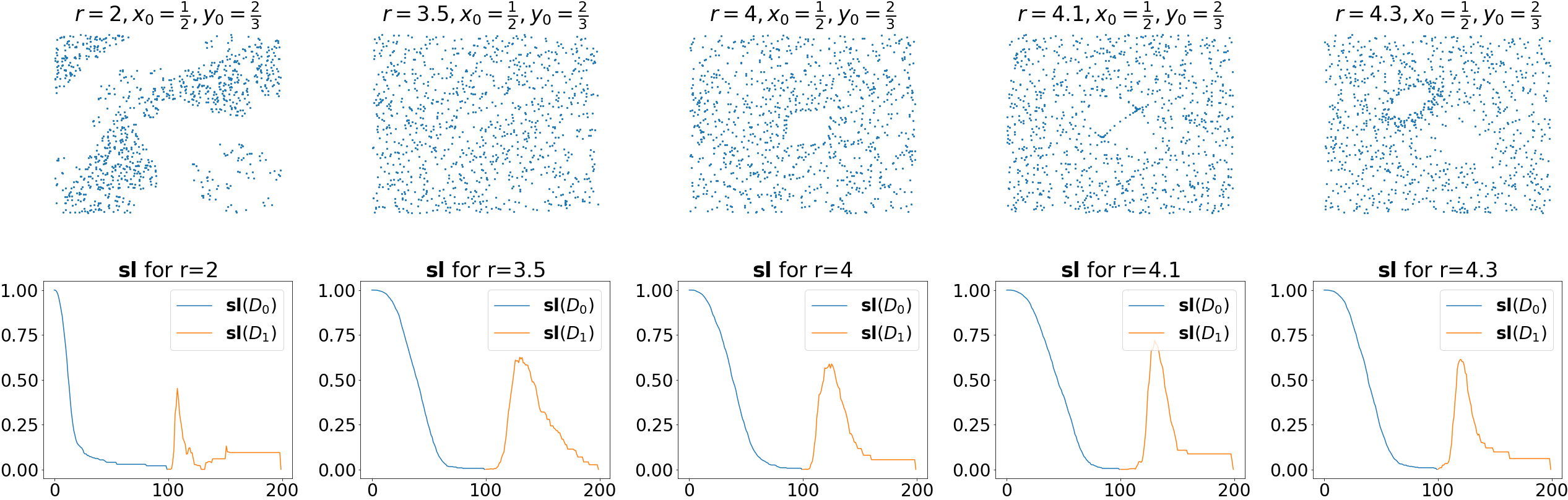
We are concerned with determining the parameter given a set of orbits. For this experiment, we generated 50 orbits for each parameter each with an initial position that is uniformly sampled from the unit square. We perform one 50/50 train/test split, then trained and scored each model using sci-kit learn’s [47] RandomForest algorithm with 100 estimators. We repeat the above process 100 times and the reported score for each model is the average of the 100 resulting scores.
Each observation in this dataset is a point cloud in . To compute the persistence diagrams for each point cloud, we use the Vietoris-Rips filtration via ripser[55]. Each of the models below use both 0 and 1-dimensional persistence diagrams, concatenating the resulting vectors for each. The infinite death value for 0-dimensional persistence was replaced with the max death value of the diagram. The models consisted of the following
- PC:
unaltered, normalized, and entropy versions of the Betti (), life (), and midlife () PCs each evaluated at 100 equally spaced points starting at the minimum birth value and ending at the maximum death value generating a 200 dimensional vector for each orbit and each model;
- :
the first three persistence landscapes each evaluated at 100 equally spaced points starting at the minimum birth value and ending at the maximum death value generating a 600 dimensional vector for each orbit;
- ECC:
the Euler Characteristic Curve each evaluated at 100 equally spaced points starting at the minimum birth value and ending at the maximum death value generating a 100 dimensional vector for each orbit;
- PIM:
Persistence Images with a resolution of and (the model proposed in [2]) flattened into a vector generating an 800-dimensional vector for each orbit;
- PS:
Persistence Statistics, which generate a 46 dimensional vector for each orbit. Given a diagram, the statistics are generated from the collections of lifespans and midlifes . On these collections, we calculate the mean, standard deviation, skewness, kurtosis, 10th, 25th, 50th, 75th, 90th percentiles, IQR, and coefficient of variation. Finally, we calculate the persistent entropy [3] of diagrams.
The reported scores appear in the last column of Table 3. The upper half of the table lists scores of the individual models described above, while the lower half list scores of the models above concatenated with persistence statistics. For this experiment, in both halves, we see that the PCs proposed in this paper, indicated by (PC) perform well.
In the upper half of the Table 3, we see performs the best. The life entropy curve (persistent entropy summary) [4] is the only model not originally proposed in this work to appear in the top 5. In the lower half of the table, we concatenated the original models with persistence statistics. This additional information seems to boost the classification power of the original models in most cases. With the addition of the persistence statistics, we see that the top 5 models are nearly equivalent.
6.2.2. Texture Classification
Texture classification is a classic task in the field of computer vision. In this paper, we apply our models to three texture databases.
- Outex0:
A database from the University of Oulu and consists of test suites each with a different challenge [46]. We focus on the test suites , which contains texture classes with grayscale images of each class that are by in size. The suite is equipped with preset 50/50 train/test splits. A score on the test suite is the average accuracy over all pre-defined splits.
- UIUCTex:
- KTH:
KTH’s Textures under varying Illumination, Pose and Scale (KTH-TIPS2b) is a database containing 81 200 by 200 grayscale images for each of its 10 textures [34]. As the name suggests, each texture class contains images of different scales, rotations, and illuminations. A score on this set is the average accuracy of 100 random 80/20 train/test splits.
The models use the same curves and methods as used in Section 6.2.1 with a few notable differences. Each observation for each database is an 8-bit grayscale image, which is a 2D array whose entries take integer values between 0 and 255. Persistence diagrams of an 8-bit image are calculated based on cubical complex and sublevel set filtration. Images have a guaranteed minimum birth of 0 and maximum death of 255. Moreover, all critical values are guaranteed to occur at integer values. Hence, for each diagram, all PC-based methods use the integers from to to generate a 256-dimensional vector. Moreover, as discussed in [20], computing persistence diagrams on images is affected by the boundary effect. Briefly, the boundary effect causes potential generators lying on the boundary of an image to go uncounted. To account for this, we also consider the persistent homology of the complement (or inverse) of an image. In total, each model considers four diagrams: the 0 and 1-dimensional diagrams for an image and its inverse. Figure 4 shows sample images from three texture database and their persistence curves. This leads to a 3072-dimensional vector for the first three landscapes model, 512-dimensional vector for the ECC method, a 92-dimensional vector for persistence statistics, a 1600-dimensional vector for persistence images, and 1024-dimensional vectors for all other PC-based methods. Finally, for persistence images, we set .
The first three columns of Table 3 displays our reported scores for the models on these three databases. In the upper half of the Table 3, we see that the normalized lifespan curve is among the top 5 performers on KTH-TIPS2b, coming in second behind persistence statistics and UIUCTex, coming in third. Persistence images performs well across all three texture datasets and performs best on UIUCTex. Perhaps most surprisingly is the performance of the standalone persistence statistics, which uses only 92-dimensional vectors to achieve the best score on both KTH-TIPS2b and Outex. Both the Euler Characteristic Curve and persistence landscapes fail to place here.
Remark 6.
It is interesting to compare the performance of persistence landscapes, which enjoy a high level of stability, with that of the Betti curve or persistent statistics, which do not. The numerical evidence here suggests that stability and classification performance might not be highly correlated.
In the lower half of the Table 3, we see again that persistence statistics improve the classification power of the original models. Top performers include normalized life, taking second and third on KTH-TIPS2b and UIUCTex respectively and persistence images, which was the top performer on KTH-TIPS2b and UIUCTex. Here, we see that the persistence landscapes model does not make it into the top 5, but the Euler Characteristic Curve model does on Outex and KTH-TIPS2b.
There are other TDA methods with applications to the same datasets. Outex0 has been studied through Sparse-TDA [33], persistence scale space kernel [49], metric learning for persistence diagrams [41], sliced Wasserstein Kernel [13], and persistence paths (specifically, the Betti kernel) [19]. The reported classification scores from those work are , , , , and respectively. In [48], authors applied their methods to both UIUCTex and KTH-TIPS2b, and their reported classification scores are , and , respectively. As a reference, the state-of-arts classification scores based on traditional bag of words based texture representation for these datasets are [30] for Outex0, [43] for UIUCTex, and [43] for KTH-TIPS2b.


| Outex0 | UIUCTex | KTH-TIPS2b | Orbits | |
| PS [20] | ||||
| s(PC) | ||||
| e(PC) | ||||
| (PC) | ||||
| (PC) | ||||
| [4] | ||||
| (PC) | ||||
| (PC) | ||||
| (PC) | ||||
| Land[8] | ||||
| ECC | ||||
| PIM[2] | ||||
| With PS | ||||
| +PS | ||||
| s+PS | ||||
| e+PS | ||||
| +PS | ||||
| +PS | ||||
| +PS | ||||
| +PS | ||||
| +PS | ||||
| +PS | ||||
| Land+PS | ||||
| ECC+PS | ||||
| PIM+PS |
6.3. Noise Handling
In order to demonstrate how each vectorization reacts to the noise, we design two experiments using the Outex0 and KTH-TIPS2b databases. We compare the performance of the normalized life curve, life entropy curve, first three landscapes, persistence statistics, and persistence images models by adding Gaussian noise to the testing set for the scoring process of each database. The noise was added with a standard deviation fixed at values in . The results are plotted in Figure 5(a)-(b). For Outex0, we see that persistence images are most resistant to noise and persistence statistics are least resistant. The normalized life, life entropy, and landscape curves perform similarly and begin to fall away from persistence images around . It seems in Figure 5(a) that these curves are leveling to a linear loss of score while the persistence image model seems to increase its loss over . In the KTH-TIPS2b experiment, we see a similar result as shown in Figure 5(b). Persistence images seem to be the most stable followed closely by normalized life and life entropy. Persistence statistics falls off quickly as do persistence landscapes. Because the images in KTH-TIPS2b are larger, the noise has less effect leading to more stability. This experiment demonstrates empirically how each vectorization reacts to noise under the random forest classification model. It would be interesting to investigate rigorously the relation between the performances of different classification models and stability of the vectorizations.
Finally we offer advice to practitioners that choose to use PCs. PCs carry interpretable information about the diagrams they are calculated from. In turn, the diagrams carry interpretable information about the topological properties of the underlying space. This allows domain experts to reasonably choose PCs to use in practice. However, the need for a learnable method is not far from our current setup. For example, take a general function as where . If is the sum statistic, then the resulting PC is one from which we can derive the life (, midlife (), and Betti () curves. We now have a class of PCs controlled by the parameters . Immediately, then, we may use a grid-search algorithm to select these parameters and learn the best curve for a given problem. We further note that both normalized and entropy-based curves are simple modifications of these basic curves, and hence fall under this grid-search framework as well. A deeper exploration into this facet of PCs will be left for future work.
6.4. Limitations and Considerations


As with any method, PCs come with some limitations. First and foremost, the information they carry about the original space is limited by the amount of information carried by the persistent homology. For example, the two images displayed in Figure 5(c)-(d) appear to have different patterns and yet they yield the same persistence diagrams. This leads to equal PCs and hence the images are indistinguishable via the normal persistence process. It can be useful to consider the original space in addition to the topology in the analysis, and model construction.
When working with PCs, or any vectorization method, one must also keep in mind the mesh (or resolution) of the vector. For image analysis, the choice of integer values from 0 to 255 is a natural one; however, in randomly generated point-cloud data, the choice is not so clear. The choice becomes less clear when dealing with a more dynamic dataset, such as one that does not have a minimum birth nor a maximum death value. Balancing the vector size, with the information retained is important to keep in mind. Finally, based on our experiments, we would recommend that one choose the normalized life curve among all other curves presented here for its stability, computational efficiency, and performance.
7. Generalization and Conclusion
PCs provide a simple general framework for generating functional summaries and vectorizations of persistence diagrams. These curves are compatible with machine learning algorithms, they can be stable. They are efficient to compute, and by choice of functions and statistics, one can alter the importance of points in different regions of the persistence diagrams. They also perform well in real applications as seen through the classification experiments for textures and the discrete dynamical system parameters. The theory and experimentation presented here are by no means complete. We conclude this paper by listing below several potential directions for further investigation.
Questions.
- Q1
In Theorem 1, the operator is fixed as . What conditions on the function or the statistic can lead to a more general and useful stability result?
- Q2
Several statistical properties, such as laws of large numbers, and stochastic convergence [16, 17, 9], of persistence landscapes has been established. Since persistence landscapes fall under the PC framework, it would be interesting to investigate general conditions on and so that the same properties hold.
- Q3
The Euler Characteristic Transform [56] was proved to be a sufficient statistic for distributions on the space of subsets of that can be written as simplicial complexes where , and was applied to shape analysis. It would be interesting to generalize this concept to PCs.
- Q4
Is there a statistical framework to perform “curve selection” that will produce an optimal or near optimal set of curves for modeling?
- Q5
Since Lemma 1 can be generalized to the -norm, it would be interesting to investigate the stability results with respect to distance.
References
- [1] PersistenceImages. https://gitlab.com/csu-tda/PersistenceImages, 2019.
- [2] H. Adams, T. Emerson, M. Kirby, R. Neville, C. Peterson, P. Shipman, S. Chepushtanova, E. Hanson, F. Motta, and L. Ziegelmeier, Persistence images: A stable vector representation of persistent homology, The Journal of Machine Learning Research, 18 (2017), pp. 218–252.
- [3] N. Atienza, R. Gonzalez-Diaz, and M. Soriano-Trigueros, A new entropy based summary function for topological data analysis, Electronic Notes in Discrete Mathematics, 68 (2018), pp. 113 – 118. Discrete Mathematics Days 2018.
- [4] N. Atienza, R. González-Díaz, and M. Soriano-Trigueros, On the stability of persistent entropy and new summary functions for TDA, CoRR, abs/1803.08304 (2018).
- [5] G. Bell, A. Lawson, C. N. Pritchard, and D. Yasaki, The space of persistence diagrams fails to have yu’s property a, 2019.
- [6] P. Bendich, J. S. Marron, E. Miller, A. Pieloch, and S. Skwerer, Persistent homology analysis of brain artery trees, The annals of applied statistics, 10 (2016), p. 198.
- [7] E. Berry, Y.-C. Chen, J. Cisewski-Kehe, and B. T. Fasy, Functional summaries of persistence diagrams, Journal of Applied and Computational Topology, 4 (2020), pp. 211–262.
- [8] P. Bubenik, Statistical topological data analysis using persistence landscapes, The Journal of Machine Learning Research, 16 (2015), pp. 77–102.
- [9] , The persistence landscape and some of its properties, Abel Symposia, (2020), p. 97–117.
- [10] P. Bubenik and T. Vergili, Topological spaces of persistence modules and their properties, Journal of Applied and Computational Topology, 2 (2018), p. 233–269.
- [11] P. Bubenik and A. Wagner, Embeddings of persistence diagrams into hilbert spaces, 2019.
- [12] M. Carrière and U. Bauer, On the metric distortion of embedding persistence diagrams into separable hilbert spaces, in Symposium on Computational Geometry, 2019.
- [13] M. Carrière, M. Cuturi, and S. Oudot, Sliced Wasserstein kernel for persistence diagrams, in Proceedings of the 34th International Conference on Machine Learning, D. Precup and Y. W. Teh, eds., vol. 70 of Proceedings of Machine Learning Research, International Convention Centre, Sydney, Australia, 06–11 Aug 2017, PMLR, pp. 664–673.
- [14] M. Carrière, F. Chazal, Y. Ike, T. Lacombe, M. Royer, and Y. Umeda, Perslay: A neural network layer for persistence diagrams and new graph topological signatures, 2019.
- [15] C. J. Carstens and K. J. Horadam, Persistent homology of collaboration networks, Mathematical problems in engineering, 2013 (2013).
- [16] F. Chazal, B. Fasy, F. Lecci, B. Michel, A. Rinaldo, and L. Wasserman, Subsampling methods for persistent homology, in International Conference on Machine Learning, 2015, pp. 2143–2151.
- [17] F. Chazal, B. T. Fasy, F. Lecci, A. Rinaldo, and L. Wasserman, Stochastic convergence of persistence landscapes and silhouettes, in Proceedings of the thirtieth annual symposium on Computational geometry, ACM, 2014, p. 474.
- [18] Y.-C. Chen, D. Wang, A. Rinaldo, and L. Wasserman, Statistical analysis of persistence intensity functions, arXiv preprint arXiv:1510.02502, (2015).
- [19] I. Chevyrev, V. Nanda, and H. Oberhauser, Persistence paths and signature features in topological data analysis, IEEE Transactions on Pattern Analysis and Machine Intelligence, 42 (2020), pp. 192–202.
- [20] Y.-M. Chung and S. Day, Topological fidelity and image thresholding: A persistent homology approach, Journal of Mathematical Imaging and Vision, (2018), pp. 1–13.
- [21] Y.-M. Chung, C.-S. Hu, A. Lawson, and C. Smyth, Topological approaches to skin disease image analysis, in 2018 IEEE International Conference on Big Data (Big Data), IEEE, 2018, pp. 100–105.
- [22] D. Cohen-Steiner, H. Edelsbrunner, and J. Harer, Stability of persistence diagrams, Discrete & Computational Geometry, 37 (2007), pp. 103–120.
- [23] D. Cohen-Steiner, H. Edelsbrunner, J. Harer, and Y. Mileyko, Lipschitz functions have l p-stable persistence, Foundations of computational mathematics, 10 (2010), pp. 127–139.
- [24] V. De Silva, R. Ghrist, et al., Coverage in sensor networks via persistent homology, Algebraic & Geometric Topology, 7 (2007), pp. 339–358.
- [25] V. Divol and T. Lacombe, Understanding the topology and the geometry of the space of persistence diagrams via optimal partial transport, Journal of Applied and Computational Topology, (2020), pp. 1–53.
- [26] P. Dlotko, Persistence representations, in GUDHI User and Reference Manual, GUDHI Editorial Board, 3.1.1 ed., 2020.
- [27] I. Donato, M. Gori, M. Pettini, G. Petri, S. De Nigris, R. Franzosi, and F. Vaccarino, Persistent homology analysis of phase transitions, Physical Review E, 93 (2016), p. 052138.
- [28] H. Edelsbrunner and J. Harer, Computational Topology: An Introduction, Miscellaneous Books, American Mathematical Society, 2010.
- [29] H. Edelsbrunner, D. Letscher, and A. Zomorodian, Topological persistence and simplification, in Proceedings 41st Annual Symposium on Foundations of Computer Science, IEEE, 2000, pp. 454–463.
- [30] H. G. Feichtinger and T. Strohmer, Gabor analysis and algorithms: Theory and applications, Springer Science & Business Media, 2012.
- [31] M. Ferri, P. Frosini, A. Lovato, and C. Zambelli, Point selection: A new comparison scheme for size functions (with an application to monogram recognition), in Asian Conference on Computer Vision, Springer, 1998, pp. 329–337.
- [32] P. Frosini, Measuring shapes by size functions, in Intelligent Robots and Computer Vision X: Algorithms and Techniques, vol. 1607, International Society for Optics and Photonics, 1992, pp. 122–134.
- [33] W. Guo, K. Manohar, S. L. Brunton, and A. G. Banerjee, Sparse-tda: Sparse realization of topological data analysis for multi-way classification, IEEE Transactions on Knowledge and Data Engineering, 30 (2018), pp. 1403–1408.
- [34] E. Hayman, B. Caputo, M. Fritz, and J.-O. Eklundh, On the significance of real-world conditions for material classification, in European conference on computer vision, Springer, 2004, pp. 253–266.
- [35] J. Hein, Discrete Mathematics, Discrete Mathematics and Logic Series, Jones and Bartlett Publishers, 2003.
- [36] T. Kaczynski, K. Mischaikow, and M. Mrozek, Computational Homology, Applied Mathematical Sciences, Springer New York, 2004.
- [37] G. Kusano, Y. Hiraoka, and K. Fukumizu, Persistence weighted gaussian kernel for topological data analysis, in International Conference on Machine Learning, 2016, pp. 2004–2013.
- [38] A. Lawson, PersistenceCurves (a python package for computing persistence curves). https://github.com/azlawson/PersistenceCurves, 2018.
- [39] A. Lawson, On the Preservation of Coarse Properties over Products and on Persistence Curves, PhD thesis, The University of North Carolina at Greensboro, 2019.
- [40] S. Lazebnik, C. Schmid, and J. Ponce, A sparse texture representation using local affine regions, IEEE Transactions on Pattern Analysis and Machine Intelligence, 27 (2005), pp. 1265–1278.
- [41] C. Li, M. Ovsjanikov, and F. Chazal, Persistence-based structural recognition, in Proceedings of the IEEE Conference on Computer Vision and Pattern Recognition, 2014, pp. 1995–2002.
- [42] L. Li, W.-Y. Cheng, B. S. Glicksberg, O. Gottesman, R. Tamler, R. Chen, E. P. Bottinger, and J. T. Dudley, Identification of type 2 diabetes subgroups through topological analysis of patient similarity, Science translational medicine, 7 (2015), pp. 311ra174–311ra174.
- [43] L. Liu, J. Chen, P. Fieguth, G. Zhao, R. Chellappa, and M. Pietikäinen, From bow to cnn: Two decades of texture representation for texture classification, International Journal of Computer Vision, 127 (2019), pp. 74–109.
- [44] Y. Mileyko, S. Mukherjee, and J. Harer, Probability measures on the space of persistence diagrams, Inverse Problems, 27 (2011), p. 124007.
- [45] T. Nakamura, Y. Hiraoka, A. Hirata, E. G. Escolar, and Y. Nishiura, Persistent homology and many-body atomic structure for medium-range order in the glass, Nanotechnology, 26 (2015), p. 304001.
- [46] T. Ojala, T. Maenpaa, M. Pietikainen, J. Viertola, J. Kyllonen, and S. Huovinen, Outex-new framework for empirical evaluation of texture analysis algorithms, in Object recognition supported by user interaction for service robots, vol. 1, IEEE, 2002, pp. 701–706.
- [47] F. Pedregosa, G. Varoquaux, A. Gramfort, V. Michel, B. Thirion, O. Grisel, M. Blondel, P. Prettenhofer, R. Weiss, V. Dubourg, J. Vanderplas, A. Passos, D. Cournapeau, M. Brucher, M. Perrot, and E. Duchesnay, Scikit-learn: Machine learning in Python, Journal of Machine Learning Research, 12 (2011), pp. 2825–2830.
- [48] J. A. Perea and G. Carlsson, A klein-bottle-based dictionary for texture representation, International Journal of Computer Vision, 107 (2014), pp. 75–97.
- [49] J. Reininghaus, S. Huber, U. Bauer, and R. Kwitt, A stable multi-scale kernel for topological machine learning, in Proceedings of the IEEE conference on computer vision and pattern recognition, 2015, pp. 4741–4748.
- [50] E. Richardson and M. Werman, Efficient classification using the Euler characteristic, Pattern Recognition Letters, 49 (2014), pp. 99–106.
- [51] B. Rieck, F. Sadlo, and H. Leitte, Topological machine learning with persistence indicator functions, in Topological Methods in Data Analysis and Visualization, Springer, 2017, pp. 87–101.
- [52] J. Rotman, An Introduction to Algebraic Topology, Graduate Texts in Mathematics, Springer New York, 1998.
- [53] M. Saadatfar, H. Takeuchi, V. Robins, N. Francois, and Y. Hiraoka, Pore configuration landscape of granular crystallization, Nature communications, 8 (2017), p. 15082.
- [54] G. Tauzin, U. Lupo, L. Tunstall, J. B. Pérez, M. Caorsi, A. Medina-Mardones, A. Dassatti, and K. Hess, giotto-tda: A topological data analysis toolkit for machine learning and data exploration, 2020.
- [55] C. Tralie, N. Saul, and R. Bar-On, Ripser.py: A lean persistent homology library for python, The Journal of Open Source Software, 3 (2018), p. 925.
- [56] K. Turner, S. Mukherjee, and D. M. Boyer, Persistent homology transform for modeling shapes and surfaces, Information and Inference: A Journal of the IMA, 3 (2014), pp. 310–344.
- [57] K. Turner and G. Spreemann, Same but different: Distance correlations between topological summaries, 2019.
- [58] Y. Umeda, Time series classification via topological data analysis, Information and Media Technologies, 12 (2017), pp. 228–239.
- [59] A. Zomorodian and G. Carlsson, Computing persistent homology, Discrete & Computational Geometry, 33 (2005), pp. 249–274.
Appendix A Explicit Calculations of Bounds Using Theorem 1
In this section, we will assume and utilize the definitions of the curves defined in Table 1. To ease notation we will write in place of and analogously for . We recall the following definitions.
| (31) | ||||
| (32) | ||||
| (33) | ||||
| (34) |
A.1. Betti-based Curves
In this section we consider the curves based on the Betti number. As we will see the function for each of the curves in this section is not continuous at the diagonal, which causes the bounds to be large.
A.1.1. Betti Number Curve ()
Recall that the Betti curve is by taking when , and 0 otherwise. The values for and are straightforward to calculate.
On the other hand, notice that if then we have when and 0 otherwise. This means that the worst case scenario for the Betti curve is when all points are paired with the diagonal yielding the following values
Hence, we may conclude by Theorem 1 that
| (35) | ||||
| (36) |
Neither of these bounds are desirable. Not only as the number of points increase both bounds tend to infinity, but also both bounds contain constants that are irrelevant to nor . Moreover, the same occurs as the minimum lifespan grows.
A.1.2. Normalized Betti Curve ()
According to Definition 2, we may define the normalized Betti curve by taking when , and otherwise. Again we can get the values quickly
On the other hand, for all
Hence, we may conclude by Theorem 1 that
| (37) | ||||
| (38) |
Even with the normalization, these two bounds still depend heavily on the number of diagram points and the maximum lifespan.
A.1.3. Betti Entropy Curve ()
By Definition 3, the Betti Entropy Curve is defined by taking when and 0 otherwise. If the points of and are indexed according to the optimal matching for distance and if (so that ), then by Lemma 3
A.2. Midlife-based Curves
For this section, we will assume that all birth and death values are non-negative (so that ). The midlife-based curves, similar to the lifespan based curves, benefit from continuous functions. Moreover, the bounds in this section take a form similar to those of the lifespan-based counterparts. For this section, we will use the notation , , and . Finally, because we are assuming non-negativity, we also have .
A.2.1. Midlife Curve
The midlife curve take . The values and . We see then that for any
If instead the indexing follows the optimal matching for we see
Therefore by Theorem 1 we conclude
| (41) | ||||
| (42) |
A.2.2. Normalized Midlife Curve
The normalized midlife curve take
. The values and . Moreover, suppose . We note that .
Moreover,
Therefore by Theorem 1 we conclude
| (43) | ||||
| (44) |
A.2.3. Midlife Entropy Curve
In this final section we will discuss the bounds for the midlife entropy curve, which uses . Straightforward calculation reveals and . The bounds recovered for midlife entropy are the same as for life entropy. That is, if , Theorem 1 guarantees that
| (45) | ||||
| (46) |
Appendix B Proof of Lemma 4 in Section 5.4
For convenience, we will restate the lemma here:
Lemma.
Let , where for . Then
Proof.
We need similar estimates to that in Lemma 1. Consider
where for . Recall that can also be expressed as
Finally, define .
Case 1: and . Then
| (47) |
Thus, .
Case 2: and . Then we have three maximums to consider.
| (48) |
For the first, there are two subcases: and . In either case we see
| (49) |
Observe that for , we have . In each of the cases above, . Thus, . Similarly, one may verify that when , .
When , there are 5 sub cases to consider.
- i)
;
- ii)
;
- iii)
;
- iv)
;
- v)
.
One may verify that each case is bounded by .
Case 3: . We have three maximums to consider.
| (50) |
The first and third maximums follow the same arguments as in case 2. For the middle maximum, we see that we have four subcases
- i)
;
- ii)
;
- iii)
;
- iv)
.
For i), note that thus, . We complete this case by noting that for all , . Moreover is decreasing over the interval . Therefore, the difference is maximized at and the difference is precisely .
One may verify the remaining cases satisfy the conclusion. ∎